a comprehensive approach to the 3d geological modelling of ... · a comprehensive approach to the...

Estonian Journal of Earth Sciences, 2015, 64, 2, 173–188 doi: 10.3176/earth.2015.25

173

A comprehensive approach to the 3D geological modelling of sedimentary basins: example of Latvia, the central part of the Baltic Basin

Konrāds Popovs, Tomas Saks and Jānis Jātnieks

Faculty of Geography and Earth Sciences, University of Latvia, 19 Raina Blvd., LV 1580 Riga, Latvia; [email protected] Received 12 June 2014, accepted 24 October 2014 Abstract. This paper presents a semi-automatic approach adapted to the modelling of the geological structure of sedimentary basins. The modelling approach is based on developing the algorithm of the main geological processes so that the geometrical relationship is automatically defined between model elements. The algorithm is based on the assumption that sedimentary basins are formed as a result of the repeated sequence of sedimentation, faulting and erosion. This approach allows of successful modelling of the geological structure of the sedimentary basins with limited data coverage: stratigraphic intervals from well logs describing the thicknesses of sedimentary strata and a limited amount of structural data. Sedimentary layers are handled by modelling assuming non-eroded thickness distribution and using geometrical adjustment from the known fault displacements. As a result geometrical relationships of the model layers are deduced automatically in the presence of unconformities.

An application of this methodology, a 3D geological model of Latvia, the central part of the Baltic Basin, is presented. The results show that this model is geologically reasonable for achieving the structural and stratigraphic concepts. Key words: 3D geology, geometrical modelling, geological rules, thickness constraints, sedimentary basins, Latvia.

INTRODUCTION Geological maps and interpreted cross sections have long been the basic source in solving geological issues and the most frequent way of representing the geological setting. Nowadays the usefulness of 3D geometrical models has been recognized for better understanding of the geological setting, reducing the uncertainties in many geological fields (Houlding 1994; Wu et al. 2005). Correct understanding of the stratigraphy and origin of geological structures using 3D methods unfolds some limitations of the 2D approaches (Bardossy & Fodor 2001; Bistacchi et al. 2008; Caumon et al. 2009).

It is assumed that the 3D geological models require high-density data. When constructing the geological structure manually, it is hard to deal with geological uncertainties using scarce or sparsely distributed data (Kauffman & Martin 2008; Carrera et al. 2009; Caumon et al. 2009). When it comes to basin-scale interpretations, e.g., the thickness distribution of the sequence, often the available data are too general to minimize the uncertainty related to the geological structure. Although specialized software allows modelling complex large-scale geological bodies, building a 3D model is still a challenge. A geological map contains the interpretation of survey

data and the level of knowledge at the time of its creation and often does not enclose correct topological relations between geological objects where multiple maps are stacked together, especially in older maps. Geophysical data, such as deep seismic, gravity or magnetics, are more favourable. However, on a regional scale often such data are not available or are limited. Thereby, to improve the quality of the geological models, algorithmization of the geological history is needed.

A comprehensive mechanism to handle prerequisites of the sedimentary sequence is lacking. Thus it is difficult to construct the geometrical relationships between complicated sedimentary strata utilizing the existing modelling methods, which require extensive manual interaction.

In this paper we outline the geological modelling approach for the construction of the geometry of sedi-mentary basins. The approach is based on the extension in 3D of the simple assumption by Dahlstrom (1969) that post-depositional deformations produce no significant change in the sedimentary strata volume where the thickness and length of the strata in a cross-sectional plane remain unchanged, except as a result of erosion. Assuming that the tectonic deformation occurs in sequential cycles where subsequent tectonic stages are

Estonian Journal of Earth Sciences, 2015, 64, 2, 173–188

174

separated by a regional unconformity, we model sedi-mentary layer thicknesses and reconstruct main erosional surfaces based on Dahlstrom’s (1969) assumption. The procedure is maintained using borehole data and a structural dataset describing fault location and displace-ment for only one geological surface of each tectonic sequence. The geological history is integrated into the modelling procedure so that the basic geometrical relation-ship between model layers are automatically defined.

The proposed method has been implemented within the MOSYS modelling system (Virbulis et al. 2012) as a unique modelling algorithm. As an application, the 3D geological model of Latvia was created.

Certain geological modelling has previously been done in the neighbouring areas (Lazauskienė & Šliaupa 2002; Vallner 2003) and regional studies including the 3D characterization of the geological structure (Poprowa et al. 1999; Lazauskienė et al. 2002; Šliaupa 2002; Shogenova et al. 2009; Spalvins et al. 2012; Virbulis et al. 2012, 2013) have been carried out in Latvia. Nevertheless, direct modelling of the 3D geometry of the geological structure of Latvia has not been performed so far.

The past studies have provided substantial geo-logical information, including an extensive borehole database (Takcidi 1999), as well as a set of structural (Brangulis & Kaņevs 2002) and geological maps (Brangulis et al. 2000). However, structural data describing the tectonics is the most important factor that determines the geometry of the basin structure. Unfortunately it is available only for four geological surfaces as a set of structural maps. The premise of this study is that 3D modelling using the proposed approach can reveal more detailed information than the 2D approach in previous interpretations and is applicable to the geometrical modelling of sedimentary basins. METHODOLOGY

Modelling approach The dominant geometrical shape of a sedimentary basin is sequential, regular stacking of sedimentary strata and their interfaces complicated by faults and intersections of strata due to various geological processes. Strata can be classified as ‘complete’ or ‘missing’ in terms of their integrity and spatial distribution, e.g., one that is distributed continuously in a given area, or discontinuously, inter-secting with other strata (Turner 2006; Zhu et al. 2012). On a regional scale it is substantial to define and simulate these conditions automatically.

The modelling approach proposed herein is based on the extension in 3D of the simple assumption proposed

by Dahlstrom (1969). According to this assumption, on a regional scale post-depositional deformation produces no significant change in the volume of sedimentary strata, e.g., strata thickness in a cross-sectional plane remained unchanged except as a result of erosion. We assume that present sedimentary basins were formed as a result of a repeated sequence of geological events – sedimentation, faulting and erosion. Therefore, instead of focusing on each stratum separately, we systematize the geological column within the tectonic sequence with similar geological regularities.

Assuming that the tectonic deformation occurs in sequential cycles and each subsequent tectonic stage stratum is separated by a regional unconformity, we algorithmize these assumptions. This is done by recon-structing the thicknesses of original layers before erosion and after that by slicing them along known fault lines and applying known fault displacements to all the layers within each tectonic stage. Therefore an applicable layer thickness is adjustable by taking the amount of erosion by the presence of regional unconformities into account.

This approach can be applied if borehole data describing the thickness variations of each modelled layer and the structural dataset with known fault displace-ments (further in text – base surfaces) at least for one geological surface inside each tectonic sequence is available.

To meet the prerequisites of a geological structure, the model framework is based on a clear well-organized depositional sequence dividing sedimentary strata by adherence to tectonic sequences. The model is formed of regional erosion interfaces with distinguished vertical traceability of faults in the geological column by stacking the available base surfaces and reconstructing erosion interfaces. Erosion surfaces must be considered when superimposing the thickness of the overlying layer – if the overlying layer is faulted, the same displacement must be reflected in the erosion surface (Fig. 1A).

The geometry of sedimentary layers within each tectonic sequence is based on borehole data describing the non-eroded thickness of each layer. The applicable layer topography is obtained by sequentially filling the empty volume between the base and erosion surfaces with modelled slices. As a result, known fault displace-ments are transferred from base surfaces to the affected layer sequence where the resultant topography of all sedimentary layers is logically coherent between them (Fig. 1B). When the full thickness of a particular layer is unknown, but consecution can be identified (4th layer in Fig. 1C), we can presume that the layer is topo-graphically similar to the underlying layer. Therefore, the layer volume can be obtained by filling the empty space between the underlying layer and unconformity.

K. Popovs et al.: 3D modelling of sedimentary basins

175

Fig. 1. Schematic drawing of principles for the proposed modelling approach. A, construction of the model framework; B, construction of sedimentary layers with known full thickness; C, construction of sedimentary layers with unknown full thickness. BH 1–BH 3, boreholes with layer boundaries; 1–5, geological layers; vertical lines – faults; dashed lines – base surfaces; dotted line – erosion surface. Modelling workflow The proposed modelling approach was integrated within the MOSYS modelling system (Virbulis et al. 2012) as algorithmized workflow. MOSYS is a Python language script-based package suitable for the generation of geometrical models of a geological structure. The usage of MOSYS is abstracted in the system of logical pre-defined operations and user-defined command systems (algorithms) managed through the scripting and command line interface. The system provides compulsory documen-tation of all parameter settings and repeatable creation of the geological structure. The developed workflow has a high level of the automation process and strong adaptability.

Model geometry is constructed layer-wise on a 2D unstructured triangular mesh where each layer is represented as a volumetric element. The triangular mesh incorporates characteristic features such as fault lines and borehole points as mesh nodes. Mesh details are

variable, with a possibility of freely defining the average size of the triangles and refine step. Known faults were scripted as dissecting lines where the 2D mesh was cut along them, duplicating the mesh nodes along the lines. Borehole locations in the mesh structure were incorporated as single points. The areas between the lines and points were triangulated with the resulting length of the triangle edges of 1–4 km.

Data interpolation was done by linear interpolation. Extrapolation was handled by extrapolating the average value trend within the data set to the area where values were not defined (Virbulis et al. 2012).

Three main steps are followed in the workflow. First, according to the available information, a clear and well-organized depositional sequence of all stratigraphic units, fault traceability and erosion events are obtained. By the division of the depositional sequence by adherence to tectonic sequences a model framework is created (Fig. 1A), which defines major erosional interfaces and systematizes vertical traceability of known faults according to the stratigraphic sequence. This allows the definition of fault displacements and sets limits to the distribution of the sedimentary layers.

The next step comprises the modelling of depositional layers (Fig. 1B). It is necessary to use the extrapolation method to maintain regional thickness distribution to the model domain by interpolating the thickness distribution of sedimentary layers before erosion. For this purpose a sequential algorithm is developed for all layers containing linear interpolation and extrapolation of non-eroded thickness point type data from borehole columns.

At the final step the empty volume between base surfaces and erosion surfaces is filled sequentially. The layer topography and fault displacements of each layer are transferred within each tectonic sequence following the stratigraphy and structural concepts of the geological column. For layers that lie directly below erosion surfaces with extents wedged into it, non-eroded thickness data are not available. Such layers are constructed volumetri-cally by filling the empty space between the underlying layer and the erosion surface (Fig. 1C).

As a result, topological relations of all model layers are controlled automatically by relationships between sedimentary layers and erosion interfaces – modelled topography of subjacent layers is wedged out in intersects with erosion surfaces or terminated along fault lines. GEOLOGICAL MODEL OF LATVIA

Geological setting The study area is a part of the East European Platform and covers the central part of the Baltic Basin (Fig. 2). The sedimentary cover is up to 2 km thick and consists of


176

Fig. 2. The southeastern Baltic region and structure map of the Baltic Basin (modified after Šliaupa & Hoth 2011). The contour lines indicate the depth of the top of the Precambrian crystalline basement. The dotted lines show major fault zones. Dark grey marks the research area.

Ediacaran, Palaeozoic, Mesozoic and Cenozoic deposits (Lukševičs et al. 2012). The layering of the sedimentary cover is subhorizontal, however, during several tectonic cycles the geological setting has been complicated by various tectonic structures (Fig. 3).

The Ediacaran and lower Cambrian Lontova Formation belongs to the Ediacaran sequence which discordantly overlies the Precambrian basement. Ediacaran rocks are distributed in the eastern part of Latvia as well as in a small area in western Kurzeme. The thickness of these rocks is about 50–300 m in eastern Latvia and under 50 m in Kurzeme (Lukševičs et al. 2012).

Cambrian, Ordovician and Silurian deposits constitute the Caledonian sequence. The surface elevation of this sequence generally follows the structure of the crystalline basement (Brangulis & Kaņevs 2002). This sequence is faulted and its geometry is mainly controlled by the amount of displacement along the faults and rate of erosion during the Late Silurian–Early Devonian. The faulting occurred predominantly via a number of reactivated normal faults in the crystalline basement at the end of the Silurian. As a result this sequence was faulted into numerous tectonic blocks and unequally eroded (Lukševičs et al. 2012).

Fig. 3. Geological and structural characterization of Latvia (modified after Brangulis & Kaņevs 2002). A, simplified geologicalmap of the Caledonian structural complex; B, simplified geological map of the Hercynian structural complex; C, simplifiedgeological cross section. Thick lines denote major faults. The dotted area in A shows the lower Devonian Gargzdu series; locationof the cross section is indicated by a dashed line in B. AR–PR, Precambrian crystalline basement; Cm–V, Cambrian–Ediacaransequence; O1–3, Ordovician sequence; Sln, Silurian, Llandovery; Sw, Silurian, Wenlock; Sld, Silurian, Ludlow; Spr, Silurian, Pridoli;D1, Lower Devonian; D2, Middle Devonian; D3, Upper Devonian; C1, Carboniferous; P2–T1, Permian–Triassic sequence; Q, Quaternary.


177

The Cambrian is predominantly composed of 50–300 m thick marine sandstones, siltstones and clays. The Ordovician and Silurian sequences are represented by deeper marine facies – marine clays, limestone and marls. The thickness of the Ordovician varies from 50–100 m in the northern part to 200–250 m in the central and eastern parts of the Baltic Basin. The thickness of Silurian sediments varies from 15 m in the eastern part to 650 m in the western part of the basin (Gailite et al. 1987). Regional thickness variation of the Ordovician and Cambrian sediments is controlled by the topography of the crystalline basement, and the surface charac-teristics of these layers are similar. Contrary to earlier suggestions that some faults display reversed displace-ments (Brangulis & Kaņevs 2002), the newest analyses suggest that all of the known faults of the Caledonian stage are reactivated normal faults of the crystalline basement (Ukass et al. 2012).

The following Hercynian stage sequence, which lasted from the Devonian to the Carboniferous, is up to 1000 m thick (Brangulis & Kaņevs 2002). The average thickness of this geological sequence is approximately 400 m in eastern and up to 600–1000 m in SW Latvia. This sequence discordantly covers the Caledonian sequence in the whole of Latvia. It consists mainly of sandstones and limestones formed predominantly under shallow marine conditions (Lukševičs et al. 2012).

Sediments of this stage are less deformed with less pronounced fault activity. Some hints of the basin inversion tectonics can be traced during the Narva Stage

(Ukass et al. 2012), which is supported by the sedimentary record of the Narva Stage (Tänavsuu-Milkeviciene et al. 2009). Later deformation stages can be traced in the very southwest corner of Latvia, where some normal displacement along the Liepaja–Saldus fault of probably Carboniferous age is recorded (Brangulis & Kaņevs 2002).

Carboniferous, Permian, Triassic and Jurassic sedi-ments are found only in small areas in SW Latvia, while the Cretaceous, Palaeogene and Neogene are absent. Quaternary deposits discordantly cover the Middle Devonian to Jurassic. The structure of the Quaternary sequence is very complicated due to a large amount of small-scale glaciotectonic structures and high hetero-geneity of deposits and are not discussed in this study. Source data and processing The data used in this study are diverse by their type, resolution, heterogeneity and density. Thereby, data sources were classified according to priority, depending on the type and the purpose of their application (Table 1).

Stratigraphic intervals from well logs are summarized in the database developed by the Latvian Environment, Geology and Meteorology Agency (LEGMA). The data corresponding to the topography and thickness of geo-logical layers were used from this database. Topography data and fault location with corresponding displace-ments were taken from available structural geology maps. The data set was supplemented by distribution

Table 1. Geological data sources, type and usage priority after resolution and purpose in model development

Type Information Resolution Priority Purpose Source

Bor

ehol

es Layer thickness

and topography data

Vertical resolution 0.5 m

1 Interpretation of layer thicknesses and topography, control of results

LEGMA Borehole database, 26 155 boreholes (Takcidi 1999)

1 Construction of fault structures

Str

uctu

ral m

aps

Location of fault lines, slip amplitude along faults, relief data

M 1 : 500 000; Isoline steps: 100,

25, 10 m 2 Interpretation of layer

topography

Surfaces of the crystalline basement, Ordovician, middle Devonian Pärnu Stage, upper Devonian Amata Stage (Brangulis & Kaņevs 2002)

M 1 : 200 000 Geological map of the Sub-Quaternary surface (Brangulis et al. 2000) C

arto

grap

hic

data

Geo

logi

cal m

aps

Extents of geological layers

M 1 : 500 000

3 Construction of layer borders

Geological map of the Caledonian structural complex (Brangulis et al. 2000)


178

polygons of geological layers from the geological map of the Sub-Quaternary surface and Caledonian structural complex. The digital relief model CIGAR SRTM V4.1 (Jarvis et al. 2008) was used as topographical surface.

Borehole logs were utilized for modelling with the highest priority. Structural maps used for modelling rely on the interpretation of the seismic and borehole data at the time of their compilation and this information is considered to be a general summary of seismic data of the research area. Fault locations and displacements summarized in structural maps with supplementation of borehole data were defined as a main data source for the modelling of the faults. Large-scale topography data from these maps were used as a supplementary data set for these surfaces. These geological surfaces are referred to as ‘base surfaces’. Tertiary priority was assigned to geological maps of the Sub-Quaternary surface and the Caledonian structural complex. Although detailed maps have been produced on 1 : 200 000 and 1 : 500 000 scales (Brangulis et al. 2000), they contain considerable offset against the boreholes as they do not comprise all available borehole data.

All data were normalized to the BalticTM93 coordinate system. Borehole data were organized in the MySQL database and cartographic data stored in attributed ESRI shapefiles providing direct integration within MOSYS (Virbulis et al. 2012).

For the map digitization and processing in the GIS environment, 2D topology rules were applied to ensure the geometric consistency of digitized objects. For example, they do not permit intersections of the vectorized lines, overlapping of digitized polygons and perform the merging of multipart objects as defined by Kauffman & Martin (2008).

Fault displacements from structural maps were converted to point data in several steps for further implementation in the modelling procedure. The interpolation of vectorized contours along with layer topography surface data from boreholes was applied using the Spline with Barriers interpolation toolbox in ArcGIS 9.3 (Zoraster 2003), where fault lines from structural maps served as barriers for the surface interpolation. As a result a 50 m cell raster was created. Next, a point vector file was generated with a 50 m tolerance on both sides of the fault lines and elevation values from the raster meshes were assigned for each surface. This point set served as an input for the reconstruction of the displacements along known faults for base surfaces.

The geological layers in borehole logs were divided following the Latvian stratigraphic chart (Stinkulis 2003). Records corresponding to each geological index were separated into two groups: (1) records of full layer thickness and (2) records of partial layer thickness where

only the upper boundary of the layer is described. The latter, together with indirect indexes, were used only to construct base surfaces. Model conceptualization and building The depositional sequence was generalized based on borehole data where model layers were distinguished at as detailed stratigraphic level as possible after Stinkulis (2003). The layers were divided into the following sequences considering tectonic cycles and major erosion events: the Caledonian sequence Cm–D1gr, the Hercynian sequence D1km–C, the Alpine sequence P–J and a separate Quaternary layer. The layers corresponding to the Ediacaran were treated within the Cambrian sequence. The Precambrian crystalline basement was defined as the lowermost model boundary (Fig. 4).

As suggested by Brangulis & Kaņevs (2002), the fault displacements within the study area are considered as vertically constant, allowing the use of the displace-ment data from the crystalline basement and Ordovician base surfaces to model fault structures in the Caledonian stage, Middle Devonian Pärnu and Upper Devonian Amata Base surfaces to the Hercynian stage. Since fault displacements in Permian–Jurassic sediments are within a few tens of metres within the study area, these are not included in this paper.

In this research we focused on the most important erosion events – the erosion event between the late Silurian and early Devonian (Šliaupa 2002), expressed as significant erosion of the Silurian and partly Ordovician deposits, and a large glacial erosion event during the Cenozoic (Marrota & Sabadini 2004), expressed as the erosion of deposits of the Lower Devonian Gargzdu Formation to the Jurassic sequence. The erosion event in the early Permian is neglected in this research since it does not have a decisive role on layer geometry in the study area.

The model framework was constructed from four base surfaces and two erosion surfaces (Fig. 4). The base surfaces were modelled from topography data available from structural maps and borehole data. The Devonian erosion surface was constructed by superimposing the thickness of the D2rz-pr and D1km layers where applicable topography was obtained by subtracting the thickness from the topography of the Pärnu surface. The Quaternary erosion surface was obtained by interpolating the topography data of the topmost Sub-Quaternary layer from the borehole database.

The fault structures and characteristic topography of the Caledonian sequence were modelled using the crystalline basement and Ordovician base surfaces. Where applicable, the layer extents were constructed in the


179

wedge in the Devonian erosion surface. In the Hercynian sequence the wedging out surfaces are the middle Devonian Pärnu and upper Devonian Amata surfaces, as they have the known characteristic topography and fault structures. The layer extents were constructed in the wedge in the Quaternary erosion surface. Since fault structures in the Alpine sequence are neglected, the applicable topography of the Permian–Jurassic sequence was obtained by summing thickness slices to the Carboniferous topography.

Currently there are three layers with unknown full thickness – Spr and D1gr in the Caledonian sequence and J in the Hercynian sequence. As these layers can be identified in borehole logs and they lie directly under erosion surfaces, they were modelled by filling the empty volume between the underlying layers and erosion surfaces.

RESULTS The modelling procedure was repeated twice in order to verify the modelling approach. At first the model was created by constructing layer boundaries using layer distributions from published geological maps. These results were used as a reference for the second model that was built without layer extent data. Model building based on known layer distribution Almost all of the sedimentary layers in the model area were partially eroded during two major erosion events. Our results show that the knowledge of the amounts of erosion in previously published maps does not allow of geometrically correct interpretation. This can be expressed

Fig. 4. Stratigraphic and structural concept of the model structure, available borehole and structural data. The 4th column denotesthe layers with available displacement; the arrows show the adaptation of the displacement to other layers. The 5th columnrepresents regional erosion surfaces; the arrows show the influence on the geological section. BS, base surfaces; ES, erosionsurfaces.


180

as the thickness offset between erosion surfaces and underlying layers (Figs 5 and 6). Such offsets occurred due to the limited amount of data and geometrical

restrictions of previously used interpretation techniques where layer extents in model construction were defined only from geological maps. In most of the model area

Fig. 5. Thickness offset between the Devonian erosion surface and underlying layers. In blank areas the offset is zero. White dotsindicate the boreholes with the Cambrian–Silurian sequence. Black lines – fault lines. The area inside the grey rectangle is zoomedin Fig. 8. Coordinates given in the TM Baltic 93 coordinate system.

Fig. 6. Thickness offset between the Quaternary erosion surface and underlying layers. In blank areas the offset is zero.Coordinates given in the TM Baltic 93 coordinate system.


181

the offset varies between 0 and 20 m, however, in some areas it reaches up to 100–200 m. Deviation within the range of 10 m is considered as an acceptable error in the current study. A larger offset indicates problems in the used cartographic data.

In the case of the Devonian erosion surface (Fig. 5) it is evident that inconsistencies are associated with fault structures and areas with sparse borehole data. That is expressed as large areas of empty volume along faults and in areas described by a small number of bore-holes, indicating poorly constrained fault structures and interpretation limitations of layer extents from published maps. In some places the offset is more than 200 m directly in areas without or with uneven data.

The offset in the Quaternary erosion surface (Fig. 6) is mostly within the 20 m range and only in some places it is increasing to more than 50 m. This is attributed

to the limitations in the layer boundaries data from published maps, as evidenced by distinctive areas with different offset characteristics. Another possible reason is the estimated thickness fluctuations of a particular geological layer between closely located boreholes, evidenced by local offset fluctuations of the Quaternary offset interface. Model building without layer distribution maps Figure 7 shows the distribution of the modelled geo-logical layers versus distribution polygons created using geological maps: (a) geological surface of the Caledonian sequence and (b) Hercynian sequence. Layer extents from map data are based on the data available at the time of the creation of maps, where extents are limited near available borehole data and along known fault lines.

Fig. 7. Modelled distribution of Sld (A) and D3slp (B) layers. Grey area – layer distribution in model structure. Striped area – layer distribution in geologicalmaps. White dots denote boreholes.Thick lines in A denote known faultsin the Cambrian–Silurian sequence. Coordinates given in the TM Baltic 93coordinate system.


182

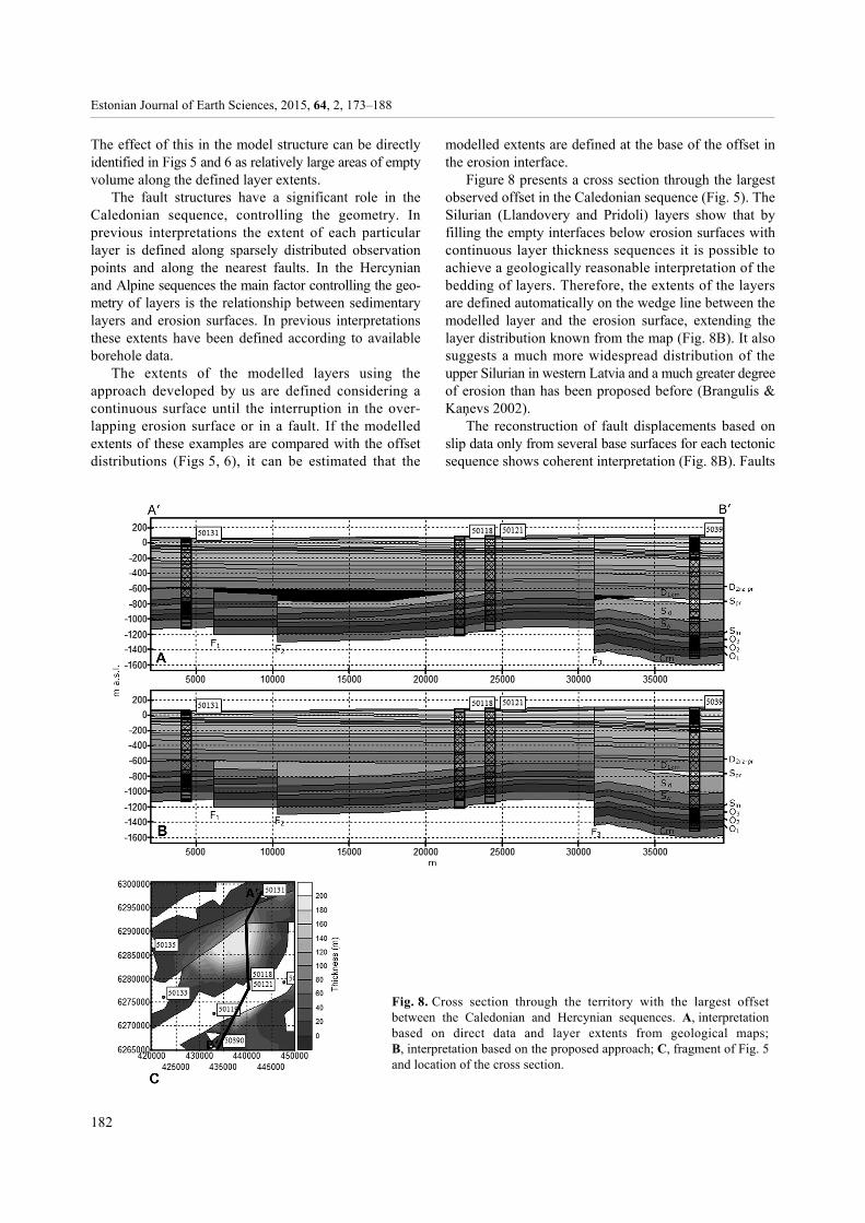
The effect of this in the model structure can be directly identified in Figs 5 and 6 as relatively large areas of empty volume along the defined layer extents.

The fault structures have a significant role in the Caledonian sequence, controlling the geometry. In previous interpretations the extent of each particular layer is defined along sparsely distributed observation points and along the nearest faults. In the Hercynian and Alpine sequences the main factor controlling the geo-metry of layers is the relationship between sedimentary layers and erosion surfaces. In previous interpretations these extents have been defined according to available borehole data.

The extents of the modelled layers using the approach developed by us are defined considering a continuous surface until the interruption in the over-lapping erosion surface or in a fault. If the modelled extents of these examples are compared with the offset distributions (Figs 5, 6), it can be estimated that the

modelled extents are defined at the base of the offset in the erosion interface.

Figure 8 presents a cross section through the largest observed offset in the Caledonian sequence (Fig. 5). The Silurian (Llandovery and Pridoli) layers show that by filling the empty interfaces below erosion surfaces with continuous layer thickness sequences it is possible to achieve a geologically reasonable interpretation of the bedding of layers. Therefore, the extents of the layers are defined automatically on the wedge line between the modelled layer and the erosion surface, extending the layer distribution known from the map (Fig. 8B). It also suggests a much more widespread distribution of the upper Silurian in western Latvia and a much greater degree of erosion than has been proposed before (Brangulis & Kaņevs 2002).

The reconstruction of fault displacements based on slip data only from several base surfaces for each tectonic sequence shows coherent interpretation (Fig. 8B). Faults

Fig. 8. Cross section through the territory with the largest offsetbetween the Caledonian and Hercynian sequences. A, interpretationbased on direct data and layer extents from geological maps;B, interpretation based on the proposed approach; C, fragment of Fig. 5and location of the cross section.


183

were modelled by maintaining non-eroded thickness distribution along the faults, where the slip amplitudes were overtaken from adherent base surfaces. In such a way layer thickness is preserved along faults. However, in some model areas we faced problems expressed as unreasonable thickness variation between base surfaces. A common example is illustrated in Fig. 8A between the Ar–Pr (base of Cm) and O3 layers. While in most part of the cross section the thickness distribution of O3 is analogous, in blocks between the 1st and 2nd faults the thickness is increased. Such problems are reduced through thickness distribution constraints for the affected strata based on borehole data on the coherent bedding of layers (Fig. 8B).

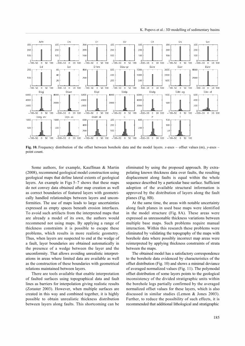
Figure 9 includes the resulting geological model of Latvia. By introducing the surfaces in depositional and erosion surface categories, intersecting and segmenting each layer with faults or overlapping erosion surface, the resulting geometry shows correct topologies and thickness distribution of sedimentary layers. The model structure presents the current geometry of the sedimentary succession and the known fault pattern where it is possible to clearly distinguish major structural features of the Caledonian and Hercynian stages as well as local structures including local highs and depressions. In general, the developed model is consistent with the current understanding of the geological structure of Latvia. Model verification against borehole data The model was built considering only limited borehole data that fully described a particular layer. Due to over-taking the underlying surface by thickness aggregation between layers, the accuracy of the model was verified as an offset between model surfaces and the borehole data. Comparison (Fig. 10) shows that the distribution of the offset is generally normal or near to normal, with a slight asymmetry of values within the 5 m range. Numerically the most important offset with the highest frequency is up to 20 m. The averaged offset distribution of each particular layer is within 3 m (Fig. 11). Analysis indicates multiple reasons for inadequacy that will be described further.

The accuracy of the base surfaces is, however, acceptable (Fig. 10). Good match can be observed for all layers below the Devonian. The largest oscillations are in the layers corresponding to the Upper Devonian–Triassic strata, especially to D3st-el and D3ktl-sk layers with bimodal distribution and strong asymmetry.

The distribution of the averaged normalized offset values of all boreholes do not exceed 2.5 m against modelled surfaces (a in Fig. 11). Offset distribution against boreholes describing the thickness of deeper layers is within 1 m (b in Fig. 11). Systematic increase in

these offsets along the geological section is due to partial summing of the offsets by aggregation of layer thicknesses to the uppermost base surface in points where borehole data describe only part of the geological section. It means that offset against borehole data may occur in the first deepest layer described in the borehole geological log and can be reflected in the whole section.

The offset values against the borehole data that describe only the layer surface (c in Fig. 11) show how reliable the prediction of layer geometry was, as this dataset was not used in modelling. We observed an almost linear relationship between the offsets of borehole data that describe only the surface of the layer and boreholes that were used in modelling. Mostly the offset is about 1–1.5 m greater than the dataset that was used in modelling. Using the largest mismatch, we can directly indicate problematic layers: Sld, D1gr, D1km, D3st-el and D3ktl-sk. In the case of Sld and D1gr, the mismatch is due to insufficient data (Fig. 4). The above-mentioned Devonian layers may also indicate problems associated with incorrectly determined layer boundaries in borehole logs, which has been discussed in similar studies (Lemon & Jones 2003). DISCUSSION The main difficulty within the 3D geological modelling of sedimentary systems is determining the geological boundaries of missing strata. It is difficult to construct spatial geometry with a desired accuracy (Zhu et al. 2012). In this study particular attention has been paid to the two geological processes that have a major role in controlling the geometry of the geological structure in regional scale – faulting and erosion. We considered that the displacement along faults within each sequence can be equal, if not stated otherwise, and the discontinuity of sedimentary layers is possible only in the presence of erosion. Therefore we obtained a tool for controlling basic geometrical relationships between model layers (erosion or onlap) as well as traceability of faults by using thickness constraints of sedimentary layers. That provided a possibility of automatic model building as long as the data describing the thickness distribution of each formation and structural data describing fault locations and displacements along them at least for one surface within the tectonic sequence are available.

The usage of thickness constraints for each sedi-mentary layer allows reducing uncertainties associated with spatially correct definition of layer extents and transferring known fault displacements to the whole sedimentary succession. This approach overcomes limita-tions of the typical modelling procedure by treating these problems jointly.


184

Fig

. 9. 3

D g

eolo

gica

l mod

el o

f L

atvi

a. A

, 3D

vie

w f

rom

sou

th to

nor

th, v

erti

cal e

xagg

erat

ion

1 : 5

0; B

, cro

ss s

ecti

on th

roug

h th

e m

odel

are

a, v

erti

cal e

xagg

erat

ion

1 : 3

0.


185

Some authors, for example, Kauffman & Martin (2008), recommend geological model construction using geological maps that define lateral extents of geological layers. An example in Figs 5–7 shows that these maps do not convey data obtained after map creation as well as correct boundaries of featured layers with geometri-cally handled relationships between layers and uncon-formities. The use of maps leads to large uncertainties expressed as empty spaces beneath erosion interfaces. To avoid such artifacts from the interpreted maps that are already a model of its own, the authors would recommend not using maps. By applying a range of thickness constraints it is possible to escape these problems, which results in more realistic geometry. Thus, when layers are suspected to end at the wedge of a fault, layer boundaries are obtained automatically in the presence of a wedge between the layer and the unconformity. That allows avoiding unrealistic interpret-ations in areas where limited data are available as well as the construction of these boundaries with geometrical relations maintained between layers.

There are tools available that enable interpretation of faulted surfaces using topographical data and fault lines as barriers for interpolation giving realistic results (Zoraster 2003). However, when multiple surfaces are created in this way and combined together, it is highly possible to obtain unrealistic thickness distribution between layers along faults. This shortcoming can be

eliminated by using the proposed approach. By extra-polating known thickness data over faults, the resulting displacement along faults is equal within the whole sequence described by a particular base surface. Sufficient adoption of the available structural information is approved by the distribution of layers along the fault planes (Fig. 8B).

At the same time, the areas with notable uncertainty along fault planes in used base maps were identified in the model structure (Fig. 8A). These areas were expressed as unreasonable thickness variations between multiple base maps. Such problems require manual interaction. Within this research these problems were eliminated by validating the topography of the maps with borehole data where possibly incorrect map areas were reinterpreted by applying thickness constraints of strata between the maps.

The obtained model has a satisfactory correspondence to the borehole data evidenced by characteristics of the offset distribution (Fig. 10) and shows a minimal deviance of averaged normalized values (Fig. 11). The polymodal offset distribution of some layers points to the geological inconsistency of the divided stratigraphic units within the borehole logs partially confirmed by the averaged normalized offset values for these layers, which is also discussed in similar studies (Lemon & Jones 2003). Further, to reduce the possibility of such effects, it is recommended that additional lithological and stratigraphic

Fig. 10. Frequency distribution of the offset between borehole data and the model layers. x-axes – offset values (m), y-axes –point count.


186

Fig. 11. Averaged normalized offset distribution between the modelled surfaces and borehole data: a, all boreholes; b, boreholes with full thicknesses; c, boreholes which reach only the surface of a particular layer.

analysis of borehole logs is undertaken. Some systematic offset increase occurs along the geological column (Fig. 11) due to overtaking of the underlying layer surface by thickness aggregation that leads to certain transfer of the observed offsets. Such a problem appears in points where borehole logs do not describe the whole geological column, but only its upper part. When summing the known thickness to the ‘predicted’ underlying surface topography, the obtained offset is equal to the error of the estimated underlying surface. Due to maximum deviation within 4 m, this effect is insignificant. When estimating the resulting geometry in boreholes describing only the surface of a particular layer (not used in model creation), the maximum offset is within 3 m.

This approach currently handles the interpretation of the missing strata induced only by erosion. It can be efficiently used in regional basin-scale or relatively simple geological conditions. It is possible to automati-cally estimate and deduce the geological genesis of the

missing strata (erosion, and non-deposition) from the stratigraphic column of borehole logs by analysing strati-graphic and lithological records (Zhu et al. 2012). Therefore further work is needed to adapt the mechanism presented by Zhu et al. (2012) to automatic estimation of non-deposition interfaces in borehole logs and to use geological laws controlling these processes within the modelling procedure. That will further allow treating more complex geological structures simultaneously by handling all types of missing strata of different geological environments. CONCLUSION The method presented in this paper is a comprehensive

and automatic treatment of the geological setting, considering it as a sequence of tectonic cycles with similar geological regularities formed by sequential faulting and erosion processes. The method can be applied if stratigraphic intervals from boreholes of the whole geological section and data describing fault locations and displacements are available for at least one surface within the tectonic sequence.

By applying constant thickness to the sedimentary layers it is possible to automatically estimate and allocate the extents of the layers and fault structures keeping consistencies of the missing and adjoining strata. It allows extending viable topography of each layer outside the area described by data where layer extents are defined in the intersection with the over-lying sequence. In the presence of known faults, the displacements along them are automatically trans-ferred to adjacent layers.

The methodology used allows testing alternative interpretations of the chronology of geological events.

The developed 3D geological model highlights coherent interpretation of the geological and structural setting. The extents of the modelled layers overcome limitations of interpretations stored in maps. The neglected areas in map data are reinterpreted by grounding them on known surrounding borehole data and contain geologically and topologically legitimate interpretation.

At the current resolution the model can be further used for different geological studies or serve as a basis for more detailed as well as more regional geological researches.

To extend the proposed approach to deal with more complex geological cases, further work is needed to convert geological laws to modelling concepts that can help to automatically treat the missing strata induced by non-deposition, superposition and compounds of all types.


187

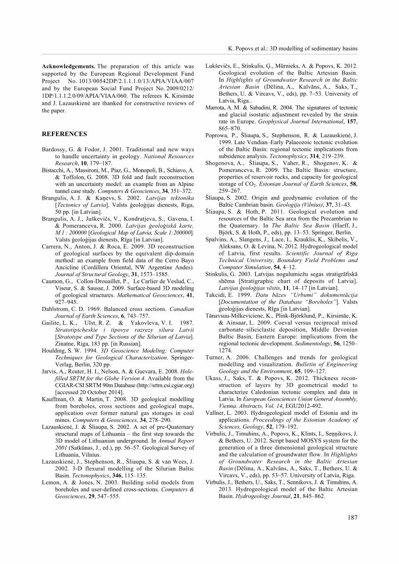
Acknowledgements. The preparation of this article was supported by the European Regional Development Fund Project No. 1013/00542DP/2.1.1.1.0/13/APIA/VIAA/007 and by the European Social Fund Project No. 2009/0212/ 1DP/1.1.1.2.0/09/APIA/VIAA/060. The referees K. Kirsimäe and J. Lazauskienė are thanked for constructive reviews of the paper. REFERENCES Bardossy, G. & Fodor, J. 2001. Traditional and new ways

to handle uncertainty in geology. National Resources Research, 10, 179–187.

Bistacchi, A., Massironi, M., Piaz, G., Monopoli, B., Schiavo, A. & Toffolon, G. 2008. 3D fold and fault reconstruction with an uncertainty model: an example from an Alpine tunnel case study. Computers & Geosciences, 34, 351–372.

Brangulis, A. J. & Kaņevs, S. 2002. Latvijas tektonika [Tectonics of Latvia]. Valsts ģeoloģijas dienests, Riga, 50 pp. [in Latvian].

Brangulis, A. J., Juškevičs, V., Kondratjeva, S., Gavena, I. & Pomeranceva, R. 2000. Latvijas ģeoloģiskā karte, M 1 : 200000 [Geological Map of Latvia, Scale 1:200000]. Valsts ģeoloģijas dienests, Rīga [in Latvian].

Carrera, N., Anton, J. & Roca, E. 2009. 3D reconstruction of geological surfaces by the equivalent dip-domain method: an example from field data of the Cerro Bayo Ancicline (Cordillera Oriental, NW Argentine Andes). Journal of Structural Geology, 31, 1573–1585.

Caumon, G., Collon-Drouaillet, P., Le Carlier de Veslud, C., Viseur, S. & Sausse, J. 2009. Surface-based 3D modeling of geological structures. Mathematical Geosciences, 41, 927–945.

Dahlstrom, C. D. 1969. Balanced cross sections. Canadian Journal of Earth Sciences, 6, 743–757.

Gailite, L. K., Ulst, R. Z. & Yakovleva, V. I. 1987. Stratotipicheskie i tipovye razrezy silura Latvii [Stratotype and Type Sections of the Silurian of Latvia]. Zinatne, Riga, 183 pp. [in Russian].

Houlding, S. W. 1994. 3D Geoscience Modeling; Computer Techniques for Geological Characterization. Springer-Verlag, Berlin, 320 pp.

Jarvis, A., Reuter, H. I., Nelson, A. & Guevara, E. 2008. Hole-filled SRTM for the Globe Version 4. Available from the CGIAR-CSI SRTM 90m Database (http://srtm.csi.cgiar.org) [accessed 20 October 2014].

Kauffman, O. & Martin, T. 2008. 3D geological modelling from boreholes, cross sections and geological maps, application over former natural gas storages in coal mines. Computers & Geosciences, 34, 278–290.

Lazauskienė, J. & Šliaupa, S. 2002. A set of pre-Quaternary structural maps of Lithuania – the first step towards the 3D model of Lithuanian underground. In Annual Report 2001 (Satkūnas, J., ed.), pp. 56–57. Geological Survey of Lithuania, Vilnius.

Lazauskienė, J., Stephenson, R., Šliaupa, S. & van Wees, J. 2002. 3-D flexural modelling of the Silurian Baltic Basin. Tectonophysics, 346, 115–135.

Lemon, A. & Jones, N. 2003. Building solid models from boreholes and user-defined cross-sections. Computers & Geosciences, 29, 547–555.

Lukševičs, E., Stinkulis, Ģ., Mūrnieks, A. & Popovs, K. 2012. Geological evolution of the Baltic Artesian Basin. In Highlights of Groundwater Research in the Baltic Artesian Basin (Dēlina, A., Kalvāns, A., Saks, T., Bethers, U. & Vircavs, V., eds), pp. 7–53. University of Latvia, Riga..

Marrota, A. M. & Sabadini, R. 2004. The signatures of tectonic and glacial isostatic adjustment revealed by the strain rate in Europe. Geophysical Journal International, 157, 865–870.

Poprowa, P., Šliaupa, S., Stephenson, R. & Lazauskienė, J. 1999. Late Vendian–Early Palaeozoic tectonic evolution of the Baltic Basin: regional tectonic implications from subsidence analysis. Tectonophysics, 314, 219–239.

Shogenova, A., Šliaupa, S., Vaher, R., Shogenov, K. & Pomeranceva, R. 2009. The Baltic Basin: structure, properties of reservoir rocks, and capacity for geological storage of CO2. Estonian Journal of Earth Sciences, 58, 259–267.

Šliaupa, S. 2002. Origin and geodynamic evolution of the Baltic Cambrian basin. Geologija (Vilnius), 37, 31–43.

Šliaupa, S. & Hoth, P. 2011. Geological evolution and resources of the Baltic Sea area from the Precambrian to the Quaternary. In The Baltic Sea Basin (Harff, J., Björk, S. & Hoth, P., eds), pp. 13–53. Springer, Berlin.

Spalvins, A., Slangens, J., Lace, I., Krauklis, K., Skibelis, V., Aleksans, O. & Levina, N. 2012. Hydrogeological model of Latvia, first results. Scientific Journal of Riga Technical University, Boundary Field Problems and Computer Simulation, 54, 4–12.

Stinkulis, G. 2003. Latvijas nogulumiežu segas stratigrāfiskā shēma [Stratigraphic chart of deposits of Latvia]. Latvijas ģeoloģijas vēstis, 11, 14–17 [in Latvian].

Takcidi, E. 1999. Datu bāzes “Urbumi” dokumentācija [Documentation of the Database “Boreholes”]. Valsts ģeoloģijas dienests, Rīga [in Latvian].

Tänavsuu-Milkeviciene, K., Plink-Björklund, P., Kirsimäe, K. & Ainsaar, L. 2009. Coeval versus reciprocal mixed carbonate–siliciclastic deposition, Middle Devonian Baltic Basin, Eastern Europe: implications from the regional tectonic development. Sedimentology, 56, 1250–1274.

Turner, A. 2006. Challenges and trends for geological modelling and visualization. Bulletin of Engineering Geology and the Environment, 65, 109–127.

Ukass, J., Saks, T. & Popovs, K. 2012. Thickness recon-struction of layers by 3D geometrical model to characterize Caledonian tectonic complex and data in Latvia. In European Geosciences Union General Assembly, Vienna. Abstracts, Vol. 14, EGU2012-492.

Vallner, L. 2003. Hydrogeological model of Estonia and its applications. Proceedings of the Estonian Academy of Sciences, Geology, 52, 179–192.

Virbulis, J., Timuhins, A., Popovs, K., Klints, I., Seņņikovs, J. & Bethers, U. 2012. Script based MOSYS system for the generation of a three dimensional geological structure and the calculation of groundwater flow. In Highlights of Groundwater Research in the Baltic Artesian Basin (Dēlina, A., Kalvāns, A., Saks, T., Bethers, U. & Vircavs, V., eds), pp. 53–57. University of Latvia, Riga.

Virbulis, J., Bethers, U., Saks, T., Sennikovs, J. & Timuhins, A. 2013. Hydrogeological model of the Baltic Artesian Basin. Hydrogeology Journal, 21, 845–862.


188

Wu, Q., Xu, H. & Zou, X. 2005. An effective method for 3D geological modeling with multi-source data integration. Computers & Geosciences, 31, 35–43.

Zhu, L., Zhang, C., Li, M., Pan, X. & Sun, J. 2012. Building 3D solid models of sedimentary stratigraphic systems

from borehole data: an automatic method and case studies. Engineering Geology, 127, 1–13.

Zoraster, S. 2003. A surface modeling algorithm designed for speed and ease of use with all petroleum industry data. Computers & Geosciences, 29, 1175—1182.

Settebasseinide 3D modelleerimine Balti basseini keskosa (Läti) näitel

Konrāds Popovs, Tomas Saks ja Jānis Jātnieks

On uuritud settebasseinide geoloogiliste struktuuride modelleerimist iseõppiva poolautomaatse algoritmiga, milles mudeli elementide (settekihtide ja struktuuride) geomeetrilised suhted määratakse automatiseeritult. Mudel eeldab, et settebasseini läbilõige on moodustunud järjestikuste settimise (settekihtide ladestumise), tektooniliste murrangute tekkimise ja erosioonisündmuste tulemusena. Selline lähenemine võimaldab modelleerida settebasseinide geoloo-gilise ehituse kujunemist ka siis, kui settekihtide leviku, paksuste ja läbistavate murrangute kohta ei ole piisavalt andmeid kogu basseini ulatuses. Uurimuses on rakendatud mudelit Balti basseini keskosa (Läti) setteläbilõike geo-loogiliste struktuuride interpreteerimiseks.

a comprehensive approach to the 3d geological modelling of ... · a comprehensive approach to the...

Documents