a compilation of parameters for ecosystem dynamics models ... · a compilation of parameters for...
TRANSCRIPT

CCAMLR Science, Vol. 14 (2007): 1–25
A COMPILATION OF PARAMETERS FOR ECOSYSTEM DYNAMICS MODELS OF THE SCOTIA SEA – ANTARCTIC PENINSULA REGION
S.L. Hill , K. Reid and S.E. ThorpeBritish Antarctic Survey
Natural Environment Research CouncilHigh Cross, Madingley Road
Cambridge CB3 0ETUnited Kingdom
Email – [email protected]
J. HinkeSouthwest Fisheries Science Center
NOAA FisheriesAntarctic Ecosystem Research Division
8604 La Jolla Shores DriveLa Jolla, CA 92037, USA
G.M. WattersSouthwest Fisheries Science Center
NOAA FisheriesProtected Resources Division
1352 Lighthouse AvenuePacifi c Grove, CA 93950, USA
Abstract
Expansion of the krill fi shery in the Scotia Sea–Antarctic Peninsula region beyond the current operational catch limit requires the development and assessment of methods for subdividing the precautionary catch limit amongst smaller spatial units. This paper compiles parameters for use in the ecosystem dynamic models that are needed to assess these methods. These parameters include life history and krill consumption parameters for the fi sh, whale, penguin and seal species that feed on krill in this region. Maximum krill transport rates are also derived from the OCCAM global ocean circulation model. This parameter set, like most others, is associated with considerable uncertainty, which must be taken into account when it is used. The sources, assumptions and calculations at every stage of the compilation process are therefore detailed, and plausible limits for parameter values are provided where possible. The results suggest that fi sh are the major krill consumers in all SSMUs, with perciform fi sh taking as much krill as whales, penguins and fur seals combined and myctophid fi sh taking double that amount. However, estimates of krill consumption per unit predator biomass suggest that this is an order of magnitude higher in penguins and seals than in whales and fi sh.
Résumé
L’expansion de la pêcherie de krill de la région de la mer du Scotia–péninsule antarctique, au-delà de la limite de capture actuellement en vigueur, nécessite la mise au point et l’évaluation de méthodes de subdivision de la limite de précaution des captures en unités spatiales plus petites. Le présent document dresse la liste des paramètres à utiliser dans les modèles de la dynamique de l’écosystème, qui sont nécessaires pour évaluer ces méthodes. Ces paramètres comprennent, entre autres, les paramètres du cycle biologique et de la consommation de krill des espèces de poissons, de cétacés, de manchots et d’otaries qui se nourrissent de krill dans la région. Les fl ux maximum de krill proviennent du modèle OCCAM de circulation océanique globale. Cet ensemble de paramètres, comme bien d’autres, est entouré d’une incertitude considérable, dont il faut tenir compte lors de son utilisation. Les sources, les hypothèses et les calculs, à chaque étape du processus de compilation, sont donc détaillés et des limites plausibles sont fournies lorsque cela est possible pour les valeurs paramétriques. Les résultats laissent penser que les poissons sont les principaux consommateurs de krill dans toutes les SSMU, les poissons perciformes en ingurgitant autant que les cétacés, les manchots et les otaries réunis et les poissons myctophidés, le double de cette quantité. Les estimations de la consommation de krill par unité de biomasse de prédateurs semblent néanmoins indiquer que celle des manchots et des otaries est supérieure à celle des cétacés et des poissons, la différence étant de l’ordre d’un facteur 10.

Hill et al.
2
Introduction
Expansion of the krill fi shery in the Scotia Sea–Antarctic Peninsula region (FAO Statistical Area 48) beyond the current operational catch limit requires the development and assessment of meth-ods for subdividing the precautionary catch limit among smaller spatial units. CCAMLR’s Working Group on Ecosystem Monitoring and Management (WG-EMM) has defi ned such small-scale manage-ment units (SSMUs) and proposed a set of candidate options for subdivision of the catch limit (Hewitt et al., 2004a). The evaluation of these options will involve simulating their effects on krill and its predators using ecosystem dynamics models.
Such models must be spatially resolved at least to the scale of SSMUs and must represent krill and predator populations within these areas. WG-EMM has also recognised that the temporal resolution of such models must distinguish at least two sea-sons (summer and winter) to represent differences between SSMUs in the temporal overlap of fi shing and predator breeding (SC-CAMLR, 2005). In order to represent the population dynamics of the focal species (krill and its dependent predators), such models will need information on key life history and population parameters. The functions repre-senting the interactions between species must also be parameterised. The models must also account for uncertainties associated with the structure and
Резюме
Превышение крилевым промыслом в районе моря Скотия – Антарктического п-ова рамок существующего рабочего ограничения на вылов требует разработки и оценки методов подразделения предохранительного ограничения на вылов между более мелкими пространственными единицами. В данной статье собраны необходимые для оценки этих методов параметры, применяемые в динамических моделях экосистемы. Эти параметры включают данные о жизненном цикле и потреблении криля для видов рыб, китов, пингвинов и тюленей, которые питаются крилем в этом регионе. Максимальная скорость переноса криля также приводится по модели глобальной циркуляции океана OCCAM. Для этого набора параметров, как и для большинства других, характерна значительная неопределенность, которую следует учитывать при его использовании. В связи с этим, на каждом этапе компиляционного процесса источники, допущения и расчеты детализируются и, по возможности, приводятся вероятные пределы значений параметров. Согласно результатам, основным потребителем криля во всех SSMU является рыба, причем рыбы отряда окунеобразных съедают столько же криля, сколько киты, пингвины и тюлени вместе взятые, а миктофиды – вдвое больше. Однако оценки потребления криля на единицу биомассы хищников говорят о том, что у пингвинов и тюленей этот показатель на порядок выше, чем у китов и рыбы.
Resumen
La expansión de la pesquería de kril en la región del Mar de Escocia–Península Antártica más allá del límite operacional de captura actualmente vigente, requiere de la formulación y evaluación de métodos para subdividir el límite de captura precautorio en áreas más pequeñas. Este trabajo compila parámetros para las simulaciones de la dinámica del ecosistema requeridas en la evaluación de estos métodos. Los parámetros incluyen el ciclo de vida y el consumo de kril de las especies de peces, cetáceos, pingüinos y pinnípedos que se alimentan del recurso en esta región. Las tasas máximas de transporte de kril también se derivan del modelo OCCAM de circulación oceánica global. La magnitud de la incertidumbre inherente a este conjunto de parámetros, al igual que la de muchos otros, es considerable y debe ser tomada en cuenta al utilizarlo. Por lo tanto, se han detallado las fuentes, suposiciones y cálculos efectuados en todas las etapas de la compilación, y en la medida de lo posible, se proporcionaron los márgenes verosímiles de los valores de los parámetros. Los resultados indican que los peces son los mayores consumidores de kril en todas las UOPE, y de éstos, los peces perciformes consumen tanto kril como el consumido colectivamente por ballenas, pingüinos y lobos fi nos, y los peces mictófi dos consumen el doble de esta cantidad. No obstante, las estimaciones del consumo de kril por unidad de biomasa de los depredadores indican que en el caso de los pingüinos y pinnípedos, dicho consumo es un orden de magnitud mayor que el de las ballenas y los peces.
Keywords: small-scale management unit, Scotia Sea, krill–predator–fi shery model, life history, krill consumption, ecosystem model, CCAMLR

3
Parameters for Scotia Sea ecosystem dynamics models
functioning of the ecosystem. One of the key uncer-tainties concerns the infl uence of advection on the local dynamics of krill (Hill et al., 2006).
This paper compiles and derives key parame-ters for the fi sh, whale, penguin and seal predators of krill. It is intended for general use in modelling studies of krill and its dependent predators in the Scotia Sea–Antarctic Peninsula region. However, it is particularly relevant to the ecosystem dynamics models presented at two WG-EMM workshops on Management Procedures (SC-CAMLR, 2005, 2006). These models represent the dynamics of preda-tor populations with delay-difference equations in which individuals recruit to the adult popula-tion at the age of fi rst breeding. The models are similar in their treatment of krill dynamics: the krill–predator–fi shery model (KPFM), developed by Dr G. Watters (NOAA Fisheries, USA) and col-leagues (at BAS, UK and NOAA Fisheries, USA), models krill numbers but assumes a constant mean mass, whereas the spatial multi-species operat-ing model (SMOM) developed by Dr É. Plagányi and Prof. D. Butterworth (University of Cape Town, South Africa) directly models krill biomass. Although the population demographic structure and individual growth of krill are potentially important characteristics, they are not discussed in more detail because they are not explicitly con-sidered in these models. As these models consider a limited number of predator taxa, a way of com-bining parameters for different species to repre-sent ‘generic’ predators is suggested. The predator parameters derived here, their symbols, and their relevance in the KPFM are listed in Table 1.
This paper also provides information on SSMUs and historical catch, which is necessary for mod-elling the catch allocation options in Hewitt et al. (2004a). Furthermore, it derives maximum krill transport rates between SSMUs to defi ne an upper bound on this important source of uncer-tainty. The intention is to provide a parameter set that best refl ects current knowledge of the system. However, this knowledge is far from complete. Details are therefore provided of sources, methods and assumptions, which serve as an audit trail. Plausible limits are also estimated for parameter values where possible. This is intended to provide the information required to stimulate debate and research that will challenge current assumptions and address important gaps in this knowledge.
Approach: parameters, uncertainty and model inputs
The parameter estimates are derived from four main sources: the published literature; direct
calculation when data were available; model out-put in the case of the krill transport parameters; and, fi nally, assumptions based on similar spe-cies, expert opinion or unpublished studies when values were unavailable from the other sources. Assumptions based on similar species were made only when they were necessary to derive the parameters in Tables 14 and 15. The parameters ρk,j and αk,j for fi sh were not included in these tables as they would have been based largely on such assumptions.
Parameters were derived for two seasons, cor-responding to the six months from 1 October (sum-mer) and the six months from 1 April (winter). However, natural mortality rate estimates tend to be annual rather than seasonal. Lifetime aver-aged annual rates (indicated by the symbol μ) were divided by 2 to obtain estimates of Mk,j,s. The deri-vation of the krill transport parameters is described in a self-contained section of the main text and fre-quently used equations are described in the present section. However, the derivation of many predator parameters required specifi c calculations, which are described in accompanying notes (following ‘References’), along with details of the data sources used.
Uncertainty is dealt with by reporting minimum and maximum plausible values for parameters alongside average values. These limits are either the extremes of reported values or the 95% confi dence intervals of estimates. Values shown without limits indicate that there was insuffi cient information to assess this uncertainty.
αk,j was calculated depending on the available information as follows:
max max 1 Ar e−μα = + − (1a)
min . Je− μ ρα = Λ (1b)
where μA and μJ are the adult and pre-recruit annual mortality rates, rmax is the maximum observed rate of population increase and Λ is the observed number of live offspring produced per breeding adult per year.
Derived krill demand estimates are for the adult portion of the relevant populations (except for whales, where separate abundance estimates were not available for adults). The demand of adults for-aging to feed their offspring is included, but the demand of independently feeding juveniles is not.
In compiling KPFM parameters, four predator taxa were considered: baleen whales, seals, pen-guins and fi sh. Each of these groups is composed

Hill et al.
4
of several species in the Scotia Sea–Antarctic Peninsula region, and the members of some groups, particularly fi sh, have very different char-acteristics. Parameters for generic members of each group were calculated as averages weighted by the krill consumption of the initial population of each species within the group. The basic calculation for a generic predator was:
, ,1
,
,1
l
i j i ji
k j l
i ji
D X
XD
=
=
=∑
∑ (2)
where ,k jX is the generic value of parameter X for taxon k, Xi,j is its value for the i’th of l species in taxon k in SSMU j, and Di,j is the total annual krill consumption of species i in SSMU j.
SSMU areas
The basic spatial unit of the current parameter set is the SSMU. The KPFM includes additional spatial units, known as ‘boundary areas’, that bor-der these management units and represent the spa-tial boundaries of the model. This parameterisation
considers three boundary areas corresponding to areas in the Bellingshausen Sea, the Drake Passage and the Weddell Sea respectively (Figure 1). These boundary areas are essentially boxes fi tted around the greatest distances that particles originating in the SSMUs could travel over six months, and the greatest distances from which particles could reach the SSMUs in six months. These distances were estimated by tracking particle advection in model velocity fi elds on a horizontal grid of resolution 0.25° latitude by 0.5° longitude (see next section).
The area within each SSMU was provided by the CCAMLR Secretariat and was calculated from the global sea-fl oor topography database of Smith and Sandwell (1997). Boundary areas were calculated from the GEBCO bathymetric database (IOC, IHO and BODC, 2003). For the purposes of this paper, the marine habitat in each SSMU is divided into two types: waters with depth ≤500 m are defi ned as ‘shelf’ areas and waters deeper than 500 m were defi ned as ‘off-shelf’ areas. Basic information on each SSMU, including the total krill catch from 1988 to 2002, is given in Table 2.
Figure 1: The Scotia Sea–Antarctic Peninsula region, showing the SSMUs (names in Table 2), boundary areas and sites mentioned in the text.
Boundary area 1
Boundary area 2
Boundary area 3

5
Parameters for Scotia Sea ecosystem dynamics models
Krill transport
The exact role of advective transport on local krill dynamics is uncertain. The plausible limits on this uncertainty identifi ed by WG-EMM (SC-CAMLR, 2006) were no krill transport between SSMUs ver-sus the transport of krill as passive drifters. A more extreme scenario, which cannot be discounted but was not considered, would involve krill swim-ming with the currents. Parameters for the passive-drifter hypothesis were derived by tracking parti-cle movements in velocity fi elds output from the ocean circulation model of the Ocean Circulation Climate Advanced Modelling Project (OCCAM). This model has 66 vertical levels, with a horizontal resolution of 0.25º by 0.25º (Coward and de Cuevas, 2005). A subset of output was used. This covered the model domain 45º–75ºS 100º–20ºW and the upper 100 m of the water column (upper 14 model levels). For each calendar month, a depth-weighted mean velocity fi eld was calculated over a 19-year run of this model (1985 to 2003). Prior to use in the advection scheme, the monthly mean velocity fi elds were modifi ed according to Killworth (1996) to avoid errors associated with linear interpolation between mean fi elds.
The particles were advected using a second-order Runge-Kutta advection scheme, following Murphy et al. (2004). The advection scheme used a timestep of 0.1 day and did not explicitly include diffusion. The scheme applies a no-slip boundary condition at coasts and, once particles leave the model domain, they take no further part in the simulations. Particles were released on a regular grid within predefi ned areas of SSMUs and bound-ary areas, with a resolution of 0.25º latitude by 0.5º longitude. The particles were advected through the velocity fi elds for 183 days (~6 months) begin-ning on either 1 October or 1 April to derive the summer and winter transport rates respectively.
The instantaneous transport rate between model spatial units (SSMUs and boundary areas) was cal-culated as follows:
,, ln 1 m n
m n mm
v ≠θ⎛ ⎞
= − −⎜ ⎟θ⎝ ⎠
(3a)
, 0m n mv = = (3b)
where mθ is the number of particles released in area m at the beginning of the advection period and ,m nθ is the number of these particles that were found in area n at the end of the period. The resulting summer and winter matrices are given in Tables 3 and 4.
Krill mean mass
The mean body mass of individual krill caught in nets during the CCAMLR 2000 Krill Synoptic Survey of Area 48 was calculated from data sup-plied by Dr V. Siegel (Sea Fisheries Institute, Hamburg, Germany). The overall mean mass was 0.46 g, but there was considerable between-haul variability in mean mass (range: 0.11 to 1.27 g, SD: 0.31 g, n = 93).
Fish
The krill-eating fi sh fauna are composed largely of demersal members of the order Perciformes (mainly families Nototheniidae and Channichthyidae, the icefi sh) and pelagic mem-bers of the family Myctophidae. The assumption was made that off-shelf areas are populated by a generic myctophid and that shelf areas are popu-lated by a generic perciform. Generic parameters were estimated separately for these two taxa, and then combined according to estimated krill demand within SSMUs to estimate parameters for generic fi sh (equation 2). The body mass and mor-tality rates of these two taxa are very different, so the characteristics of generic fi sh varied with the relative area of the two habitats in each SSMU.
Although Kock (1992) reported the results of virtual population analyses (VPAs) for some Scotia Sea fi sh species, no stock-recruit information is available for relevant myctophid species. Also, life history information is scarce for many of the important krill-consuming fi sh. Therefore, the two parameters relating to recruitment (ρk,j and αk,j) were not estimated for fi sh. Uncertainty was not evaluated for many of the derived parameters as it is unlikely that the limited available data fully refl ect the spatial and temporal variability in fi sh population sizes.
Myctophid fi sh
Pusch et al. (2004) provided biomass density and krill consumption estimates for myctophids based on a limited study on the shelf slope near King George Island, suggesting that Gymnoscopelus nicholsi and Electrona antarctica are responsible for the majority of krill consumption by myctophids.
*, ,k j sQ and Pk,j estimates were based on data from
Pusch et al. (2004) for these species (Notes F1 to F6; Tables 5 and 7). μ values for similar species were obtained from Kock (1992).

Hill et al.
6
Perciform fi sh
*, ,k j sQ and Pk,j estimates for perciform fi sh were
based on estimates of abundance and krill con-sumption from extensive trawl surveys in three areas of the Scotia Sea, reported in Kock (1985) (Note F7; Table 6). Life history parameters for per-ciforms were based on Champsocephalus gunnari, which was the main krill consumer identifi ed by Kock (1985). The μ for perciforms in Table 7 is the average of the range of values quoted for C. gunnari at South Georgia in Kock (1992). Growth param-eters for C. gunnari from Agnew et al. (1998) were used to estimate mean mass, which, in turn, was used to estimate Pk,j from biomass density data (Note F8).
Seals
Only one seal species was considered: the Antarctic fur seal (Arctocephalus gazella). There are considerable differences between the sexes of this species, in characteristics including age-at-fi rst-reproduction, body size and mortality rate (Table 9). In addition, a substantial proportion of adult females do not breed each year, and these non-breeders are likely to have lower food require-ments than those nursing pups. Average character-istics were therefore calculated across these three different groups of adult fur seals. This required the construction of a simple demographic projec-tion to calculate sex ratios (Note S2; Table 8).
The life history parameters used in this demo-graphic projection and to calculate Mk,j,s and ρk,j were obtained from McCann and Doidge 1987; Boyd et al. (1995); Wickens and York (1997); Boyd (2002b) and Goebel et al. (2006). The population growth rate reported by Payne (1977) was used to calculate αmax.
Pk,j estimates were obtained from SC-CAMLR (2002). This lists the position of fur seal breed-ing colonies and the estimated number of breed-ing females in each colony. These colonies were assigned to the SSMUs they were located in and the abundance estimates were scaled up to include males and non-breeding females.
Estimates of annual krill requirements were taken from Boyd (2002a) (see Note S3). These were converted to *
, ,k j sQ estimates using the arbitrary ratios in Table 9. The fi rst-season requirement of pups was added to that of breeding females.
Penguins
Generic penguin parameters were calculated using specifi c parameters for Adélie (Pygoscelis adeliae), chinstrap (P. antarctica), gentoo (P. papua) and macaroni (Eudyptes chrysolophus) penguins. Abundance data from SC-CAMLR (2002) (derived largely from Woehler, 1993), were supplemented with data for four additional Adélie penguin colonies, provided by the CCAMLR Secretariat (Table 10), and Pk,j was calculated using these data.
Mk,j,s, ρk,j and αk,j were calculated from basic life-history parameters in Williams (1995) and from the monitoring programs of BAS at Bird Island and Signy Island and the US Antarctic Marine Living Resources Program at Copacabana Beach, Admiralty Bay, King George Island. However, arbitrary values were used for juvenile μ and the proportion of non-breeding adults for all species (Notes P1 to P3). An arbitrary value was also used for the adult μ of chinstrap penguins.
*, ,k j sQ for Adélie, chinstrap and gentoo pen-
guins were calculated from the krill consumption estimates and population structures in Croll and Tershy (1998) (Note P4). An arbitrary 1:1 sex ratio was assumed for the adult population and the indi-vidual krill requirements of adults were arbitrarily assumed to be constant throughout the year. Chick requirements during the breeding season were added to those of adults (Notes P5 and P6). The annual krill demand estimates for macaroni pen-guins in Boyd (2002a) were used to obtain *
, ,k j sQ for this species (Note P6; Table 12).
Whales
Reilly et al. (2004) estimated the abun-dance and krill requirements of fi n (Balaenoptera physalus), humpback (Megaptera novaeangliae), minke (B. bonaerensis) and southern right whales (Eubalaena australis) as well as the overall abun-dance of ‘large baleen’ whales including hump-back, fi n, southern right, blue (B. musculus) and sei (B. borealis) whales in strata corresponding to the Scotia Sea and Antarctic Peninsula regions. Branch and Butterworth (2001) reported the number of pods, by species, sighted on surveys of larger strata that also overlap these areas. These two data sources were used to calculate Pk,j limits for the spe-cies listed by Reilly et al. (2004) (Note W1). There was very good correspondence between these two data sources, with the Reilly et al. (2004) data estimating total whale abundance as (mean and 95% confi dence intervals) 36 069 (9 831–42 274) and the Branch and Butterworth (2001) data estimating 34 145 (13 163–52 380).

7
Parameters for Scotia Sea ecosystem dynamics models
These data, together with life history param-eters from Laws (1977), Boness et al. (2002) and unpublished studies (Notes W4 and W5) were used to estimate separate generic parameters for the Scotia Sea and Antarctic Peninsula regions on the arbitrary assumption that whale fauna was comparable between the individual SSMUs in each region (Notes W1 to W8; Table 13).
KPFM input parameters and demand estimates
The parameters compiled here were used to derive KPFM input parameters for four generic predators representing fi sh, whales, penguins and seals (Tables 14 and 15). Except where the notes indicate otherwise, these values are based on aver-age component parameters. The maximum annual krill demand, by predator type, per SSMU implied by the KPFM parameters was also estimated (Table 16). This suggests that fi sh are the major krill consumers in all SSMUs, with perciform fi sh tak-ing as much krill as whales, penguins and fur seals combined and myctophid fi sh taking double that amount. Of the air-breathing predators, penguins have the highest demand. Krill consumption per unit predator biomass was also calculated for each of the generic predator taxa. These estimates are not strictly comparable between taxa (see caveats in the legend to Table 16). However, they suggest an enormous range in consumption to biomass ratios from 2 year–1 in whales to 103 year–1 in penguins.
Discussion
This paper compiles information about a number of species, taken from studies at a range of spatial and temporal scales, into a coherent and spatially resolved view of the regional krill-based food web. This can be used to parameterise popu-lation dynamic models for krill-dependent preda-tors based on delay-difference equations, and it should be a useful reference for other analyses of the system at the regional and SSMU scales. This paper also illustrates a practical method for linking output from the OCCAM ocean circulation model to ecosystem dynamics models in the form of trans-port rates between SSMUs.
Tables 14 and 15 provide many of the input parameters required for KPFM.
Sets of plausible limit values are also available on request from the authors. However, there are a number of KPFM input parameters that have not been derived here.
These parameters concern the distribution of predator foraging effort amongst SSMUs other than the one in which the predators breed, and the form of functional relationships (describing the functional and numerical response of preda-tors and the stock-recruit relationship for krill). It will be necessary to make assumptions about these parameter values and their associated uncertainty, and the onus is on the analyst to justify and test these assumptions.
The complexity and scale of the system and its dynamics ensure that it will be impossible to ever describe it fully. Therefore, while the parameters used here summarise the best available information about selected krill predators, they should not be considered defi nitive. This paper provides a clear audit-trail of its sources, methods and assumptions to facilitate the necessary scrutiny. It also represents uncertainty, where possible, by reporting plausi-ble limits for parameter values. It is important to remember that, where such limits are not shown, it does not imply certainty in the parameter esti-mate, but rather a lack of information with which to quantify uncertainty. As an understanding of uncertainty is particularly important in evaluating management options, the remainder of this discus-sion highlights some additional uncertainties asso-ciated with the current parameter set.
While the published literature provides a repos-itory of knowledge, it is not always current. This is particularly true for populations whose size changes rapidly or where new information has not yet been included in published population size estimates. The values used here for Antarctic fur seals at South Georgia are considered to be unreli-able (J. Forcada, BAS, pers. comm.) and those for humpback whales in the Scotia Sea are consid-ered to be underestimates (A. Martin, BAS, pers. comm.), although no revised estimates have been published.
Empirical values have been compiled from a variety of studies focusing on different, but lim-ited, temporal and spatial scales. These studies inevitably represent a ‘snapshot’ of conditions that might not apply to other scales. In particular, the abundance estimates for the various predators may represent different states in the system’s dynam-ics. Also, myctophid fi sh diets and densities from the shelf slope near King George Island have been extrapolated to all waters deeper than 500 m. Since this study identifi es myctophids as the taxon that consumes most krill, there is a particular need to examine the uncertainty associated with this extra-polation. Furthermore, the fi eld studies on which demand estimates are based usually consider time
Hill et al.
8
periods of less than one year, which are usually in the summer months. Extrapolating from these to other parts of the year also introduces uncertainty. In particular, there is a risk of bias in the penguin demand estimates presented here. The extrapola-tions and assumptions of contemporaneousness made in this study do not imply that the system is homogenous and stable at the relevant scales. They merely highlight a lack of suitable information on its heterogeneity and dynamics.
The parameters presented here concern the ‘krill-dependent’ penguins and seals that are an important focus of the CCAMLR Ecosystem Monitoring Program, the baleen whales and fi sh. This combination is intended to represent current interest in the conservation of endothermic preda-tors and the maintenance of viable fi sh stocks, and to capture important sources of krill consumption. However, this is not a comprehensive survey and other potentially important species, such as crab-eater seals and squid, have not been included as there are few data to assess their abundance and krill requirements. Also, this compilation does not include demand estimates for independent juve-niles of the species considered, which are likely to be substantial.
There are a number of other issues: (i) different whale species may have very different patterns of habitat use and baleen whale distribution might therefore differ from the assumptions presented here; (ii) breeding and non-breeding members of the same species also have different spatial dis-tributions, so the total adult size may not always scale linearly with the breeding population size; (iii) model estimates of krill demand are sensitive to their assumptions; and (iv) the spatial and tem-poral resolution of these parameters will result in some loss of information compared to fi ner scales. For example, the transport matrices imply trans-port between non-adjacent SSMUs with no infor-mation on the intermediate SSMUs that particles passed through.
The estimates of krill demand must be inter-preted in the light of the above caveats, but they suggest that krill demand outstrips estimated bio-mass, highlighting the uncertainty associated with many of these estimates.
Conclusion
This compilation of parameter values is intended for use in ecosystem dynamic models to support the management of the krill fi shery in Area 48. These parameter values are based on a combination of empirical data, published models,
informed estimates and some arbitrary, but clearly stated, assumptions. Consequently, there are many uncertainties associated with these parameters, which must be taken into account when they are used. The KPFM is designed to investigate the implications of differing assumptions and parame-ter values and it is therefore recommend that full use be made of this facility.
Myctophid fi sh appear to be the main krill con-sumers of the taxa considered, but the myctophid abundance estimates are particularly uncertain. This suggests that priority should be given to reducing this uncertainty and investigating its implications for krill management.
Acknowledgements
We have been greatly aided in this compila-tion by advice and information from many people including Eric Appleyard, Bas Beekmans, Anabela Brandão, Doug Butterworth, Martin Collins, Mike Dunn, Greg Donovan, Jaume Forcada, Tony Martin, Aileen Miller, David Ramm, Sarah Robinson, Volker Siegel, Iain Staniland, Wayne Trivelpiece and mem-bers of WG-EMM. We also thank the OCCAM team at the National Oceanography Centre, Southampton, UK, for making the OCCAM out-put readily available, Karl-Herman Kock and his publishers for permission to reproduce the data in Table 6 and Peter Fretwell for producing Figure 1. Some of this work was supported by NSF grant #0443751 to Wayne and Sue Trivelpiece and George Watters. Additional support was also provided to Jefferson Hinke and George Watters by the Lenfest Ocean Program at the Pew Charitable Trusts.
References
Agnew, D.J., I. Everson, G.P. Kirkwood and G.B. Parkes. 1998. Towards the development of a management plan for mackerel icefi sh (Champsocephalus gunnari) in Subarea 48.3. CCAMLR Science, 5: 63–77.
Boness, D.J., P.J. Clapham and S.L. Mesnick. 2002. Life history and reproductive strategies. In: Hoelzel, R. (Ed.). Marine Mammal Biology. Blackwell Publishing, Oxford: 278–324.
Boyd, I.L. 2002a. Estimating food consumption of marine predators: Antarctic fur seals and maca-roni penguins. J. Appl. Ecol., 39 (1): 103–119.

9
Parameters for Scotia Sea ecosystem dynamics models
Boyd, I.L. 2002b. Pinniped life history. In: Perrin, W., B. Wursig and J. Thewissen (Eds). Encyclopedia of Marine Mammals. Academic Press/Elsevier Science.
Boyd, I.L., J.P. Croxall, N.J. Lunn and K. Reid. 1995. Population demography of Antarctic fur seals: the costs of reproduction and implications for life-histories. J. Anim. Ecol., 64 (4): 505–518.
Branch, T.A. and D.S. Butterworth. 2001. Estimates of abundance south of 60°S for cetacean spe-cies sighted frequently on the 1978/79 to 1997/98 IWC/IDCR-SOWER sighting surveys. J. Cetacean Res. Manage., 3 (3): 251–270.
Coward, A.C. and B.A. de Cuevas. 2005. The OCCAM 66 level model: physics, initial condi-tions and external forcing. SOC Internal Report No. 99. National Oceanography Centre: 58 pp.
Croll, D.A. and B.R. Tershy. 1998. Penguins, fur seals, and fi shing: prey requirements and poten-tial competition in the South Shetland Islands, Antarctica. Polar Biol., 19 (6): 365–374.
Goebel, M.E., B.I. McDonald, J.D. Lipsky, V.I. Vallejos, R.A. Vargas, O. Blank, D.P. Costa and N.J. Gales. 2006. A life table for female Antarctic fur seals breeding at Cape Shirreff, Livingston Island. Document WG-EMM-06/39. CCAMLR, Hobart, Australia.
Hewitt, R.P., G. Watters, P.N. Trathan, J.P. Croxall, M.E. Goebel, D. Ramm, K. Reid, W.Z. Trivelpiece and J.L. Watkins. 2004a. Options for allocating the precautionary catch limit of krill among small-scale management units in the Scotia Sea. CCAMLR Science, 11: 81–97.
Hewitt, R.P., J. Watkins, M. Naganobu, V. Sushin, A.S. Brierley, D. Demer, S. Kasatkina, Y. Takao, C. Goss, A. Malyshko, M. Brandon, S. Kawaguchi, V. Siegel, P. Trathan, J. Emery, I. Everson and D. Miller. 2004b. Biomass of Antarctic krill in the Scotia Sea in January/February 2000 and its use in revising an estimate of precautionary yield. Deep-Sea Res., II, 51: 1215–1236.
Hill, S.L., E.J. Murphy, K. Reid, P.N. Trathan and A.J. Constable. 2006. Modelling Southern Ocean ecosystems: krill, the food-web, and the impacts of harvesting. Biol. Rev., 81: 581–608.
IOC, IHO and BODC. 2003. Centenary Edition of the GEBCO Digital Atlas, published on CD-ROM on behalf of the Intergovernmental Oceanographic Commission and the International Hydrographic
Organization as part of the General Bathymetric Chart of the Oceans; British Oceanographic Data Centre, Liverpool.
Innes, S., D.M. Lavigne, W.M. Earle and K.M. Kovacs. 1986. Estimating feeding rates of marine mammals from heart mass to body mass ratios. Mar. Mamm. Sci., 2 (3): 227–229.
Killworth, P.D. 1996. Time interpolation of forcing fi elds in ocean models. J. Phys. Oceanogr., 26 (1): 136–143.
Kock, K.-H. 1985. Krill consumption by Antarctic notothenioid fi sh. In: Siegfried, W.R., P.R. Condy and R.M. Laws (Eds). Antarctic Nutrient Cycles and Food Webs. Springer-Verlag, Berlin Heidelberg: 437–444.
Kock, K.-H. 1992. Antarctic Fish and Fisheries. Cambridge University Press, Cambridge: 359 pp.
Konstantinova, M.P. 1987. Growth and mortality rates of three species of myctophids from the Southern Ocean (Abstract). In: Resources of the Southern Ocean and Problems of their Rational Utilization. Second All-Union Conference, Kerch 22–24 September 1987: 117–118 (in Russian).
Laws, R.M. 1977. The signifi cance of vertebrates in the Antarctic marine ecosystem. In: Llano, G.A. (Ed.). Adaptations within Antarctic Ecosystems. Smithsonian Institution, Washington DC: 411–438.
McCann, T.S. and D.W. Doidge. 1987. Antarctic fur seal Arctocephalus gazella. In: Croxall, J.P. and R.L. Gentry (Eds). Status, Biology and Ecology of Fur Seals. NOAA Tech. Rep. NMFS, 51: 5–8.
Murphy, E.J., S.E. Thorpe, J.L. Watkins and R. Hewitt. 2004. Modelling the krill transport pathways in the Scotia Sea: spatial and environmental con-nections generating the seasonal distribution of krill. Deep-Sea Res., II, 51: 1435–1456.
North, A.W. 2005. Mackerel icefi sh size and age dif-ferences and long-term change at South Georgia and Shag Rocks. J. Fish Biol., 67: 1666–1685.
Payne, M.R. 1977. Growth of a fur seal population. Phil. Trans. R. Soc. Lond. B., 279: 67–79.
Pusch, C., P.A. Hulley and K.-H. Kock. 2004. Community structure and feeding ecology of mesopelagic fi shes in the slope waters of

Hill et al.
10
King George Island (South Shetland Islands, Antarctica). Deep-Sea Res., I, 51 (11): 1685–1708.
Quinn, T.J. II and R.B. Deriso. 1999. Quantitative Fish Dynamics. Oxford University Press, Oxford: 542 pp.
Reilly, S., S. Hedley, J. Borberg, R. Hewitt, D. Thiele, J. Watkins and M. Naganobu. 2004. Biomass and energy transfer to baleen whales in the South Atlantic sector of the Southern Ocean. Deep-Sea Res., II, 51: 1397–1409.
SC-CAMLR. 2002. Report of the Workshop on Small-Scale Management Units. In: Report of the Twenty-fi rst Meeting of the Scientifi c Committee (SC-CAMLR-XXI), Annex 4, Appendix D. CCAMLR, Hobart, Australia: 203–280.
SC-CAMLR. 2005. Report of the Workshop on Management Procedures. In: Report of the Twenty-fourth Meeting of the Scientifi c Committee (SC-CAMLR-XXIV), Annex 4, Appendix D. CCAMLR, Hobart, Australia: 233–279.
SC-CAMLR. 2006. Report of the Second Workshop on Management Procedures. In: Report of the Twenty-fi fth Meeting of the Scientifi c Committee (SC-CAMLR-XXV), Annex 4, Appendix D. CCAMLR, Hobart, Australia: 227–258.
Smith, W.H.F. and D.T. Sandwell. 1997. Global sea-fl oor topography from satellite altimetry and ship depth soundings. Science, 277: 1957–1962.
Wickens, P.A. and A.E. York. 1997. Comparative population dynamics of fur seals. Mar. Mamm. Sci., 13 (2): 241–292.
Williams, T.D. 1995. The Penguins: Spheniscidae. Oxford University Press, New York: 295 pp.
Woehler, E.J. (Compiler). 1993. The Distribution and Abundance of Antarctic and Sub-Antarctic Penguins. Scientifi c Committee on Antarctic Research (SCAR), Cambridge: 76 pp.
Notes
Myctophid fi sh
F1. The biomass density is 0.6 times biomass per 1 000 m3 (Pusch et al., 2004) on the assumption that myctophids occupy a depth range of 600 m. This value was adjusted to account for waters between 500 and 600 m deep in later SSMU-specifi c calculations (see Note F11).
F2. Daily krill intake was multiplied by 365 to obtain annual consumption per unit biomass, and further mul-tiplied by biomass density to obtain annual consumption per unit area.
F3. The lower mean mass is the mean value for E. antarc-tica (calculated as biomass over individuals) and the up-per value is that for G. nicholsi. The average is the mean of these two values weighted by krill consumption per unit area.
F4. μ is the average of values for G. nicholsi (1.14) and E. carlsbergi, a congener of E. antarctica (0.86), obtained from Kock (1992, original source: Konstantinova, 1987).
F5. Biomass density is the sum of values for E. antarctica and G. nicholsi.
F6. It was assumed that myctophids consume two-thirds of their annual krill requirement in summer and the remaining third in winter. Krill demand per fi sh per season was calculated as the biomass-weighted sum of the lower estimates (10 hours feeding) of species-specifi c
annual consumption per unit biomass (Table 5) divided by mean mass multiplied by proportion of annual de-mand consumed in the relevant season.
Perciform fi sh
F7. Kock (1985) included data from a third survey at South Georgia in the 1980/81 season, which is omitted here to allow comparability between areas when calculat-ing averages. Kock’s (1985) krill consumption estimates for P. georgianus at South Georgia in 1977/78, C. gunnari at the South Orkneys in 1975/76 and C. rastrospinosus at the South Orkneys in 1977/78 were modifi ed so that the ratio of krill consumption to trawlable biomass was constant for each species–area combination.
F8. The mean mass of perciforms is based on C. gunnari in age classes 3+ to 7+ using the von Bertalanffy growth parameters of North (2005), the length–weight relation-ship of Agnew et al. (1998), μ of 0.46 (Kock, 1992; Note F9), and a constant recruitment which replaces losses due to mortality.
F9. μ for perciforms is the average of estimates for C. gunnari at South Georgia listed in Kock (1992).
F10. Perciform biomass density is the sum of biomass values divided by twice the sum of areas in Table 6.
F11. Perciforms at South Georgia were assumed to consume 82% of their annual krill intake in summer, and those elsewhere were assumed to consume 80% in summer. These ratios were based on a recalculation of

11
Parameters for Scotia Sea ecosystem dynamics models
Kock’s (1985) consumption estimates using the summer and winter rations quoted in that paper, and the follow-ing assumptions (as specifi c values for some parameters were not provided in the paper):
the proportion of krill in the diets of N. rossii and C. gunnari at Elephant Island and the South Orkneys was 0.95;
the length of each season was 105.5 days (to account for a 64-day fast around spawning).
Similar calculations were used to estimate the limits on per capita krill demand with the following assumptions:
the minimum and maximum proportion of krill in the diet of each species is 0.152 (based on the mini-mum frequency of occurrence for N. rossii quoted by Kock, 1985) and 1;
the maximum daily ration (as a proportion of body mass) is 0.101 in summer and 0.013 in winter. These are the maximum values for C. gunnari and N. rossii in the appropriate seasons, quoted in Kock (1985);
the minimum daily ration was 0.012 in both seasons. This is the minimum for N. larseni quoted in Kock (1985).
The annual krill requirement per fi sh was calculated as summed consumption over summed biomass from Table 6 multiplied by mean body mass.
Generic fi sh
F12. The abundance of individual fi sh taxa was cal-culated as biomass density multiplied by habitat area (shelf or adjusted off-shelf) divided by mean body mass. Myctophid habitat area was calculated as off-shelf area minus one-twelfth of the area between 500 and 600 m deep (Table 2). Abundance was multiplied by individual krill requirements to calculate total demand (Table 16). Total seasonal demand was divided by *
, ,k j sQ for generic fi sh to calculate the abundance of generic fi sh (Table 5).
Seals
S1. μ values were calculated from survivorship estimates in Boyd (2002b) for males and Goebel et al. (2006) for females and post-weaning juveniles. ρ for each sex, the maximum breeding age of females (reproductive longev-ity = 23 years), and the proportion of non-breeding fe-males (pregnancy rate = 77.4%) were taken from Wickens and York (1997).
S2. The female:male ratio (1:0.16) was calculated from the simple demographic model in Table 8, based on the μ, ρ and longevity parameters in Table 9. μ for males was assumed to be equal to the female rate until the males joined the breeding population.
S3. Annual krill demand was estimated using data from Boyd (2002a). The total annual krill demand (3.84 million tonnes) was divided amongst the different sexes and age
classes in Table 3 of Boyd (2002a) according to the sum of carbon fl ux and sequestration (growth) for each age class in each sex.
S4. The overall μ was calculated as the average of male and female rates, i.e.
1M F
Go
oμ + μ
μ =+
where o is the number of adult males (aged ≥7 years) per adult female and μM and μF are the male and female mortality rates. Arbitrary values were used for the division of krill de-mand amongst seasons. *
, ,k j sQ for all SSMUs was calcu-lated as:
*, ,
. ( ) . ( ). . ( ).(1 )
1J s J M s M F s F
k j sP P m P n
Qn m
ω ω + ω ω + ω ω +=
+ +
where n is non-breeding females per breeding female, m is males per breeding female, ωJ is the annual krill demand of juveniles and Ps(ωJ) is the proportion of this demand taken in season s. This calculation assigns addi-tional demand for one juvenile to each breeding female. The scale factor was calculated as the demand-weighted average of the relative proportions of breeding and non-breeding females and males. The maximum value of α was used to calculate Tables 14 to 16.
Penguins
P1. Individual body mass for Adélie penguins was cal-culated as the overall mean (and range) of annual mean arrival weights at Copacabana Beach (1990 to 2005). That for macaroni penguins was the overall mean (and range) of annual mean arrival weights at Bird Island (1988 to 2005). For chinstrap penguins, the minimum is the minimum annual mean from Copacabana (1991 to 2005) and the maximum is the maximum annual aver-age from Signy Island (1996 to 2005) while the average is the unweighted mean of the means from these two sites. Mean, minimum and maximum body mass for gentoos were calculated as the averages across sexes of the mean, minimum and maximum quoted in Williams (1995).
P2. Adult μ values for Adélie and gentoo penguins were taken from Williams (1995) with the average as the midpoint of the two extreme values although a more extreme maximum (1.81) was observed for Adélies at Copacabana Beach. Arbitrary values were used for chin-strap and macaroni penguin averages and the extreme values for macaroni penguins were based on return and non-breeding rates quoted in Williams (1995). No infor-mation on juvenile μ was available and arbitrary values were used for all species. The already high adult values were used for chinstrap and gentoo penguins.
P3. ρ values were taken from Williams (1995) for all species except chinstrap penguins, for which the gentoo penguin values were used. An arbitrary minimum was used for macaroni penguins.
P4. The average number of chicks fl edged per individual were the averages (weighted by sample size) across years for Adélie (1977 to 2005) and gentoo (1991 to 2005) pen-guins from Copacabana Beach and chinstrap penguins (1997 to 2005) from Cape Shirreff. The minimum number

Hill et al.
12
of chicks fl edged per individual Adélie penguin and the maximum for gentoo penguins were also obtained from these data. The remaining values were taken from Williams (1995).
P5. The assumed proportion of non-breeding adults for all species was essentially arbitrary but based on the following fi gures quoted in Williams (1995): 2–14% of macaroni penguins, 4–26% of male Adélie penguins and 2–18% of female Adélie penguins join colonies but do not breed.
P6. Fledging chicks per adult was calculated as chicks per breeding adult multiplied by (1-proportion of non-breeders in the adult population). α was calculated using Equation 1b.
P7. Information on the krill demand of Adélie, chin-strap and gentoo penguins was obtained from Croll and Tershy (1998). Table 2 of Croll and Tershy (1998) contains an apparent error in the krill requirements for Adélie penguin chicks, so this value was recalculated from the energy requirements given in the same table.
P8. The number of chicks per breeding pair was calcu-lated as 2 times chicks per breeding adult. The popula-tion structure for Adélie, chinstrap and gentoo penguins was taken from Croll and Tershy (1998).
P9. Summer *Q for Adélie, chinstrap and gentoo pen-guins was calculated as
* 10.5 1.52( ) 2
1m f cn
Q q q q CU
⎛ ⎞⎛ ⎞= + + −⎜ ⎟⎜ ⎟⎜ ⎟−⎝ ⎠⎝ ⎠
where qm, qf and qc are the krill demands of males, fe-males and chicks respectively, Un is the proportion of non-breeders and C is the number of chicks per pair. The factor 1.52 scales the 120-day period of Croll and Tershy’s (1998) estimates to half a year. Winter demand was calcu-lated as * 0.5 1.52( )m fQ q q= + . This calculation assigns the requirements of unfl edged chicks to their parents.
P10. *, ,k j sQ for macaroni penguins was derived from Boyd
(2002), who estimated that 17 876 000 adults consumed 8.08 million tonnes of krill in one year. The total demand was divided equally between summer and winter.
Whales
W1. The density of whales in each stratum listed in Branch and Butterworth (2001) was calculated as the product of mean school size and number of schools sighted divided by twice the product of search distance and search half width. The density of whales in each region (the Scotia Sea and the Antarctic Peninsula) was then calculated as the stratum area weighted average of
densities in overlapping strata. Finally, the abundance by SSMU was calculated as the product of SSMU area and the relevant regional density. Upper and lower limits for these values were calculated by adjusting the regional densities by 1.96 times the CVs (to approximate 95% con-fi dence intervals) for ‘Comparable areas + like species’ quoted in Branch and Butterworth (2001).
Densities estimated directly from Reilly et al. (2004) and the stratum areas in Hewitt et al. (2004b) were used to calculate another set of whale abundances, with limits based on 1.96 times CV in the SSMUs. The Branch and Butterworth (2001) data did not include southern right whales, so the abundance estimates from this dataset were supplemented by southern right whale estimates from Reilly et al. (2004). The average and minimum abundances in Table 13 are based on the Reilly et al. (2004) data while the maximum is based on the supple-mented Branch and Butterworth (2001) data.
The Branch and Butterworth (2001) data suggest sei whale to blue whale ratio of 11:1, which was used to cal-culate parameters for the aggregated species.
W2. Consumption estimates were taken from Reilly et al. (2004). Estimates for species other than minke whales are based on Reilly et al.’s (2004) revised version of the Innes et al. (1986) model (means), the unrevised Innes et al. (1986) model (minima) and a model fi tted to blue whales consuming 3% of their body weight per day (maxima).
W3. Whale mean body mass estimates were taken from Reilly et al. (2004).
W4. Estimates of μ for adult baleen whales were taken from Laws (1977) except the value for southern right whales, which is based on calculations by P. Best (Uni-versity of Pretoria) and co-workers (D. Butterworth, University of Cape Town, South Africa, pers. comm.) and that for minke whales for which an arbitrary value was assigned. The minimum value of 0.01 in all cases is that for southern right whales while 0.1 is an arbitrary upper limit.
W5. The ρ and inter-birth intervals are taken from Boness et al. (2002). The α values were calculated from Equation 1b with an assumed fi rst year μ of 0.31 (value calculated for southern right whales by P. Best and co-workers).
W6. Baleen whales were assumed to feed on krill for 120 days in the summer (Reilly et al., 2004). Total sum-mer consumption was therefore the sum of products of individual daily krill consumption and abundance of each species multiplied by 120. This was divided by the biomass of baleen whales to give krill consumption per unit baleen whale biomass for each stratum.

13
Parameters for Scotia Sea ecosystem dynamics models
Tab
le 1
: D
efin
itio
ns o
f the
KPF
M m
odel
par
amet
ers
der
ived
in th
is p
aper
.
Sym
bol
Des
crip
tion
M
isce
llane
ous
note
s
,,
kj
sM
Mea
n in
stan
tane
ous
natu
ral m
orta
lity
rate
for
pred
ator
s of
taxo
n k
in
SSM
Uj a
nd s
easo
n s.
Ann
ual n
atur
al m
orta
lity
rate
s ar
e d
enot
ed μ
.
,kj
ρA
ge (i
n ye
ars)
at r
ecru
itm
ent t
o th
e ad
ult p
opul
atio
n fo
r pr
edat
ors
of
taxo
nk
in S
SMU
j.T
he K
PFM
exp
licit
ly m
odel
s on
ly th
e ad
ult p
art o
f pre
dat
or p
opul
atio
ns.
,ki
αM
axim
um p
er c
apit
a re
crui
tmen
t at l
ow a
dul
t abu
ndan
ce w
hen
all
adul
ts b
reed
for
taxo
n k
in S
SMU
j.T
his
is u
sed
in th
e ‘g
amm
a’ s
tock
rec
ruit
men
t mod
el (e
.g. Q
uinn
and
Der
iso,
19
99) u
sed
to r
epre
sent
pre
dat
or r
ecru
itm
ent d
ynam
ics
in th
e K
PFM
.
,kj
PIn
itia
l abu
ndan
ce o
f pre
dat
ors
of ta
xon
k in
SSM
U j.
U
sed
to in
itia
lise
KPF
M s
imul
atio
ns.
* ,,
kj
sQ
Max
imum
per
cap
ita
pote
ntia
l con
sum
ptio
n of
kri
ll fo
r ta
xon
k in
SS
MU
j and
sea
son
s.A
key
par
amet
er in
the
KPF
M’s
pre
dat
ion
func
tion
.
Tab
le 2
: SS
MU
and
bou
ndar
y ar
ea n
ames
, are
as a
nd to
tal k
rill
catc
h (1
988
to 2
002)
. Sh
elf a
rea
is th
e ar
ea o
f wat
er w
ith
dep
th ≤
500
m a
nd o
ff-s
helf
are
a is
the
area
of
wat
er w
ith
dep
th >
500
m.
SSM
U a
reas
wer
e ca
lcul
ated
fro
m t
he S
mit
h an
d S
and
wel
l (1
997)
dat
aset
, bou
ndar
y ar
eas
wer
e ca
lcul
ated
fro
m t
he G
EB
CO
d
atas
et (
IOC
et
al.,
2003
), kr
ill c
atch
dat
a w
ere
take
n fr
om H
ewit
t et
al.
(200
4a)
and
kri
ll bi
omas
s is
the
pro
duc
t of
den
sity
rep
orte
d in
Hew
itt
et a
l. (2
004a
) an
d th
e ar
ea r
epor
ted
her
e.
Are
a N
ame
Shel
f are
a (k
m2 )
% o
f SSM
U w
ith
dep
th 5
00–6
00 m
O
ff-s
helf
are
a (k
m2 )
Tot
al a
rea
(km
2 )K
rill
catc
h (t
onne
s)K
rill
biom
ass
(ton
nes)
1 A
ntar
ctic
Pen
insu
la P
elag
ic A
rea
(APP
A)
80 9
71
2.13
34
1 10
5 42
2 07
6 25
376
4
727
251
2 A
ntar
ctic
Pen
insu
la W
est (
APW
) 26
901
14
.64
8 15
9 35
060
7
400
1 32
1 76
2 3
Dra
ke P
assa
ge W
est (
APD
PW)
6 79
9 3.
42
8 26
9 15
068
22
7 74
1 56
8 06
4 4
Dra
ke P
assa
ge E
ast (
APD
PE)
7 97
3 3.
28
7 61
1 15
584
10
3 16
9 58
7 51
7 5
Bra
nsfi
eld
Str
ait W
est (
APB
SW)
11 2
43
6.79
9
773
21 0
17
11 4
63
792
303
6 B
rans
fiel
d S
trai
t Eas
t (A
PBSE
) 14
763
5.
25
12 6
84
27 4
47
5 95
2 1
034
752
7 E
leph
ant I
slan
d (A
PEI)
8
141
8.07
27
182
35
322
94
930
1
331
677
8 A
ntar
ctic
Pen
insu
la E
ast (
APE
) 55
325
2.
94
3 37
9 58
704
25
2
213
141
9 So
uth
Ork
ney
Pela
gic
Are
a (S
OPA
) 12
303
0.
67
796
861
809
163
6 24
8 19
824
518
10
So
uth
Ork
ney
Wes
t (SO
W)
2 59
1 1.
89
12 9
78
15 5
69
217
374
2 34
1 57
8 11
So
uth
Ork
ney
Nor
th E
ast (
SON
E)
2 58
5 1.
59
7 66
6 10
251
15
856
1
541
750
12
Sout
h O
rkne
y So
uth
Eas
t (SO
SE)
13 6
36
0.34
1
318
14 9
54
19 5
31
2 24
9 08
2 13
So
uth
Geo
rgia
Pel
agic
Are
a (S
GPA
) 5
307
0.05
91
4 22
7 91
9 53
4 7
822
22 5
28 5
83
14
Sout
h G
eorg
ia W
est (
SGW
) 16
286
1.
21
25 8
32
42 1
19
31 4
36
1 65
5 23
7 15
So
uth
Geo
rgia
Eas
t (SG
E)
19 2
25
1.79
34
510
53
735
20
8 87
0 2
111
786
16
Bou
ndar
y ar
ea 1
(Bel
lings
haus
en S
ea)
1
880
955
17
Bou
ndar
y ar
ea 2
(Dra
ke P
assa
ge)
77
9 86
9
18
B
ound
ary
area
3 (W
edd
ell S
ea)
52
3 50
2

Hill et al.
14
Tab
le 3
: M
axim
um in
stan
tane
ous
krill
tran
spor
t rat
es b
etw
een
the
mod
el a
reas
sho
wn
in F
igur
e 1
dur
ing
sum
mer
. SS
MU
s an
d b
ound
ary
area
s (B
As)
are
num
bere
d a
s in
Tab
le 2
.
SSM
UB
ound
ary
area
N
ame
1 2
3 4
5 6
7 8
9 10
11
12
13
14
15
1
2 3
SSM
U.1
0.
000
0.03
9 0.
009
0.00
2 0.
009
0.01
5 0.
014
0.00
0 0.
312
0.00
6 0.
000
0.00
3 0.
389
0.01
4 0.
011
0.00
0 0.
011
0.08
5 SS
MU
.2
0.07
7 0.
000
0.00
0 0.
000
0.01
9 0.
000
0.00
0 0.
000
0.32
5 0.
000
0.00
0 0.
000
0.27
5 0.
000
0.00
0 0.
000
0.00
0 0.
000
SSM
U.3
0.
000
0.00
0 0.
000
0.00
0 0.
000
0.00
0 0.
000
0.00
0 0.
000
0.00
0 0.
000
0.00
0 1.
190
0.00
0 0.
000
0.00
0 0.
000
0.24
5 SS
MU
.4
0.00
0 0.
000
0.00
0 0.
000
0.00
0 0.
000
0.04
4 0.
000
0.00
0 0.
000
0.00
0 0.
000
0.30
2 0.
000
0.00
0 0.
000
0.00
0 1.
190
SSM
U.5
0.
000
0.03
3 0.
033
0.00
0 0.
000
0.03
3 0.
000
0.00
0 0.
033
0.00
0 0.
000
0.00
0 0.
949
0.00
0 0.
000
0.00
0 0.
000
0.21
5 SS
MU
.6
0.02
4 0.
000
0.00
0 0.
000
0.02
4 0.
000
0.00
0 0.
000
0.02
4 0.
000
0.00
0 0.
000
0.15
0 0.
000
0.00
0 0.
000
0.00
0 0.
765
SSM
U.7
0.
000
0.00
0 0.
000
0.00
0 0.
000
0.00
0 0.
000
0.00
0 0.
260
0.00
0 0.
000
0.00
0 0.
065
0.00
0 0.
000
0.00
0 0.
000
0.92
7 SS
MU
.8
0.08
6 0.
000
0.00
0 0.
000
0.00
0 0.
053
0.04
2 0.
000
0.18
0 0.
031
0.00
0 0.
000
0.01
0 0.
000
0.00
0 0.
000
0.00
0 0.
042
SSM
U.9
0.
005
0.00
0 0.
000
0.00
0 0.
000
0.00
0 0.
000
0.00
0 0.
000
0.00
2 0.
011
0.00
6 0.
002
0.00
0 0.
000
0.00
0 0.
000
1.01
1 SS
MU
.10
0.00
0 0.
000
0.00
0 0.
000
0.00
0 0.
000
0.00
0 0.
000
2.99
6 0.
000
0.00
0 0.
000
0.05
1 0.
000
0.00
0 0.
000
0.00
0 0.
000
SSM
U.1
1 0.
000
0.00
0 0.
000
0.00
0 0.
000
0.00
0 0.
000
0.00
0 2.
773
0.00
0 0.
000
0.00
0 0.
000
0.00
0 0.
000
0.00
0 0.
000
0.00
0 SS
MU
.12
0.00
0 0.
000
0.00
0 0.
000
0.00
0 0.
000
0.00
0 0.
000
1.65
8 0.
000
0.21
1 0.
000
0.00
0 0.
000
0.00
0 0.
000
0.00
0 0.
000
SSM
U.1
3 0.
000
0.00
0 0.
000
0.00
0 0.
000
0.00
0 0.
000
0.00
0 0.
000
0.00
0 0.
000
0.00
0 0.
000
0.01
0 0.
016
0.00
0 0.
001
1.55
8 SS
MU
.14
0.00
0 0.
000
0.00
0 0.
000
0.00
0 0.
000
0.00
0 0.
000
0.00
0 0.
000
0.00
0 0.
000
0.04
7 0.
000
0.22
9 0.
000
0.00
0 1.
299
SSM
U.1
5 0.
000
0.00
0 0.
000
0.00
0 0.
000
0.00
0 0.
000
0.00
0 0.
000
0.00
0 0.
000
0.00
0 0.
015
0.00
0 0.
000
0.00
0 0.
000
1.72
0 B
A.1
0.
129
0.00
5 0.
003
0.00
3 0.
001
0.00
2 0.
007
0.00
0 0.
015
0.00
0 0.
000
0.00
0 0.
093
0.00
0 0.
000
0.00
0 0.
226
0.00
0 B
A.2
0.
000
0.00
0 0.
000
0.00
0 0.
000
0.00
0 0.
000
0.00
0 0.
002
0.00
0 0.
000
0.00
0 0.
256
0.02
7 0.
022
0.00
0 0.
000
0.00
0 B
A.3
0.
136
0.00
0 0.
000
0.00
0 0.
000
0.00
0 0.
008
0.05
6 0.
350
0.01
1 0.
000
0.00
0 0.
000
0.00
0 0.
000
0.00
0 0.
000
0.00
0

15
Parameters for Scotia Sea ecosystem dynamics models
Tab
le 4
: M
axim
um in
stan
tane
ous
krill
tran
spor
t rat
es b
etw
een
mod
el a
reas
dur
ing
win
ter.
SSM
Us
and
bou
ndar
y ar
eas
(BA
s) a
re n
umbe
red
as
in T
able
2.
SSM
UB
ound
ary
area
N
ame
1 2
3 4
5 6
7 8
9 10
11
12
13
14
15
1
2 3
SSM
U.1
0.
000
0.03
4 0.
000
0.00
0 0.
014
0.01
4 0.
062
0.00
0 0.
240
0.00
9 0.
002
0.00
0 0.
407
0.02
3 0.
018
0.00
0 0.
026
0.00
0 SS
MU
.2
0.09
7 0.
000
0.00
0 0.
000
0.03
8 0.
000
0.00
0 0.
000
0.16
0 0.
000
0.00
0 0.
000
0.40
5 0.
000
0.00
0 0.
000
0.00
0 0.
000
SSM
U.3
0.
000
0.00
0 0.
000
0.00
0 0.
044
0.00
0 0.
000
0.00
0 0.
000
0.00
0 0.
000
0.00
0 2.
037
0.00
0 0.
000
0.00
0 0.
000
0.00
0 SS
MU
.4
0.00
0 0.
000
0.00
0 0.
000
0.00
0 0.
000
0.04
4 0.
000
0.00
0 0.
000
0.00
0 0.
000
0.30
2 0.
000
0.00
0 0.
000
0.00
0 0.
000
SSM
U.5
0.
000
0.00
0 0.
033
0.00
0 0.
000
0.06
7 0.
000
0.00
0 0.
102
0.00
0 0.
000
0.00
0 1.
488
0.00
0 0.
000
0.00
0 0.
000
0.00
0 SS
MU
.6
0.00
0 0.
000
0.00
0 0.
024
0.02
4 0.
000
0.00
0 0.
000
0.07
2 0.
000
0.00
0 0.
000
0.32
7 0.
000
0.00
0 0.
000
0.00
0 0.
000
SSM
U.7
0.
043
0.00
0 0.
000
0.00
0 0.
000
0.00
0 0.
000
0.00
0 0.
234
0.00
0 0.
000
0.00
0 0.
043
0.00
0 0.
000
0.00
0 0.
000
0.00
0 SS
MU
.8
0.03
1 0.
000
0.00
0 0.
000
0.00
0 0.
053
0.07
5 0.
000
0.08
6 0.
000
0.00
0 0.
000
0.08
6 0.
000
0.00
0 0.
000
0.00
0 0.
010
SSM
U.9
0.
007
0.00
0 0.
000
0.00
0 0.
000
0.00
0 0.
000
0.00
0 0.
000
0.00
6 0.
007
0.00
9 0.
002
0.00
0 0.
006
0.00
0 0.
000
0.00
0 SS
MU
.10
0.00
0 0.
000
0.00
0 0.
000
0.00
0 0.
000
0.00
0 0.
000
1.89
7 0.
000
0.00
0 0.
051
0.00
0 0.
000
0.00
0 0.
000
0.00
0 0.
000
SSM
U.1
1 0.
000
0.00
0 0.
000
0.00
0 0.
000
0.00
0 0.
000
0.00
0 11
.513
0.
000
0.00
0 0.
000
0.00
0 0.
000
0.00
0 0.
000
0.00
0 0.
000
SSM
U.1
2 0.
000
0.00
0 0.
000
0.00
0 0.
000
0.00
0 0.
000
0.00
0 1.
946
0.00
0 0.
100
0.00
0 0.
000
0.00
0 0.
000
0.00
0 0.
000
0.00
0 SS
MU
.13
0.00
0 0.
000
0.00
0 0.
000
0.00
0 0.
000
0.00
0 0.
000
0.00
0 0.
000
0.00
0 0.
000
0.00
0 0.
004
0.00
8 0.
000
0.00
0 0.
000
SSM
U.1
4 0.
000
0.00
0 0.
000
0.00
0 0.
000
0.00
0 0.
000
0.00
0 0.
000
0.00
0 0.
000
0.00
0 0.
071
0.00
0 0.
258
0.00
0 0.
000
0.00
0 SS
MU
.15
0.00
0 0.
000
0.00
0 0.
000
0.00
0 0.
000
0.00
0 0.
000
0.00
0 0.
000
0.00
0 0.
000
0.06
2 0.
000
0.00
0 0.
000
0.00
0 0.
000
BA
.1
0.12
8 0.
005
0.00
3 0.
001
0.00
1 0.
001
0.00
6 0.
000
0.01
1 0.
000
0.00
0 0.
000
0.10
2 0.
000
0.00
0 0.
000
0.22
6 0.
000
BA
.2
0.00
0 0.
000
0.00
0 0.
000
0.00
0 0.
000
0.00
0 0.
000
0.00
4 0.
000
0.00
0 0.
000
0.26
6 0.
022
0.01
6 0.
000
0.00
0 0.
000
BA
.3
0.13
6 0.
000
0.00
0 0.
000
0.00
0 0.
000
0.03
0 0.
065
0.40
1 0.
005
0.00
0 0.
000
0.00
0 0.
000
0.00
0 0.
000
0.00
0 0.
000
Tab
le 5
: D
ensi
ty, m
ean
bod
y m
ass
and
kri
ll re
quir
emen
ts o
f th
e tw
o m
ain
krill
-eat
ing
myc
toph
ids
sam
pled
in
slop
e w
ater
s ne
ar K
ing
Geo
rge
Isla
nd i
n 19
96.
Dat
afr
om P
usch
et a
l. (2
004)
. C
onsu
mpt
ion
esti
mat
es a
re b
ased
on
10 (m
inim
um) a
nd 2
4 (m
axim
um) h
ours
’ fee
din
g pe
r d
ay.
In
div
idua
ls
per
1 00
0 m
3B
iom
ass
(g)
per
1 00
0 m
3M
ean
wei
ght
(g)
Bio
mas
s d
ensi
ty
(kg/
km2 )
Dai
ly k
rill
inta
ke a
s %
fish
wet
wei
ght
Ann
ual k
rill
cons
umpt
ion
per
unit
bio
mas
s A
nnua
l kri
ll co
nsum
ptio
n kg
/km
2
Ele
ctro
na a
ntar
ctic
a 0.
595
4.08
0 6.
86
2 44
8 1.
06–2
.54
3.87
–9.2
7 94
7 08
5–2
269
430
Gym
nosc
opel
us n
icho
lsi
0.04
2 1.
368
32.5
7 82
1 0.
65–1
.57
2.37
–5.7
3 19
4 74
9–47
0 39
4 Fu
rthe
r in
form
atio
n
F1
F2
F2

Hill et al.
16
Tab
le 6
: E
stim
ated
bio
mas
s an
d a
nnua
l kri
ll re
quir
emen
ts o
f se
ven
spec
ies
of p
erci
form
fis
h in
thr
ee a
reas
of
the
Scot
ia S
ea d
urin
g su
rvey
s in
the
mid
-197
0s, a
nd t
he s
helf
area
(d
epth
≤50
0 m
) of n
on-p
elag
ic S
SMU
s in
thes
e ar
eas.
Bio
mas
s an
d k
rill
cons
umpt
ion
dat
a ar
e ad
apte
d w
ith
perm
issi
on fr
om K
ock
(198
5) (s
ee N
ote
F7).
Are
a d
ata
are
from
Tab
le 2
.
Are
a Sh
elf a
rea
(km
2 )Se
ason
Not
othe
nia
ross
iiN
otot
heni
agi
bber
ifron
sN
otot
heni
ala
rsen
iC
ham
psoc
epha
lus
gunn
ari
Cha
enoc
epha
lus
acer
atus
Pse
udoc
haen
icht
hys
geor
gian
usC
hion
odra
co
rast
rosp
inos
us
Tra
wla
ble
biom
ass
(ton
nes)
Sout
h G
eorg
ia
21 5
93
1975
/76
35
682
40
094
44
9 14
1 46
9 18
719
36
401
-
1977
/78
9
326
20 1
00
422
34 7
13
18 3
99
31 0
57
- So
uth
Ork
neys
18
812
19
75/
76
133
68 4
30
562
140
000
8 75
9
19
77/
78
284
29 1
87
505
40 0
00
9 85
4 8
270
E
leph
ant I
slan
d
8 14
1 19
75/
76
9 37
0 16
471
10
0 20
000
1977
/78
15
663
17
824
90
20 0
00
1 24
9 1
015
Sum
48
545
70 4
58
192
106
2 12
8 39
6 18
2 48
221
75
728
9
774
Kri
ll co
nsum
ptio
n (t
onne
s)
So
uth
Geo
rgia
1975
/76
16
0 80
0 18
000
1
000
630
000
33 7
00
131
000
-
19
77/
78
42 0
00
9 00
0 90
0 15
6 20
0 33
100
11
1 80
0 -
Sout
h O
rkne
ys
19
75/
76
1 10
0 30
700
1
300
1 19
7 00
0 -
- 31
500
19
77/
78
2 40
0 13
100
1
100
342
000
17 7
00
29 8
00
- E
leph
ant I
slan
d
19
75/
76
80 1
00
7 40
0 20
0 17
1 00
0 -
- -
1977
/78
13
3 90
0 8
000
200
171
000
2 20
0 -
3 70
0
Sum
42
0 30
0 86
200
4
700
2 66
7 20
0 86
700
27
2 60
0 35
200
Tab
le 7
: Fu
rthe
r as
sum
ptio
ns a
nd p
aram
eter
s us
ed to
cal
cula
te g
ener
ic fi
sh p
aram
eter
s.
Kri
ll d
eman
d (g
per
fish
per
sea
son)
T
axon
H
abit
at
Mea
n m
ass
(g
)μ
B
iom
ass
den
sity
(t
onne
s/km
2 )So
uth
Geo
rgia
E
lsew
here
Myc
toph
ids
Off
shel
f wat
ers
(>50
0 m
) 11
.24
(6.8
6–32
.6)
1.00
(0.8
6–1.
14)
Sum
mer
3.
27
26
.19
Win
ter
13.0
9 Fu
rthe
r in
form
atio
n
F3
F4
F5
F6
Pecr
cifo
rms
Shel
f wat
ers
(≤50
0 m
) 36
3 0.
46 (0
.19–
0.60
) Su
mm
er
8.18
99
8 (1
00–5
518
) 1
648
(100
–5 5
18)
Win
ter
24
8 (1
00–7
10)
351
(100
–710
) Fu
rthe
r in
form
atio
n
F8
F9
F1
0
F11

17
Parameters for Scotia Sea ecosystem dynamics models
Tab
le 8
: Si
mpl
e d
emog
raph
ic p
roje
ctio
n, s
how
ing
expe
cted
sur
vivo
rshi
p-at
-age
(fro
m a
ge 3
) fo
r A
ntar
ctic
fur
sea
ls,
and
the
sex
rati
o of
ad
ults
abo
ve th
e ag
e-at
-fir
st-b
reed
ing
calc
ulat
ed fr
om it
. Se
e N
ote
S2 fo
r fu
rthe
r d
etai
ls.
Age
M
ale
Fem
ale
Age
M
ale
Fem
ale
3
1.00
0 15
0.
002
0.16
5
4
0.86
1 16
0.
001
0.14
2 5
0.
741
17
0.00
1 0.
122
6
0.63
8 18
0
0.10
5 7
0.54
9 0.
549
19
0 0.
091
8 0.
274
0.47
2 20
0
0.07
8 9
0.13
7 0.
407
21
0 0.
067
10
0.06
9 0.
350
22
0 0.
058
11
0.03
4 0.
301
23
0 0.
050
12
0.01
7 0.
259
24
0 0.
043
13
0.00
9 0.
223
25
0 0.
037
14
0.00
4 0.
192
26
0 0.
032
T
otal
s 1.
098
6.98
3
Mal
es/
fem
ale
0.15
7
Tab
le 9
: B
asic
par
amet
ers
for
Ant
arct
ic fu
r se
als.
M
ale
Non
-bre
edin
g fe
mal
ePu
p B
reed
ing
fem
ale
Gen
eric
So
urce
μ0.
69
0.15
0.
35
0.15
0.
26
S1/
S4
ρ7
3 3.
82
S1
Max
imum
bre
edin
g ag
e
26
S1
Pr
opor
tion
of a
dul
ts th
at d
o no
t bre
ed
0.23
S1
N
on-b
reed
ing
fem
ales
per
bre
edin
g fe
mal
e
0.
29
S1
Ad
ult m
ales
per
fem
ale
0.16
S2
A
dul
t mal
es p
er b
reed
ing
fem
ale
0.20
S2
M
axim
um r
ate
of p
opul
atio
n in
crea
se
16.8
%
Payn
e (1
977)
α
0.15
–0.4
0 S4
A
nnua
l kri
ll d
eman
d (k
g)
3 99
7 1
778
1 22
5 2
636
S3
Pr
opor
tion
of a
nnua
l dem
and
in fi
rst s
easo
n 0.
5 0.
5 0.
7 0.
66
S4
Pr
opor
tion
of a
nnua
l dem
and
in s
econ
d s
easo
n 0.
5 0.
5 0.
3 0.
34
S4
Su
mm
er p
er c
apit
a kr
ill d
eman
d (k
g)
1 99
8 88
9
1 74
7 1
613
S4
Win
ter
per
capi
ta k
rill
dem
and
(kg)
1
998
889
88
9 1
040
S4
Scal
e fa
ctor
(bre
edin
g fe
mal
es to
who
le p
opul
atio
n)
1.34
S4

Hill et al.
18
Tab
le 1
0:
Popu
lati
on s
ize
dat
a fo
r fo
ur A
dél
ie p
engu
in c
olon
ies
that
wer
e no
t in
clud
ed in
SC
-CA
ML
R (
2002
) pl
us s
peci
es-s
peci
fic
tota
ls fo
r d
ata
incl
uded
in th
e pu
blis
hed
ver
sion
of t
he ta
ble.
Spec
ies
Cen
tre
no.
Lon
gitu
de
Lat
itud
e N
o. o
f pai
rs
Bio
mas
s (k
g)
Ad
élie
pen
guin
10
4 –4
5.03
33
–60.
7333
16
750
15
0 75
0
105
–44.
4000
–6
0.71
67
94 4
62
850
158
10
6 –4
5.91
67
–60.
6333
5
700
51 3
00
10
7 –4
4.68
33
–60.
7667
24
600
22
1 40
0 Su
mm
ary
A
dél
ie p
engu
in
52
3 00
2 4
707
018
Chi
nstr
ap p
engu
in
2
390
447
19 1
23 5
76
Gen
too
peng
uin
20
4 56
3 2
454
756
Mac
aron
i pen
guin
3 34
5 46
5 30
109
185
Tab
le 1
1:
Bio
mas
s (k
g)
by
spec
ies
of
bree
din
gpe
ngui
ns
in
each
SSM
U.
Dat
a fr
om S
C-C
AM
LR
(200
2) a
nd T
able
10.
SSM
U
Ad
élie
C
hins
trap
G
ento
o M
acar
oni
AP
PA
A
PW
395
289
300
792
230
688
A
PDPW
18
22
9 32
0 42
240
APD
PE
3
735
280
77 4
24
A
PBSW
3 94
8 65
6 14
5 29
6
APB
SE
512
019
363
808
195
516
A
PEI
18
4 92
2 56
0 31
200
APE
2
767
041
9
432
SO
PA
SO
W
8
000
SON
E
1 92
1 71
6 40
000
12
120
SOSE
1
284
525
5 57
5 16
0 13
4 64
0
SGPA
SG
W
673
008
28 5
01 2
45
SGE
90
3 19
2 1
607
940

19
Parameters for Scotia Sea ecosystem dynamics models
Tab
le 1
2:
Para
met
ers
for
ind
ivid
ual p
engu
in s
peci
es.
Para
met
er
Ad
élie
C
hins
trap
G
ento
o M
acar
oni
Sour
ce
Bod
y m
ass
(kg)
3.
96
(3.7
7–4.
17)
4.12
(3
.59–
5.02
) 5.
37
(5.1
0–5.
55)
5.16
(4
.87–
5.43
) P1
μ
(ad
ults
) 0.
12
(0.0
3–0.
21)
0.22
0.
22
(0.1
6–0.
29)
0.08
(0
.08–
0.67
) P2
μ
(juve
nile
s)
0.20
0.
22
0.22
(0
.16–
0.29
) 0.
12
(0.1
2–0.
12)
P2
ρ
5 (4
–7)
3
(2–5
)
3 (2
–5)
5
(5–8
) P3
A
vera
ge fl
edgi
ng c
hick
s/in
div
idua
l 0.
46
(0.1
7–0.
92)
0.47
(0
.01–
0.70
) 0.
70
(0.4
5–0.
81)
0.22
(0
.34–
0.52
) P4
Prop
orti
on n
on-b
reed
ers
0.15
(0
.15–
0.15
) 0.
15
(0.1
5–0.
15)
0.15
(0
.15–
0.15
) 0.
15
(0.1
5–0.
15)
P5
Fled
ging
chi
cks/
adul
t 0.
39
(0.1
4–0.
78)
0.40
(0
.01–
0.59
) 0.
60
(0.3
8–0.
69)
0.19
(0
.29–
0.44
) P6
α
0.14
(0
.04–
0.35
) 0.
21
(0.0
0–0.
38)
0.31
(0
.17–
0.39
) 0.
10
(0.1
1–0.
24)
P6
Ind
ivid
ual k
rill
requ
irem
ents
dur
ing
bree
din
g an
d r
eari
ng s
easo
n (1
20 d
ays
in s
umm
er)
M
ale
(kg)
16
2 (1
13–2
11)
142
(99–
185)
12
8 (9
0–16
6)
P7
Fe
mal
e (k
g)
158
(111
–205
) 13
0 (9
1–16
9)
128
(90–
166)
P7
Chi
ck (k
g)
152
(107
–198
) 11
3 (7
9–14
7)
103
(72–
134)
P7
Popu
lati
on s
truc
ture
(tho
usan
ds)
Ad
ults
13
1 1
620
18
P8
C
hick
s 12
9 77
0 19
P8
Chi
cks
per
pair
1.
97
(1.9
7–1.
97)
0.9
5 (0
.95–
0.95
) 2
.12
(2.1
2–2.
12)
P8
Su
mm
erQ
* (k
g)
367
(2
57–4
77)
251
(1
76–3
26)
285
(1
99–3
70)
226
(158
–294
) P9
/P1
0 W
inte
rQ
* (k
g)
243
(1
70–3
16)
207
(1
45–2
69)
195
(1
36–2
53)
226
(158
–294
) P9
/P1
0
Tab
le 1
3:
Para
met
ers
for
ind
ivid
ual b
alee
n w
hale
spe
cies
.
Spec
ies
μ ρ
Inte
r-bi
rth
inte
rval
αB
ody
mas
s (k
g)
Dai
ly k
rill
cons
umpt
ion
Scot
ia S
ea
abun
dan
ceA
ntar
ctic
Pen
insu
la
abun
dan
ce
Fin
0.04
(0.
01–0
.1)
5 (5
–8)
2.50
(2–
3)
0.12
(0.0
6–0.
18)
48 7
68
693
(581
–1 5
18)
3
180
(0–1
6 55
6)
1 4
92
(0–1
339
) H
umpb
ack
0.07
(0.
01–0
.1)
5 2.
50 (
2–3)
0.
11 (0
.08–
0.18
) 26
924
49
7 (3
90–8
74)
2
493
(0–5
050
) 6
991
(2
550
–679
) M
inke
0.
09 (
0.01
–0.1
) 6
(6–8
) 2.
50 (
2–3)
0.
09 (0
.06–
0.17
) 6
272
224
10
730
(413
5–14
466
) 7
395
(2
180–
10 0
65)
Sout
hern
rig
ht
0.01
(0.
01–0
.1)
8 (7
–10)
4.
00 (
3–5)
0.
09 (0
.03–
0.11
) 55
880
74
8 (6
37–1
723
)
1 71
2 (0
–1 7
12)
43
(0
–43)
B
lue
and
sei
(Not
e W
1)
0.07
(0.
01–0
.1)
8 (5
–10)
2.
50 (
2–3)
0.
09 (0
.05–
0.18
) 23
326
44
0 (3
41–7
56)
1
772
(831
–2 2
70)
26
1 (1
35–2
00)
Sour
ce
W4
W5
W5
W5
W3
W2
W1
W1

Hill et al.
20
Tab
le 1
4:
KPF
M i
nput
par
amet
ers
(lif
e hi
stor
y pa
ram
eter
s) f
or g
ener
ic p
red
ator
s (
,,
kj
sM
is a
ssum
ed t
o be
con
stan
t ac
ross
seas
ons)
.
,,
kj
sM
,kj
ρ,ki
αSS
MU
Fish
W
hale
s Pe
ngui
ns
Seal
s W
hale
s Pe
ngui
ns
Seal
s W
hale
s Pe
ngui
ns
Seal
s
APP
A
0.37
0.
03
5
0.
11
APW
0.
25
0.03
0.
08
5
4
0.11
0.
20
A
PDPW
0.
29
0.03
0.
11
0.13
5
3 4
0.11
0.
23
0.40
A
PDPE
0.
28
0.03
0.
11
0.13
5
3 4
0.11
0.
22
0.40
A
PBSW
0.
28
0.03
0.
11
5
3
0.11
0.
22
A
PBSE
0.
28
0.03
0.
08
5
4
0.11
0.
19
A
PEI
0.35
0.
03
0.11
0.
13
5 3
4 0.
11
0.22
0.
40
APE
0.
23
0.03
0.
06
5
5
0.11
0.
14
SO
PA
0.48
0.
03
0.00
6
0.
10
SOW
0.
38
0.03
0.
11
6
3
0.10
0.
22
SO
NE
0.
35
0.03
0.
06
6
5
0.10
0.
15
SO
SE
0.24
0.
03
0.10
6 3
0.
10
0.20
SGPA
0.
50
0.03
6
0.10
SG
W
0.34
0.
03
0.04
0.
13
6 5
4 0.
10
0.11
0.
40
SGE
0.
34
0.03
0.
07
0.13
6
4 4
0.10
0.
18
0.40
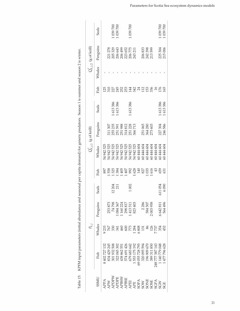
21
Parameters for Scotia Sea ecosystem dynamics models
Tab
le 1
5:
KPF
M in
put p
aram
eter
s (i
niti
al a
bund
ance
and
sea
sona
l per
cap
ita
dem
and
) for
gen
eric
pre
dat
ors.
Sea
son
1 is
sum
mer
and
sea
son
2 is
win
ter.
,kj
P* ,
,1k
jQ
(g o
f kri
ll)
* ,,2
kj
Q (g
of k
rill)
SSM
U
Fish
W
hale
s Pe
ngui
ns
Seal
s Fi
sh
Wha
les
Peng
uins
Se
als
Fish
W
hale
s Pe
ngui
ns
Seal
s
APP
A
8 40
2 72
7 13
2 9
233
897
54 9
42 5
25
125
-
A
PW
834
429
245
767
253
873
1
558
54 9
42 5
25
311
307
31
0 -
221
278
A
PDPW
30
1 93
2 50
8 33
0 74
798
12
204
1
325
54 9
42 5
25
255
235
1 61
3 38
6 22
7 -
205
329
1 03
9 70
0 A
PDPE
32
2 04
5 30
2 34
1 1
084
367
211
1 38
4 54
942
525
25
1 59
1 1
613
386
245
- 20
6 64
3 1
039
700
APB
SW
438
862
551
460
1 16
0 22
4
1 40
5 54
942
525
25
1 98
8
252
- 20
6 49
9
APB
SE
574
691
426
600
298
817
1
407
54 9
42 5
25
314
812
25
3 -
223
652
A
PEI
679
683
642
773
1 41
3 51
1 1
002
992
54 9
42 5
25
251
228
1 61
3 38
6 14
4 -
206
775
1 03
9 70
0 A
PE
1 55
3 17
5 19
2 1
284
823
403
1
628
54 9
42 5
25
366
713
34
2 -
243
211
SO
PA
69 0
55 7
28 7
95
6 80
8
14
0 60
444
604
24
-
SOW
32
0 09
5 59
4 13
1 2
286
82
7 60
444
604
25
1 06
5
112
- 20
6 83
3
SON
E
196
909
670
86
584
507
1
035
60 4
44 6
04
364
280
15
3 -
242
398
SO
SE
389
311
850
126
2 00
3 95
8
1 61
6 60
444
604
27
3 60
3
336
- 21
3 59
9
SGPA
24
8 77
7 38
7 14
3 7
737
43
60 4
44 6
04
16
-
SG
W
1 14
0 77
9 04
8 35
4 6
642
811
611
054
659
60 4
44 6
04
227
304
1 61
3 38
6 17
6 -
225
304
1 03
9 70
0 SG
E
1 47
7 79
6 62
8 45
2 56
4 49
6 6
090
631
60 4
44 6
04
246
586
1 61
3 38
6 16
5 -
215
006
1 03
9 70
0

Hill et al.
22
Liste des tableaux
Tableau 1: Défi nitions des paramètres du modèle KPFM mentionnés dans ce document.
Tableau 2: Nom des SSMU et des aires délimitées, surfaces et capture totale de krill (1988 à 2002). La zone de plateau se situe à une profondeur ≤500 m et la zone au large du plateau, à une profondeur >500 m. La surface des SSMU est calculée à partir du jeu de données de Smith et Sandwell (1997), celle des aires délimitées, à partir du jeu de données de la GEBCO (IOC et al., 2003), les données de capture de krill sont tirées de Hewitt et al. (2004a) et la biomasse de krill est le produit de la densité mentionnée dans Hewitt et al. (2004a) et de la surface mentionnée ici.
Tableau 3: Flux maximum instantanés de krill entre les secteurs modélisés indiqués sur la fi gure 1, pendant l’été. Les SSMU et les aires délimitées (BA pour boundary area) sont numérotés dans le tableau 2.
Tableau 4: Flux maximum instantanés de krill entre les secteurs modélisés, pendant l’hiver.
Tableau 5: Densité, poids corporel moyen et besoins en krill des deux principales espèces de myctophidés dépendantes du krill, échantillonnées dans les eaux de pentes proches de l’île du Roi George en 1996. Les données sont tirées de Pusch et al. (2004). Les estimations de la consommation sont basées sur une alimentation journalière de 10 heures (minimum) et de 24 heures (maximum).
Tableau 6: Biomasse estimée et besoins annuels en krill de sept espèces de poissons perciformes dans trois secteurs de la mer du Scotia pendant les campagnes d’évaluation menées au milieu des années 70 et dans la zone de plateau (≤500 m de profondeur) des SSMU non pélagiques de ces secteurs. Les données de biomasse et de consommation de krill sont adaptées (avec autorisation) de Kock (1985) (voir Note F7). Les données sur les surfaces proviennent du tableau 2.
Tableau 7: Autres hypothèses et paramètres utilisés pour calculer les paramètres génériques des poissons.
Table 16: Total krill demand (thousand tonnes), total biomass and krill consumption per unit biomass (Q/B) by taxonomic group and SSMU implied by the KPFM parameters in Table 15. Note that Q/B does not include consumption of prey other than krill and that adult consumption estimates for seals and penguins include dependent offspring. Fur seal mean body mass was assumed to be 35 kg for the purposes of estimating biomass. See also Notes F12 and S4.
SSMU Myctophid fish Perciform fish Whales Penguins Seals
APPA 3 889 3 647 507 APW 88 1 212 42 135 APDPW 94 306 18 34 32 APDPE 86 359 19 497 1 APBSW 110 506 25 532 APBSE 143 665 33 161 APEI 308 367 42 647 3 APE 37 2 492 71 502 SOPA 9 097 554 412 SOW 148 117 8 1 SONE 87 116 5 355 SOSE 15 614 8 976 SGPA 10 442 149 468 SGW 295 457 21 3007 1 621 SGE 393 540 27 261 16 Subtotal 25 234 12 102 1 706 7 108 1 673
Total 47 823 Biomass (thousand tonnes) 7 224 2 324 835 69 22 Annual Q/B 3.5 5.2 2.0 103.2 76.5

23
Parameters for Scotia Sea ecosystem dynamics models
Tableau 8: Projection démographique simple, montrant la survie prévue selon l'âge (à partir de l'âge 3) des otaries de Kerguelen et sex ratio des adultes d'âge supérieur à l'âge de la première reproduction, calculé à partir de là. Voir la note S2 pour davantage de détails.
Tableau 9: Paramètres de base des otaries de Kerguelen.
Tableau 10: Données de taille de la population de quatre colonies de manchots Adélie qui ne fi guraient pas dans SC-CAMLR (2002) et total par espèce des données fi gurant dans la version publiée du tableau.
Tableau 11: Biomasse (kg) par espèce de manchot reproducteur dans chaque SSMU. Les données sont tirées de SC-CAMLR (2002) et du tableau 10.
Tableau 12: Paramètres de chaque espèce de manchot.
Tableau 13: Paramètres de chaque espèce de baleine mysticète.
Tableau 14: Paramètres d'entrée du KPFM (paramètres du cycle biologique) pour les prédateurs génériques ( , ,k j sM est présumé constant quelle que soit la saison).
Tableau 15: Paramètres d’entrée du KPFM (abondance initiale et demande saisonnière par individu) pour les prédateurs génériques. La saison 1 correspond à l’été et la saison 2, à l’hiver.
Tableau 16: Demande totale de krill (milliers de tonnes), biomasse totale et consommation de krill par unité de biomasse (Q/B) par groupe taxonomique et par SSMU, sous-entendus par les paramètres du KPFM dans le tableau 15. Il est à noter que Q/B ne tient pas compte de la consommation de proies autres que le krill et que les estimations de la consommation des adultes chez les otaries et les manchots tiennent compte des jeunes dépendants. Le poids corporel moyen des otaries est fi xé à 35 kg pour les besoins de l’estimation de la biomasse. Voir également les notes F12 et S4.
Liste des fi gures
Figure 1: Régions de la mer du Scotia–péninsule antarctique, où sont indiqués les SSMU (dont les noms fi gurent dans le tableau 2), les aires délimitées et les sites mentionnés dans le texte.
Список таблиц
Табл. 1: Определения параметров модели КХПМ, полученных в данной работе.
Табл. 2: Названия SSMU и приграничных районов, районы и общий вылов криля (1988–2002 гг.). В районе шельфа глубина воды составляет ≤500 м, а вне шельфа >500 м. Площади SSMU рассчитаны по набору данных Смита и Сандвелла (Smith and Sandwell, 1997), приграничные районы рассчитаны по набору данных GEBCO (IOC et al., 2003), данные о вылове криля взяты из работы Hewitt et al. (2004a), а биомасса криля рассчитана на основе плотности, о которой говорится в работе Hewitt et al. (2004a), и приведенной здесь площади.
Табл. 3: Максимальная моментальная скорость переноса криля летом между модельными районами, показанными на рис. 1. SSMU приграничные районы (BA) пронумерованы как в табл. 2.
Табл. 4: Максимальная моментальная скорость переноса криля между модельными районами зимой.
Табл. 5: Плотность, средняя масса тела и потребности в криле для двух основных питающихся крилем миктофид, образцы которых были отобраны в водах на склоне у о-ва Кинг-Джордж в 1996 г. Данные из работы Pusch et al. (2004). Оценки потребления рассчитаны на основе периода кормления, равного 10 (минимум) и 24 (максимум) часам в сутки.
Табл. 6: Оценочная биомасса и годовая потребность в криле для семи видов окунеобразных рыб в трех районах моря Скотия во время съемок, проводившихся в середине 1970-х гг., а также в районе шельфа (на глубине ≤500 м) непелагических SSMU в этих районах. Данные о биомассе и потреблении криля приводятся с разрешения К.-Г. Кока (Kock, 1985) (см. Примечание F7). Данные о районах взяты из табл. 2.

Hill et al.
24
Табл. 7: Дополнительные допущения и параметры, использующиеся для расчета видовых параметров рыбы.
Табл. 8: Простой демографический прогноз, показывающий ожидаемую выживаемость по возрастам (с 3-летнего возраста) для южных морских котиков, и рассчитанное по нему соотношение самцов и самок старше возраста первого размножения. Более подробно см. Примечание S2.
Табл. 9: Основные параметры южных морских котиков.
Табл. 10: Данные о размере популяции четырех колоний пингвинов Адели, которые не были включены в отчет SC-CAMLR (2002 г.) плюс итоговые значения по видам для данных, включенных в опубликованный вариант таблицы.
Табл. 11: Биомасса (кг) по видам размножающихся пингвинов в каждой SSMU. Данные из отчета SC-CAMLR (2002) и табл. 10.
Табл. 12: Параметры отдельных видов пингвинов.
Табл. 13: Параметры отдельных видов усатых китов.
Табл. 14: Входные параметры модели КХПМ (параметры жизненного цикла) для основных хищников (при допущении о постоянном , ,k j sM во всех сезонах).
Табл. 15: Входные параметры модели КХПМ (исходная численность и сезонная потребность на одну особь) для основных хищников. Сезон 1 – лето, сезон 2 – зима.
Табл. 16: Общая потребность в криле (тыс. т), общая биомасса и потребление криля на единицу биомассы (Q/B) по таксономическим группам и SSMU, соответствующим параметрам КХПМ в табл. 15. Заметьте, что Q/B не включает потребления другой добычи, помимо криля, и что оценки потребления криля взрослыми тюленями и пингвинами включают выкармливаемых ими детенышей. В целях оценки биомассы средняя масса тела морского котика принимается за 35 кг. См. также примечания F12 и S4.
Список рисунков
Рис. 1: Район моря Скотия – Антарктического п-ова; показаны упомянутые в тексте SSMU (названия даются в табл. 2), приграничные районы и участки.
Lista de las tablas
Tabla 1: Defi niciones de los parámetros del modelo KPFM obtenidos de este trabajo.
Tabla 2: Nombre de las UOPE y áreas limítrofes, superfi cie y captura total de kril (1988 a 2002). El área de la plataforma comprende aguas de profundidad ≤500 m y el área fuera de la plataforma se refi ere a las aguas de profundidad >500 m. Las áreas de las UOPE se calcularon del conjunto de datos de Smith y Sandwell (1997), las áreas limítrofes se derivaron del conjunto de datos GEBCO (IOC et al., 2003), los datos de captura de kril se obtuvieron de Hewitt et al. (2004a) y la biomasa de kril es el producto entre el valor de la densidad informada en Hewitt et al. (2004a) y el área indicada en este trabajo.
Tabla 3: Tasas instantáneas máximas de transporte de kril entre las áreas del modelo mostradas en la fi gura 1 en el verano. Los números de las UOPE y de las áreas limítrofes (BAs) corresponden a los de la tabla 2.
Tabla 4: Tasas instantáneas máximas de transporte de kril entre las áreas del modelo en el invierno.
Tabla 5: Densidad, masa corporal promedio y demanda de kril de los dos principales mictófi dos depredadores de kril muestreados en las aguas del talud cerca de la Isla Rey Jorge en 1996. Datos de Pusch et al. (2004). Las estimaciones del consumo se basan en un mínimo de 10 horas y un máximo de 24 horas de alimentación al día.

25
Parameters for Scotia Sea ecosystem dynamics models
Tabla 6: Estimación de la biomasa y la demanda anual de kril de siete especies de peces perciformes en tres áreas del Mar de Escocia durante las campañas efectuadas a mediados de la década del 70, y el área de la plataforma (≤500 m de profundidad) de las UOPE no pelágicas en estas áreas. Los valores de biomasa y de consumo de kril han sido adaptados con el permiso de Kock (1985) (véase la nota F7). Los datos del área provienen de la tabla 2.
Tabla 7: Suposiciones y parámetros adicionales utilizados para calcular parámetros genéricos para los peces.
Tabla 8: Proyección demográfi ca simple, mostrando la supervivencia esperada por edad (desde edad 3) del lobo fi no antártico y la proporción de sexos de los ejemplares adultos que han pasado la edad de primera reproducción derivada de dicha proyección. Véase la nota S2 para más detalles.
Tabla 9: Parámetros básicos del lobo fi no antártico.
Tabla 10: Datos sobre el tamaño de la población de cuatro colonias de pingüinos adelia que no fueron incluidas en SC-CAMLR (2002), y totales por especie de los datos incluidos en la versión publicada de la tabla.
Tabla 11: Biomasa (kg) por especie de los pingüinos reproductores de cada UOPE. Datos de SC-CAMLR (2002) y de la tabla 10.
Tabla 12: Parámetros para especies individuales de pingüino.
Tabla 13: Parámetros para especies individuales de ballenas de barba.
Tabla 14: Parámetros de entrada del modelo KPFM (parámetros del ciclo de vida) de los depredadores genéricos (se supone que , ,k j sM permanece constante en todas las estaciones).
Tabla 15: Parámetros de entrada del modelo KPFM (abundancia inicial y demanda estacional per cápita) de los depredadores genéricos. La temporada 1 corresponde al verano y la temporada 2 al invierno.
Tabla 16: Demanda total de kril (miles de toneladas), biomasa total y consumo de kril por unidad de biomasa (Q/B) por grupo taxonómico y UOPE, derivados de los parámetros del KPFM de la tabla 15. Nótese que la razón Q/B no incluye el consumo de presas distintas de kril y que las estimaciones del consumo de pinnípedos y pingüinos adultos incluye a las crías dependientes. A los efectos de la estimación de la biomasa, se supuso una masa corporal promedio de los pinnípedos igual a 35 kg. Véanse además las notas F12 y S4.
Lista de las fi guras
Figura 1: Región del Mar de Escocia–Península Antártica, mostrando la ubicación de las UOPE (véase la tabla 2), las áreas limítrofes y los lugares mencionados en el texto.
