a comparison of the dynamical evolution of planetary systems || chaotic motions in the field of two...

CHAOTIC MOTIONS IN THE FIELD OF TWO FIXED BLACK HOLES

G. CONTOPOULOS and M. HARSOULAAcademy of Athens, Center for Astronomy

Soranou Efessiou 4, GR-11527, Athens, Greece

(Received: 6 September 2004; accepted: 29 November 2004)

Abstract. We study the chaotic motions in the field of two fixed black holes M1, M2 bycalculating (a) the asymptotic curves from the main unstable periodic orbits, (b) the asymp-

totic orbits, with particular emphasis on the homoclinic and heteroclinic orbits, and (c) thebasins of attraction of the two black holes. The orbits falling on M1 and M2 form fractal sets.The asymptotic curves consist of many arcs, separated by gaps. Every gap contains orbits

falling on a black hole. The sizes of various arcs decrease as the mass of M1 increases. Thebasins of attraction of the black holes M1, M2 consist of large compact regions and of thinfilaments. The relative area of the basin M2 tends to 100% as M1 fi 0, and it decreases as M1

increases. The total area of the basins is found analytically, while the relative area of the basin

M2 is given by an empirical formula. Further empirical formulae give the exponential decreaseof the number of asymptotic orbits that have not yet reached a black hole after n iterations.

Key words: Chaotic motion, two fixed black holes problem

1. Introduction

The problem of two fixed black holes refers to the motions of particles ofinfinitesimal mass (time-like geodesics) and photons (null geodesics) in thefield of two fixed centresM1 andM2. It is known that the classical problem oftwo fixed centres is integrable (Charlier, 1902; Deprit, 1960), while the rela-tivistic problem is chaotic (Contopoulos, 1990, 1991); namely the motions ofphotons are completely chaotic, while the motions of particles are chaotic toa large degree.

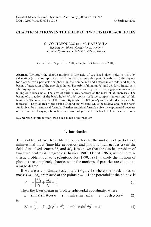
If we use a coordinate system x–z (Figure 1) where the black holes ofmasses M1, M2 are placed at the points z ¼ ±1 the potential at the point P is

V ¼ � M1

r1þM2

r2þ 1

� ð1Þ

Then the Lagrangian in prolate spheroidal coordinate, where

x ¼ sinhw sin h cosu; y ¼ sinhw sin h sinu; z ¼ coshw cos h ð2Þis

2L ¼ _t2

V 2� V2½Qð _w2 þ _h2Þ þ sinh2 w sin2 h _/2� ¼ d1 ð3Þ

Celestial Mechanics and Dynamical Astronomy (2005) 92:189–217DOI 10.1007/s10569-004-6878-8 � Springer 2005

(Chandrasekhar, 1989), where d1 ¼ 0 for photons and d1 ¼ 1 for particles,and

Q ¼ cosh2 w� cos2 h > 0 ð4Þwhile the dots represent derivatives with respect to an affine parameter. Fromthis Lagrangian we derive the energy E and the angular momentum Lz

integrals.From now on we consider orbits on a meridian plane and take Lz ¼ 0.In the case of particles the energy E is given by the equation

E2 ¼ Qð _w2 þ _h2Þ þ V�2: ð5ÞIf the energy is of the elliptic type we have 0<E<1 and the particles

cannot escape to infinity. Then there are some simple periodic orbits aroundone or the other black hole. These orbits intersect perpendicularly the z-axis.

In Figure 2 we give the characteristics of these periodic orbits, i.e., thevalues of z for various values of M1, assuming that M2 ¼ 1 and the energy Eis fixed (in Figure 2, E ¼ �0.5). We see that for 0<M1<M1max»1.3258 thereare two closed orbits of period 1 around M1 that we call a (inner) and a¢(outer) (in our previous papers we called both of them a¢). The orbits aand a¢ join at a maximum M1 and near this point the orbits a¢ are stable(Contopoulos, 1991).

Figure 1. The position of a particle P in the coordinate system x–z.

G. CONTOPOULOS AND M. HARSOULA190

For M1 > 0.9061 there are two orbits around M2 that we call b (inner)and b¢ (outer). These orbits join at a minimum M1 and near this point theorbits b¢ are stable. Orbits of types b and b¢ do not exist for values ofM1 closeto zero. However for larger values of the energy E there are orbits of this typefor smaller M1 and when Efi1 the orbits of types b, b¢ approach the limitM1 fi 0.

The orbits a, a¢, b, b¢ can be described in the opposite direction and thenthey are called �a, �a0, �b, and �b0. There is also a simple orbit like an arc ofhyperbola (orbit h) that is described in both directions.

The inner orbits a, �a or b, �b are very important, because any nonperiodicorbit crossing them inwards falls into the black holes M1, M2, respectively.

It is remarkable that in the classical case there are no simple periodicorbits around one black hole, i.e., satellite orbits closing after only onerotation around M1, or M2. This fact was established only relatively recently(Contopoulos, 1990).

One way to establish the existence of chaos in a dynamical system is bystudying the homoclinic and heteroclinic intersections of the asymptoticcurves from the unstable periodic orbits. On a surface of section (z, _z) forx ¼ 0 such intersections represent doubly asymptotic orbits. Another phe-nomenon related to chaos is the fractal structure of the basins of attraction ofthe orbits falling into the black holesM1 andM2. In this case many orbits fall

Figure 2. The characteristics of the periodic orbits a, a¢, h, b and b¢ for an energy E ¼ �0.5.

CHAOTIC MOTIONS 191

into the black holes and there are no Poincare surfaces of section. Thus, theproblem of two fixed black holes has certain properties of dissipative systems.

In the present paper we study the asymptotic curves of the periodic orbitsa, b, a¢, with emphasis on the homoclinic and heteroclinic orbits.

Our study extends the results of a previous paper of ours on the samesubject (Contopoulos and Harsoula, 2004).

In Section 2 we find the forms of the asymptotic curves and in Section 3 westudy the forms of the asymptotic orbits. The asymptotic orbits falling intothe black holes M1 and M2 form sets with a fractal structure. Then in Section4 we find the basins of attraction of the black holes M1 and M2 for variousvalues of M1 (with M2 ¼ 1) and in Section 5 we formulate our conclusions.

2. Asymptotic Curves

The asymptotic curves (z, _z) (for x ¼ 0, _x>0) of the periodic orbit O (oftype a) are shown in Figure 3 for M1 ¼ M2 ¼ 1. There are two unstableasymptotic curves U, UU and two stable asymptotic curves S, SS thatintersect with the U, UU curves at the homoclinic points H1, H2, and further

Figure 3. Parts of the asymptotic curves U, UU (unstable) and S, SS (stable) from the

unstable periodic orbit O”a for M1 ¼ M2 ¼ 1 and E ¼ �0.5. These unstable asymptotic curvesintersect the stable asymptotic curves at the homoclinic points H1, H2 and other points notmarked in this figure. The periodic orbits a¢, b and b¢ are also given.


points not shown in Figure 3. The curves S, SS are symmetric to the curvesU, UU with respect to the axis _z ¼ 0.

There is no symmetry with respect to the centre (0,0). The arc (1) of Uintersects its symmetric arc S above it, but the arc (3) of U is completelyabove the _z ¼ 0 axis and does not intersect its symmetric arc S below it.However, if we continue the asymptotic curve U of Figure 3 we find, inthe case M1 ¼ M2 ¼ 1, further arcs close to the arcs (1), (2), (3) thatintersect the symmetric arcs S at further homoclinic points. In particularthere are homoclinic points close to b and b¢, not marked in Figure 3.

We see that the asymptotic curves pass through the black holes M1 andM2 with velocities _z ¼ ±0.71. In the Appendix of paper I we have shownthat these values of _z are equal to _z ¼ ±E.

In Figures 4a, 5 and 6 we give one asymptotic curve U from the point Ofor M1 ¼ 1.1 (Figure 4a), M1 ¼ 1.2 (Figure 5) and M1 ¼ 1.24 (Figure 6),while M2 ¼ 1 in all cases. In Figure 4b we give both curves U and S forM1 ¼ 1.1.

The asymptotic curve U of Figure 4a starts at the point O upwards and tothe right. This curve consists of the 4th images of points starting close to O atdistances m · 10)8 along the asymptotic direction from O with m between 0and 20,000.

The asymptotic curve consists of several arcs reaching one or two blackholes, i.e., the points M�

1 ;Mþ1 ;M

�2 ;M

þ2 . The numbers in Figure 4a give the

values of m at the 4th iterations of the points m · 10)8.The first arc (1) starts at O and reaches the point M�

1 (point 207). Thenthe orbits with m ¼ 208–279 do not have a 4th intersection with thesurface of section x ¼ 0 ( _x > 0). Thus we have a gap in the initial con-ditions consisting of orbits that fall into a black hole before a 4th inter-section with the surface of section. Then follows the arc (2) starting at Mþ

1

with m ¼ 280 and terminating at M�1 with m ¼ 340. Further on we have a

gap between m ¼ 341 and m ¼ 412, an arc (3) from Mþ2 to the same point

Mþ2 with m ¼ 413 up to m ¼ 2054, and so on.The successive arcs start at a black hole, M1 or M2, and terminate at

the same, or the other black hole. Between any two arcs there are gaps,i.e., intervals of values of m without a 4th intersection.

In particular we notice that the arc (5) is a little below the arc (1).While the arc (1) is described clockwise, the arc (5) is described coun-terclockwise. It starts at M�

1 and returns again to M�1 . The point marked

2423 is on the arc (5) very close to the original point O.The various iterations of an initial point m · 10)8 are at distances

km · 10)8, k2m · 10)8, . . . , where k is the largest eigenvalue of theunstable orbit O.

CHAOTIC MOTIONS 193

Figure 4. (a) Part of the asymptotic curve U from O(”a), giving the 4th iterations of points

along the unstable asymptotic curve U from O at distances m · 10)8, where m varies fromm ¼ 0 up to m ¼ 20,000 for M1 ¼ 1.1, M2 ¼ 1, E ¼ �0.5. This curve consists of 11 successivearcs. The orbits a¢, b and b¢ are close but not exactly on the asymptotic curves from O. (b) the

arcs (1), (2), (3) and the corresponding arcs of the stable asymptotic curve S intersect at thehomoclinic points H1, H2, H3, H4.


In the case M1 ¼ 1.1 we have k ¼ 32.33. Thus a point marked m in Fig-ure 4a (4th iteration) is marked m3 ¼ km at its 3rd iteration, m5 ¼ m/k at its5th iteration, etc. Therefore the figure giving the 3rd, 5th etc. iterations is thesame as Figure 4a, and only the numbers denoting particular points aredifferent.

If we increase m beyond m ¼ 20,000 we find further arcs. But if the dis-tances m · 10)8 become larger than 2 · 10)4 we have better accuracy if westart closer to O, at distances m/k or m/k2, etc. and take the 5th, or 6th etc.iterations of the initial points.

In Figure 4b we see the first 3 arcs of the unstable asymptotic curve Ufrom O and the corresponding 3 arcs of the stable curve S. The arc (3) of Uintersects its symmetric arc S, in contrast with Figure 3 for M1 ¼ 1, and withsimilar figures with M1<1.

As we increase M1 the loops that we see in Figure 4a become shorter(Figures 5 and 6). For Example, the arc (3) in Figure 4a reaches the pointm ¼ 1160 and returns along a curve very close to the curve from m ¼ 413 tom ¼ 1180, reaching Mþ

2 at m ¼ 2054.In the case M1 ¼ 1.2 (Figure 5) this arc is much shorter, and in the case

M1 ¼ 1.24 the arc (3) does not exist at all. In this last case the arcs (2) and (4)of Figures 4a and 5 join and form a thin loop fromMþ

1 to the same pointMþ1

without reaching the point M2).

Figure 5. As in Figure 4 for M1 ¼ 1.2, M2 ¼ 1, E ¼ �0.5.

CHAOTIC MOTIONS 195

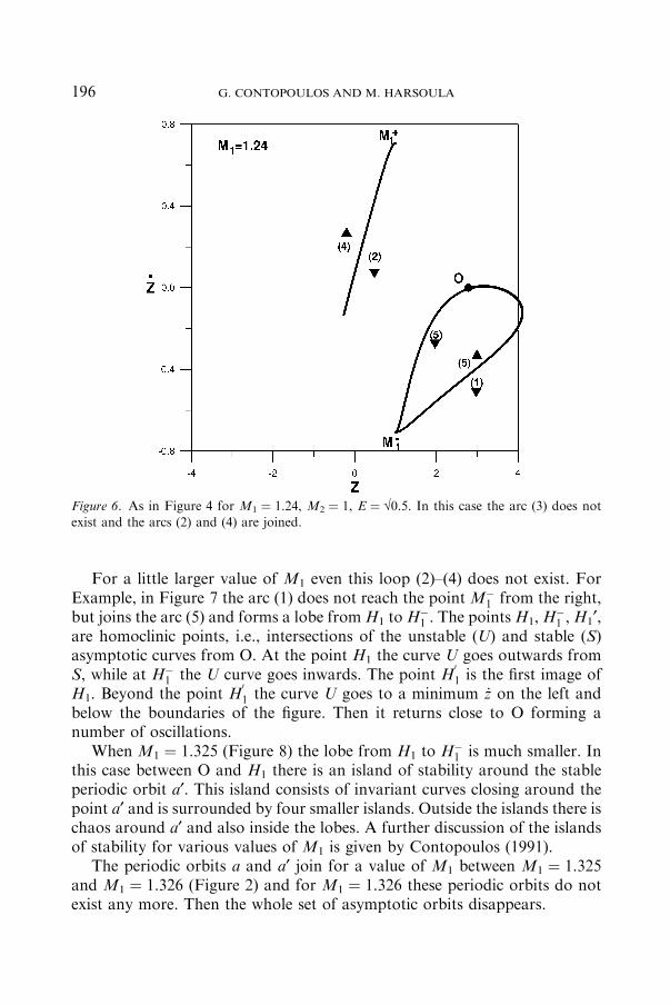
For a little larger value of M1 even this loop (2)–(4) does not exist. ForExample, in Figure 7 the arc (1) does not reach the point M�

1 from the right,but joins the arc (5) and forms a lobe fromH1 toH�

1 . The pointsH1,H�1 ,H1¢,

are homoclinic points, i.e., intersections of the unstable (U) and stable (S)asymptotic curves from O. At the point H1 the curve U goes outwards fromS, while at H�

1 the U curve goes inwards. The point H01 is the first image of

H1. Beyond the point H01 the curve U goes to a minimum _z on the left and

below the boundaries of the figure. Then it returns close to O forming anumber of oscillations.

When M1 ¼ 1.325 (Figure 8) the lobe from H1 to H�1 is much smaller. In

this case between O and H1 there is an island of stability around the stableperiodic orbit a¢. This island consists of invariant curves closing around thepoint a¢ and is surrounded by four smaller islands. Outside the islands there ischaos around a¢ and also inside the lobes. A further discussion of the islandsof stability for various values of M1 is given by Contopoulos (1991).

The periodic orbits a and a¢ join for a value of M1 between M1 ¼ 1.325and M1 ¼ 1.326 (Figure 2) and for M1 ¼ 1.326 these periodic orbits do notexist any more. Then the whole set of asymptotic orbits disappears.

Figure 6. As in Figure 4 for M1 ¼ 1.24, M2 ¼ 1, E ¼ �0.5. In this case the arc (3) does notexist and the arcs (2) and (4) are joined.


Figure 7. Parts of the asymptotic curves U and S from O for M1 ¼ 1.322, M2 ¼ 1, E ¼ �0.5close to O. The orbit a¢ is unstable.

Figure 8. As in Figure 7 for M1 ¼ 1.325, M2 ¼ 1, E ¼ �0.5. The periodic orbit a¢ is nowstable, and it is surrounded by closed invariant curves. Further out there are four smallislands. The scattered points belong to a single chaotic orbit outside the islands.

CHAOTIC MOTIONS 197

The orbits in the region of the gap m ¼ 208–279 are shown in Figure 9.These orbits start close to the periodic orbit a, above M1, with x ¼ 0 and_x > 0. All of them make three complete rotations clockwise around M1 andthen they deviate from each other. The orbits with a little smaller m thanm ¼ 208 have a 4th intersection with the z-axis a little above M1, and theyhave _z < 0. The orbit m ¼ 208 does not have a 4th intersection. In fact allthe orbits m ¼ 208–279 reach the black hole M1 from the left withoutintersecting the z-axis a 4th time. On the other hand the orbits with a littlelarger m than m ¼ 279 have again 4th intersections with the z-axis, and_z>0.

If we now take a surface of section (z, _z) with x ¼ )0.001 ( _x > 0), all theorbits of the gap have 4th intersections with this surface of section at pointsintermediate between M�

1 and Mþ1 (Figure 10). Thus the surface of section

x ¼ )0.001 does not indicate a gap in this case. Nevertheless these orbits donot have a 5th intersection with the surface (z, _z) (x ¼ )0.001, _x > 0) there-fore this surface is not a Poincare surface of section. Furthermore some gapsare not eliminated by using a surface of section x ¼ )0.001, because there areorbits reaching the black hole without a 4th intersection with any of thesurfaces x ¼ 0 or x ¼ )0.001.

Figure 9. Asymptotic orbits in the plane (x,z). The orbits with m between m ¼ 208 andm ¼ 279 do not have a 4th intersection with the z-axis before falling on M1. The orbitsm ¼ 207 and m ¼ 341 have a 4th intersection close to M1, the first above it and the second

below it.


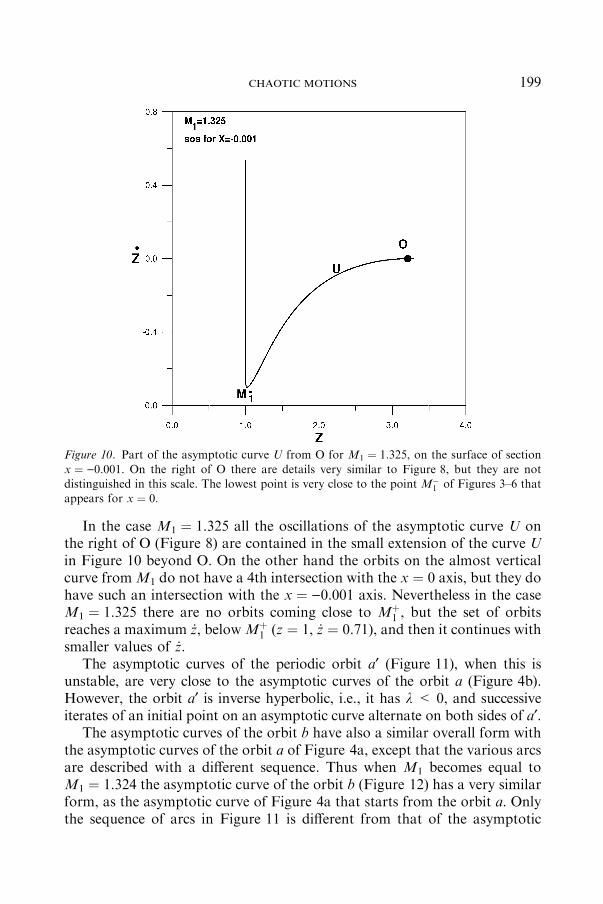
In the case M1 ¼ 1.325 all the oscillations of the asymptotic curve U onthe right of O (Figure 8) are contained in the small extension of the curve Uin Figure 10 beyond O. On the other hand the orbits on the almost verticalcurve fromM1 do not have a 4th intersection with the x ¼ 0 axis, but they dohave such an intersection with the x ¼ )0.001 axis. Nevertheless in the caseM1 ¼ 1.325 there are no orbits coming close to Mþ

1 , but the set of orbitsreaches a maximum _z, belowMþ

1 (z ¼ 1, _z ¼ 0.71), and then it continues withsmaller values of _z.

The asymptotic curves of the periodic orbit a¢ (Figure 11), when this isunstable, are very close to the asymptotic curves of the orbit a (Figure 4b).However, the orbit a¢ is inverse hyperbolic, i.e., it has k < 0, and successiveiterates of an initial point on an asymptotic curve alternate on both sides of a¢.

The asymptotic curves of the orbit b have also a similar overall form withthe asymptotic curves of the orbit a of Figure 4a, except that the various arcsare described with a different sequence. Thus when M1 becomes equal toM1 ¼ 1.324 the asymptotic curve of the orbit b (Figure 12) has a very similarform, as the asymptotic curve of Figure 4a that starts from the orbit a. Onlythe sequence of arcs in Figure 11 is different from that of the asymptotic

Figure 10. Part of the asymptotic curve U from O for M1 ¼ 1.325, on the surface of section

x ¼ )0.001. On the right of O there are details very similar to Figure 8, but they are notdistinguished in this scale. The lowest point is very close to the point M�

1 of Figures 3–6 thatappears for x ¼ 0.

CHAOTIC MOTIONS 199

curve from a. The asymptotic curves of the orbit b¢, when this is unstable, arealso very similar.

3. Asymptotic, Homoclinic and Heteroclinic Orbits

The asymptotic curves start at the unstable periodic point O along twoeigendirections, one unstable (U) and the other stable (S).

Further away these curves deviate from straight lines. An orbit starting ata point of an asymptotic curve is asymptotic to the periodic orbit O in thepast, for t ! �1 (in the case U), or in the future, for t ! þ1 (in the case S).

The successive iterates of an orbit in U are either all on the same side ofO (regular hyperbolic point), or alternatively on both sides of O (inversehyperbolic point). In the present case the orbits a and b are regular hyper-bolic, while the orbits a¢ and b¢ are inverse hyperbolic.

The intersections of the asymptotic curves U and S are homoclinic points,like the points H1, H2, of Figure 3 and the points H3, H4 of Figure 4b. Thecorresponding orbits are asymptotic to the same orbit both in the past(t ! �1) and in the future (t ! þ1).

Figure 11. Parts of the unstable and stable asymptotic curves U and S from the periodic orbit

a¢ for M1 ¼ 1.1.


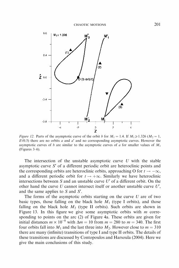
The intersection of the unstable asymptotic curve U with the stableasymptotic curve S¢ of a different periodic orbit are heteroclinic points andthe corresponding orbits are heteroclinic orbits, approaching O for t ! �1,and a different periodic orbit for t ! þ1. Similarly we have heteroclinicintersections between S and an unstable curve U¢ of a different orbit. On theother hand the curve U cannot intersect itself or another unstable curve U¢,and the same applies to S and S¢.

The forms of the asymptotic orbits starting on the curve U are of twobasic types, those falling on the black hole M1 (type I orbits), and thosefalling on the black hole M2 (type II orbits). Such orbits are shown inFigure 13. In this figure we give some asymptotic orbits with m corre-sponding to points on the arc (2) of Figure 4a. These orbits are given forinitial distances m · 10)8 with Dm ¼ 10 from m ¼ 280 to m ¼ 340. The firstfour orbits fall into M1 and the last three into M2. However close to m ¼ 310there are many (infinite) transitions of type I and type II orbits. The details ofthese transitions are discussed by Contopoulos and Harsoula (2004). Here wegive the main conclusions of this study.

Figure 12. Parts of the asymptotic curve of the orbit b for M1 ¼ 1.4. If M1P1.326 (M2 ¼ 1,E�0.5) there are no orbits a and a¢ and no corresponding asymptotic curves. However the

asymptotic curves of b are similar to the asymptotic curves of a for smaller values of M1

(Figures 3–6).

CHAOTIC MOTIONS 201

1. The sets of types I and II are fractal consisting of infinite subsets. Everysubset is limited by homoclinic or heteroclinic orbits.

2. Near every homoclinic and heteroclinic orbit there are infinite furtherhomoclinic and heteroclinic orbits and infinite subsets of type I and II orbits.

3. All the orbits of the arc (2) with m < m*»307.643390 are of type I (theyfall intoM1) and all the orbits of this arc with m > m**»314.384627 are oftype II (they fall into M2).

In particular the orbit with m ¼ m* (Figure 14) is a heteroclinic orbitjoining the orbit a (for t ! �1) to the orbit �a (for t ! þ1), i.e., the sameorbit described in the opposite direction (for this reason the orbit �a isconsidered as different form a). The orbit m ¼ m* after infinite rotationsclockwise reaches a minimum x at a point with _z ¼ 0, therefore it retraces itspath in the opposite direction, reaching the orbit �a after infinite rotationscounterclockwise.

If we decrease m all the orbits fall into M1, as m decreases until m ¼ 75.The interval 75 < m < m* contains not only orbits of the upper part of thearc (2) of Figure 4a but also all the orbits of the gap between the arcs (1) and

Figure 13. Some asymptotic orbits corresponding to points m on the arc (2) of Figure 4. These

orbits fall either on M1 (if m O 300), or on M2 (if m P 320). But close to m ¼ 310 there areinfinite sets of orbits falling into M1 and M2.


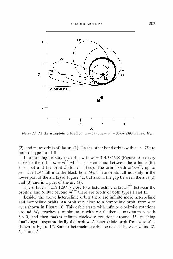
(2), and many orbits of the arc (1). On the other hand orbits with m < 75 areboth of type I and II.

In an analogous way the orbit with m ¼ 314.384628 (Figure 15) is veryclose to the orbit m ¼ m** which is heteroclinic between the orbit a (fort ! �1) and the orbit �b (for t ! þ1). The orbits with m>m**, up tom ¼ 559.1297 fall into the black hole M2. These orbits fall not only in thelower part of the arc (2) of Figure 4a, but also in the gap between the arcs (2)and (3) and in a part of the arc (3).

The orbit m ¼ 559.1297 is close to a heteroclinic orbit m*** between theorbits a and b. But beyond m*** there are orbits of both types I and II.

Besides the above heteroclinic orbits there are infinite more heteroclinicand homoclinic orbits. An orbit very close to a homoclinic orbit, from a toa, is shown in Figure 16. This orbit starts with infinite clockwise rotationsaround M1, reaches a minimum x with _z < 0, then a maximum x with_z > 0, and then makes infinite clockwise rotations around M1 reachingfinally again asymptotically the orbit a. A heteroclinic orbit from a to �a0 isshown in Figure 17. Similar heteroclinic orbits exist also between a and �a0,�b, b0 and �b0.

Figure 14. All the asymptotic orbits from m ¼ 75 to m ¼ m* ¼ 307.643390 fall into M1.

CHAOTIC MOTIONS 203

Further details about the homoclinic and heteroclinic orbits and thefractal structure of the sets of orbits I and II are given by Contopoulos andHarsoula (2004).

4. Basins of Attraction

The basins of attraction of two and three black holes and their fractalstructure were considered by Dettmann et al. (1994, 1995). In the presentpaper we consider the basins of attraction for various values of the mass M1

and their relations with the asymptotic manifolds discussed in the previoussections. If we calculate all orbits with M1 ¼ 1.1, M2 ¼ 1 and E ¼ �0.5 andinitial conditions on the surface of section (z, _z) (with x ¼ 0 and _x>0)we find(Figure 18) large sets falling directly intoM1 andM2 without any intersectionwith the surface of section (black and gray respectively) and smaller sets thatfall into M1, or M2, after 1, or 2, or more intersections. These sets consist oflarge compact regions and of thin filaments. A few filaments can be seen inFigure 18.

These filaments form fractal sets. They correspond to the sets Dm of valuesof m along the unstable asymptotic curve from the orbit a that are terminated

Figure 15. All the asymptotic orbits from m ¼ m** ¼ 314.384627. . . to m*** ¼ 559.1297. . . fallinto M2.


by homoclinic or heteroclinic orbits and fall into M1, or M2. Figures 18–21are calculated by taking initial conditions on the surface of section at a gridof points with sizes Dz ¼ 10)2 and d _z ¼ 0:8 · 10)2. If we compare Figure 18with Figure 4a we see two filaments passing through the central part of thearc (2), namely in the region between the first heteroclinic point m ¼ m* andthe last heteroclinic point m ¼ m** in this region. More detailed figures of thecentral part of Figure 18 show many more filaments that are limited by thehomoclinic and heteroclinic points along the arc (2).

The upper part of the arc (2) of Figure 4a, i.e., with m < m*, does notcontain any homoclinic or heteroclinic orbits. These orbits are in the blackregion of Figure 18, therefore they escape immediately into the black hole M1.

In fact the points on the arc (2) are the 4th iterates of points close to O alongthe asymptotic curve U at distances m · 10)8, and the starting orbits in thispart of the arc (2) do not have a 5th intersection with the surface of section, butfall into M1 after the 4th intersection. In the same way at the points of thelower part of the arc (2), with m>m**, start orbits that fall directly into theblack hole M2 without a 5th intersection with the surface of section.

Two more regions with many (infinite) filaments of orbits escaping toM1 and M2 form loops in the upper right part and in the lower left part

Figure 16. A homoclinic orbit starting asymptotically close to the periodic orbit a (ast ! �1) and reaching again asymptotically the same orbit a (as t ! 1).

CHAOTIC MOTIONS 205

of Figure 18. These loops surround a compact gray region on the upperright (type II orbits) and a compact black region on the lower left (type Iorbits). The loops contain filaments with orbits falling into either M1 orM2, after one or more iterations. The limits of the filaments falling intoM1 and M2 pass through the homoclinic and heteroclinic points along theasymptotic curves U and S of Figure 4b.

As M1 increases the area covered by orbits on the surface of sectionincreases (see Appendix A), while the points M�

1 , Mþ1 , M

�2 , Mþ

2 , remainthe same. Examples are shown in Figures 19 and 20. We see that, as M1

increases the black regions increase, therefore more orbits fall into M1

than into M2. In particular the gray upper right region becomes smallerand for M1 P 1.326 it does not reach the axis _z ¼ 0. This corresponds tothe fact that for M1 P 1.326 the periodic orbits a, a¢ and their asymptoticcurves with the corresponding homoclinic and heteroclinic intersectionsdisappear.

On the other hand the black region on the lower left side becomeslarger as M1 increases. This region intersects the _z ¼ 0 axis and justoutside it are the periodic points b and b¢, with their asymptotic curvesand their homoclinic and heteroclinic intersections.

Figure 17. A heteroclinic orbit between a and a¢. This orbit starts asymptotically from theorbit a for t ! �1 and terminates asymptotically on the orbit a¢ for t ! 1.


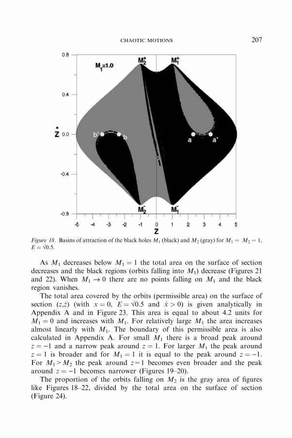
As M1 decreases below M1 ¼ 1 the total area on the surface of sectiondecreases and the black regions (orbits falling into M1) decrease (Figures 21and 22). When M1 fi 0 there are no points falling on M1 and the blackregion vanishes.

The total area covered by the orbits (permissible area) on the surface ofsection (z, _z) (with x ¼ 0, E ¼ �0.5 and _x > 0) is given analytically inAppendix A and in Figure 23. This area is equal to about 4.2 units forM1 ¼ 0 and increases with M1. For relatively large M1 the area increasesalmost linearly with M1. The boundary of this permissible area is alsocalculated in Appendix A. For small M1 there is a broad peak aroundz ¼ )1 and a narrow peak around z ¼ 1. For larger M1 the peak aroundz ¼ 1 is broader and for M1 ¼ 1 it is equal to the peak around z ¼ )1.For M1>M2 the peak around z=1 becomes even broader and the peakaround z ¼ )1 becomes narrower (Figures 19–20).

The proportion of the orbits falling on M2 is the gray area of figureslike Figures 18–22, divided by the total area on the surface of section(Figure 24).

Figure 18. Basins of attraction of the black holesM1 (black) andM2 (gray) forM1 ¼ M2 ¼ 1,E ¼ �0.5.

CHAOTIC MOTIONS 207

If M1 fi 0 this proportion goes to 1. However if M1 is exactly equal tozero only a set of orbits of measure zero fall into M2.

For small M1 most of the permissible area is filled with orbits falling intoM2 (Figures 21 and 22). In particular the black region close to M�

2 (thatcontains orbits falling into M1) is very small, and the black region on theright of the line M�

1 Mþ2 is thinner than in the case M1 ¼ 1 (compare Figures

21 and 18). As M1 tends to zero both these black regions tend to disappear(Figure 22).

On the other hand as M1 increases the black regions increase(Figures 18–20), while the gray regions become relatively smaller.

The total per cent proportion P of the gray regions as a function ofM1 canbe given approximately by the formula (Figure 24)

logP ¼ 1:9656� 0:2546M1 ð6ÞMost orbits of the black and gray regions fall immediately into the

black holes M1 and M2 respectively, i.e., without any intersection with thesurface of section (z, _z) (x ¼ 0, _x > 0). However a small proportion of



orbits have one, two, or more intersections with the surface of section (z, _z)before falling into M1 or M2. Finally a very small proportion of orbits aretrapped around stable periodic orbits (when such orbits exist) and never fallinto M1 or M2. An example of such trapped orbits, that form islands ofstability and never fall into M1 or M2, is shown in Figure 8. Such orbitshave been discussed by Contopoulos (1991). These orbits may define closedinvariant curves around stable periodic orbits, or be chaotic, but withoutever reaching either black hole.

In order to study further how various orbits fall into the black holes wehave calculated the proportion of orbits, along the asymptotic curve fromO(”a) that have n intersections with the surface of section before fallinginto one of the black holes, where n ¼ 1,2,3 etc. In Figure 25 we give thelogarithm of the proportion of orbits remaining after n intersections as afunction of n, for various values of M1. We find approximately

Figure 20. As in Figure 18 for M1 ¼ 2, M2 ¼ 1, E ¼ �0.5. In this case the orbits a, a¢ donot exist. Nevertheless, the basins of attraction of M1, M2 are similar to those of Figures 18

and 19.

CHAOTIC MOTIONS 209

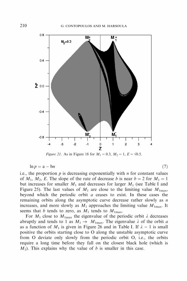
ln p ¼ a� bn ð7Þi.e., the proportion p is decreasing exponentially with n for constant valuesof M1, M2, E. The slope of the rate of decrease b is near b ¼ 2 for M1 ¼ 1but increases for smaller M1 and decreases for larger M1 (see Table I andFigure 25). The last values of M1 are close to the limiting value M1max,beyond which the periodic orbit a ceases to exist. In these cases theremaining orbits along the asymptotic curve decrease rather slowly as nincreases, and more slowly as M1 approaches the limiting value M1max. Itseems that b tends to zero, as M1 tends to M1max.

For M1 close to M1max the eigenvalue of the periodic orbit k decreasesabruptly and tends to 1 as M1 fi M1max. The eigenvalue k of the orbit aas a function of M1 is given in Figure 26 and in Table I. If k ) 1 is smallpositive the orbits starting close to O along the unstable asymptotic curvefrom O deviate only slowly from the periodic orbit O, i.e., the orbitsrequire a long time before they fall on the closest black hole (which isM1). This explains why the value of b is smaller in this case.



5. Conclusions

1. In the case of two fixed black holes most of the chaotic orbits (but not all)fall into the black holes M1 (orbits of type I), or M2 (orbits of type II). Thesetwo sets of orbits are fractal, consisting of infinite subsets limited byhomoclinic and heteroclinic orbits.2. The homoclinic and heteroclinic points on a surface of section (z, _z) (withx ¼ 0, _x > 0) are intersections of the asymptotic curves of the main unstableperiodic orbits a, a¢, �a, �a0 (around M1), h (hyperbolic-like) and b, b¢, �b, �b0

(around M2). These asymptotic curves pass through the black holes M1

(z ¼ 1) and M2 (z ¼ )1) with velocities _z ¼ �E (points M�1 ;M

�2 ) or _z ¼ þE

(points Mþ1 ;M

þ2 ).

3. The asymptotic curves consist of several separate arcs, like (1), (2), (3), . . .that terminate at one or two black holes. Between two successive arcs thereare gaps containing orbits that fall into the black holes M1 or M2.4. If we increase M1, keeping M2 ¼ 1 and E ¼ �0.5, we find that various arcsbecome shorter, and may not reach one, or the other black hole.


CHAOTIC MOTIONS 211

Figure 23. The total area on the surface of section (z, _z) (with x ¼ 0, E ¼ �0.5 and _x > 0) as a

function of M1.

Figure 24. The logarithm of the percent proportion of the area of orbits falling on the blackhole M2.


5. If we use a slightly different surface of section (x ¼ )0.001) most (but notall) of the gaps disappear. Nevertheless, the orbits falling into the black holesdo not have higher order intersections with the surfaces of section, thereforethese surfaces are not Poincare type surfaces of section.6. As M1 reaches a maximum value M1max (»1.3255 in the present case) theorbits a and a¢ join and for larger M1 they disappear. For M1 slightly smallerthen M1max the orbit a¢ is stable, and is surrounded by islands of stability.7. The asymptotic curves of the orbits a¢, b, b¢ are very similar to those oforbit a.8. The basins of attraction of the two black holes consist of large compactregions and of thin filaments forming fractal sets. The set of permissibleorbits can be calculated analytically. It increases with M1, almost linearly forlarge values of M1.9. The relative sizes of the set of orbits falling intoM1 increases, and the set oforbits falling into M2 decreases as M1 increases. If M1 decreases and tends tozero, this set also decreases and tends to zero. The relative size of the set M2

as a function of M1 decreases almost exponentially.

Figure 25. The logarithm of the proportion p of orbits starting along the asymptotic curvefrom O that remain after n intersections with the surface of section (before falling into a black

hole). The curves ln p versus n for various values of M1 are approximately straight lines withslopes b marked (Table I).

CHAOTIC MOTIONS 213

10. Finally we calculate the proportion p of orbits along an asymptotic curvethat remains after n ¼ 1,2,3, . . . intersections with the surface of section,before the orbits fall on a black hole. For fixed M1, M2 and E this proportiondecreases exponentially with n (ln p ¼ a ) bn). The slope b decreases as M1

increases, and tends to zero as M1 tends to M1max. This is explained by thefact that the eigenvalue k of the orbit a decreases and tends to 1 as M1 fiM1max.

Acknowledgements

This Research was supported by The Research Committee of the Academy ofAthens (Program 200/557). We thank Dr. Efthymiopoulos for helping us incalculating Figure 23.

TABLE I

M1 0.5 1.0 1.3 1.31 1.32 1.322 1.325

b 3.25 2.08 1.86 1.49 0.90 0.34 0.13k 44.98 36.43 13.71 11.23 7.58 6.48 3.79

Figure 26. The eigenvalue k of the orbits O(”a) as a function of M1.


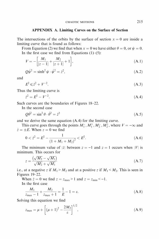
APPENDIX A. Limiting Curves on the Surface of Section

The intersections of the orbits by the surface of section x ¼ 0 are inside alimiting curve that is found as follows:

From Equation (2) we find that when x ¼ 0 we have either h ¼ 0, or w ¼ 0.In the first case we find from Equations (1)–(5):

V ¼ � M1

jz� 1j þM2

jzþ 1j þ 1

� ; ðA:1Þ

Q _w2 ¼ sinh2 w � _w2 ¼ _z2; ðA:2Þand

E2O _z2 þ V�2: ðA:3ÞThus the limiting curve is

_z2 ¼ E2 � V�2: ðA:4ÞSuch curves are the boundaries of Figures 18–22.

In the second case

Q _h2 ¼ sin2 h � _h2 ¼ _z2 ðA:5Þand we derive the same equation (A.4) for the limiting curve.

This curve goes through the points M�1 ;M

þ1 ;M

�2 ;M

þ2 , where V ¼ )1 and

_z ¼ �E. When z ¼ 0 we find

0 < _z2 ¼ E2 � 1

ð1þM1 þM2Þ2< E2: ðA:6Þ

The minimum value of | _z| between z ¼ )1 and z ¼ 1 occurs when |V| isminimum. This occurs for

z ¼ffiffiffiffiffiffiffiM2

p � ffiffiffiffiffiffiffiM1

p� �ffiffiffiffiffiffiffiM2

p þ ffiffiffiffiffiffiffiM1

p ðA:7Þ

i.e., at a negative z if M1>M2 and at a positive z if M1<M2. This is seen inFigures 19–22.

When _z ¼ 0 we find z ¼ zmax>1 and z ¼ zmin<)1.In the first case

M1

zmax � 1þ M2

zmax þ 1¼ 1

E� 1 ¼ e: ðA:8Þ

Solving this equation we find

zmax ¼ lþ ðlþ 1Þ2 � 2M2

e

� 1=2; ðA:9Þ

CHAOTIC MOTIONS 215

where

l ¼ M1 þM2

2e: ðA:10Þ

In the second case

M1

1� zmin� M2

1þ zmin¼ e: ðA:11Þ

Solving this equation we find

zmin ¼ �l� ðl� 1Þ2 þ 2M2

e

� 1=2: ðA:12Þ

If M1>M2 we have zmax>|zmin| and if M1<M2 we have |zmin|>zmax.In the particular case of Figure 16 where M1 ¼ M2 ¼ 1, E ¼ �0.5 ¼ 1/�2

we have e ¼ �2)1 ¼ 0.414, l ¼ 1/e ¼ �2+1 ¼ 2.414 and zmax ¼ |zmin|¼ l+(l2+1)1/2 ¼ 5.027.If M1fi0 we have the same e, but l ¼ 1/2e ¼ E=2ð1� EÞ ¼1.207 and

zmax ¼ 2l)1 ¼ 2E� 1=1� E ¼1.414, while zmin ¼ )2l)1 ¼ �1=1� E ¼)3.414. On the other hand if M1 is large we have l » M1/2e andzmax » 2l » M1/e while zmin » )2l » )zmax.

The area of initial conditions on the surface of section (z, _z) is

A ¼ 2

Z zmin

zmax

_z dz; ðA:13Þ

where _z is given from Equation (A.4), while V has the following expres-sions

If z > 1; V ¼ V1 ¼ � M1

z� 1þ M2

zþ 1þ 1

� ; ðA:14Þ

If 1 > z > �1; V ¼ V2 ¼ � M1

1� zþ M2

1þ zþ 1

� ; ðA:15Þ

and if � 1 > z; V ¼ V3 ¼ � M1

1� z� M2

1þ zþ 1

� : ðA:16Þ

Then using the package of Mathematica we find the area as a function ofM1, M2 and e. The values of A as a function of M1 for M2 ¼ 1 and e ¼ �2)1are given in Figure 23.

The boundary of this area can also be calculated from Equation (A.4). ForM1 ¼ 0 this boundary is symmetric around an axis z ¼ )1. When M1 is smallthere is a narrow peak around z ¼ 1 reaching _z ¼ E ¼ p

0:5 (Figure 22),while for larger M1 this peak is broader (Figures 18–21).


References

Chandrasekhar, S.: 1989, Proc. Roy. Soc. London A 421, 227.Charlier, C. L.:1902, ‘‘Die Mechanik des Himmels’’, von Veit, Leipsig.

Contopoulos, G.: 1990, Proc. Roy. Soc. London A 431, 183.Contopoulos, G.: 1991, Proc. Roy. Soc. London A 435, 551.Contopoulos, G. and Harsoula, M.: 2004, J. Math. Phys. 45, 4932.

Deprit, A.: 1960, Mathematiques du XXeme sciecle, Univ. Louvain 1, 45.Dettman, C. P., Frankel, N. E. and Cornish, N. J.: 1994, Phys. Rev. D 50, R618.Dettman, C. P., Frankel, N. E. and Cornish, N. J.: 1995, Fractals 3, 161.

CHAOTIC MOTIONS 217

a comparison of the dynamical evolution of planetary systems || chaotic motions in the field of two...

Documents