a comparison of the current crisis with the great ... · great depression as regards their depth...
TRANSCRIPT

Karl Aiginger
A comparison of the Current Crisis with the
Great Depression as regards their depth and
the policy responses
Abstract:
This paper compares the Great Depression and the Current Crisis. It builds on the existing
knowledge, what problems have lead to the Current Crisis, and to which extent the problems
were similar and different from that in the Great Depression. The focus of this paper, however,
is to report stylized facts about the depth of the crises (the extent to which GDP,
manufacturing production, employment, and stock prices dropped) and how economic
policy reacted during the Great Depression and today. We also investigate to what extent
different regions were affected depending on the crisis and whether the synchronization with
which the Current Crisis spread was larger this time due to globalization. Finally, the
probability is assessed that the fall in production has leveled off in 2009 and how economic
policy should react in this phase (specifically since unemployment will stay very high (or will
further increase).
JEL No: E20, E30, E32, E44, E60, G18, G28
Keywords: financial crisis, business cycle, stabilisation policy, resilience
Karl Aiginger
Austrian Institute of Economic Research WIFO
P.O. Box 91, A-1103 Vienna, Austria
Tel: +43 1 798 26 01-210, Fax: +43 1 798 26 01-306
[email protected], www.wifo.ac.at/Karl.Aiginger

– 2 –
Karl Aiginger
A comparison of the Current Crisis with the
Great Depression as regards their depth and
the policy responses
1. Introduction and outline
The aim of this paper is to compare the Current Crisis with the economic crisis of the nineteen
thirties (often referred to as the Great Depression, see Bernanke, 2004). The causes of the crisis
are not in the centre of this paper (for this see Aiginger, 2009, Bernanke, 2004, Cooper (2008),
Friedmann Schwartz, 1963, Krugman (2009), Eichengreen O’Rourke, 2009, Galbraith, 1954,
Schulmeister, 2009, Butschek, 1985, Sinn, 2009), but have to be kept in mind, therefore we
present also data on the build-up phase and we summarize our assessment in the appendix.
The main focus is the depth of each crisis and the response of economic policy. It may be too
soon in the Current Crisis to attempt such a comparison (or even premature). There are signs
that in production and world trade the Current Crisis has leveled off, and in most countries the
stock markets have definitely recovered between February 2009 and September 2009.
However, there is no guarantee that the world economy will not be hit by a second wave of
problems and at the least there will be echo effects and periods where stock prices might
decline. As far as unemployment, and probably also as far as insolvencies, are concerned
the “Current Crisis” is not over at all. Private sector production is not rising in any industrialized
country with sufficient speed or stability that the end of the crisis can be heralded. Even more
premature is the analysis of the policy response, which we know about only for the first year or
the first two years of the Current Crisis. We do not know the policy response in 2010 and later,
especially if the crisis should prove to be broader and longer than indicators currently suggest
in autumn 2009. Of course we do not know how fiscal and governmental policy will actually
react in the “exit phase”, when growth has started but employment as well as fiscal deficits
approach the 10% level in many countries. And the negative social and economic
consequences of the crisis will, in any event, be long lasting.
The author wishes to thank Gerhard Allgäuer, Felix Butschek, Burghard Feuerstein, Franz Hahn, Jürgen Janger,
Helmut Kramer, Karl Pichelmann, Hans Pitlik, Sonja Schneeweiss, Margit Schratzenstaller, Helene Schuberth, Stephan
Schulmeister, Hans Seidel, Egon Smeral, Hannes Stattmann, Peter Szopo, Gunther Tichy, Thomas Url and Ewald
Walterskirchen for their valuable contributions. However, any opinions expressed in the article remain the sole
responsibility of the author and do not always reflect the opinions of the critics. I am grateful to Dagmar Guttmann
and Christa Magerl for their research assistance and the WIFO team of Research Assistances for providing data in the
WIFO Long-term Database (Silvia Haas, Sandra Schneeweiß, Andrea Sutrich and Roswitha Übl).
– 3 –
2. Stylized Economic Facts
2.1 Comparing the depth of the crises as reflected by real GDP
Comparing the crisis in the nineteen thirties (referred to as the “Great Depression”) with the
recent one (referred to as the “Current Crisis”), reveals three stylized facts:
in both crises the build-up period was a period of high growth;
growth was much more stable and less cyclical in the build–up period to the Current
Crisis (in spite of the dot.com crisis which, with hindsight, was actually merely a growth
recession), whilst in the USA in the 1920’s there had been a recession and a variety of
post-war troubles in Europe;
the fall in GDP in the Great Depression dwarfed the decline in the Current Crisis; in most
industrialized countries it is likely that there will only be one year with declining GDP (2009)
and the decline of world GDP in this year will prove to be smaller than the increase in the
previous year and maybe also that of the following year.
The build-up phase
Even using annual GDP data we can still see the pattern of and the instability of growth in the
build-up to the Great Depression. World economic output increased by 45% between 1921
and 1929 (4.7% p.a.; see table 1)1. The development was bumpy with three absolute declines
including a rather severe recession in the early twenties. The turmoil came as a consequence
of World War I (WW I), which was felt even in the US. In European countries intermediate falls
in GDP were more pronounced, production was still not higher in many countries than pre-
war level, reparation payment were done, hyperinflation occurred etc. (figure 1).
By contrast this time world output increased very steadily between 1990 and 2008. Growth
amounted to 84% (3.5% p.a.) with no absolute decline in world GDP, in the USA and most
European countries. The only exception among developed countries was Japan, which
experienced a prolonged crisis between 1992 and 2003 (the “lost decade”). This was
following a period of stronger growth where Japan successfully caught up with the rest of the
world between 1950 and 1990. Between 2003 and 2007 growth in Japan was much less in
Japan than in the USA or in Europe.
US literature has labeled the period between1990 and 2000 (or 2008) as the period of “Great
Moderation” since there was high growth without severe inflation. Even the dot.com crisis is
difficult to find in the US GDP figures.2
1 If we compare the peak of 1929 with 1912 the growth of GDP had been 39%. We use data in constant dollar/PPP,
Geary-Khamis.
2 GDP increased by 0.8% and 1.6% respectively in the USA in the two years following the dot.com boom which may
actually be called a growth recession rather than a crisis.

– 4 –
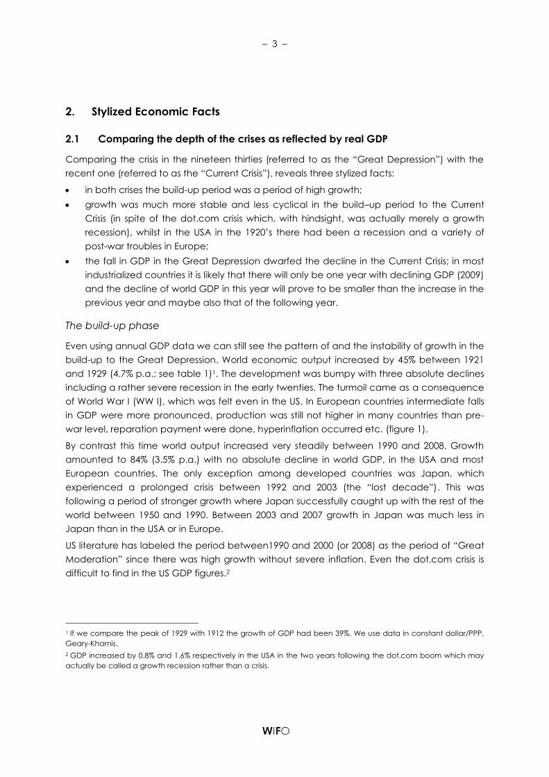
The decline and patterns across countries in the Great Depression
The decline of world GDP between 1929 and 1932 reached between 15% and 27% of its
previous peak (using annual data) in those countries hit most severely by the crisis (the USA,
Germany, France and Austria). It was 10% for the world (in PPP) or in the unweighted average
of the countries in Table 1. The decline in production lasted three years. The previous peak
was reached again in 1935 (after six years).
The pattern of world output was shaped by the USA (which at the time of the Great
Depression supplied 24% of world output (according to PPP values; it may have been 30% on
exchange rates). US growth in the build-up phase was approximately the same as the growth
in world GDP if we compare 1921 to 1929 (and stronger if we start in 1912). Higher growth in
the pre-crisis period was experienced in France, Sweden, and Spain, all following severe
losses in WWI. The decline between 1929 and 1932 was definitely more severe in the USA
(27%), followed by Austria (-20%), then Germany (-16%) and then France (-15%). The
recession was really mild (less or equal to 6% in three years cumulated) in Spain, Finland,
Sweden and the United Kingdom. GDP continued to increase in some countries (Denmark
and Norway). In summary world output declined rather dramatically between 1929 and 1932,
namely 10%, and this was the case even though in some countries the recession was mild
according to traditional pre WWII standards.
If we go further into details, the causes for the crisis and the starting level look rather different.
In the US the crisis started with stock market crashes, after a period of high optimism,
speculation and financial innovations (installment, credits etc.). Monetary policy had just tried
to dampen speculation in the phase of an already faltering business cycle. In Germany and
Austria past growth had been high, but hyperinflation at the start of the twenties were still in
mind and production was low as compared to pre-war level. Further repercussions from WWI
existed (reparation payments, restrictions as to trade policy); the political system was rather
unstable. It looks in some way as there would have been very different economic situations at
the start, which were “coordinated” by stock market developments, then by drops in export
markets and finally by bank runs and failures. Nevertheless the coefficient of variation in
table 1 shows much higher dispersion in the loss of output for the Great Depression.

– 5 –
Table 1: Comparison of two crises: decline of real GDP
1929/1921 1929/1912 1932/1929 2008/2000 2008/1990
2009
forecast
Trough 2009/
peak 2008
Quarterly data
Austria 43.0 4.6 -19.8 17.3 50.9 -3.4 -4.4 1)
Germany 38.4 15.5 -15.8 9.8 35.2 -5.4 -6.7 2)
Belgium 33.4 27.2 -7.1 15.6 42.9 -3.5 -3.8 1)
Spain 34.2 58.8 -3.8 27.9 68.5 -3.2 -4.2 3)
France 61.0 33.6 -14.7 13.6 38.2 -3.0 -3.4 2)
Finland 55.7 53.4 -4.0 25.1 52.0 -4.7 -6.0 2)
Sweden 49.2 38.3 -4.3 20.9 47.6 -4.0 -6.4 3)
United Kingdom 28.5 16.2 -5.1 19.5 53.2 -3.8 -5.7 3)
USA 45.4 69.4 -27.0 19.0 64.7 -2.9 -3.9 1)
Japan 22.0 81.7 1.3 10.7 25.4 -5.3 -8.3 3)
World 44.7 38.8 -9.8 39.8 89.0 -1.3 -4.6 4)
Unweighted average over countries 41.1 39.9 -10.0 17.9 47.9 -3.9 -5.3
Standard deviation 12.2 25.3 8.9 5.8 13.1 0.9 1.6
Coefficient of variation 0.297 0.635 -0.886 0.325 0.274 -0.234 -0.301
Great Depression (1932) Current crisis (2007ff)
Annual data
Percentage change
Annual data
Remark: 1990 international Geary-Khamis Dollars. - Germany: If we use Maddison (1995) the percentage change
1932/1929 is - 23.5%. - World: Maddison (1995); missing years interpolated with growth of nine countries (US, DE, FR, UK,
ES, BE, FI, SE, AT). - 1) 2Q2009/2Q2008. - 2) 1Q2009/1Q2008. - 3) 2Q2009/1Q2008. -4) Weighted by GDP.
Source: World: WIFO calculations using OECD (Maddison, 1995: 1900-1949); individual countries: Groningen (1900-
2006), WIFO (2006-2009, real data).
Higher synchronization in the Current Crisis
If we measure the depth of the current recession in annual rates it is very mild on a world
scale. World economic output still increased in 2007 and 2008 (by 5.2% and 3.2% respectively)
and is predicted to decrease by 1% to 2% in 2009.3 The decline is different across countries in
2009, namely it is predicted to be 3% in the USA, 4% in the EU, and 5% in Japan. Among the
large countries the strongest decline will probably asides from Japan occur in Germany
with 5% in 2009. In Germany GDP increased by 1.3% in 2008 and is predicted to be flat in 2010
(with forecasts now changing into a positive range). Within Western Europe specifically high
falls occurred in Iceland and Ireland, and within the new member countries in Hungary and
the Baltic countries.
3 In the September forecast of the IMF the decline is predicted to be 1.3%, a rebound for 2010 is predicted to be 2.9%

– 6 –
Figure 1: Macroeconomic growth: boom and decline
1408.89715
1408.89715
1408.89715
1408.89715
1408.89715
1408.89715
World and Japan
Great Depression (1929=100) Current crisis (2008=100)
World and United Kingdom
World and USA
World and Germany
World and Sweden
World and Austria
50
60
70
80
90
100
110
120
130
1990 1992 1994 1996 1998 2000 2002 2004 2006 2008 2010
2000/2008: +19.0%
Trough 2009/peak: - 3.9%
World
USA
50
60
70
80
90
100
110
120
130
1920 1922 1924 1926 1928 1930 1932 1934 1936 1938 1940
1921/1929: + 45.4%
1929/1932: - 27.0%World
USA
50
60
70
80
90
100
110
120
130
1990 1992 1994 1996 1998 2000 2002 2004 2006 2008 2010
2000/2008: +19.5%
Trough 2009/peak: - 5.7%
World
United Kingdom
50
60
70
80
90
100
110
120
130
1920 1922 1924 1926 1928 1930 1932 1934 1936 1938 1940
1921/1929: + 28.5%
1929/1932: - 5.1%
World
United Kingdom
50
60
70
80
90
100
110
120
130
1990 1992 1994 1996 1998 2000 2002 2004 2006 2008 2010
2000/2008: + 9.8%
Trough 2009/peak: - 6.7%
World
Germany
50
60
70
80
90
100
110
120
130
1920 1922 1924 1926 1928 1930 1932 1934 1936 1938 1940
1921/1929: + 38.4%
1929/1932: - 15.8%
World
Germany
50
60
70
80
90
100
110
120
130
1990 1992 1994 1996 1998 2000 2002 2004 2006 2008 2010
2000/2008: + 20.9%
Trough 2009/peak: - 6.4%
World
Sweden
50
60
70
80
90
100
110
120
130
1920 1922 1924 1926 1928 1930 1932 1934 1936 1938 1940
1921/1929: + 49.2%
1929/1932: - 4.3%
World
Sweden
50
60
70
80
90
100
110
120
130
1990 1992 1994 1996 1998 2000 2002 2004 2006 2008 2010
2000/2008: +17.3%
Trough 2009/peak: - 4.4%
World
Austria
50
60
70
80
90
100
110
120
130
1920 1922 1924 1926 1928 1930 1932 1934 1936 1938 1940
1921/1929: + 43.0%
1929/1932: - 19.8%
World
Austria
50
60
70
80
90
100
110
120
130
1990 1992 1994 1996 1998 2000 2002 2004 2006 2008 2010
2000/2008: +10.7%
Trough 2009/peak: - 8.3%
World
Japan
50
60
70
80
90
100
110
120
130
1920 1922 1924 1926 1928 1930 1932 1934 1936 1938 1940
1921/1929: + 22.0%
1929/1932: + 1.3%
World
Japan
Of course the decline is stronger if quarterly data is used. The peak in quarterly seasonally
adjusted GDP occurred between Q4/2007 and Q3/2008. Most predictions expect the lowest
point to be reached in late 2009 (although in Germany and France seasonally adjusted GDP
increased in Q2/2009) and this might precede some flat quarters to come. If the Q4/2009 is

– 7 –
the lowest point, the decline in quarterly GDP will have been between 4% in the USA, 5% in
the Euro-zone and 7% in Germany. Japan will have a decline of about 8%.4
Therefore the decline from peak to trough is much less than in the Great Depression. This is
true even if we use annual data for that period (which is an underestimation) and quarterly
data for the Current Crisis. The decline occurred however in four to six quarters in the current
recession. The drop of real GDP was mild at the beginning in 1929, the cumulative output less
large due to its length.
If we take the current forecast for 2010, world output will once again reach its former peak
from 2008 since the total fall has been 1.3% in 2009 and growth is predicted to be 1.9% in
2010.5 This will not be the case for the USA and the Euro-zone, and severely hit countries in
Eastern Europe and its neighbors (Russia, Ukraine etc.) are far away from this position. On the
other hand China and India had no absolute decline at all and are rebounding strongly in
2009. So on a world scale and measured by GDP the extent (and length) of the decline is
very different in the two crises.
2.2 Manufacturing – a different story
To our knowledge there is, as yet, no world index of industrial production available for a time
span covering both crises. We have constructed an index (see table 2 and figure 2), using
existing data on the industrial production in 10 countries, weighing these indices by the GDP
shares (see table A.3).
Preliminary evidence indicates that
in the build-up phase of the crises, growth was stronger but more volatile over time in
the Great Depression, but exhibited lower differences across countries,
during the actual crisis the decline was less than in the Great Depression (if the Current
Crisis levels in 2009), but the difference between the two crises is much less than in
GDP.
differences across countries are much less in the Current Crisis as regards the decline
of manufacturing (at least if we stick to western European countries and the USA);
If we use monthly data the speed of decline in the first phase of the downturn in the
Current Crisis seems to have been similar to, if not stronger (in some countries) than, in
the Great depression.
The Great Depression
The development of industrial production in the USA paints a similar picture to that of GDP:
strong growth in both pre-crisis periods: +72% growth between 1921 and 1929 and +34% from
1990 to the peak in 2007/2008. The development was very cyclical in the period preceding
4 Steeper declines occurred in Turkey, Russia, and the Baltic countries all after extraordinary growth over the past
five or ten years.
5IMF forecast June, in IMF forecast of September there is no longer a decline for 2009 at all.
– 8 –
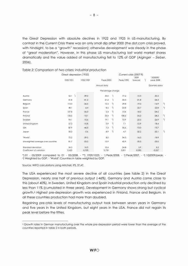
the Great Depression with absolute declines in 1922 and 1925 in US-manufacturing. By
contrast in the Current Crisis there was an only small dip after 2000 (the dot.com crisis proved,
with hindsight, to be a “growth” recession); otherwise development was steady in the phase
of “great moderation”. However, in this phase US manufacturing lost world market shares
dramatically and the value added of manufacturing fell to 12% of GDP (Aiginger Sieber,
2006).
Table 2: Comparison of two crises: industrial production
1929/1921 1932/1929 Peak/2000 Peak/1990
2009
forecast *)
2Q2009/
peak 2008
Quarterly data
Austria 52.1 *) -39.0 33.0 1) 77.2 -15.3 -20.5
Germany 51.8 -41.2 21.2 1) 33.5 -21.8 -24.3
Belgium 113.0 -36.5 12.3 2) 29.8 -19.0 -16.9 3)
Spain 48.1 -6.4 8.5 2) 23.8 -22.7 -22.8 3)
France 127.8 -26.0 2.4 2) 13.4 -18.2 -24.6
Finland 134.6 -13.1 25.4 2) 108.6 -24.3 -28.2 3)
Sweden 94.1 -10.6 19.1 2) 73.9 -22.3 -26.9 3)
United Kingdom 57.3 -10.8 0.9 2) 7.1 -12.9 -18.4
USA 87.9 -46.0 7.3 2) 56.6 -13.0 -15.7
Japan 50.0 -2.6 8.9 2) 4.7 -32.2 -32.1 3)
"World" 72.2 -29.5 8.0 34.3 -16.5 -18.9
Unweighted average over countries 81.7 -23.2 13.9 42.9 -20.2 -23.0
Standard deviation 34.3 16.3 10.4 34.8 5.9 5.2
Coefficient of variation 0.420 -0.703 0.750 0.811 -0.290 -0.227
Great depression (1932) Current crisis (2007 ff)
Percentage change
Annual data
*) 01 - 05/2009 compared to 01 - 05/2008. - **) 1929/1023. - 1) Peak/2008. - 2) Peak/2007. - 3) 1Q2009/peak. - 4) Weighted by GDP. - "World": Countries in table weighted by GDP.
Source: WIFO calculations using Mitchell, IFS, ST.AT.
The USA experienced the most severe decline of all countries (see table 2) in the Great
Depression, nearly one half of previous output (-46%). Germany and Austria came close to
this (about 40%). In Sweden, United Kingdom and Spain industrial production only declined by
less than 11% (cumulated in three years). Development in Germany shows strong but cyclical
growth.6 Highest pre-depression growth was experienced in Finland, France and Belgium. In
all these countries production had more than doubled.
Regaining pre-crisis levels of manufacturing output took between seven years in Germany
and five years in the United Kingdom, but eight years in the USA. France did not regain its
peak level before the fifties.
6 Growth rates in German manufacturing over the whole pre-depression period were lower than the average of the
countries reported in table 2 in both periods.

– 9 –
Figure 2: Industrial production: boom and decline
1408.89715
1408.89715
1408.89715
1408.89715
1408.89715
1408.89715
World and Austria
World and Japan
Great Depression (1929=100) Current crisis (2008=100)World and USA
World and United Kingdom
World and Germany
World and Sweden
50
60
70
80
90
100
110
120
130
1990 1992 1994 1996 1998 2000 2002 2004 2006 2008 2010
2000/2008: + 5.0%
Trough 2009/peak: - 13.0%
World
USA
50
60
70
80
90
100
110
120
130
1920 1922 1924 1926 1928 1930 1932 1934 1936 1938 1940
1921/1929: + 87.9%
1929/1932: - 46.0%
World
USA
50
60
70
80
90
100
110
120
130
1990 1992 1994 1996 1998 2000 2002 2004 2006 2008 2010
2000/2008: - 1.8%
Trough 2009/peak: - 12.9%
World
United Kingdom
50
60
70
80
90
100
110
120
130
1920 1922 1924 1926 1928 1930 1932 1934 1936 1938 1940
1921/1929: + 57.3%
1929/1932: - 10.8%
World
United Kingdom
50
60
70
80
90
100
110
120
130
1990 1992 1994 1996 1998 2000 2002 2004 2006 2008 2010
2000/2008: + 21.2%
Trough 2009/peak: - 21.8%
World
Germany
50
60
70
80
90
100
110
120
130
1920 1922 1924 1926 1928 1930 1932 1934 1936 1938 1940
1921/1929: + 51.8%
1929/1932: - 41.2%
World
Germany
50
60
70
80
90
100
110
120
130
1990 1992 1994 1996 1998 2000 2002 2004 2006 2008 2010
2000/2008: + 15.1%
Trough 2009/peak: - 22.3%
WorldSweden
50
60
70
80
90
100
110
120
130
1920 1922 1924 1926 1928 1930 1932 1934 1936 1938 1940
1921/1929: + 94.1%
1929/1932: - 10.6%
World
Sweden
50
60
70
80
90
100
110
120
130
1990 1992 1994 1996 1998 2000 2002 2004 2006 2008 2010
2000/2008: + 33.0%
Trough 2009/peak: - 15.3%
World
Austria
50
60
70
80
90
100
110
120
130
1920 1922 1924 1926 1928 1930 1932 1934 1936 1938 1940
1923/1929: + 52.1%
1929/1932: - 39.0%
World
Austria
50
60
70
80
90
100
110
120
130
1990 1992 1994 1996 1998 2000 2002 2004 2006 2008 2010
2000/2008: + 5.5%
Trough 2009/peak: - 32.1%
World
Japan
50
60
70
80
90
100
110
120
130
1920 1922 1924 1926 1928 1930 1932 1934 1936 1938 1940
1921/1929: + 50.0%
1929/1932: - 2.6%
World
Japan

– 10 –
The Current Crisis
Finland and Austria had the highest growth in the build-up to the Current Crisis. Spain, France,
and the United Kingdom had only single digit cumulated growth rates over nearly 20 years. In
the Current Crisis we first look at annual data (using the decline between January and May
2009 as a forecast for the annual decline in 2009 and assuming that in 2010 there will be no
further decline in manufacturing production).
On this basis the average decline in manufacturing using annual data amounts to 20%. The
USA see the least decline, maybe as a result of previous deindustrialization, namely 13%. The
highest decline occurred in Sweden and Finland (22% and 24% respectively), as countries
which had a stable or increasing share of industrial output (against the trend for industrialized
countries). On the basis of quarterly data, the average decrease in the reported countries
was 23% (between 2Q2/2009 and the peak in some quarters of 2008).
In the Current Crisis, as opposed to in the Great Depression, the decline was much more
synchronized: the coefficient of variation is 0.2 for quarterly as well as annual data, nearly one
third of that of the Great Depression which was 0.7. This reflects globalized markets.7
Summary
For manufacturing the current decline, if it really does stop in 2009, has been milder than in
the Great Depression, although the difference is less for manufacturing than for total GDP.
The decline occurred over a shorter period of time four to six quarters so that the speed of
decline at the start of the crisis had been as fast, and in some countries faster, than in the
Great Depression, definitely faster in August to October 2008. 8
2.3 Exports larger decline for a few months
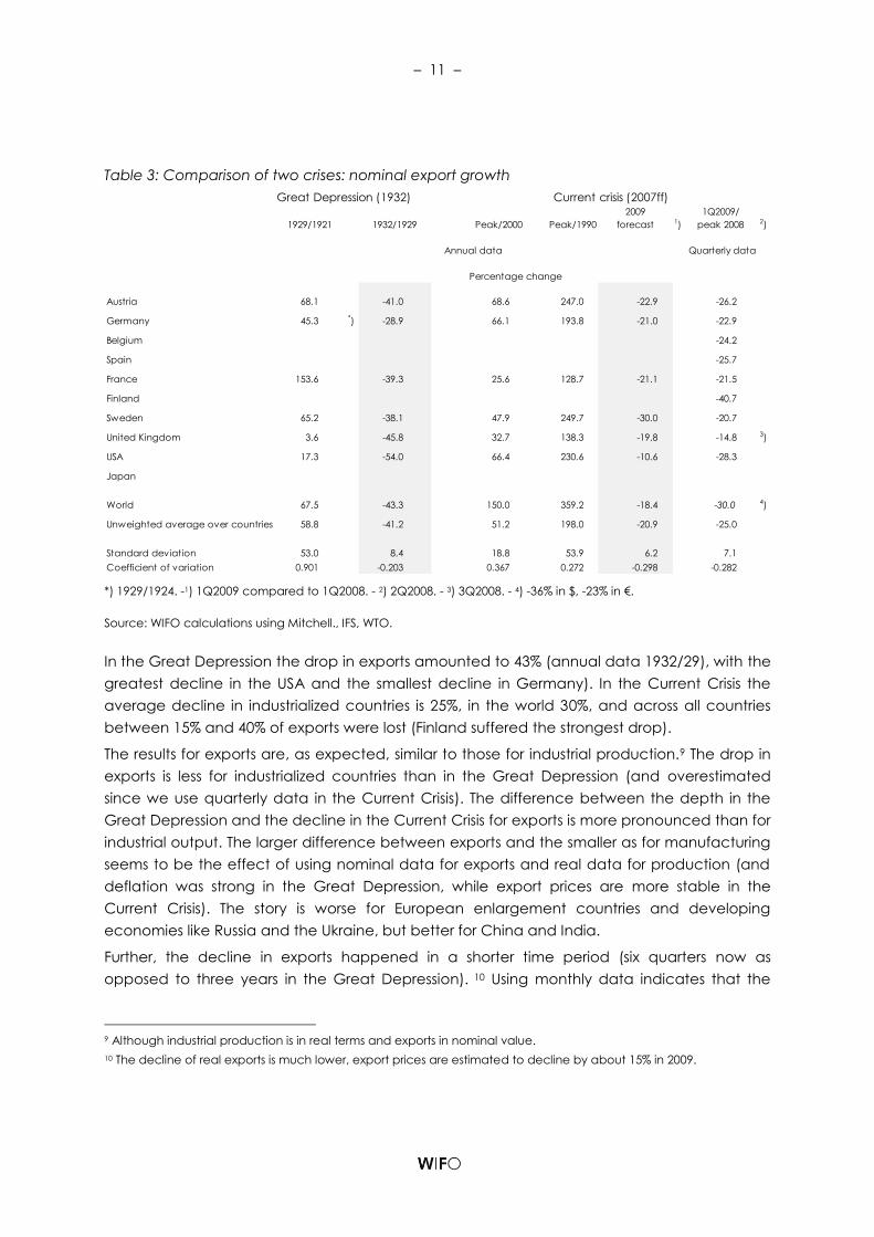
Exports (at nominal rates, national currencies) increased in industrialized countries by more
than 50% in the both build-up periods of the Great Depression, but quadrupled in the build-up
phase of the Current Crisis (table 3, figure 3). Cross country differences were enormous in the
decade preceding the Great Depression (between a near stagnation value of 4% in the
United Kingdom and more than twofold in France). Cross country export growth was more
similar between 1990 and 2008 (with the lowest growth in France and the highest in Sweden
and Austria).
7 Cross country variations in growth were lower in the build-up phase of the Great Depression (average growth 82%,
standard deviation 34, coefficient of variation 0.42), than in the build-up of the Current Crisis (43%, 35, 0.81
respectively).
8 This evidence is reflected also in Eichengreen - O´Rourke (2009) which shows that in the first 12 months of the crisis
(calculated to start in June 1929 and April 2008) on the world scale the decline was surprisingly similar in both
depressions (and stronger between April 2008 and October 2008). Data available in September 2009, shows the
decline to have been less in the US, but stronger in Italy and France. We do not have monthly data for the thirties
currently in the WIFO Long-term Database.
– 11 –
Table 3: Comparison of two crises: nominal export growth
Great Depression (1932)
1929/1921 1932/1929 Peak/2000 Peak/1990
2009
forecast 1)
1Q2009/
peak 2008 2)
Quarterly data
Austria 68.1 -41.0 68.6 247.0 -22.9 -26.2
Germany 45.3 *) -28.9 66.1 193.8 -21.0 -22.9
Belgium -24.2
Spain -25.7
France 153.6 -39.3 25.6 128.7 -21.1 -21.5
Finland -40.7
Sweden 65.2 -38.1 47.9 249.7 -30.0 -20.7
United Kingdom 3.6 -45.8 32.7 138.3 -19.8 -14.8 3)
USA 17.3 -54.0 66.4 230.6 -10.6 -28.3
Japan
World 67.5 -43.3 150.0 359.2 -18.4 -30.0 4)
Unweighted average over countries 58.8 -41.2 51.2 198.0 -20.9 -25.0
Standard deviation 53.0 8.4 18.8 53.9 6.2 7.1
Coefficient of variation 0.901 -0.203 0.367 0.272 -0.298 -0.282
Current crisis (2007ff)
Percentage change
Annual data
*) 1929/1924. -1) 1Q2009 compared to 1Q2008. - 2) 2Q2008. - 3) 3Q2008. - 4) -36% in $, -23% in €.
Source: WIFO calculations using Mitchell., IFS, WTO.
In the Great Depression the drop in exports amounted to 43% (annual data 1932/29), with the
greatest decline in the USA and the smallest decline in Germany). In the Current Crisis the
average decline in industrialized countries is 25%, in the world 30%, and across all countries
between 15% and 40% of exports were lost (Finland suffered the strongest drop).
The results for exports are, as expected, similar to those for industrial production.9 The drop in
exports is less for industrialized countries than in the Great Depression (and overestimated
since we use quarterly data in the Current Crisis). The difference between the depth in the
Great Depression and the decline in the Current Crisis for exports is more pronounced than for
industrial output. The larger difference between exports and the smaller as for manufacturing
seems to be the effect of using nominal data for exports and real data for production (and
deflation was strong in the Great Depression, while export prices are more stable in the
Current Crisis). The story is worse for European enlargement countries and developing
economies like Russia and the Ukraine, but better for China and India.
Further, the decline in exports happened in a shorter time period (six quarters now as
opposed to three years in the Great Depression). 10 Using monthly data indicates that the
9 Although industrial production is in real terms and exports in nominal value.
10 The decline of real exports is much lower, export prices are estimated to decline by about 15% in 2009.

– 12 –
drop of exports between September 2008 and February 2009 was stronger in this recession.
The lines crossed in July 2009.11
Figure 3: Export growth: boom and decline
1408.89715
1408.89715
1408.89715
1408.89715
1408.89715
World and Austria
Great Depression (1929=100) Current crisis (2008=100)World and USA
World and United Kingdom
World and Germany
World and Sweden
20
40
60
80
100
120
140
1990 1992 1994 1996 1998 2000 2002 2004 2006 2008 2010
2000/2008: + 66.4%
Trough 2009/peak: - 22.9%
World
USA
20
40
60
80
100
120
140
1920 1922 1924 1926 1928 1930 1932 1934 1936 1938 1940
1921/1929: + 17.3%
1929/1932: - 69.5%
World
USA
20
40
60
80
100
120
140
1990 1992 1994 1996 1998 2000 2002 2004 2006 2008 2010
2000/2008: + 32.7%
Trough 2009/peak: - 19.8%
World
United Kingdom
20
40
60
80
100
120
140
1920 1922 1924 1926 1928 1930 1932 1934 1936 1938 1940
1921/1929: + 3.6%
1929/1932: - 50.4%
World
United Kingdom
20
40
60
80
100
120
140
1990 1992 1994 1996 1998 2000 2002 2004 2006 2008 2010
2000/2008: + 66.1%
Trough 2009/peak: - 21.0%
World
Germany
20
40
60
80
100
120
140
1920 1922 1924 1926 1928 1930 1932 1934 1936 1938 1940
1923/1929: + 121.0%
1929/1932: - 57.4%
World
Germany
20
40
60
80
100
120
140
1990 1992 1994 1996 1998 2000 2002 2004 2006 2008 2010
2000/2008: + 47.9%
Trough 2009/peak: - 30.0%
World
Sweden
20
40
60
80
100
120
140
1920 1922 1924 1926 1928 1930 1932 1934 1936 1938 1940
1921/1929: + 65.2%
1929/1932: - 47.7%
World
Sweden
20
40
60
80
100
120
140
1990 1992 1994 1996 1998 2000 2002 2004 2006 2008 2010
2000/2008: + 68.6%
Trough 2009/peak: - 22.9%
World
Austria
20
40
60
80
100
120
140
1920 1922 1924 1926 1928 1930 1932 1934 1936 1938 1940
1921/1929: + 68.1%
1929/1932: - 65.1%
World
Austria
11 Interestingly in the Great Depression world trade had continued to increase up to December 1929 (indicating that
the Great Depression has not been trigger by a breakdown of world trade (see Eichengreen O’Rourke, 2009). They
start their figure with April 1929 which may be problematic since trade increased up to December.

– 13 –
2.4 The Stock Market
To analyze the development of the stock market we use quarterly data (end of the quarter
prices)12. The S&P index is our starting point to describe development in the USA since it is the
best documented index, for Germany we use the DAX and its predecessor, for the United
Kingdom the FTSE and its predecessor, for Japan the Nikkei and its predecessor. We construct
a synthetic “world” index by weighing the indices according to the GDP share of each
country in world GDP (without Japan).
Table 4: Comparison of two crises: stock markets
Peak 1929/
trough 1921
Trough 1932/
peak 1929
Peak 1932/
trough 1930 1)
Peak 2007/
peak 2000
Peak 2007/
trough 2003
Trough 2008/
peak 2007
Austria -45.6 4.7 330.9 318.6 -65.2
Germany -83.9 -62.1 3.5 14.1 237.7 -51.7
Belgium
Spain
France 335.3 -56.2 3.2 -6.1 131.2 -53.6
Finland
Sweden
United Kingdom -49.3 -4.1 72.6 191.1 -44.7
USA 377.9 -84.8 11.9 3.1 78.8 -50.0
Japan -34.2 15.2 127.5 -55.3
"World" -68.9 5.0 29.3 130.1 -47.7
Unweighted average over countries 209.8 -59.6 82.9 191.5 -53.0
Standard deviation 255.2 15.4 142.0 93.0 7.5
Coefficient of variation 1.217 -0.259 1.712 0.486 -0.142
Current crisis (2007ff)
Quarterly data; percentage change
Great Depression (1932)
1) Rebounds after the trough (no rebound in the United Kingdom). - "World": USA, United Kingdom, Germany and
France weighted by GDP.
Source: WIFO calculations using http://www.econ.yale.edu/~shiller/data.htm for the USA;
http://stooq.de/q/d/?s=nikkei&c=0&i=m for Japan; NBER Macrohistory Database;
http://finance.yahoo.com/q/hp?s=^CDAXX, Gregor Gielen (1960-1979) for Germany; NBER Macrohistory Database;
http://stooq.de/q/d/?s=cac40, IMF for France; - League of Nations; http://stooq.de/q/d/?s=ftse250&c=0&i=m, IMF for
the United Kingdom; Monatsberichte des Österreichischen Institues für Konjunkturforschung;
http://stooq.de/q/d/?s=atx&c=0&i=m , IMF for Austria.
12 Even monthly data was available, but we stick to quarterly data, which we think to be the best middle path
between annual data which can hide important developments and monthly data which exhibit a lot of noise.

– 14 –
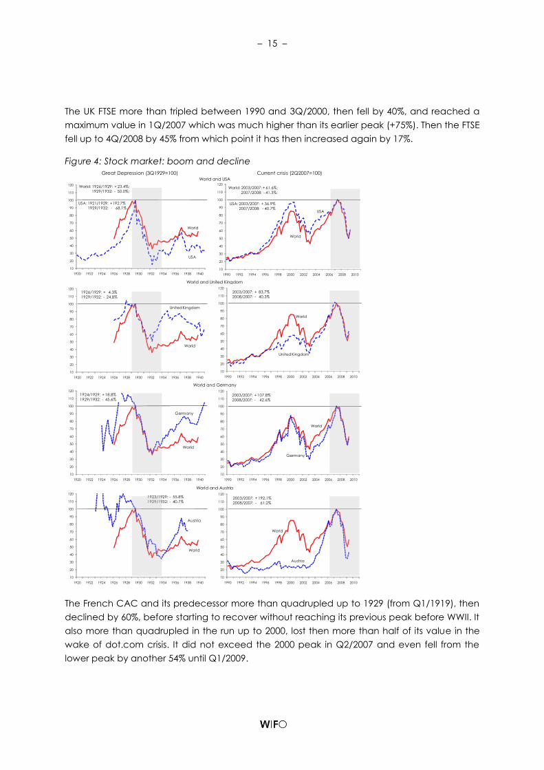
Build-up period and decline
The build-up periods have some features in common and some are different.
In the USA the stock market quadrupled between 1921(2Q) and its peak in 1929 (3Q). There
had been no bust period in these ten years, only a few quarters with stagnation or relatively
small declines (at least small for markets that are volatile). The increase accelerated, and
came near to 50% in the four quarters preceding the peak.
In the Current Crisis the last ten years were more turbulent. Stock market prices had reached
their peak in 2Q/2001, and then declined by 30% by 1Q/2003. The US stock market then
recovered and exceeded its previous peak of 2000 by 6% in 2Q/2007. In the period before
2000 there had been a strong and long increase and indeed a quadrupling in value since
1990.
In the Great Depression the S&P index dropped from 100 (3Q/1929) to 15 (2Q/1932). This
happened over a period of only eleven quarters. Then came a temporary peak in 1936/37,
but the previous peak was reached only in 3Q/1954. In the Current Crisis the maximum
decline is 50% from the peak in 2Q/2007. The minimum level was reached in 1Q/2009, seven
quarters after the peak. Since then the Standard & Poor index recovered by 20% (on the
quarterly basis; somewhat more strongly for monthly data: 30%).
Country differences
In Japan the fall of stock prices was relatively mild in the Great Depression (-34%). The
development of the Japanese stock market, as reflected by the Nikkei, is very different over
the last 20 years to the other countries. It quadrupled between 3Q/1982 and 4Q/1989, and
returned with a lot of short-term volatility to its 1983 value at the beginning of 2002 and 2003. It
then doubled reaching a peak in 2Q/2007, dropped to the 1983 level again and recovered
slightly during 2009. In short it is very volatile and does not show a growth trend. Japan is the
only country, other than Austria, where stock prices did decrease more strongly in the Current
Crisis.13
Germany did experience a bumpy increase before the Great Depression, with a strong
decline between 1Q/1924 and 4Q/1925. Then the index doubled reaching its peak in
2Q/1928. Between this peak and 2Q/1932 it declined to less than 30% of its maximum. It did
not recover before 4Q/1940 where the series is interrupted.
The DAX tripled between 1990 and 1Q/2000, fell to less than half of this peak value in
1Q/2003, reached a new maximum 14% above the old peak in 2Q/2007. It fell to 48% of the
2Q/2007 value in 1Q/2009 and since then recovered by 19% on a quarterly basis and by 45%
on a monthly basis (up to end of August 2009).
13 If we weight together all the six indices in table 4 (weighted by GDP) the stock prices decline by 69% between 1929
and 1932 and by 44% in the Current Crisis. Stock prices rebounded by 45% up to August 2009 (unweighted average).
– 15 –
The UK FTSE more than tripled between 1990 and 3Q/2000, then fell by 40%, and reached a
maximum value in 1Q/2007 which was much higher than its earlier peak (+75%). Then the FTSE
fell up to 4Q/2008 by 45% from which point it has then increased again by 17%.
Figure 4: Stock market: boom and decline
1408.89715
1408.89715
1408.89715
World and Austria
Great Depression (3Q1929=100) Current crisis (2Q2007=100)World and USA
World and United Kingdom
World and Germany
10
20
30
40
50
60
70
80
90
100
110
120
1990 1992 1994 1996 1998 2000 2002 2004 2006 2008 2010
World
USA
World: 2003/2007: + 61.6%;
2007/2008: - 41.3%;
USA: 2003/2007: + 36.9%
2007/2008: - 40.7%
10
20
30
40
50
60
70
80
90
100
110
120
1920 1922 1924 1926 1928 1930 1932 1934 1936 1938 1940
USA
World: 1926/1929: + 23.4%;
1929/1932: - 50.0%;
USA: 1921/1929: +192.7%
1929/1932: - 68.1%
World
10
20
30
40
50
60
70
80
90
100
110
120
1990 1992 1994 1996 1998 2000 2002 2004 2006 2008 2010
United Kingdom
World
2003/2007: + 83.7%
2008/2007: - 40.3%
10
20
30
40
50
60
70
80
90
100
110
120
1920 1922 1924 1926 1928 1930 1932 1934 1936 1938 1940
World
United Kingdom
1926/1929: + 4.3%
1929/1932: - 24.8%
10
20
30
40
50
60
70
80
90
100
110
120
1990 1992 1994 1996 1998 2000 2002 2004 2006 2008 2010
Germany
World
2003/2007: + 107.8%
2008/2007: - 42.6%
10
20
30
40
50
60
70
80
90
100
110
120
1920 1922 1924 1926 1928 1930 1932 1934 1936 1938 1940
World
Germany
1924/1929: + 18.8%
1929/1932: - 45.6%
10
20
30
40
50
60
70
80
90
100
110
120
1990 1992 1994 1996 1998 2000 2002 2004 2006 2008 2010
Austria
World
2003/2007: + 192.1%
2008/2007: - 61.2%
10
20
30
40
50
60
70
80
90
100
110
120
1920 1922 1924 1926 1928 1930 1932 1934 1936 1938 1940
World
Austria
1923/1929: - 55.8%
1929/1932: - 40.7%
The French CAC and its predecessor more than quadrupled up to 1929 (from Q1/1919), then
declined by 60%, before starting to recover without reaching its previous peak before WWII. It
also more than quadrupled in the run up to 2000, lost then more than half of its value in the
wake of dot.com crisis. It did not exceed the 2000 peak in Q2/2007 and even fell from the
lower peak by another 54% until Q1/2009.

– 16 –
Table 5: Comparison of two crises: employment
1929 1929/1921 1929/1912 1932/1929 2008 2008/2000 2008/1990
2009
forecast
Trough 2009/
peak 2008
Quarterly data
1000 persons 1000 persons
Austria 2032 -6.0 -10.9 -17.2 3420.5 9.2 16.8 -2.7 -1.0 2)
Germany -28.9 38879.7 7.3 7.4 -1.5 -0.8 3)
Belgium
Spain
France -19.1 1) 25914.1 7.2 14.5 -2.2 -0.4 4)
Finland
Sweden 4602.8 10.7 2.7 -2.4 -2.7 5)
United Kingdom 19479 8.8 -2.1 -2.3 29447.7 7.1 9.6 -2.4 -1.1 6)
USA 47600 28.3 31.5 -13.7 145362.5 6.2 22.4 -3.5 -3.9 7)
Japan -3.0 -2.4 8)
Sum of countries 69111.0 10.4 6.2 -16.3 247627.2 7.9 12.2 -2.5 -1.6
Standard deviation 22991.4 17.2 22.4 9.6 52902.9 1.7 7.1 0.7 1.4
Coefficient of variation 0.998 1.658 3.616 -0.590 1.282 0.211 0.580 -0.267 -0.824
Annual data
Percentage change
Annual data
Percentage change
Current crisis (2007ff)Great Depression (1932)
1) 1932/1930. - 2) 1Q2009/4Q2008. - 3) 1Q2009/1Q2008. - 4) 2Q2009/4Q2008. - 5) 2Q2009/3q2008. - 6) 1Q2009/2Q2008. - 7) 2Q2009/4Q2007. - 8) 2Q2009/2Q2007.
Source: WIFO calculations using The Economist; Economic Statistics 1900 -1983, 1985 and OECD; Eurostat.
In Austria the decline of the stock market in the Current Crisis has actually been steeper than
between 1929 and 1932, namely 64% and 46% respectively (see table 4). This is due to several
facts which are specific to Austria: the decline in the stock market was rather mild in the
Great Depression (which is surprising since Austria was a country severely hit in the Great
Depression). Secondly, Austria had an extreme boom between 2000 and 2007 (the ATX
quadrupled in comparison with a twofold increase in the unweighted average of other
countries). Thirdly, the debate about the engagement of Austrian firms in the East led do
heavy disinvestment during the Current Crisis. However, Austria does have the highest
rebound level since February 2009. These variations to the general trends demonstrate a
rather thin market and a lack of specific information for worldwide investors about the
Austrian markets (substituted by rather general assessments of country risks).
If we weight together the US S&P, the German Dax, the French CAC and the UK FTSE 250, we
get a steep decline for this composite “World Index”. In the Great Depression it declined by
69% and in the Current Crisis only by 44% (on the basis of quarterly data). On an individual
country basis the decline in the Current Crisis is actually very similar in the four countries (in
each country it falls between 42% and 47%).
The peak in 2007 had been 29% higher than the 2000 peak, however with large differences
between countries (lower in France, higher in the United Kingdom). If the peak in 2007 is
compared to the “interim trough” in 2003 (after the dot.com crisis) stock prices more than
doubled in the composite index. The rebound since the lowest level (February 2009, now
– 17 –
measured on a monthly scale) has been 33% on average again very similar across the four
countries.14
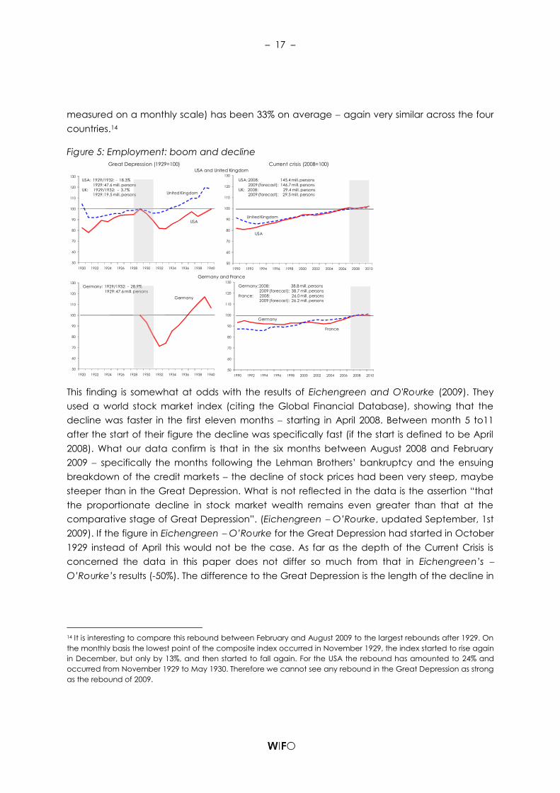
Figure 5: Employment: boom and decline
1408.89715
1408.89715
Great Depression (1929=100) Current crisis (2008=100)USA and United Kingdom
Germany and France
50
60
70
80
90
100
110
120
130
1990 1992 1994 1996 1998 2000 2002 2004 2006 2008 2010
USA: 2008: 145.4 mill. persons
2009 (forecast): 146.7 mill. persons
UK: 2008: 29.4 mill. persons2009 (forecast): 29.5 mill. persons
USA
United Kingdom
50
60
70
80
90
100
110
120
130
1920 1922 1924 1926 1928 1930 1932 1934 1936 1938 1940
USA: 1929/1932: - 18.3%
1929: 47.6 mill. persons
UK: 1929/1932: - 3.7%1929: 19.5 mill. persons United Kingdom
USA
50
60
70
80
90
100
110
120
130
1990 1992 1994 1996 1998 2000 2002 2004 2006 2008 2010
France
Germany
Germany: 2008: 38.8 mill. persons
2009 (forecast): 38.7 mill. persons
France: 2008: 26.0 mill. persons2009 (forecast): 26.2 mill. persons
50
60
70
80
90
100
110
120
130
1920 1922 1924 1926 1928 1930 1932 1934 1936 1938 1940
Germany
Germany: 1929/1932: - 28.9%
1929: 47.6 mill. persons
This finding is somewhat at odds with the results of Eichengreen and O'Rourke (2009). They
used a world stock market index (citing the Global Financial Database), showing that the
decline was faster in the first eleven months starting in April 2008. Between month 5 to11
after the start of their figure the decline was specifically fast (if the start is defined to be April
2008). What our data confirm is that in the six months between August 2008 and February
2009 specifically the months following the Lehman Brothers’ bankruptcy and the ensuing
breakdown of the credit markets the decline of stock prices had been very steep, maybe
steeper than in the Great Depression. What is not reflected in the data is the assertion “that
the proportionate decline in stock market wealth remains even greater than that at the
comparative stage of Great Depression”. (Eichengreen O’Rourke, updated September, 1st
2009). If the figure in Eichengreen O’Rourke for the Great Depression had started in October
1929 instead of April this would not be the case. As far as the depth of the Current Crisis is
concerned the data in this paper does not differ so much from that in Eichengreen’s
O’Rourke’s results (-50%). The difference to the Great Depression is the length of the decline in
14 It is interesting to compare this rebound between February and August 2009 to the largest rebounds after 1929. On
the monthly basis the lowest point of the composite index occurred in November 1929, the index started to rise again
in December, but only by 13%, and then started to fall again. For the USA the rebound has amounted to 24% and
occurred from November 1929 to May 1930. Therefore we cannot see any rebound in the Great Depression as strong
as the rebound of 2009.
– 18 –
the Current Crisis This ultimately depends on whether we have already reached the trough or
whether a second wave might still come.15
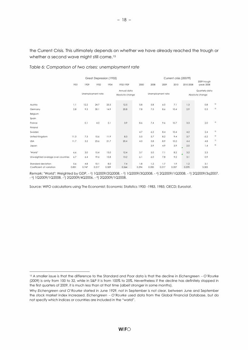
Table 6: Comparison of two crises: unemployment rate
1921 1929 1932 1934 1932-1929 2000 2008 2009 2010 2010-2008
2009 trough
-peak 2008
Quarterly data
Absolute change
Austria 1.1 12.2 24.7 25.5 12.5 5.8 5.8 6.0 7.1 1.3 0.8 2)
Germany 2.8 9.3 30.1 14.9 20.8 7.8 7.5 8.6 10.4 2.9 0.3 3)
Belgium
Spain
France 0.1 4.0 5.1 3.9 8.6 7.4 9.6 10.7 3.3 2.0 4)
Finland
Sweden 4.7 6.2 8.4 10.4 4.2 2.4 5)
United Kingdom 11.3 7.3 15.6 11.9 8.3 5.5 5.7 8.2 9.4 3.7 -5.2 6)
USA 11.7 3.2 23.6 21.7 20.4 4.0 5.8 8.9 10.2 4.4 4.8 7)
Japan 3.9 4.9 5.9 2.0 1.4 8)
"World" 6.6 3.0 15.4 13.0 12.4 3.7 5.0 7.1 8.2 3.2 2.3
Unweighted average over countries 6.7 6.4 19.6 15.8 13.2 6.1 6.0 7.8 9.2 3.1 0.9
Standard deviation 5.6 4.8 10.1 8.0 7.4 1.8 1.2 1.7 1.9 1.2 3.1
Coefficient of variation 0.831 0.747 0.517 0.509 0.564 0.294 0.200 0.217 0.207 0.370 3.305
Current crisis (2007ff)
Annual data
Unemployment rate Unemployment rate Absolute change
Great Depression (1932)
Remark: "World": Weighted by GDP. - 2) 1Q2009/2Q2008. - 3) 1Q2009/3Q2008. - 4) 2Q2009/1Q2008. - 5) 2Q2009/3q2007.
- 6) 1Q2009/1Q2008. -7) 2Q2009/4Q2006. - 8) 2Q2009/1Q2008.
Source: WIFO calculations using The Economist; Economic Statistics 1900 -1983, 1985; OECD; Eurostat.
15 A smaller issue is that the difference to the Standard and Poor data is that the decline in Eichengreen O’Rourke
(2009) is only from 100 to 32, while in S&P it is from 100% to 25%. Nevertheless if the decline has definitely stopped in
the first quarters of 2009, it is much less than at that time (albeit stronger in some months).
Why Eichengreen and O’Rourke started in June 1929, not in September is not clear, between June and September
the stock market index increased. Eichengreen O’Rourke used data from the Global Financial Database, but do
not specify which indices or countries are included in the “world”.

– 19 –
Figure 6: Unemployment rate: boom and decline
1408.89715
1408.89715
Great Depression Current crisisUSA and United Kingdom
Germany and France
0
5
10
15
20
25
30
1990 1992 1994 1996 1998 2000 2002 2004 2006 2008 2010
USA: 2008: 5.8%
2009 (forecast): 8.9%
UK: 2008: 5.7%2009 (forecast): 8.2%
USA
United Kingdom
0
5
10
15
20
25
30
1920 1922 1924 1926 1928 1930 1932 1934 1936 1938 1940
USA: 1929: 3.2%
1932: 23.6%
UK: 1929: 7.3%1932: 15.6%
United Kingdom
USA
0
5
10
15
20
25
30
1990 1992 1994 1996 1998 2000 2002 2004 2006 2008 2010
France
Germany
Germany: 2008: 7.5%
2009 (forecast): 8.6%
France: 2008: 7.4%2009 (forecast): 9.6%
0
5
10
15
20
25
30
1920 1922 1924 1926 1928 1930 1932 1934 1936 1938 1940
Germany
Germany: 1929: 9.3%
1932: 30.1%
France: 1930: 0.1%1932: 4.0%
France
3. Policy response
3.1 Monetary policy: mildly, restrictive vs. aggressively, expansionary
Monetary policy and its constraints in the Great Depression
This is not the place to give evidence on the causality between monetary policy and the
depression, neither whether restrictive monetary policy “caused” the Great Depression, nor
whether monetary policy was too loose following the dot.com crisis in 2003. Here we just
present stylized facts about monetary variables, mainly following Bernanke (2004) and
Eichengreen Sachs (1985) for the Great Depression (thus concentrating to some degree
unduly on the US policy) and the OECD (2009) for the Current Crisis. Additionally we present
stylized facts for inflation, interest rates and money supply for the two crises.
Friedman and Schwartz (1963) argue that the causal link for the Great Depression ran from
monetary policy to declining prices and output, thus giving poor policy making the blame for
the start of the Great Depression, which was then aggravated due to the breakdown of the
banking system. Other authors stress the strong decline in US consumption in 1930 (Temin,
1976). Galbraith (1954) names “bad distribution of income, …. bad corporate structure, ….
bad banking structure…. dubious state of foreign balance … and poor state of economic
intelligence”. A large part of newer research stresses the role that the gold standard had
played (Eichengreen O’Rourke, 2009, Bernanke, 2004). The gold standard was re-enacted
after WWI in most countries.16 Under the gold standard each country had to defend its
currency value and the money supply could not increase independently from the gold
16 With exception of Spain which could not do it due to internal turmoil.

– 20 –
reserves (for given multipliers). The important role of this, with hindsight, flawed international
monetary system prevented an active anti cyclical monetary policy. The importance of the
gold standard for the length of the crisis is highlighted by the fact that “countries abandoning
the gold standard were able to reflate their money supply and price levels and did so with
some delay, while countries remaining on the gold were forced into further deflation”
(Bernanke, 2004, p. 8). Countries with gold inflow tried to sterilize it, in countries with gold
outflow the monetary base declined nearly automatically. Thus it was not the gold standard
per se but the restrictive asymmetric handling of the regime, which made the Great
Depression longer.
Table 7: Comparison of two crises: inflation/deflation (consumer prices)
1927 1928 1929 1930 1931 1932 1933 1932/1929 2006 2007 2008 2009 2Q2009/3Q2008
Percentage
price
change Forecast Quarterly change
Austria 2.2 2.1 3.1 0.0 -5.0 2.1 -2.1 -3.0 1.5 2.2 3.2 1.1 0.0
Germany 4.3 3.1 1.0 -4.0 -8.3 -11.4 -1.3 -22.0 1.9 2.8 2.6 0.7 -0.6
Belgium 1.2 -0.7
Spain 1.4 -0.7
France 4.4 0.0 6.4 1.0 -4.0 -9.3 -3.4 -12.0 2.5 2.5 2.8 0.9 -0.3
Finland 1.1 1.2
Sweden -1.2 0.6 -1.2 -3.6 -3.1 -1.3 -2.6 -7.7 1.3 2.0 3.4 0.7 1.4
United Kingdom -2.9 -1.0 -1.0 -4.0 -6.3 -2.2 -3.4 -12.0 -1.3 1.4 4.0 1.3 0.8
USA -1.7 -1.1 0.0 -2.9 -8.3 -10.4 -5.1 -20.2 0.2 1.5 3.9 0.3 -2.3
Japan -0.5 -1.9
"World" -0.1 -0.2 0.6 -2.2 -5.8 -6.9 -3.1 -14.1 0.4 1.5 2.8 0.5 -1.1
Unweighted average over countries 0.9 0.6 1.4 -2.2 -5.8 -5.4 -3.0 -12.8 1.0 2.1 3.3 1.0 -0.1
Standard deviation 3.2 1.7 2.9 2.2 2.2 5.6 1.3 7.2 1.4 0.5 0.5 0.4 1.2
Coefficient of variation 3.667 2.766 2.094 -0.975 -0.379 -1.043 -0.443 -0.565 1.365 0.260 0.163 0.362 -9.952
Change over previous yearChange over previous year
Great Depression (1932) Current crisis (2007ff)
Remark: "World": Weighted by GDP.
Source: WIFO calculations using Mitchell, Eurostat.
As for the start of the Great Depression, the Fed turned contractionary in 1928 to curb stock
market speculation. The US monetary base (money and notes in circulation plus reserves of
banks) fell by 6% between June 1928 and June 1930 despite an inflow of gold into the USA.
Gold also rushed into France (after the Poincaré stabilization). This reduced the amount of
gold available in other countries and forced them into a tight monetary policy.
The second stage of the crisis occurred in 1931 due to the breakdown of banks
(“Creditanstalt” in Austria etc.) which lead to waves of bank crises and an exchange rate
crisis. The monetary base declined even further.
Interest rates remained constant in nominal terms, but on levels of 5.3% and 5.4% in the first
three years of the crisis, then falling slightly to about 4% in the next four years. Due to the
falling price levels for goods (deflation), ex post real rates amounted to 17% in 1929/1930
(Bernanke, 2004). These extraordinary high rates affected investment and consumption. Real

– 21 –
rates then dropped to 9.4%, 6.5% and 2.8%. At such interest rates, together with declining
demand, excess capacities and a high degree of uncertainty, it is clear that investment and
consumption would decline. Debt inflation, falling assets and commodity prices increased the
burden on all debtors, forcing them to sell assets etc.
Figure 7: Inflation: boom and decline
1408.89715
1408.89715
Great Depression (1929=100) Current crisis (2008=100)USA and United Kingdom
Germany and France
50
60
70
80
90
100
110
120
130
1990 1992 1994 1996 1998 2000 2002 2004 2006 2008 2010
USA: 2000/2008: + 25.0%
2009 (forecast): - 0.7%
UK: 2000/2008: + 26.2%2009 (forecast): + 1.0%
USA
United Kingdom
50
60
70
80
90
100
110
120
130
1920 1922 1924 1926 1928 1930 1932 1934 1936 1938 1940
USA: 1929/1932: - 20.2%
UK: 1929/1932: - 12.0%
United Kingdom
USA
50
60
70
80
90
100
110
120
130
1990 1992 1994 1996 1998 2000 2002 2004 2006 2008 2010
France
Germany
Germany: 2000/2008: + 15.0%
2009 (forecast): + 1.6%
France: 2000/2008: +16.6%2009 (forecast): + 0.2%
50
60
70
80
90
100
110
120
130
1920 1922 1924 1926 1928 1930 1932 1934 1936 1938 1940
Germany
Germany: 1929/1932: - 22.0%
France: 1929/1932: - 12.0%
France
Difference across countries according to Bernanke
Bernanke describes the development of monetary supply using M1, the multiplier (M1/Money
base), the relationship between money base and total reserves (the coverage ratio
determined inter alia by statutory requirements) and the ratio of currency reserves to gold
reserves.
In the USA the M1 decreased by 25% between 1929 and 1933.17 It later only reached its pre-
depression level in 1935. The multiplier decreased even a little more, and did not recover
before 1936. Money base relative to reserves was more or less stable with a significant drop in
1934 from 118 to 66. The ratio of reserves to gold was stable.
In the United Kingdom money supply first rose slightly (+ 2.5%), and dropped in 1931 by 10%.
Then it recovered, but increased strongly as late as 1935 and 1936. The multiplier did not fall
(in fact increased slightly). Base to reserve was stable in 1930, and then it increased, finally
dropping from 117 to 75% (1933) and then further up to 56% (1936).
In France the situation is different. Money supply increased by more than 10% in 1930 and
1931, but then never reached this level again until 1936. The multiplier dropped by a
cumulative 10% in 1929/31 and then remained constant. Base to reserve was more or less
17 This time nominal rates might look more restrictive than they are, since prices were falling, too.

– 22 –
stable (the coverage rate increases strongly in 1935/36). Reserves to gold declined strongly in
each year until 1932 and then remained more or less constant.
Using international comparable data (see table 8) we now outline the relationship between
the money supply (M1) relative to nominal GDP, as well as and inflation as measured by CPI.
USA
Money supply in relation to GDP decreased in the US from a level of between 27% and 28% of
GDP between 1924 and 1928 (specifically 27.2% in 1928), to 25.6% in 1929. In the next three
years money supply increased relatively sharply (also in absolute terms or because of falling
nominal GDP) but dropped again in 1934 and 1935, having a single extreme peak in 1936
and then again a decline. The final take off occurred between 1944 and 1946.
Consumer prices fell by 30% between 1929 and 1933, with the largest decrease in 1932 (10%).
The decline was very small in 1930 (zero in 1929). There had been no inflationary period
before the crisis (in fact +0.5% in 1923 until 1928). There was a deflationary period in 1921/22.
Summing up the results from Bernanke as well as those in table 10 monetary policy could
have been much more expansionary without any fear of inflation, but it was not applied
maybe because of a faint memory of inflation after WWI (1916 to 1920) but probably also
due to the gold standard and the fear of a currency devaluation.18
Germany
In Germany money supply was reduced relative to GDP in 1927, but then increased steadily
and strongly until 1932. Thereafter it decreased until 1936, but increased rather strongly
thereafter.
Inflation had been a little bit higher in the build-up period (and memory of hyperinflation after
WWI still existed). Deflation occurred, reaching its peak in 1932. Moderate price increases
characterized the period of 1934 to 1939.
United Kingdom
In the United Kingdom money supply fell relatively dramatically between 1928 and 1931 (from
34.2% to 29.9% of GDP), then was increased quickly and strongly up to 38.3% of GDP in 1936.
Consumer prices decreased steadily from 1926 (!) to 1934, but never at a two digit rate. The
United Kingdom suspended the gold standard in September 1931.
France
France had a strongly expansionary monetary policy between 1926 and 1935 increasing
money supply from 33.7% of GDP to 73.4%. There was a tiny dip in 1929 (0.9% of GDP) and a
large increase in 1932. Inflation had been rather strong in France before 1929 (6.4% in 1929).
18 The belief that economies will reach their equilibrium fast (without intervention) may have been important, too.

– 23 –
After the Great Depression it looked as if even the very expansionary monetary policy in
France could not have prevented the following five years of falling consumer prices. France
had the largest cumulative price decrease of the reported countries. It devaluated in
October 1936.
Figure 8: Discount rates in major industrialized economies
Note: The dark line represents the main policy rate of the central banks. The light line plots the effective overnight
rate.
Source: IMF, Bloomberg, Bank of Japan, Datastream, ECB. http://dx.doi.org/10.1787/656585873210
The figures presented in Bordo et al. (2001) indicated a considerable increase in the money
supply for the aggregate of the GDP-weighted countries between 1925 and 1929 (+16%
cumulative). In 1929 and 1930 money supply was constant and then dropped for three years
(in 1933 it was back to the 1925 level).

– 24 –
Monetary policy in the current crisis
Monetary policy in the current crisis was very courageous
discount rates were slashed to or near to zero (in Sweden even into the negative range),
after exhausting the scope to reduce interest rates non-conventional measures to
stimulate demand were used;
the breakdown of the inter bank credit market was addressed, and the financial system
was provided with credit and liquidity;
banks and financial institutions were recapitalized using public funds, deposit guarantees
were extended and debt guaranteed;
the problem of toxic assets and of solvency were addressed by ring fencing19 bad banks
(mainly in the United Kingdom) or via temporary public ownership (UK, US, Iceland etc.).
Table 8: Comparison of two crises: money supply (M1)
1929/1921 1932/1929 2007/2000 2007/2003 2008/2007
Austria 4719.0 -16.5 78.4 44.5 8.3
Germany 361.0 -29.4 65.9 29.3 6.7
Belgium
Spain
France 115.9 20.2 84.7 35.1 1.5
Finland
Sweden -3.1 2.9 12.7 2.1 -1.0
United Kingdom -10.0 -2.1 105.4 52.1 -1.4
USA 23.8 -20.8 24.7 4.1 17.2
Japan
"World" 123.5 -11.0 41.5 16.1 8.1
Unweighted average over countries 867.8 -7.6 61.9 27.9 5.2
Standard deviation 1891.9 18.1 36.1 20.7 7.1
Coefficient of variation 2.180 -2.381 0.582 0.744 1.361
Great Depression (1932) Current crisis (2007ff)
Percentage change
Remark: "World": Weighted by GDP.
Source: WIFO calculations using IFS, Bank of England, Risksbank (NOMINAL MONEY SUPPLY (M1) 1807-1935, MILLIONS
OF FRANCS, - SAINT MARC (1983, pp. 36-37).
19 Ring fencing means providing a public guarantee to specific assets after banks have absorbed a lump sum
amount of toxic assets.

– 25 –
Table 11 presents an overview of the financial relief measures, figure 10 an overview of
discount rates and figure 13 shows how unconventional measures have led to the expansion
of the balance sheets of central banks.
As far as conventional measures are concerned the Fed cut its interest rate from a level of 4%
in 2008 (table 9) to a target range of 0% to 0.25% from December 2008. The ECB, starting from
a somewhat lower level, still increased discount rates in June 2008 (to fight inflation) and
subsequently reduced step by step to 1%. The United Kingdom acted last, but then reduced
rates very quickly to ½% in 2008.
Figure 9: Expansion of central banks‘ balance sheets 2000/2009
Source: IMF, Datastream. http://dx.doi.org/10.1787/656585873210
Unconventional measures fall into three categories (OECD, 2009), namely:
providing the banking sector with greater and cheap liquidity.
expanding the money supply through the creation of excess supply (quantitative easing)
intervening directly in broader segments of the credit market
The Fed itself bought commercial papers and securitized products and started to conduct or
expand outright open-market purchases of mortgage backed securities and bonds and
long-term government bonds with the aim of lowering interest rates.
As for the ECB unconventional measures have been more concentrated on easing the
liquidity conditions and increasing the scale of its operations to provide liquidity to financial
institutions. The ECB eased its collateral framework and lengthened the maturity of its
operations to one year. It started to supply limitless liquidity at fixed rates (instead of allotting a

– 26 –
limited amount of papers by competitive bidding). It recently announced a program where
covered bonds will be directly purchased with the view of rehabilitating this impaired market
segment (this description follows OECD, 2009, p. 52).
Interest rates and consumer prices
A large difference between the Great Depression and the Current Crisis is price
development. The inflationary pressure in the build-up period (or at least in the last few years
before 1929) was very low especially in the United Kingdom. In the USA there was an
underlying deflation tendency years before the Great Depression started (see table 7). By
contrast 2008 was a year with rising inflation, and shortages in raw materials, energy and
food. During the Great Depression prices fell fast, leading to a deflationary spiral. In the first
phase of the depression (1929 to 1932) prices declined by 20% in the USA and in Germany, by
12% in the United Kingdom. The strongest decline was 7% (for the countries mentioned in
table 7 in 1932). This fall in prices led to extremely high real interest rates (even for moderate
nominal rates) which caused a further restriction of consumption (and investment).
Table 9: Comparison of two crises: nominal interest rates
1927 1928 1929 1930 1931 1932 1933 2006 2007 2008
2Q2009-
peak 2008 2Q2009
Absolute
change
Austria Discount rate 6.3 6.3 7.4 5.7 7.2 6.9 5.2 2.8 3.8 3.9 1.0
Government bond yield 6.8 6.6 7.0 8.4 7.8 3.7 4.2 4.1
Germany Discount rate 5.8 7.0 7.1 4.9 6.9 5.2 4.0 2.8 3.8 3.9 1.0
Long-term interest rate 7.9 7.0 7.4 7.2 7.0 8.4 7.2 3.8 4.3 4.2
France Discount rate 5.2 3.5 3.5 2.7 2.1 2.5 2.5 4.1 5.1 5.4 1.0
Long-term interest rate 6.6 5.3 4.9 3.8 3.7 4.7 5.7 3.8 4.3 4.2
Sweden Bank rate 4.2 4.0 4.7 3.7 4.1 4.4 3.2 2.0 3.3 4.0 -4.1 0.5
Government bond yield 4.6 4.6 4.6 4.2 4.2 4.3 4.0 3.7 4.2 3.9
United Kingdom Discount rate 4.7 4.5 5.5 3.4 4.0 3.0 2.0 4.6 5.5 4.7 -5.3 0.5
Yields of bonds 4.6 4.5 4.4 3.8 3.4 4.5 5.0 4.5
USA Discount rate 3.8 4.3 5.3 3.3 2.5 3.0 2.8 5.0 5.0 1.9 -1.8 0.3
Government bond yield 3.3 3.3 3.6 3.3 3.3 3.7 3.3 5.0 4.9 4.3
Unweighted average over countries: discount rate 5.0 4.9 5.6 4.0 4.5 4.2 3.3 3.5 4.4 4.0
Unweighted average over countries: all other (without USA) 6.4 5.6 5.6 5.2 5.3 5.9 5.6 3.9 4.4 4.2
Unweighted average over countries: total 5.2 5.0 5.4 4.4 4.7 4.9 4.3 3.8 4.4 4.1 -3.7 0.7
Standard deviation 1.3 1.4 1.4 1.4 1.8 2.0 1.8 0.9 0.7 0.8 1.8 0.3
Coefficient of variation 0.268 0.273 0.259 0.316 0.392 0.416 0.434 0.243 0.148 0.198 -0.482 0.469
Great Depression (1932) Current crisis (2007ff)
Quarterly dataAnnual data
Source: WIFO calculations using Mitchell; IFS.
Nominal interest rates for government bonds and fixed interest securities were at about 5% in
1929 (higher than in 1928) and decreased gradually and slowly to 4%. As compared to 1929
some countries had higher and others lower rates in 1933. Discount rates decreased in all
countries for which data is available but there was no instance where they were reduced
towards zero percent as in the Current Crisis (the lowest was 2% in the United Kingdom as late
as 1933 which was already the fifth year of the crisis). Long-term interest rates remained at 4%
decreasing slowly over five years from a maximum of 5.6% in 1929. Combined with deflation
this gave very high real rates. In the current crisis there were also several months of high
– 27 –
interest rates making it difficult for firms needing long-term finance, but the intervention of the
state and state guarantees helped to ease the tightness in long-term finance.
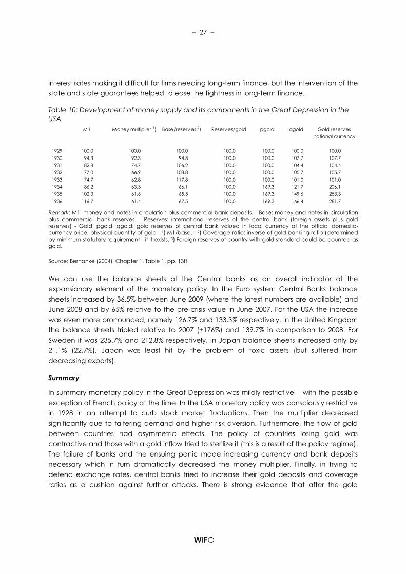
Table 10: Development of money supply and its components in the Great Depression in the
USA
M1 Money multiplier 1) Base/reserves 2) Reserves/gold pgold qgold Gold reserves
national currency
1929 100.0 100.0 100.0 100.0 100.0 100.0 100.0
1930 94.3 92.3 94.8 100.0 100.0 107.7 107.7
1931 82.8 74.7 106.2 100.0 100.0 104.4 104.4
1932 77.0 66.9 108.8 100.0 100.0 105.7 105.7
1933 74.7 62.8 117.8 100.0 100.0 101.0 101.0
1934 86.2 63.3 66.1 100.0 169.3 121.7 206.1
1935 102.3 61.6 65.5 100.0 169.3 149.6 253.3
1936 116.7 61.4 67.5 100.0 169.3 166.4 281.7
Remark: M1: money and notes in circulation plus commercial bank deposits. - Base: money and notes in circulation
plus commercial bank reserves. - Reserves: international reserves of the central bank (foreign assets plus gold
reserves) - Gold, pgold, qgold: gold reserves of central bank valued in local currency at the official domestic-
currency price, physical quantity of gold - 1) M1/base. - 2) Coverage ratio: inverse of gold banking ratio (determined
by minimum statutary requirement - if it exists. 3) Foreign reserves of country with gold standard could be counted as
gold.
Source: Bernanke (2004), Chapter 1, Table 1, pp. 13ff.
We can use the balance sheets of the Central banks as an overall indicator of the
expansionary element of the monetary policy. In the Euro system Central Banks balance
sheets increased by 36.5% between June 2009 (where the latest numbers are available) and
June 2008 and by 65% relative to the pre-crisis value in June 2007. For the USA the increase
was even more pronounced, namely 126.7% and 133.3% respectively. In the United Kingdom
the balance sheets tripled relative to 2007 (+176%) and 139.7% in comparison to 2008. For
Sweden it was 235.7% and 212.8% respectively. In Japan balance sheets increased only by
21.1% (22.7%), Japan was least hit by the problem of toxic assets (but suffered from
decreasing exports).
Summary
In summary monetary policy in the Great Depression was mildly restrictive with the possible
exception of French policy at the time. In the USA monetary policy was consciously restrictive
in 1928 in an attempt to curb stock market fluctuations. Then the multiplier decreased
significantly due to faltering demand and higher risk aversion. Furthermore, the flow of gold
between countries had asymmetric effects. The policy of countries losing gold was
contractive and those with a gold inflow tried to sterilize it (this is a result of the policy regime).
The failure of banks and the ensuing panic made increasing currency and bank deposits
necessary which in turn dramatically decreased the money multiplier. Finally, in trying to
defend exchange rates, central banks tried to increase their gold deposits and coverage
ratios as a cushion against further attacks. There is strong evidence that after the gold

– 28 –
standard was removed monetary policy became expansionary and became one element
necessary towards ending the Great Depression.20
Table 11: Fiscal balances 2006 to 2010: Per cent of GDP/Potential GDP
Note: Actual balances and liabilities are in per cent of nominal GDP. Underlying balances are in per cent of potential
GDP. The underlying primary balance is the underlying balance excluding the impact of the net debt interest
payments. - 1. Total OECD excludes Mexico and Turkey. - 2. Fiscal balances adjusted for the cycle and for one-offs.
Source: IMF, OECD Economic Outlook 85 database. http://dx.doi.org/10.1787/656585873210
Monetary policy behaved differently in the Current Crisis and it had less restrictions. Interest
rates were reduced to rates which were near to zero. No large region had a currency
problem or a gold standard. After interest rates reached zero, “quantitative easing” was
possible and was applied according to existing rules and where necessary even extending
them. A general consensus between countries and monetary and fiscal authorities allowed
for monetary easing thus making monetary policy effective in a “liquidity trap” situation.
Only countries (outside the Euro area) with currency problems had no option but to increase
the discount rate (and faced even more severe problems), but they obtained international
help from the IMF, the EU and the World Bank. Since there has been no deflation in 2009, real
and nominal interest rates did not differ very much. Short and long-term interest rates for
consumers and investors were higher than usual in recessions. Interbank lending did break
20 For an assessment of what caused an end to the Great Depression see Bordo (2008), Steindl (2008), Buchheim
(2003), Bernanke (2004), Temin (1976).

– 29 –
down. This together with the attempt by all banks to reduce leverage pushed up the interest
rates (much above the discount rate). But in most cases nominal and real interest rates
remained well below 10%, and then decreased rapidly as a result of policy measures such as
guarantees, fresh equity and quantitative easing (including the direct purchase of a wide
range of securities and commercial papers by the Fed and the ECB). The guaranteeing of
private deposits and even loans to large firms decreased the level of uncertainty and interest
rates.
Figure 10: Central Bank Discount Rates in Great Depression vs. Current Crisis
June 1931
May 2009
Source: Eichengreen - O’Rourke (2009).
Figure 11: Money Supplies in Great Depression vs. Current Crisis
2008
1930
Source: Eichengreen - O’Rourke (2009).

– 30 –
3.2 Fiscal Policy: balancing budgets vs. amplifying automatic stabilizers
Fiscal policy is not easy to describe without going into the details of federal, state and local
budget data and country details. Furthermore, government expenditure, as well as taxes, is
heavily influenced by the economic cycle, so that actual tax revenues will decline even if in
a recession taxes are raised and government expenditure is slashed (and vice versa). “Full
employment” budget data would reveal the effect of intentional policy measures as
opposed to surpluses or deficits generated by the business cycle. However these are rarely
available for the Great Depression (and not comparable to the Current Crisis). To our
knowledge, an analysis where actual budget figures as well as full employment figures are
calculated is available only for the USA (Brown, 1956).
US fiscal policy in the Great Depression
At all levels in the US government there was a budget surplus of about 1 bn $ in 1929.
Government expenditure increased in 1930 from 8.5 bn $ to 9.2 bn $ and remained stable in
1931. It then increased with the exception of a small dip in 1937 to 13.3 bn $ in 1939. Tax
revenues fell first slightly then massively to 6.4 bn $ in 1932, thus creating a large deficit (20% of
revenues) in 1932. The deficit was massive on the federal level; it was mitigated by surpluses
at the state and local level.
The “anti-cyclical” balances were not the results of an intentional policy. On the expenditure
side there was a “semi intentional part”, namely the enactment of large bonuses for veterans
by congress in 1931 (and 1936). Tax policy was highly pro cyclical thus reducing the
“automatic” decline due to decreasing business activity: tax rates were raised massively
across the board but notably in lower and middle income groups; earned tax credits were
slashed; corporate income tax was increased slightly; a gift tax was provided, and a broad
new list of excise taxes was levied. On the local level general sale taxes and excise taxation
were raised. Full employment budgets were heavily contractionary especially from 1933 to
1939 Brown, 1956, p. 868).21
The conclusion of Brown, “fiscal policy has been an unsuccessful recovery device in the
thirties- not because it did not work, but because it was not tried”, or by Hansen (1941)
“despite a fairly good showing made in the recovery of 1937, the fact that neither before nor
21 For a contrary view see Smithies (1946): ”fiscal policy did prove an effective and indeed the only effective means
of recovery”. This remark refers however to the period from 1938 onwards (and contrasts fiscal policy with
government control on wages and prices). In April 1939 President Roosevelt sent a document to the Congress
“Recommendations designed to stimulate further recovery”, ”that was the first outright recommendation….designed
to achieve recovery through fiscal policy” (Smithies, p. 16). “All the fiscal measures before had been trial and error,
increasing some taxes, financing public work programs, then curbing expenditures to balance the budget, then
enacting emergency budgets etc…. The first phases of the New Deal continued Hoover’s policy of cheap money,
home and farm relief programs, national industry recovery act, Labor Relations Act…”

– 31 –
since has the administration pursued a real positive expansionist program….federal
government engaged in salvaging program and not a program of positive expansion “.22
Fiscal policy: country evidence
Using standardized data on budget surpluses or deficits we see the following developments:
In the USA government (at the federal level) had surpluses in all the years between 1920 and
1929, all about 1% of GDP, with no pro or anti cyclical movements. This also holds true for 1929
and 1930. In 1931 a small deficit occurred (0.6% of GDP) followed by higher deficits in the
range of 4% to 5% and finally 7% in 1936 (these deficits may contain a “New Deal”
component). The deficit was reduced in 1937 and 1938 (to 3% and 1.4% respectively). In 1939
it was above 4% again.
In the Current Crisis the USA was one of the countries with a high deficit even before the crisis
started (2.9% in 2007). It suffered an increasing deficit in 2008 due to a deteriorating business
cycle. Early in 2009, one of the largest stimulus programs of any industrialized country (in
relation to GDP) was initiated by President Obama.
Germany had budget deficits in the twenties; the deficit was somewhat smaller in 1929 (1.8%)
and a little bit higher 1930 and 1931 (2.4% and 2.2% respectively). A surplus was created in
1933 and a balanced budget in 1934. Given that GDP decreased by 15% between 1929 and
1932 the data reveal energetic attempts to counteract the automatic stabilizers.23
As far as the Current Crisis is concerned, Germany had just managed a balanced budget
due to raising value added tax in 2008. Their stimulus package according to the OECD
calculation is 3.2% of GDP (2009/2010) with about an equal share spent over the two years
and in tax cuts as well as spending increases.
Austria managed a small surplus in 1929, followed by deficits of about 2% and 3% of GDP in
1930 and 1931. A balanced budget was reached in 1932 and then small deficits followed.
The deficit was reduced in 1936 and 1937 to 0.4% and 0.7%.
Austria had a nearly balanced budget in 2008, and then started early with significant stimulus
packages (including a tax reform in 2009). The stimulus packages are large if the tax reform is
included as well as measures for family support. According to the restrictive OECD definition
they are smaller.
France had a small surplus in 1928 and 1929, which it turned into a small deficit over the next
three years; large deficits are reported from 1933 to 1937 (and even larger ones in the
following years). The stimulus package 2009/10 according to OECD is rather small (0.7% of
22 The US budget was expansionary in 1936 due to a bill providing large veteran bonuses on the initiative of congress.
It was disliked but not vetoed by the President. The budget in 1937 was then specifically restrictive, due to the end of
the bonuses and the start of social security contributions. This contractionary effect is described by Romer (2009) as
premature elimination of public support for the economy, which led to another recession (which ended as the
budget became expansionary again).
23 Even acknowledging that the automatic stabilizers were much lower in the thirties (lower marginal tax rates, less
social expenditures).

– 32 –
GDP over two years), biased to the expenditure side. Budget deficits were high already at the
start of the crisis.
The United Kingdom had budget surpluses during every year preceding the Great Depression
and also during the ten following years (with a tiny deficit of 0.2% in 1932). It looks as if a
balanced budget had been the first priority. The crisis was milder in the United Kingdom than
in the USA, this is however not due to an expansion of fiscal policy.
Table 12: Comparison of two crises: budget deficit/surplus of central government
1920 to
1927 1928 1929 1930 1931 1932 1933 1934 1935 1936
1931-
1929
1931-
1936
1932-
1929 2007 2008 2009 2010 2010-2008
Average
Absolute
change
Austria -0.1 -0.7 0.2 -2.3 -3.1 -0.2 -2.7 -2.5 -1.7 -0.4 -3.3 2.7 -0.4 -0.7 -0.5 -4.3 -6.1 -5.6
Germany -8.6 -2.3 -1.8 -2.4 -2.2 -1.9 1.0 -0.4 2.2 -0.1 -0.2 -0.1 -3.9 -5.9 -5.8
Belgium -10.3 2.3 1.7 -1.9 -1.6 -3.9 -1.2 -2.2 -5.4 -4.6 -3.4 -2.9 -5.7 -0.3 -1.2 -4.6 -6.1 -4.9
Spain -1.6 1.5 1.1 0.8 -0.3 -0.8 -1.3 -1.8 -0.9 -1.5 0.3 -1.9 2.2 -3.8 -7.8 -8.7 -4.9
France -5.5 1.2 1.4 -1.5 -1.8 -1.7 -4.6 -3.8 -5.1 -6.9 -3.3 -5.1 -3.2 -2.7 -3.4 -6.6 -7.0 -3.6
Finland -1.6 -2.1 -0.8 -1.9 -2.3 -2.6 -1.6 -2.8 -3.8 -3.7 -1.5 -1.4 -1.8 5.2 4.1 -1.5 -2.8 -6.9
Sweden -1.7 -0.4 -0.6 -0.3 -0.4 -1.9 -4.0 -2.1 -2.5 -2.2 0.2 -1.8 -1.3 3.8 2.5 -3.3 -4.5 -7.0
United Kingdom 1.8 1.8 0.8 1.0 0.8 -0.2 1.0 0.5 0.4 0.2 0.0 -0.6 -0.9 -2.7 -5.5 -12.8 -14.0 -8.5
USA 0.9 1.0 0.7 0.8 -0.6 -4.7 -4.6 -5.5 -3.8 -7.0 -1.3 -6.4 -5.4 -2.9 -5.9 -12.1 -14.2 -8.3
Japan 8.0 4.5 3.9 2.4 3.1 0.1 -0.5 0.7 1.1 2.4 -0.8 -0.7 -3.8 -2.5 -2.7 -6.7 -8.7 -6.0
"World" -0.5 0.8 0.6 0.1 -0.5 -2.5 -2.3 -2.7 -2.2 -3.5 -1.1 -3.0 -3.1 -1.9 -3.8 -8.7 -10.3 -6.5
Unweighted average over countries -1.9 0.7 0.7 -0.5 -0.8 -1.8 -1.8 -2.2 -2.4 -2.8 -1.5 -1.9 -2.5 -0.1 -1.7 -6.4 -7.8 -6.2
Standard deviation 4.2 1.7 1.2 1.4 1.2 1.6 2.2 1.7 2.0 2.9 1.4 3.1 2.0 2.9 3.4 3.9 4.0 1.6
Coefficient of variation -2.272 2.479 1.746 -2.744 -1.452 -0.875 -1.173 -0.797 -0.844 -1.039 -0.934 -1.579 -0.835 -36.872 -2.085 -0.616 -0.509 -0.266
Current crisis (2007ff)
Annual data
Great Depression (1932)
Absolute changeAnnual data
Remark: "World": Weighted by GDP.
Sources: USA: 1900-1969: WIFO-calculations using Mitchell 1999 (Central Government), 1970-2010: OECD (General
Government, net lending). – Japan: 1900-1954: Bordo using Mitchell, 1955-1969: IFS Yearbook 1989 (all: Central
Government), 1970-2010: OECD (General Government). - Germany: 1900-1951: Bordo using Mitchell (1991), 1922-
1923, 1935-1949 not available, 1952-1969 IFS Yearbook 1998, 1970-2010: OECD (General Government). - France: 1900-
1949: Bordo using Mitchell (1992), 1950-1969: IFS Yearbook 1998 (all: Central Government), 1970-2010: OECD (General
Government). - Italy: 1900-1949: Bordo using Mitchell (1992), 1950-1969 IFS Yearbook 1998, 1970-2010: OECD (General
Government). - Spain: 1900-1969: Bordo using Mitchell (1992), 1970-2010: OECD (General Government). -
Netherlands: 1900-1949: Bordo using Mitchell (1992), 1950-1969 IFS Yearbook 1998, 1970-2010: OECD (General
Government). - Belgium: 1920-1969: Bordo using Mitchell, 1970-2010: OECD (General Government). - Portugal: 1900-
1969 Bordo using Mitchell (1992), 1970-2010: OECD (General Government). - Finland: 1900-1969: Bordo using Mitchell
(1992), 1970-2010: OECD (General Government). - Greece: 1900-1969 Bordo, 1970-2010: OECD (General
Government). - United Kingdom: 1900-1969: WIFO-calculations using Mitchell 1999, 1970-2010: OECD (General
Government). - Ireland: 1970-2010: OECD (General Government). -Sweden: 1900-1949: Bordo using Mitchell(1992),
1950-1969: IFS Yearbook 1998, 1970-2010: OECD (General Government). - Denmark: 1900-1949: Bordo using
Mitchell(1992), 1950-1970: IFS Yearbook 1998, 1971-2008: OECD (General Government). - Switzerland: 1900-1989:
Bordo using Mitchell and IFS Yearbook 1998, 1990-2008: OECD (General Government). - Austria: 1924-1937: WIFO-
calculations, Bundesrechungsabschluss and League of Nations (1927-1934): expenditures including redemption to
loans (Central Government); 1938-1945: not available; 1946-1953: WIFO-calculations, Bundesrechungsabschluss;
expenditures including redemption to loans; 1954-1969: WIFO-calculations, Bundesrechnungsabschluss: expenditures
exclude redemption to loans (net lending in % GDP), Central Government; 1970-2010: OECD (General Government).
- Germany, France, Japan, USA 2008, 2009 Eurostat, Spring 2009.
At the start of the Current Crisis the United Kingdom had the highest deficit of Western
Europe; it suffered a further deterioration by the crisis. OECD measures the stimulus package
to 1.9% of GDP, mainly via a tax reduction in 2009.

– 33 –
Figure 13: Government Budget Surpluses in the Great Depression vs. Current Crisis
1929
2010 world2009
advanced
countries
Source: Eichengreen - O’Rourke (2009).
Sweden had small deficits in the run up to the Great Depression. In 1933 and the years that
followed the deficit was somewhat higher without any policy change. Despite being neutral
in the war they had double-digit deficits during the war.
Sweden had a budget surplus of 4% at the beginning of the Current Crisis. It enacted a strong
stimulus package (3.3% of GDP equally divided between tax reductions and expenditure)
where “green” measures are fostered and the already high research expenditure is further
supported. It is one of the few countries using stimulus packages to improve future projects.
Italy is the only country which boosted demand early; deficits rose to 5% in 1932 and stayed
at that level up until the war.
Fiscal policy and stimulus packages: the overall picture in 2008/09
Fiscal policy was intensively used in the Current Crisis to mitigate the downturn by providing
stimulus packages, recapitalizing banks and allowing automatic stabilizers to work. This last
element seems to be largest (and multipliers are higher in Europe). Automatic stabilizers have
no implementation lag (which proved significant again in this crisis). Very few countries had
surpluses in their total fiscal balances at the start of the crisis. Japan and specifically the US
started with high deficits (2.5%, 2.7% respectively). The Euro area had a small deficit as
compared to previous years (2007: 0.7%, but deficits were high in the United Kingdom and
France).
– 34 –
All countries allowed the automatic stabilizers to work in 2008 and 2009; the OECD estimates
that the cumulative effect of the automatic stabilizers over 2009 and 2010 made up for half of
the “deterioration of fiscal balances” (OECD, 2009, p. 56). The remaining half is made up of
“structural measures” which can be further subdivided into discretionary measures in
response to the financial crisis (making up one fifth); and a larger part from the loss of
exceptional revenues related to the asset price boom and the buoyant growth in
construction and financial service (OECD, 2009, p. 56). Fiscal stances as measured by
structural balances (adjusted for cycles and one-offs) are expansionary in 2009 and 2010. In
Germany and Italy, as well as in the Euro area as a whole, fiscal stance is expected to be
more expansionary in 2010 than in 2009 (the same holds for the USA).
Estimating the size and timing of a stimulus pattern is not an easy task. Different assessments
are provided by the OECD, the EU Commission and Saha Weizsäcker (2009)24. The OECD
assesses them to be about 4% of GDP for the years 2008 to 2010 (weighted average,
unweighted 1.7%), using a rather restrictive definition of stimulus packages. The stimulus is
concentrated in 2009, the second largest part will have an effect in 2010. The division
between spending and tax cuts is about equal. The discretionary stimulus packages are
highest in the USA, Australia, Korea, and in small European countries. Ireland, Hungary and
Iceland could not afford an expansionary policy due to budget or currency problems.
While the extent and impact of fiscal packages is open to further investigation, the overall
picture is clear. This time almost no countries tried to counteract the automatic stabilizers by
enforcing a balanced budget. All countries tried to stimulate demand using fiscal measures,
some with more room to maneuver than others due to past surpluses or a strong currency (or
Euro membership)25 and some with more courage than others (the Non-European countries).
This discretionary part of the fiscal policy is the part of the fiscal effects, one fifth according to
a somewhat restrictive definition in OECD (2009).
In almost all countries the public deficits are running at over three percent26 (which was set as
the upper limit by the EU). In the USA and in Great Britain public deficits are running into
double-digit figures.27 The actual deficit in 2009 is predicted to be 10% in the USA, 8% in Japan
and 6% in the Euro area (see table 11).
24 The size of the stimulus packages is calculated differently depending i) on whether the scope of the stimulus is
limited to discretionary measures, ii) on which policies would have been implemented had there not been a crisis
(i.e. which other policy measures are included in the stimulus packages) and iii) on whether or not the effects of any
stimulus are calculated for one year or more. There are many extensive international comparisons by the OECD
(Interim Report 2009), by the European Commission (2009) and by Saha Weizsäcker (2009). Estimates by the
European commission and by Saha - Weizsäcker are higher than those of the OECD, especially for European
countries.
25 In Hungary, Iceland, Ireland and the Baltic States there were in fact negative stimuli as a result of the very high
deficits of the state.
26 The EU Commission reckons that in 2009 12 and in 2010 17 EU-countries will break the rules on deficit limits. The goal
of the ensuing excessive deficit procedures should be to work on a medium term path of adjustment (while the
countries are being encouraged to increase short term deficits).
27 In some countries there are also short term purchasing incentives (scrapping premiums or reduction of VAT).
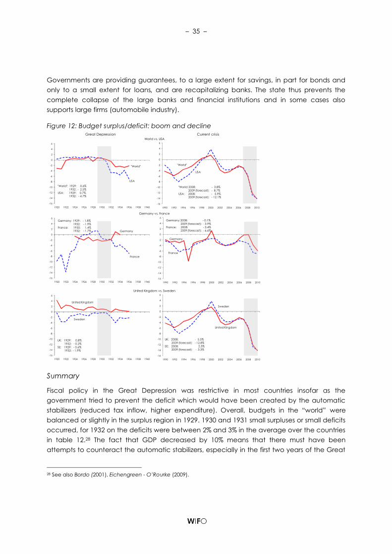
– 35 –
Governments are providing guarantees, to a large extent for savings, in part for bonds and
only to a small extent for loans and are recapitalizing banks. The state thus prevents the
complete collapse of the large banks and financial institutions and in some cases also
supports large firms (automobile industry).
Figure 12: Budget surplus/deficit: boom and decline
1408.89715
1408.89715
1408.89715
Great Depression Current crisis
United Kingdom vs. Sweden
Germany vs. France
World vs. USA
-16
-14
-12
-10
-8
-6
-4
-2
0
2
4
6
1990 1992 1994 1996 1998 2000 2002 2004 2006 2008 2010
UK: 2008: - 5.5%
2009 (forecast): - 12.8%
SE: 2008: 2.5%2009 (forecast): - 3.3%
Sweden
United Kingdom
-16
-14
-12
-10
-8
-6
-4
-2
0
2
4
6
1920 1922 1924 1926 1928 1930 1932 1934 1936 1938 1940
UK: 1929: 0.8%
1932: - 0.2%
SE: 1929: - 0.6%1932: - 1.9%
United Kingdom
Sweden
-16
-14
-12
-10
-8
-6
-4
-2
0
2
4
6
1990 1992 1994 1996 1998 2000 2002 2004 2006 2008 2010
France
Germany
Germany: 2008: - 0.1%
2009 (forecast): - 3.9%
France: 2008: - 3.4%2009 (forecast): - 6.6%
-16
-14
-12
-10
-8
-6
-4
-2
0
2
4
6
1920 1922 1924 1926 1928 1930 1932 1934 1936 1938 1940
Germany
Germany: 1929: - 1.8%
1932: - 1.9%
France: 1930: 1.4%1932: - 1.7%
France
-16
-14
-12
-10
-8
-6
-4
-2
0
2
4
6
1990 1992 1994 1996 1998 2000 2002 2004 2006 2008 2010
"World: 2008: - 3.8%
2009 (forecast): - 8.7%
USA: 2008: - 5.9%2009 (forecast): - 12.1%
USA
"World"
-16
-14
-12
-10
-8
-6
-4
-2
0
2
4
6
1920 1922 1924 1926 1928 1930 1932 1934 1936 1938 1940
"World": 1929: 0.6%
1932: - 2.5%
USA: 1929: 0.7%1932: - 4.7%
"World"
USA
Summary
Fiscal policy in the Great Depression was restrictive in most countries insofar as the
government tried to prevent the deficit which would have been created by the automatic
stabilizers (reduced tax inflow, higher expenditure). Overall, budgets in the “world” were
balanced or slightly in the surplus region in 1929. 1930 and 1931 small surpluses or small deficits
occurred, for 1932 on the deficits were between 2% and 3% in the average over the countries
in table 12.28 The fact that GDP decreased by 10% means that there must have been
attempts to counteract the automatic stabilizers, especially in the first two years of the Great
28 See also Bordo (2001), Eichengreen - O’Rourke (2009).

– 36 –
Depression. On the other hand there had been attempts to target expenditure quite
specifically (relief work, veteran bonuses etc). Later during the Great Depression there were
explicit measures to combat unemployment through public work (Big Deal in the US,
preparation for the war in Germany). From 1932 to 1936 budget deficits amounted to 4% of
GDP in many countries (USA, France, Italy, and Netherlands). Others like the United Kingdom
and Japan tried again, and with success, to balance their budgets. The literature is
undecided as to what was essential in bringing an end to the Great Depression, but
alongside an expansionary monetary policy, the more active approach of some
governments will have helped as will the preparations for war later on.
In the Current Crisis fiscal policy adopted an expansionary stance in almost all countries. The
larger proportion of increased budget deficits is the result of reduced tax revenues and
increased government spending ("automatic stabilizers"). In addition fiscal stimulus packages
were created in which there were tax cuts and increases in expenditure, including
expenditure recapitalizing the banks. The cuts in taxes stretched from income tax to VAT.
Undisputed is that the packages in the USA were bigger than in Europe (OECD: 5.6% on
average 2008 to 2010, compared with 0.9% in the EU). In Australia, Canada, New Zealand,
Korea and China the packages were also very large.
3.3 Labor market and employment policy
The unemployment and even more the employment data demonstrate that the difference
between the two crises has been dramatic, even if we extend the horizon of the Current Crisis
to 2010 and 2011 (using predictions). We know from past crises that the turning point for
unemployment can be two years later than for production (Reinhardt Rogoff, 2009).
The Great Depression
One fourth of the labor force was unemployed in the Great Depression in the USA, Germany,
and Austria (15% in the United Kingdom). At that time the labor force was between one third
(USA) and one half of the persons employed today in most other countries (again with the
United Kingdom at the lower end).29 GDP is between eightfold and tenfold today as
compared to 1929, and even a dramatic decrease of 10% in the industrialized countries in
the Current Crisis which will not occur according to today’s predictions) would not destroy
the picture of a much richer society (at the beginning and hopefully at the end of the crisis).
Social security systems will furthermore prevent poverty (at least absolute poverty in
developed countries).
However, unemployment is the one variable where we really have no way of knowing how
the story might end, even if the decrease in production is leveling off (as it seems to do in
September 2009). Unemployment figures will increase in the next one to one and a half years,
29 The population has been growing since the thirties but much less than employment, showing increasing
employment ratios.

– 37 –
if not for longer surpassing 10% in the USA and eventually also in the EU. For most countries an
economic growth of 1-1½% is not sufficient to decrease unemployment.
The USA had a severe crisis in 1921 in which unemployment rose from 1.4% to 11.7% within two
years, the lowest rate was then reached in 1926 with 1.8%. Thus the pre-crisis period had been
bumpy and the data show the cooling off of the real economy well before 1929.
Unemployment then rose from 3.2% in 1929 to 24.9% in 1933, it then declined a little, and then
had an often cited one year increase in 1938 (see fiscal policy chapter). The New Deal,
expansionary monetary policy and/or the preparation for the war eliminated unemployment
between 1941 and 1945.
The development in the United Kingdom was similar to that of the USA as regards the crisis of
1920. The unemployment rate at the start of the Great Depression was much higher (7.3%),
but increased less than in the USA, reaching a maximum of 15.6% in 1932.
Germany and Austria had no crisis in 1921/22, indeed their lowest unemployment rate were
1.5% and 1.1% in 1922 and 1921 resp. They did have hyper inflation and then the
unemployment rate rocketed sky high until 1926 (to 18% and 13% respectively).
Unemployment showed a falling trend up until 1929 (at levels of 9.3% and 12.2%). Fiscal policy
became more expansionary from 1932 onwards initially without any military focus. Hitler’s
policy slashed unemployment to less than 5% in 1937 in Germany (then to 2% in 1938). In
Austria unemployment decreased slightly up until 1937, than it was halved by 1938 and then
eliminated.30
Employment figures give a similar picture: a very strong decline in the USA and in the United
Kingdom in 1921, where the one year decline was as large in absolute figures as in the first
year of the Great Depression. Employment loss in the Great Depression was larger in the USA
(9 million out of 47.6 million), and very small in the United Kingdom (0.7 million out of 19.5
million). Previous levels were regained in 1941 in the USA. Employment loss was similar in
Germany and Austria (-5.1%, 0.3% between 1929 and 1932 respectively).
Current Crisis
In the Current Crisis unemployment had reached its lowest level of between 4% and 5% in the
USA and in the United Kingdom, well before the crisis started (in 2006 and 2004 resp.). It
increased during the crisis rapidly specifically in the USA, from 4.6% in 2007 to 9% for 2009.
Germany has a somewhat different pattern as it experienced a double-digit unemployment
rate in 2005 (11%). This decreased through labor market reform and export led growth in 2008
to 7.5%, and up to now a steep increase has been prevented.
30 There is an alternative view that recovery was already on course before Hitler’s program could be have any affect
(Buchheim, 2003).

– 38 –
Employment policy: from relief programs to short working time subsidies
As far as economic policy is concerned the differences in macroeconomic policy are
described in the chapter on fiscal and monetary policy. As far as labor market policy itself is
concerned we concentrate on the USA, due to the focus of the international literature. For
other countries see Eichengreen Hatton (1988). The USA tried to mitigate unemployment
early through intensive work relief programs (in which the government employed people at
low wages). Starting in 1930 0.6%, and then in 1935 a maximum of 5.9% of unemployment was
“parted” in relief programs: the unemployment rate including relief program workers was
20.1% in 1935, and 14.2% without (Margo, 1993, p. 42). Another important feature of labor
market policy was that firms did not cut wages. Indeed real wages were increasing sharply
during the recession e.g. by 20% between 1929 and 1931. Then came a phase of ups and
downs, but with a trend of 30% higher real wages in 1939 as compared to 1929 (Margo, 1993,
Bernanke, 2004, etc). This trend of rising real wages is blamed for the length of the recession
according to the macroeconomics of the time. There had been a lot of variation in working
times, which mitigated costs for firms and which may have encompassed an element of
lowering wages not reflected in the statistics. There are several explanations as to why real
wages increased despite the slump. The first one is the stickiness of nominal wages which, due
to falling prices, increased in real terms. Other authors cite an echo effect from the recession
in 1921, in which wages had been cut and the crisis worsened. Furthermore, reference is
given to a social norm, that firms should not decrease wages in recession. Finally, the
concept of efficiency wages could be used. Firms did not like to cut wages since this lowered
motivation and productivity.
A macroeconomic policy in the Keynesian tradition was not applied and there would
have been no channel at that time. Roosevelt’s New Legislation, the National Industry
Recovery Act of 1933, established guidelines that raised nominal wages and prices and
encouraged higher levels of employment through reducing the working week. Part of the
legislation was declared unconstitutional in May 1935; its effect had been investigated by
Weinstein (1980) and criticized by Temin (1976) for increasing the persistency of
unemployment.
In the Current Crisis in many countries labor market policies have been used to dampen the
effects on employment of the declining economic activity. Programs have been started to
support shorter working time in specifically hard-hit firms (“Kurzarbeitsprogramme”). This is
likely to be the reason why e.g. in Germany and Austria the increase in unemployment and
the decline in employment compared with the decline in GDP is actually less than in the USA.
A less pronounced decline in employment in turn stabilizes GDP via consumption. The impact
of the crisis is also reduced if the mismatch between the supply and demand of qualifications
is minimized and if regional and job mobility is increased. In many countries, before the crisis,
the job market was close to full employment, especially for qualified people, and firms were
limited in their ability to expand production. Indeed even during the crisis there are some job
vacancies where there is a lack of appropriately qualified people.

– 39 –
A general shortening of work time has not been considered (the same holds for large early
retirement programs), specifically since in most industrialized European countries the
population of working age is predicted to shrink in the next years due to an ageing
population. Efforts to re-train workers is in theory high on the agenda since unemployment is
very different across qualifications and sectors, but it proved difficult to implement in a crisis
which came at such a high speed.
3.4 Protectionism
As it is well known one of the policy changes in the Great Depression was to shelter one’s own
economy from the negative impacts of the world depression. A specific form of protectionism
cited over and over in the literature was the SmootHawley Tariff Act (1930), in which
tariffs on imports were raised. In parallel, tariffs and duties were also increased in many other
countries. The average tariff rate across the fourteen countries rose by 12.7% during the Great
Depression (Newell Symons, 1988).
It is difficult to find general indicators for protectionism. One could use the customs inflow as a
percent of GDP. This indicator was flat for the USA between 1925 and 1928, but increased
somewhat in 1929. There was no specific pattern in the following years, but then a steep
increase in 1936.
In European countries the level of custom inflows relative to GDP was higher. The receipts
strongly increased already in the build-up period (specifically in France, Germany and
Austria). Receipts relative to GDP were flat in the United Kingdom and decreased a little bit in
Sweden. From 1929 to 1935 they exploded in the United Kingdom and France. The increase
was not so pronounced in Germany and tariffs relative to GDP decreased in Austria starting in
1931. In general the picture indicates more restrictive policies in the European countries
relative to the USA with the exception of Sweden.
Thus protectionism if measured correctly by this indicator did not start the Great
Depression, but played a role in prolonging and deepening it. It seems to have been applied
more in Europe than in the USA, where the Smoot Hawley Tariff Act is so prominently
discussed.
This time international coordination meetings (G20, EU Commission, IMF, OECD) discuss and
monitor the danger of protectionism (apart from WTO). “Buy National Clauses” were
clandestinely or openly put into many stimulus programs, usually arousing international
protest. They were consequently mitigated, albeit not totally abandoned. New export duties
came into existence even before the crisis (to limit the outflow of resources or food in the
period of scarcity before the crisis started), but these have up to now been limited. Rising
tensions could however come up if the crisis continues and problems arise if there are large
imbalances (see the conflict about tires between the USA and China in September 2010 and
the Chinese threats of retaliation).

– 40 –
Table 13: Crises vs. Periphery - GDP
1929 1930 1931 1932 1932/1929 2007 2008 2009 2010 2010/2007
USA 6.1 -8.9 -7.7 -13.2 -27.0 2.1 0.4 -2.8 1.9 -0.5
Euro-zone 2.7 -1.6 -5.2 -3.1 -9.6 2.7 0.6 -4.4 0.2 -3.7
Germany -0.4 -1.4 -7.6 -7.5 -15.8 2.6 1.0 -5.8 0.6 -4.4
France 6.8 -2.9 -6.0 -6.5 -14.7 2.3 0.3 -2.2 0.6 -1.3
United Kingdom 2.9 -0.7 -5.1 0.8 -5.1 2.6 0.7 -4.7 0.3 -3.7
Japan 3.1 -7.3 0.8 8.4 1.3 7.3 5.6 -6.1 1.5 0.7
Eastern Europe 1.0 -1.9 -3.4 -5.6 -10.5 7.3 5.6 -6.1 1.5 0.7
Russian Federation 2.8 5.8 1.9 -1.1 6.7 8.1 5.9 -9.6 3.3 -1.2
Ukraine 7.3 2.1 -7.8 1.6 -4.4
Brazil 0.2 -6.0 -2.2 3.5 -4.9 5.4 5.1 -1.2 3.8 7.8
South-Korea -4.8 -4.9 1.3 0.9 -2.8 5.1 2.2 -1.4 3.3 4.1
China 1.3 1.0 3.2 5.6 13.0 8.9 8.1 8.6 27.9
India 4.2 0.7 -0.7 1.1 1.2 9.0 7.5 5.5 6.9 21.2
Indonesia 2.8 0.7 -7.5 -1.2 -7.9 6.3 6.1 2.6 4.0 13.3
World 3.7 -1.9 -4.2 -4.0 -9.8 3.8 1.6 -2.5 2.1 1.2
Unweighted average over countries 2.0 -2.2 -2.2 -0.7 -4.8 6.7 4.5 -2.1 3.3 6.0
Unweighted average over periphery countries 1.0 -0.6 -1.4 0.1 -1.8 7.7 5.4 -1.2 4.1 8.7
Standard deviation 3.1 4.5 3.6 5.8 9.9 3.0 2.8 5.6 2.5 10.6
Coefficient of variation 1.527 -2.072 -1.687 -8.192 -2.057 0.446 0.613 -2.664 0.756 1.771
Current crisis (2007ff)Great Depression (1932)
Remark: “Periphery countries”: all countries in table but USA, Euro-zone and Japan.
Source: individual countries: Groningen (1900-2006), Oxford Economic Forecasting Ltd. (2007-2010, real data).
4. Conclusion, summary, caveats
(1) The goal of this paper is to compare the Great Depression of the last century with the
Current Crisis, which started in 2007 and spread across the world at increasing speed in 2009.
The comparison does not focus on the causes of either crises or on any similarities or
differences (since this is done in other papers). Rather we focus on and compare the depth
of the crises and the policy reaction. Both these aspects make it necessary to analyze the
build-up period to the crises and this is done mainly by looking for stylized facts. This serves to
enrich the search for the causes and consequences of the crises. The analysis and
comparison of the two crises should also help to assess the probability of its recurrence. The
analysis has to be seen as an early or even possibly premature attempt, since even though as
of September 2009, the fall in production seems to be leveling off, we cannot be sure of this.
What we do know from economics and from history is that the crisis will have a longer
negative effect on the labor market, and will have a lasting impact on budgets, leverage
ratios, risk taking and the behavior of firms, consumers, and governments in general. The
negative social and economic consequences will be long lasting, as will be hopefully the
– 41 –
lessons learned by the economic and political system and the impetus for reforms
(international coordination, regulation, longer-term goals etc.).
(2) The depth of the two crises, if the current one levels off in 2009, will have been very
different. The difference is largest for real GDP, and less pronounced for exports and for
industrial production. It is also very different for the stock market, even though this is a market
where the ups and downs are likely to continue and the current rally may not last. The largest
difference is seen in employment and unemployment (the level of and changes in both). In
addition the starting position regarding income, poverty, social security net and income
differences (between rich and poor) could not be larger. The income level (price adjusted
GDP) at the start of the two crises also differ on a scale of 1 : 8 or 1: 10.
(3) The loss of GDP (real at PPP) between 1929 and 1932 reached between 15% and 25%
in the countries most hit by the crisis, and about 10% for the average of industrialized
countries (for estimates of world GDP). It took six years to regain the pre-crisis level, with some
countries not managing this before the start of WWII (USA, France, Spain 1951 and Austria).
In the Current Crisis world GDP is forecast to shrink between 1% and 2% in only one year
(2009). World economic growth was higher (than the one year loss) in the year before the
Current Crisis (2008) and world GDP currently is forecast to surpass the old maximum in 2010.
The decline in GDP in 2009 is expected to be larger for the USA (as compared to the decline
of world GDP) and even larger for the Euro-area and for the EU-27. Amongst the large
countries GDP loss in 2008/2009 is forecast to be highest in Japan and in Germany, both,
however, reported growth as soon as in 2Q/2009. The fall is still larger in Ireland, Finland, and
Sweden and in some new EU member countries. Outside the EU, Russia, Ukraine and Turkey
are especially hit, as are some Asian countries. Output is expected to grow even in 2009 in
Poland, China and India, in the latter countries at a high and increasing rate (after diminished
growth in late 2008). In the Great Depression the drop in GDP was largest in the USA (-27%
between 1929 and 1932), followed by Germany, Austria, and France, with the United
Kingdom facing a small recession. Denmark and Japan continued to enjoy positive growth
between 1929 and 1932.
The extent of both crises is not fully reflected in annual data. If we use quarterly data, the loss
for the USA and the EU-area in the Current Crisis increases to 3.9% and that of Germany to 7%.
Both rates are still definitely lower than the loss in the Great Depression (which using quarterly
data would also show higher rates of maximum decline).
(4) In both crises economic growth was buoyant in the eight years preceding the crisis.
This growth dynamic was more stable in the Current Crisis, despite of the dot.com crisis, which
proved with hindsight to only be a growth recession. Some countries, notably the USA, had
had a severe recession at the start of the twenties. Austria and Germany suffered from
hyperinflation in the 1920s. At the start of the recession in 1929 inflation was moderate. There
were no shortages of raw material, energy, or food, and there was even a little underlying
deflationary tendency (in the United Kingdom, USA), overcapacities were reported in
different industries in the USA, several European countries had low outputs relative to pre-WWI

– 42 –
GDP. Cyclical growth had peaked before, although stock prices continued to rise,
expectations were more optimistic than the actual facts supported. Leading indicators
(similar to the Harvard Barometer) predicted a depression as early in 1928.31
At the start of the Current Crisis, shortages of raw material, energy, and food existed and
inflation was increasing to a level not known before in the period of “great moderation”. This
was the label used to characterize the period between 1990 and 2007 for combining solid
growth with low inflation. World economic growth reached 20% over five years (2002 to 2007),
with higher growth rates in Asia, the BRICS, and Eastern Europe contributing to the shortage
mentioned (and stimulated speculation which pushed prices to above equilibrium values).
(5) As far as manufacturing is concerned the decline in the Current Crisis is also smaller
than in the Great Depression, but the difference is smaller than for GDP. A composite
indicator of “world” industrial production, weighted by GDP, decreased by 30% in the Great
Depression, and only by 19% in the Current Crisis, as measured by annual rates (and assuming
the lowest value is reached in 2009). This is specifically true for the USA and Germany. In
Japan, Spain, UK, Finland and Sweden the fall in production has been steeper in this crisis.
Cross country variation in the rates of decline is much less in the Current Crisis. This is a
consequence of globalizing industrial markets.
(6) The decline of exports (and world trade, in nominal figures) is also smaller in the
Current Crisis. The difference between the decline in exports falls between the larger
difference in GDP loss and the smaller difference in manufacturing production. The decline in
exports for the USA in the Current Crisis is much smaller (as compared to the Great Depression
but also to other countries). The decline in the Current Crisis is very similar across countries and
had been very strong between September 2008 and February 2009 (taking monthly data by
Eichengreen - O’Rourke, 2009), stronger than during the Great Depression.
(7) Unemployment during the Great Depression jumped from 3% in 1929 to 15% in 1932,
reaching 25% in Austria and the USA, and 30% in Germany (16% in the United Kingdom). In the
Current Crisis it started with levels between 5% and 8% in most industrialized countries, and the
unemployment rate is bound to reach the 10% mark in the EU and the USA. We are definitely
not in a position at the moment to know the end of the story, since unemployment rates
continue to increase well after the production ceases to decline and starts to grow.
Decreasing unemployment would need growth rates, currently not predicted in most
countries (at least for 2010).
Employment decreased by 16% on average across countries in the Great Depression (-14% in
the USA, -29% in Germany). Employment loss is forecast to be 2.6% in the EU in 2009 and 3.5%
in the USA.
(8) Switching to quarterly or monthly data (wherever possible) and looking at the speed
of the decline shows that for manufacturing, exports and stock prices there are several
31 “The picture resembles the typical constellation at the beginning of a depression“, (WIFO Monthly Bulletin
(Monatsberichte), December 1928, p. 188. Indicators used referred to money market, stocks and goods.

– 43 –
months or quarters where the speed of decline between the Great Depression and the
Current Crisis had been similar or even larger in the Current Crisis. For the stock markets the
decline was at first smaller in the lingering phase of the Current Crisis, then between
August/September 2008 and February/March 2009 much steeper (if we include the last
rebound of stock markets since March 2009). The decline continued beyond the first 18
months in the Great Depression, while this time stock prices started to rebound in March 2009
(by more than one third up to August). Industrial production declined faster in this crisis from
August to October 2008. The same is true for world trade between September 2008 and
February 2009.
The similarity of the speed of decline, even if only over a few months and with regards to the
most volatile indicators, demonstrates that the potential for a much steeper recession existed
in the Current Crisis. It furthermore indicates very strongly that the difference in economic
policy between the Great Depression and the Current Crisis mattered. Additionally two
institutional factors helped slow any decline: manufacturing is today only a much smaller part
of the economy (service sector and public sector are larger), and secondly some countries
on the “periphery” (i.e. countries which do not lead in per capita income and which were
not at the epicenter of the crisis), did not suffer that much from the problems of the
industrialized countries, some countries had reserves to stabilize their economies, others
received assistance from the IMF. On the other hand financial globalization and intensified
trade relations could have had the potential to create a longer and much synchronized
global crisis.
(9) Two specific features of the Great Depression were its length and that it occurred in
several stages. It started with the stock market crash (October 1929) hitting economies at the
downturn of a business cycle. This was followed by a breakdown of world trade, then by a
wave of bank runs and bank failures. Economic policy reacted lenient, indecisive and late.
Monetary policy was restricted by the gold standard and was applied in an asymmetric,
restrictive way. The fiscal policy tried to balance budgets and prevented automatic stabilizers
from working. Competitive devaluations, rising taxes and tariffs, and finally a premature
reduction of deficits (in the USA in 1937) increased the length of the Great Depression. It was
the length, not the initial speed, of the Great Depression, which made the cumulative decline
in output and employment that large. This time the speed in the beginning was high,
mitigated by some new economic characteristics and by decisive and at least partly
coordinated policy measures.
(10) It is not easy to describe the policy reaction from data alone. Specifically data
demonstrating the role of purposive policy (as opposed to changes in fiscal balances or
changes in money supply driven by a downturn) are rarely available over the whole period
and monetary as well as fiscal multipliers are very different between then and now. So we
have partly to rely on assessments in the literature, qualitative reports and on specific data
not comparable across countries and over time.
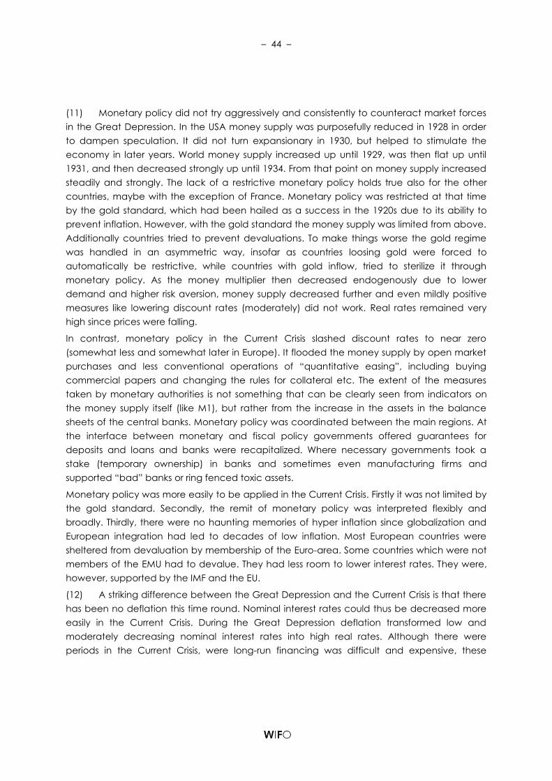
– 44 –
(11) Monetary policy did not try aggressively and consistently to counteract market forces
in the Great Depression. In the USA money supply was purposefully reduced in 1928 in order
to dampen speculation. It did not turn expansionary in 1930, but helped to stimulate the
economy in later years. World money supply increased up until 1929, was then flat up until
1931, and then decreased strongly up until 1934. From that point on money supply increased
steadily and strongly. The lack of a restrictive monetary policy holds true also for the other
countries, maybe with the exception of France. Monetary policy was restricted at that time
by the gold standard, which had been hailed as a success in the 1920s due to its ability to
prevent inflation. However, with the gold standard the money supply was limited from above.
Additionally countries tried to prevent devaluations. To make things worse the gold regime
was handled in an asymmetric way, insofar as countries loosing gold were forced to
automatically be restrictive, while countries with gold inflow, tried to sterilize it through
monetary policy. As the money multiplier then decreased endogenously due to lower
demand and higher risk aversion, money supply decreased further and even mildly positive
measures like lowering discount rates (moderately) did not work. Real rates remained very
high since prices were falling.
In contrast, monetary policy in the Current Crisis slashed discount rates to near zero
(somewhat less and somewhat later in Europe). It flooded the money supply by open market
purchases and less conventional operations of “quantitative easing”, including buying
commercial papers and changing the rules for collateral etc. The extent of the measures
taken by monetary authorities is not something that can be clearly seen from indicators on
the money supply itself (like M1), but rather from the increase in the assets in the balance
sheets of the central banks. Monetary policy was coordinated between the main regions. At
the interface between monetary and fiscal policy governments offered guarantees for
deposits and loans and banks were recapitalized. Where necessary governments took a
stake (temporary ownership) in banks and sometimes even manufacturing firms and
supported “bad” banks or ring fenced toxic assets.
Monetary policy was more easily to be applied in the Current Crisis. Firstly it was not limited by
the gold standard. Secondly, the remit of monetary policy was interpreted flexibly and
broadly. Thirdly, there were no haunting memories of hyper inflation since globalization and
European integration had led to decades of low inflation. Most European countries were
sheltered from devaluation by membership of the Euro-area. Some countries which were not
members of the EMU had to devalue. They had less room to lower interest rates. They were,
however, supported by the IMF and the EU.
(12) A striking difference between the Great Depression and the Current Crisis is that there
has been no deflation this time round. Nominal interest rates could thus be decreased more
easily in the Current Crisis. During the Great Depression deflation transformed low and
moderately decreasing nominal interest rates into high real rates. Although there were
periods in the Current Crisis, were long-run financing was difficult and expensive, these

– 45 –
periods were shortened by monetary policy and complementary guarantees. Support
measures by governments and international organizations were also provided.
(13) Fiscal policy is difficult to describe using ex post data, since some of the changes in
budget balances occur due to cyclical movements and some are due to discretionary
measures. Examining the budget balances alone shows that no country purposefully
increased their deficit as a means of combating the Great Depression in its early phases. For
some countries and in some years the budget fell into the red, .In most cases this led to more
restrictive expenditure and attempts to raise taxes. It seems that by and large the policy goal
was to have a balanced budget, only in rare cases allowing a deficit to finance some
extraordinary measures such as relief work, investment in infrastructure or payments to war
veterans. From 1932 to 1936 budget deficits amounted to 4% of GDP in many countries
(the USA, France, Italy, the Netherlands). Other countries like the United Kingdom and Japan
tried again, with success, to balance their budgets. What actually brought about an end to
the Great Depression remains controversial, but in addition to the expansionary monetary
policy used, the more active approach of some governments will definitely have made a
contribution, as did the preparations for war later on.
Some of the largest deficits occurred where efforts were made to reduce unemployment,
such as via the New Deal in the USA. However, even the impact of these measures is not easy
to decipher in the budget balances. Overall, history does not have a clear verdict on the
success of the New Deal, specifically whether it was the pro-active approach of the new
administration in the USA (“we do care”) or the actual expenditures themselves (fiscal
deficits) which helped to overcome the depression). The largest deficit was in 1936 in the USA,
probably as a result of the introduction of the veterans’ bonus (enacted by congress.
Roosevelt was not in favor of it, but did not veto it). The following decline in the deficit, which
led to a new recession in 1937, was the consequence of the end of the veteran bonuses and
the start of social security payments. In the later phase of the Great Depression, the deficits
became higher in many countries. First public work was provided to increase employment
and then preparations were started for war.
In the Current Crisis all countries allowed automatic stabilizers to work, and boosted demand
additionally by increasing deficits. This was done more aggressively in non-European countries
and in countries with surpluses or low deficits at the beginning of the crisis. The extent of the
stimuli is not easy to determine, since some measures (such as tax reductions) had been
planned before, but it in any event the stimuli were substantial. Since all countries
implemented some form of stimulus package, the loss of any effect due to imports was
reduced. The European Commission did loosen its rules for maximum deficits (not formally but
in content), applying the clause of “special purposes” in the Maastricht Treaty. The OECD
gave up the Paris Consensus32 and favors an active policy mix to combat the crisis.
32 Labeled by Aiginger in parallel to the Washington Consensus as advice to deregulate product and labor markets
and wait for positive reaction with regard to growth and unemployment.

– 46 –
(14) Protectionist measures always rear their ugly head in recessions and crises. This time
round there were no extra customs on imports, as with the Smoot-Hawley Tariff Act in 1930
with its negative consequences which then echoed around the world. National stimulus
programs contain “buy national” clauses, which were criticized and then softened. Rescue
packages concentrate on “domestic” firms, but in many cases the burden of supporting
multinational firms has been shared across countries. The danger of protectionism is well
known today, but soft protectionism will still occur and it may be difficult to preclude more
openly protectionist measures if the crisis continues for a longer time. Some countries tried
specific measures to reduce the labor supply, specifically by introducing measures of
temporary short-term work (thus preventing layoffs).
(15) The Current Crisis had the potential to decline much more steeply and over a much
longer period of time, indeed maybe even reaching the dimensions of the Great Depression
(with regard to GDP loss, not with regard to the income level or poverty). Favorable structural
characteristics may have been helpful in avoiding this outcome (lower manufacturing share,
larger public sector, less dependency and more autonomy of industrializing countries,
specifically China and India)). However, on the other hand fiscal, trade and investment
globalization may have caused the spread of the crisis to be more synchronized than in the
Great Depression. This in itself could have accelerated the cumulative downward forces.
However, economic policy learnt some lessons from history and acted on these lessons. This
together with the fact that policy was more internationally coordinated meant it was possible
to divert the course of this crisis from following that of the Great Depression, at least in terms of
depth and length.
To be fair economic policy was not out rightly restrictive in the Great Depression. Monetary
policy was only mildly restrictive at the beginning (to stop speculation and an overoptimistic
mood since money supply had increased fast in the late twenties). Unfortunately the gold
standard and its asymmetric implementation led to a decrease in the money supply from
1932 onwards. In addition lower interest rates (discount rates) were transformed into high real
rates as a result of deflation. Quantitative easing was not known about or feasible at that
time and haunting memories of hyperinflation were not congenial to any cooperation
between monetary and fiscal authorities. Banks were partially bailed out or nationalized,
deposits guaranteed and rescue packages implemented, but in an ad hoc and ex post way.
Monetary policy switched to an expansionary gear after 1932.
Fiscal policy was also not completely restrictive. Budgets which were balanced in 1929 went
into deficit. The deficits of 0.5% and 1% in 1930 and 1931 respectively were very low and
indicate that governments tried to balance automatic stabilizers. The demand stimulating
effects of an increase of the fiscal deficit from zero to 3% in 1932 is not that far different from
today’s, if we take into account that the government share in GDP was much lower. The
expectation (and the advice of economists) was that governments should try to balance the
budget in bad times, and therefore governments actually reduced expenditure and
increased taxes. This did not eliminate deficits, but rather served to curb demand, effectively

– 47 –
aggravated a failing banking system and actually prolonged the crisis. Fiscal policy did
switch into a more expansionary track rather late (from 1932 onwards).
(16) The difference between policy reaction then and now is, that in the Current Crisis all
players in economic policy, and all countries from the first moment on were determined to
combat the crisis using all necessary measures, and even if this meant stretching current rules
to their limits (e.g. those of the Maastricht treaty or the separation between monetary and
fiscal policy). This is in contrast to the Great Depression where most governments were
indecisive or restrictive, and where monetary policy was restrictive and bound by restrictive
rules or bad memories. Monetary policy became specifically restrictive (1932) just as fiscal
policy became a little bit more expansionary. Countries tried to improve their individual
situation through devaluations, import restrictions and tariffs. Even if some countries tried to be
more expansionary in one or other policy, it was not enough, because other policies or
countries were not supportive. Furthermore, multipliers are very small for an individual country,
especially if other policy areas are handled restrictively.
(17) There are many caveats in this paper which must be borne in mind. One is a lack of
data and its comparability across countries and over time. For most indicators data for only a
few countries was used (mainly the large industrialized countries). Sometimes data is only
available for benchmark years and had to be interpolated. Most of the data is annual data.
Quarterly or monthly data could be added for few countries or recent periods. More data
could in principle become available, if one could dig deeply into archives and national
statistics. The second and most important caveat is that the Current Crisis is not over. It may
be leveling off as far as production is concerned.. But it will continue in employment and in
fiscal and trade imbalances etc. We know from the Great Depression that there were several
phases in which the nightmare was expected to be over, but this turned out to not be the
case. Importantly, at the moment we do not know how economic policy will react in the later
phases of the Current Crisis and in the exit phase. There had been an astonishing consensus
among economists and politicians about how to proactively combat the crisis this time. We
do not know whether the consensus will last, if at the same time unemployment and budget
deficits approach the 10% mark (or the 7% mark for countries with better conditions).
Furthermore we cannot yet know how much policy makers, firms and consumers have
learned in the crisis.
(18) There are some arguments which give hope that the Current Crisis will not share that
feature of the Great Depression where new problems kept arising every time there was hope
that it was all over. The main phases in the Great Depression were the stock market crash,
then the breakdown of world exports and finally bank runs and failures. To these you could
maybe add the breakdown of overoptimistic expectations especially in the US in the starting
phase of the crisis and the early reduction of fiscal impulses in 1937. In the Current Crisis most
of these steps seem to have come at once in 2009.
In terms of policy we can learn from the Great Depression. Firstly it is crucial not to eliminate
economic impulses through monetary and fiscal policy prematurely. Banks must not be

– 48 –
allowed to pay back the public funds too early. As regards economic policy it might be
advisable to further commit to economic intervention if there continues to be signs of
weaknesses, or new failures of systemic banks, or if there are countries at the brink of
insolvency. Governments and the IMF should keep reserves for further contingencies.
Secondly, economic policy should refrain from open or clandestine protectionism. Thirdly, the
expectation must be that the recovery will need time. Growth will come but it will be low and
bumpy. Reforms of the public sector are necessary to increase efficiency so that debts can
actually be reduced without having to increase taxes on labor, corporations and
consumption too much. In any event deep seated reforms have upfront costs, which are
acceptable until about 2010. Thereafter expenditure needs to decrease rapidly. Furthermore,
public expenditure needs to shift from old structures (cash for clunkers) to investing in future
needs. Finally and most importantly, the microeconomic problems (incentives, regulatory
failure) as well as the macroeconomic problems (imbalances, relationship between the
financial and real sector, and income distribution) which have led to the current crisis should
be tackled with rigor. These issues were not sufficiently addressed in the “firefighting phase” of
the Current Crisis.

– 49 –
References
Aiginger, K. (2009A), The Current Economic Crisis: Causes, Cures and Consequences, WIFO Working Paper No
341/2009, http://www.wifo.ac.at/aiginger/crisis/?
Aiginger, K. (2009B), Strengthening the resilience of an economy, enlarging the menu of stabilization policy as to
prevent another crisis, WIFO Working Paper No 338/2009 and forthcoming in Intereconomics, October 2009.
Aiginger, K. (2009C), "Finanzkrise: Anlass, Ursachen, Strategien, inklusive Blick nach vorne“, WIFO-Vorträge, Nr. 104,
2009. (http://www.wifo.ac.at/aiginger/finanzkrise)
Aiginger, K., „Jenseits von Keynesianismus und Neoliberalismus“, WU-Antrittsvorlesung, 2006.
Aiginger, K., Perspektiven der Konjunkturforschung, ETH Zürich, Sonderbericht 175, März 1988.
Aiginger, K., Sieber, S., The Matrix Approach to Industrial Policy, International Review of Applied Economics, Vol. 20,
No.5, December 2006, pp. 573-603.
Bernanke, B., The Great Moderation, 2004.
Bordo, M., An historical perspective on the crisis of 2007-2008, NBER Working Papers No 14569, 2008.
Brown, E.C., „Fiscal Policy in the Thirties: A Reappraisal“, American Economic Review, 1956, 46, pp. 857-879.
Buchheim, C., Die Erholung der Weltwirtschaftskrise 1932/33 in Deutschland, Jahrbuch für Wirtschaftsgeschichte,
Berlin, 2003/1, pp. 13-26.
Buiter, W.H., Lessons from the global credit crisis for social democrats, background paper for the Dr. J.M. Den
Uyzelling 2008, given on December 15, 2008, in the Rode Hoed, Amsterdam.
Butschek, F., Statistische Reihen zur österreichischen Wirtschaftsgeschichte. Die österreichische Wirtschaft seit der
Industriellen Revolution, Monographien, 7/1997.
Butschek, F., Die österreichische Wirtschaft im 20. Jahrhundert, Fischer, Stuttgart, 1985.
Butschek, F., Die österreichische Wirtschaft 1938 - 1945, Fischer, Stuttgart, 1978.
Cooper, G., The Origin of Financial Crises, Harrian House, 2008.
Davis, E.P., Karim, D., "Could early warning systems have helped to predict the sub-prime crisis?”, National Institute
Economic Review, 206, October, 2008.
Eichengreen, B., Hatton, T., "Interwar Unemployment in International Perspective," Institute for Research on Labor and
Employment, Working Paper Series 1040, Institute of Industrial Relations, UC Berkeley, 1988.
Eichengreen, B., O´Rourke,K., A Tale of Two Depressions, September 2009.
Eichengreen, B., Sachs, J., "Exchange Rates and Economic Recovery in the 1930s”, Journal of Economic History No
45, 1985, pp. 925-946.
Friedman, M., Schwartz, A.J., A Monetary History of the United States, 1867-1960. Princeton, Princeton University Press
(for the National Bureau of Economic Research), 1963. xxiv + 860 pp.
Fukao, M., Global Financial Crisis and Regulatory Reforms, NERO Meeting, Paris, 2009.
Galbraith, J.K., The Great Crash 1929, 1954.
Greenspan, A., The fed didn´t cause the Housing Bubble, Greenspan associates, March 11, 2009.
Gros, D., Alcidi, C., What lessons from the 1930s? CEPS Working Document No 312/May 2009.
Gurria, A., The long term starts now, OECD Observer 270/271, 2009.
Hahn, F.R., Internationale Bankenkrise und die Rolle von Finanzaufsicht und Finanzinnovationen, WIFO-
Monatsberichte 8/2008.
Hahn, F.R., Die neue Basler Eigenkapitalvereinbarung ("Basel II") aus makroökonomischer Sicht, WIFO-
Monatsberichte, 2/2003.
IMF, Financial Stability Report, Washington, April 2009.
IMF, World Economic Outlook, Crisis and Recovery, Washington, April 2009.
Kindleberger, C.B., The World in Depression 1929-1939, University of California Press, 1986.

– 50 –
Krugman, P., The Return of Depression Economics and the Crisis of 2008, Norton, New York London, 2009.
Larosière, Report, Causes & repair of the Financial Crisis, Brussels, 2009.
Leijonhufvud, A., Fixing the Crisis, The Role of Regulation and Monetory Policy, OeNB, 37th Economics Conference,
Vienna, 2009.
Margo, R.A., Employment and Unemployment in the 1930s, Economic Perspectives, Vol. 7(2), 1993, pp. 41-59.
Mooslechner, Peter: Finanzkrise, quo vadis?, Contures 4, 2008.
Newell, A., Symons, J.S., The Macroeconomics of the Interwar Years; International Comparisons, in Eichengreen, B.,
Hatton, T.J. (eds.), Interwar Unemployment in International Perspective, Kluwer Academic Publishers, 1987, pp.
61-96.
NIER, The Great Crash of 2008: special issue of NIER explores evolution of the current financial crisis, Journal of the
National Institute of Economic and Social Research, 206/2008.
OECD, Employment Outlook, Tackling the Jobs Crisis, Paris, 2009.
Porter, R. (ed.), Macroeconomic Stability and Financial Regulation, Key Issues for the G20, CEPR, March 2009, pp.
49-65.
Reinhart, C.M., Rogoff, K.S., The Aftermath of Financial Crises, NBER Working Paper No. 14656, January 2009.
Romer, Ch.,D., What ended the Great Depression, NBER Working Paper No 3829, 1991.
Sachverständigenrat, Die Finanzkrise meistern Wachstumskräfte stärken, Jahresgutachten 2008/09.
Saha, D., Weizäcker, J., Estimating the size of European stimulus packages for 2009: an update, Bruegel, 20.2.2009
Schubert, H., Paradigmen wechseln in der Beurteilung von Finanzmärkten, WISO 4/2008, pp. 15-27.
Schulmeister, S., Der Finanzkapitalismus, die Wachstumskrise und das Europäische Modell, in Hein, E., Heise, A., Truger,
A. (eds.), Finanzpolitik in der Kontroverse, Metropolis-Verlag, Marburg, 2004, pp. 23-69.
Schulmeister, S., Die neue Weltwirtschaftskrise Ursachen, Folgen, Gegenstrategien, Arbeiterkammer, Wien,
Materialien zu Wirtschaft und Gesellschaft No 106, Wien, 2009.
Schulmeister, St., Handelsdynamik und Preisschwankungen auf Finanzmärkten und das Stabilisierungspotential einer
Finanztransaktionssteuer, WIFO-Monatsberichte, Heft 8/2008.
Schulmeister, St., Schratzenstaller, M., Picek, O., A General Financial Transaction Tax. Motives, Revenues, Feasibility
and Effects, WIFO-Monographie, 3/2008.
Sinn, H.-W., Kasino-Kapitalismus, Wie es zur Finanzkrise kam, und was jetzt zu tun ist, Econ, 2009.
Smithies, A., The American Economy in the thirties, AER May 1946, p. 1127.
Spilimbergo, A., Symansky, St., Blanchard, O., Cottarelli, C., Fiscal Policy for the Crisis, IMF Staff Position Note,
December 29, 2008.
Steindl, F.G., What ended the Great Depression? It was not World War II, Oklahoma State University, 2008.
Summer, M., Die Finanzkrise 2007/08 aus der Perspektive der ökonomischen Forschung, Geldpolitik & Wirtschaft,
Quartalsheft zur Geld- und Wirtschaftspolitik Q4/08, OeNB, 2008.
Taylor, J.B., The Financial Crisis and the Policy Responses: An empirical analysis of what went wrong, NBER Working
Paper 14.631, 2009.
Temin, P., Did Monetary Forces Cause the Great Depression? W.W. Norton, New York, 1976.
Tichy, G., Subprime crisis – Alleinschuld der Banken? mimeo, 2008.
Weinstein, M., Recovery and Redistribution under the NIRA, Amsterdam, North-Holland Publishing Co., 1980.
Wolfmayr, Y., The Impact of the Global Economic Crisis on the Austrian Exports, 2009.
World Economic Forum, The Future of the Global Financial System, A Near-Term Outlook and Long-Term Scenarios, A
World Economic Forum Report, 2009.

– 51 –
Appendix
Table A.1: Overview of the causes of the crisis
Trigger: Unsecured loans to US home owners
Politically welcomed, cleverly sold
Bundled, rated and passed on
Regulation
Failures:
Underestimation of risks and belief in self regulation
Overwhelmed by innovations and internationalization
Pro cyclicality were supported by rules (mark to market valuation, Basel 2)
Oligopoly structure of rating agencies, incompatibilities; stock market listing
Neglect of cumulative systemic risks
Insufficient regulation of the derivative market, SPV, Hedge Funds
Inflated
Expectations of
Returns:
Heterogeneity of profits across to countries/businesses, activities
New forms of equity substitutes
Leveraging of banks, the firms and consumers
Imprudent in
incentive
systems/risk
management:
Bonus for short term success, stock options
Overleveraging and hybrid capital
Illusion about the benefits of mergers and firm size (market wide oligopolies)
Speculation as an attractive career
Higher earnings in financial capital relative to real capital
Risk free promises from advisors, pension funds in mathematical model
Macro -
economic
imbalances:
Savings surplus of the emerging Asian countries, oil producers
Triple deficit in the USA: trade, budget and savings
Insufficient reduction in money supply after the recovery in 2002
Reinvestment of rent seeking capital in the USA
Aggravating
factors:
Bubbles in currency, raw material, oil and food stuffs
Specialized plus just-in-time relationships with purchasers/subcontractors
Short-term view regarding profits, accounting rules and analyst’s reports
Shortages of raw materials, energy, food stuffs
Unequal income and wealth distribution
Provision of loans and then selling them on ("originate to distribute”)
Weakness in
coordination:
IMF, World bank, G7, competition policy, tax havens
Underestimation of systemic risks
Source: Aiginger (2009A), http://www.wifo.ac.at/aiginger/crisis/

– 52 –
Table A.2: Strategies to Combat the Crisis (in addition to regulatory reform)
Monetary Policy Reduce Interest Rates
Increase Money Supply
Purchase commercial papers including private loans
Fiscal Policy National, international, regional stimulus programs
Lifting formal/informal barriers to the take up of new debt
Strategic spending (future investment: education, R&D, green technology)
Improve the incentive structures of taxation
Guarantees Savings
Small Loans
Long term industry financing
Small pensions, minimum level of social insurance benefits
Fight poverty through employment
Reduce Risks Currency fluctuation: coordination, corridors
Improve incentive structures: transparency, accounting rules
Working Time Combine short time work with training, certificates and qualifications
Reduce youth unemployment through training
Making informal jobs more professional
Reduce mismatch
between supply and
demand
Career advice
Re-training, mobility increasing measure
Increasing choices (type of cars etc.)
Reintroduce buffers and
reserves
Longer rather than shorter term success criteria
Foster non-market based relationships, trust
Stock piling, regional supply relationships
Fixed interest rates, less complex financial products
Diversified product and supplier networks
Stricter monopoly controls, monitor inconsistencies
Promote European
model
Strengthen, medium term, consensual solution
Expand role as environmental forerunner,
Turn green technologies into a leading segment of the economy
Promote electric cars and solar powered charging stations
Reducing social insurance payments (not benefits) for low incomes
Source: Aiginger (2009B), http://www.wifo.ac.at/aiginger/resilience/

– 53 –
Table A.3: Share of countries in world GDP Table 13: Crises vs. Periphery - GDP 1900 1913 1920 1929 1932 1940 1950 1960 1990 2000 2006
EU 15 33.2 32.5 31.2 30.6 30.9 28.7 24.9 25.5 21.3 19.7 17.0
Germany 8.2 8.7 6.9 7.4 7.1 8.4 5.0 6.6 4.7 4.2 3.5
France 5.9 5.3 5.1 5.4 5.3 3.7 4.1 4.1 3.8 3.4 2.9
I taly 3.0 3.5 3.9 3.5 3.9 3.5 3.1 3.5 3.4 3.0 2.4
Spain 1.7 1.5 1.9 1.8 2.0 1.2 1.2 1.1 1.7 1.7 1.6
Netherlands 0.9 0.9 1.2 1.2 1.3 1.0 1.1 1.1 1.0 1.0 0.8
Belgium 1.3 1.2 1.2 1.1 1.2 0.8 0.9 0.8 0.6 0.6 0.5
Austria 0.9 0.9 0.6 0.7 0.6 0.6 0.5 0.5 0.5 0.5 0.4
Finland 0.2 0.2 0.2 0.3 0.3 0.3 0.3 0.3 0.3 0.3 0.3
United Kingdom 9.4 8.2 8.6 7.1 7.6 7.3 6.5 5.4 3.5 3.3 3.0
Sweden 0.7 0.6 0.7 0.7 0.7 0.7 0.9 0.8 0.6 0.5 0.5
Portugal 0.4 0.3 0.3 0.3 0.4 0.3 0.3 0.3 0.4 0.4 0.3
Greece 0.3 0.3 0.0 0.4 0.5 0.4 0.3 0.3 0.4 0.3 0.4
I reland 0.0 0.4 0.0 0.2 0.3 0.2 0.2 0.1 0.2 0.2 0.2
USA 15.8 18.9 24.1 23.7 19.7 20.7 27.3 24.3 21.4 21.9 19.6
Japan 2.6 2.6 3.8 3.6 4.1 4.7 3.0 4.4 8.6 7.2 6.1
Sum of countries 51.3 53.6 58.6 57.4 54.9 53.5 54.7 53.7 50.9 48.4 42.4
Remark: 1990 international Geary-Khamis Dollars. - World: Maddison (1995); missing years interpolated with growth of
nine countries (US, DE, FR, UK, ES, BE, FI, SE, AT).
Source: World: WIFO calculations using OECD (Maddison, 1995: 1900-1949); individual countries: Groningen (1900-
2006), WIFO (2006-2009, real data).
Table A.4: Content of the stimulus packages (SP)
Science, R&D
and innovation Education Green Technology
% of GDP % of SP % of SP % of SP % of SP
Germany 0.50 35.7 0.10 7.1 0.60 42.9 0.20 14.3
France 0.24 85.7 0.00 0.0 0.04 14.3 0.00 0.0
Finland 0.48 90.6 0.01 1.9 0.02 3.8 0.02 3.8
Sweden 0.27 42.5 0.29 45.6 0.02 2.5 0.06 9.4
Portugal 0.03 4.1 0.13 17.8 0.41 56.2 0.16 21.9
Poland 0.07 84.7 0.01 15.3 n.a. 0.00 2.4
Norway 0.16 66.7 0.01 4.2 0.01 4.2 0.06 25.0
Europe 0.27 41.0 0.09 14.0 0.22 33.6 0.07 11.4
Europe (incl. Norway) 0.25 42.9 0.08 13.5 0.18 31.3 0.07 12.3
USA 0.70 38.9 0.11 6.1 0.58 32.2 0.41 22.8
Infrastructure
Source: WIFO calculations using tip (2009), OECD, Saha Weizäcker (2009).

– 54 –
Table A.5: The size of stimulus packages (as a% of GDP)
2009/2010 2009/2010
Germany 1.65 Poland 1.25
France 0.55 Hungary -4.401)
I taly 0.00 Czech Republic 0.75
Spain 1.45 Slovakia 0.05
Netherlands 0.95 Slovenia 0.55
Belgium 0.40 Cyprus 0.05
Austria 1.80 Estonia 0.25
Portugal 0.50 Malta 1.60
Finland 1.70 8 new members 0.01
Greece 0.00 USA 5.601)
I reland 0.50
Luxemburg 1.30
United Kingdom 0.70
Sweden 1.50
Denmark 0.60
EU 15 0.91 Note: Minus = budget consolidation; pro-cyclical policy: Hungary, Romania, Baltic States. 1) OECD.
Source: European Commission, OECD.
Table A.6: Strategy elements to increase resilience: feasibility and side effects

– 55 –
Controlable by
Economic policy
Growth effect Cost effect National possible/
only international
Policy Area 1: More Resilient Economic Structures
Strategy 1: Upgrading the industrial structure difficult positive - national
Strategy 2: Regional Diversification of Exports somewhat rather positive - national
Strategy 3: Build in Buffer and avoid Lock – In partly (stocks) negative increasing rather international
Strategy 4: Strengthening Automatic Stabilizers yes rather negative - national
Policy Area 2: Increasing Economic Growth
Strategy 5: Investing into the Future yes positive
short-term
increasing/
long-term
decreasing
national
Strategy 6: Directing the Public Sector towards Growth yes positiveshort-term
increasingnational
Strategy 7: Projects with a dual purpose, high employment and growth effects yes yesshort-term
increasingnational
Policy Area 3: Emphasising on Longer Term Goals
Strategy 8: Measure performance over the long term partly rather positive (?) increasing? international
Strategy 9: Start ups somewhat positive increasing national
Strategy 10: Anti Cyclical Wage Policy partly ?private
increasing rather international
Strategy 11: Thinking more long term (European Model) marginal rather positive (?) rather increasing international
Policy Area 4: Avoiding a Crisis
Strategy 12: Smart regulation yes positive - international
Strategy 13: Work against the pro cyclical nature of R&D expenditure yes positive public increasing national
Strategy 14: More critical evaluation of mergers and company size yes ?short-term
increasinginternational
Strategy 15:Tax financial transactions, evaluate financial innovations,
reduce speculationyes rather positive (?) slightly increasing only international
Strategy 16: Deleveraging and a more stable shareholder structure marginal rather positive (?) increasing rather international
Strategy 17: More regionalization somewhat negative increasing national (limited)
Policy Area 5: Crisis Stabilizing Institutions
Strategy 18: Budget surplus before a crisis yesshort term/
long term? national
Strategy 19: Construction ready projects yes yes positive national
Strategy 20: Supporting firms with a v iable business model only somewhat yes slightly increasing national
Strategy 21: Innovative solutions to limit unemployment rather yes yes positive national
Strategy 22: Experience Rating yes - decreasing national
Strategy 23: Broader company goals, trust and for distribution difficult positive?
short-term
increasing/
long-term neutral
also national