A Comparison of Perfect TableCryptanalytic Tradeoff Algorithms

Ga Won Lee and Jin Hong

Department of Mathematical SciencesSeoul National University, Seoul 151-747, Korea

{gwlee87,jinhong}@snu.ac.kr

June 22, 2014

Abstract

The performances of three major time memory tradeoff algorithms were com-pared in a recent paper. The algorithms considered there were the classical Hell-man tradeoff and the non-perfect table versions of the distinguished point methodand the rainbow table method. This paper adds the perfect table versions of thedistinguished point method and the rainbow table method to the list, so that all themajor tradeoff algorithms may now be compared against each other.

Even though there are existing claims as to the superiority of one tradeoff al-gorithm over another algorithm, the algorithm performance comparisons providedby the current work and the recent preceding paper are of more practical value.Comparisons that take both the cost of pre-computation and the efficiency of theonline phase into account, at parameters that achieve a common success rate, cannow be carried out with ease. Comparisons can be based on the expected execu-tion complexities rather than the worst case complexities, and details such as theeffects of false alarms and various storage optimization techniques need no longerbe ignored.

A significant portion of this paper is allocated to accurately analyzing the exe-cution behavior of the perfect table distinguished point method. In particular, weobtain a closed-form formula for the average length of chains associated with aperfect distinguished point table.

Keywords: time memory tradeoff, distinguished point, rainbow table, perfect ta-ble, algorithm complexity

1 IntroductionA cryptanalytic time memory tradeoff algorithm is a method for inverting one-wayfunctions with the help of pre-computed data. It is widely used today by hackersand also during criminal investigations to recover passwords from the knowledge ofthe password hash. In the pre-computation phase, massive amount of computations

1

2

specific to the one-way function of interest is performed and a compact digest of theobtained information is stored as tables. When the target image for inversion is given,further computations that utilize the pre-computed tables is performed to recover thepre-image with some probability, and this part is referred to as the online phase.

The execution behavior of any tradeoff algorithm can be manipulated through itsmany parameters. Existing analyses show that most tradeoff algorithms satisfy thetradeoff curve

T M2 = cN2, (1)

for some small constant c, where T is the online execution time, M is the size ofthe memory space required to store the pre-computation tables, and N is the size ofthe space the one-way function is acting on. This means that if a tradeoff algorithmexecutes in time T using tables of combined size M under some set of its parameters,then given any other T ′ and M′ such that T M2 = T ′M′2, there exists another set ofparameters under which the algorithm will execute in time T ′ using storage M′. Thus,each algorithm allows tradeoffs to be made between the online execution time and thestorage requirement.

There are many time memory tradeoff algorithms available today, with most ofthem having roots in the classical algorithm by Hellman [7]. The most widely knownalgorithms are the distinguished point variant of the Hellman’s original algorithm [4,5]and the rainbow table method [12], which we shall refer to in this paper as the DPtradeoff and the rainbow tradeoff, respectively. Both of these algorithms have twosubversions that work with the non-perfect tables and the perfect tables.

Comparison of tradeoff algorithm performances has been a controversial subject,with every newly announced algorithm claiming superiority over existing algorithms.The difficulty in accurately analyzing the execution behavior of these algorithms isclearly one reason for this confusion, but another source has been the absence of anacceptable method for numerically presenting the performances of tradeoff algorithmsin a manner that closely reflects our intuition concerning their relative usefulness orpracticality.

Let us take a moment to explain a reasonable method of tradeoff algorithm compar-ison that was recently suggested by [11]. Notice that the tradeoff curve (1) correspond-ing to any specific tradeoff algorithm presents the complete list of (T,M)-pair optionsthat are made available by the algorithm. Thus the tradeoff curve expresses the requiredonline resources or the online execution behavior of an algorithm completely, and onemay accept the tradeoff coefficient c = T M2

N2 as a good measure of how efficiency analgorithm is, with a smaller coefficient indicating a more efficient algorithm. Indeed,many previous claims as to the superiority of one algorithm over another have focusedon this value.

However, the tradeoff coefficient alone cannot fully capture our intuition of howgood an algorithm is. Since it is obvious that the online time can always be reduced ifone is willing to accept a lower success rate of inversion, the tradeoff coefficient mustchange with the requirement on the inversion success rate. Furthermore, even whenone is aiming for a fixed success rate, it is only reasonable to anticipate a more efficientonline phase, or, equivalently, a smaller tradeoff coefficient, after a larger investmentin the pre-computation phase.

3

In short, the online efficiency of each algorithm can be expressed succinctly throughthe tradeoff coefficient, but each algorithm allows further tradeoffs to be performedbetween the online efficiency, pre-computation effort, and success rate, while what weintuitively feel as the practicality or usefulness of an algorithm is directly connectedto the overall behavior of the algorithm concerning these upper level tradeoffs. Thedifficulty of algorithm comparison lies in that, unlike the tradeoffs between time andstorage that may commonly be expressed in the form (1) for most tradeoff algorithms,the equations that express the tradeoffs between the three aforementioned factors arevery different among the major tradeoff algorithms. Hence, no single numeric valuethat can be computed for all algorithms in a common manner is likely to capture theperformances of the algorithms concerning the upper level tradeoffs.

The solution suggested by [11] is to let the algorithm implementers make the finaljudgement and choice based on their requirements, available pre-computation and on-line resources, and personal taste, and to only present the information necessary for thisdecision in a coherent manner. Parameters for different algorithms are first restricted tothose that achieve the same success rate. Then the tradeoffs between pre-computationcost and tradeoff coefficient are presented as curves for each algorithm. Each curverepresents the complete list of options provided by one algorithm as to what degreeof online efficiency can be obtained after a certain amount of pre-computation invest-ment, at the specified success rate. Implementers that place different relative valueson the online efficiency and the pre-computation cost will choose to use different al-gorithms. In fact, comparisons of the algorithms themselves are no longer meaningful,and each implementer will choose an algorithm together with the online efficiency andpre-computation cost pair made available by that algorithm, based on his or her favoredbalance between the two factors, from among all the options made available by all thealgorithms.

The work [11] first computes the success rates, pre-computation costs, and accu-rate tradeoff coefficients for the classical Hellman, non-perfect DP, and non-perfectrainbow tradeoffs. These complexities and properties are presented as functions of thealgorithm parameters. Then, after fixing a small number of specific success rates ofinterest, parameters are restricted to those achieving these success rates, and the upperlevel tradeoffs between the pre-computation cost and tradeoff coefficient are presentedas curves, separately for each algorithm. After carefully adjusting the units expressingthe tradeoff coefficients for the three algorithms into one directly comparable unit, thethree curves were superimposed into one graph. This comprehensive and coherent dis-play of information allows for someone considering the use of the tradeoff algorithmsto decide on the most desirable balance between pre-computation investment and on-line efficiency from among the numerous options made available by the three tradeoffalgorithms, at any required success rate.

The current paper completes the task started in [11] by dealing with the two remain-ing major tradeoff algorithms, namely, the perfect DP and perfect rainbow tradeoffs.We compute the tradeoff coefficients for these two algorithms and present the upperlevel tradeoffs between pre-computation cost and online efficiency as graphs at a smallnumber of fixed success rates. Similar graphs for any other success rate may easily beobtained from our formulas. An overly simplified conclusion that may be drawn fromthe graphs is that, under typical situations, the perfect rainbow tradeoff is likely to be

4

preferred over the other four algorithms that have been mentioned. However, as wehave discussed, the final judgement is not ours to make, and may be different undereach specific situation.

Since this work is a direct extension of the work [11], we shall not repeat the con-tents of [11] that advocate the subject of our study. The readers are strongly urged tohave at least a rough understanding of [11] before reading the current paper. In fact, itshould be possible for the impatient reader with a full understanding of [11] to jumpstraight to Figure 3 and understand the core findings of this paper.

The rest of this paper is organized as follows. In the next section, we fix the ter-minology, clarify the exact versions of the algorithms we are analyzing, and reviewexisting analyses of the perfect DP and perfect rainbow tradeoffs. Section 3 is devotedto fully analyzing the execution behavior of the perfect DP tradeoff, and is the mosttechnical part of this paper. Analysis of the expected online time complexity that doesnot ignore false alarms is given and the tradeoff coefficient is computed. The issueof storage optimization is also discussed and tests that give strength to the correctnessof our theoretical developments are presented. The perfect rainbow tradeoff is treatedin Section 4. There are previous analyses we can utilize and obtaining the tradeoffcoefficient for the perfect rainbow tradeoff is much easier than with the perfect DPtradeoff. The information we have prepared concerning the perfect DP and perfectrainbow tradeoffs is presented in Section 5 as graphs that allow direct comparisonsbetween different algorithms and also between different parameter sets for the same al-gorithm. Finally, the paper is summarized in Section 6. The appendices contain furtherdiscussions that could be of interest. In particular, we explain in Appendix C that theexisting analyses of the perfect DP tradeoff were not accurate enough for the purposeof algorithm comparisons.

2 PreliminariesIn this section, after setting the grounds of our discussion, we review some of theexisting related works. Only the theoretical developments concerning the accuratetime and storage analyses of the perfect DP and the perfect rainbow tradeoffs areexplained. Some of the contents we do not present would include other tradeoff al-gorithms and implementation issues. There are also theories concerning asymptoticcomplexity bounds [2] on a general class of tradeoff algorithms and analyses of thefull costs [17] of many cryptographic attack algorithms. We acknowledge that even thepapers we introduce contain much more content than what is explained here.

The reader is assumed to be familiar with the basics of the tradeoff technique. Inparticular, the explicit tradeoff algorithms will not be explained. If the reader wishesfor a quick overview of the tradeoff techniques that includes brief descriptions of theclassical Hellman, distinguished point, and rainbow tradeoff algorithms, it will be con-venient to refer to [11], since the notation used here is compatible with that of [11]. Thepaper also clarifies many obscure technical details1 that are not discussed elsewhere in

1Let us mention just one example. The objective of any tradeoff algorithm discussed in this work will beto recover the randomly chosen exact input that was used to create the given inversion target, rather than torecover any pre-image corresponding to the inversion target. This detail, which the previous sentence has not

5

the related literature, and which should be of interest to the mathematically orientedcryptographers.

2.1 Terminology, Notation, and Algorithm ClarificationThroughout this paper, the function F : N →N will always act on a set N of size Nand the k-times iterated composition F ◦ · · · ◦ F of function F is written as Fk. Inpractical applications, the function F is the specific one-way function to be inverted,but it is treated as a random function during any theoretical analysis.

To reduce confusion, in this work, the word efficiency is always associated with analgorithm’s competitiveness in the use of the online resources, whereas the ability tobalance the online efficiency, the pre-computation cost, and sometimes also the successrate, against each other, is referred to with the word performance.

The approximation (1− 1b )

a ≈ e−ab , which is valid when a = O(b), is used fre-

quently throughout this paper without any explanation. A more precise statement ofthis approximation may be found in [11, Appendix A]. Infinite sums are also frequentlyapproximated by appropriate definite integrals throughout this paper. Both kinds of ap-proximations will be very accurate whenever we use them, as long as a reasonableset of parameters is used with the tradeoff algorithm, and will be written as equalitiesrather than as approximations.

Many parameters need to be fixed before any tradeoff algorithm can be put to use.Some of these are the chain length t, the number of rows or chains m for each pre-computation table, and the number of tables `. When working with the DP tradeoff,we assume a distinguishing property which is satisfied by a random point of the searchspace N with probability 1

t , so that the expected length of a random DP chain is t.When dealing with perfect tables, m will denote the number of distinct ending pointsor the number of rows after removal of merging chains, rather than the number of allchains that were initially generated while preparing the pre-computation table.

In the DP tradeoff case, the parameters are usually chosen so that mt2 ≈ N and`≈ t. In the rainbow tradeoff case, it is more usual to have mt ≈N and a small numberof tables `. We use notation Dmsc =

mt2

N for the perfect DP tradeoff and Rmsc =mtN for

the perfect rainbow tradeoff and refer to these values, which are assumed to be neitherlarge nor very close to zero, as the matrix stopping constants. The corresponding valueis written as Dmsc for the non-perfect DP tradeoff.

We distinguish between a pre-computation table, which consists of starting pointand ending point pairs, and a pre-computation matrix, which is the collection of allchains associated with a pre-computation table.

The coverage rate Dcr of a perfect DP matrix is defined to be the expected num-ber |DM| of distinct nodes in a perfect DP matrix, divided by mt. More precisely, onlythe points that are used as inputs to the one-way function are counted, so that the endingpoint DPs are excluded in the count |DM| and Dcr

mtN is the success probability associated

with a single perfect DP table. The coverage rate Rcr =|RM|mt of a perfect rainbow matrix

is defined in exactly the same way.

explained in full, is important when attempting an analysis of the accuracy aimed for in this work. However,even this most basic definition of a successful inversion is seldom made clear in the tradeoff literature.

6

Since there are many variations to the DP tradeoff, let us clarify the exact versionof the DP tradeoff that will be analyzed in this work.

• The perfect table case is treated. If chain merges are discovered while computinga DP matrix, all chains except for the longest one among any set of mergingchains are discarded [4, 5].

• Any implementation of the DP tradeoff will introduce an upper bound t on thelength of pre-computation and online chains to deal with chains falling intoloops [4, 5]. A lower bound t can also be used [13, 16] to discard short pre-computation chains that contribute little to the search space coverage. In thiswork, no lower bound and a sufficiently large upper bound on chain lengths areassumed. This simplifies our theoretical developments by ensuring that the pos-sibility of an online chain not meeting the chain length bound conditions willbe negligible, and also by allowing us to ignore the effects of discarding longor short pre-computation chains. A brief justification as to why treating just thiscase is sufficient is given in Appendix A.

• The work [4, 5] suggests that the chain lengths of each pre-computation chainand the maximum pre-computation chain length for each table be recorded inthe DP table. However, the recording of individual chain lengths has a negativeeffect on the physical amount of required storage, and we can argue heuristicallythat the positive effect of the maximal chain length information is very limited.Neither suggestion is followed in this work.

• Sequential starting points, rather than random ones, are used [1, 3, 4]. Then, ifm0 chains were generated per table before removal of merges, each starting pointcan be recorded in logm0 bits, which should be much smaller than the logN bitsrequired to record a random point.

• Knowledge of the distinguishing property makes certain parts of the ending pointredundant. These parts are not recorded in the pre-computation table to save log tbits of storage per ending point [3].

• The ending points are truncated to a certain length before being written to stor-age [2, 3]. Since some ending point information is lost, this will increase thefrequency of false alarms. However, the side effects of truncation can be main-tained at a manageable level by controlling the degree of truncation. Details arediscussed later in this work.

• The index file technique [3] is used in recording the pre-computation tables. Thisallows reduction of nearly logm further bits of storage per truncated ending pointwithout any loss of ending point information.

• The online chain record [8, 15] technique is used. While generating an onlinechain, one keeps track of not just the current foremost point of the chain, butrecords all the generated intermediate points. When resolving an alarm, onecompares the current end of the regenerated pre-computation chain against thecomplete online chain, rather than just the inversion target point, so that one may

7

stop the pre-computation chain regeneration at the exact position of chain merge,rather than at the common terminal DP.

• The work [8, 15] suggests that all the pre-computation tables be processed inparallel, rather than sequentially, during the online phase. For the case of non-perfect DP tradeoff, this idea was shown to have a small positive effect [10].However, the parallel version of the perfect DP tradeoff will not be analyzed inthis work. Treatment of parallelization is outside the scope of this work, but weexpect our work to become an important stepping stone for anyone interestedin analyzing the parallel version. Some comments on this issue are given inAppendix A.

There are also possible variations to the rainbow tradeoff, and the version treatedin this work is clarified below. All techniques that we mention below are analogs oftechniques we have already described for the DP tradeoff.

• The perfect table case is treated. Only one chain among any set of merging chainsis retained [12]. All chains are of identical length and the method of choosingwhich chain to retain is irrelevant to our analysis and algorithm performance.

• Sequential starting points, rather than random ones, are used to reduce the stor-age requirements of the starting points.

• The ending points are truncated to an appropriate length, to be discussed later,before being written to storage.

• The index file technique is used to reduce logm further bits of storage per endingpoint.

• The small number of multiple rainbow tables are processed in parallel [12] dur-ing the online phase. This is not necessarily what is usually meant by the paral-lelization of an algorithm, in which case even the processing of each table wouldbe shared by multiple processors. If the online phase must run on a single pro-cessor, the multiple tables can be processed in a round-robin fashion to simulatethe parallel table processing.

Applications of the perfect table technique to the DP and rainbow tradeoffs areexpected to increase both the online efficiency and the pre-computation cost. Hence,it is not clear if the benefit of using perfect tables outweighs its drawback. Providinginformation that can be used to settle this question is one of the objectives of this paper.Truncation of ending points must also be used carefully, since the storage reductionis associated with an increase in online time. However, all other techniques we areemploying are only advantageous, when used appropriately in typical environments.

2.2 Existing Analyses of the Perfect DP TradeoffThe book [6, p.100] gives credit to Rivest for first suggesting to apply the DP techniqueto the classical Hellman tradeoff, but no corresponding formal article was published.The first analysis of the DP tradeoff that attempts to take the non-uniform chain lengths

8

of the DP matrix into account was given by [4, 5]. There, credit is given to the unpub-lished work [13] for also having studied the DP tradeoff independently.

Many interesting variables were introduced by [4, 5] while analyzing the perfectDP tradeoff. The first of these is the expected number of chains α after removal ofmerging chains. The average of DP chain lengths β0 and β , before and after removalof merging chains, respectively, were also introduced. ( [4, 5] writes β as β .) Notethat the variable α is equal to the parameter m used in this paper, but the work [4, 5]treated the number of pre-computation chains to be computed before collision removalas a given preset parameter and treated α as a function of the initial chain count. Thesuccess probability and online time estimates for the perfect DP tradeoff were givenas equations involving α and β . They also stated certain relations satisfied by α , β0,β , and some other variables. However, they were unable to derive formulas for com-puting α and β from the externally provided parameters. Furthermore, as was pointedout by [16], some of their arguments treated the merges of pre-computation chainsinadequately and were problematic.

The subsequent work [16] gave a more advanced analysis of the perfect DP tradeoff.They started by computing β0 for the case when the chain length bounds t and t areboth enforced. ( [16] writes β0 as β .) Then the number of distinct nodes expectedin a perfect DP matrix was expressed using the variable β0. Because t and t weretaken into consideration while computing the node count, the number of DP chains ofany specified length range appearing in a perfect DP matrix could be extracted fromthe node counts by focusing on sub-matrices of the total DP matrix. The obtainedinformation on the chain length distribution was then used in an ad hoc manner tocompute β . ( [16] writes β as βmod .) Finally, the distinct ending point count α waseasily expressed as a function of the perfect matrix node count and β .

Note that α and the node count for a perfect DP matrix are directly connected tothe storage complexity and the success rate of the tradeoff algorithm, respectively. Thepaper also provides a simple argument concerning the pre-computation cost and anupper bound on the time complexity of the online phase.

The analysis of the perfect DP tradeoff given by [16] may seem rather complete,except that the effects of false alarms were disregarded during the time complexityanalysis. Since we are also claiming to have done the same analysis, a comparison ofresults is given in Appendix C. Our observation is that the results of [16] are only validas first approximations, and that these are too rough for the purpose of this paper.

The later work [1] also discussed the perfect DP tradeoff, but they only consideredthe special case when the DP matrix consists of the maximum number of non-mergingDP chains that may be collected for a specified DP probability. However, during theiranalysis, they oddly assumed that the starting points for these chains are DPs. In anycase, their result concerning the success probability requires knowledge of the averagechain length associated with the maximal perfect DP matrix, but they were unableto provide this value except through experiments. Furthermore, since increasing thenumber of non-merging rows reduces the average chain length and possibly even thesearch space coverage, it is unclear if maximal perfect DP tables can be associated withbeing optimal in any sense.

The final work we mention is [14]. There, a lot of effort was invested in derivinga formula for β0, but their end result is almost identical to what may be found in [16].

9

( [14] writes β0 as β .) The formulas of [14] and [16] for β0 will exhibit noticeable dif-ferences only when t is close to N, which is unrealistically large. After reobtaining β0,they derived a formula for α that depends on β0, but the argument was very terse andtheir logics were not clear. Finally, the two variables α and β0 were combined to givethe success probability of the tradeoff algorithm, but they seem to have confused theconcepts of β0 and β at this point.

2.3 Existing Analyses of the Perfect Rainbow TradeoffThe introduction of the rainbow tradeoff [12] was accompanied with a rudimentaryanalysis, which included the worst case online time complexity. The worst case refersto when the online phase algorithm processes all the pre-computation tables withoutreturning the correct answer. However, the effects of false alarms were not accountedfor in this worst case complexity claim. They compared the worst case complexityagainst the similarly rough worst case complexity of the DP tradeoff and claimed thatthe rainbow tradeoff was more efficient by a factor of two. This was then combinedwith heuristic arguments, mainly concerning false alarms, for a claim in much higheradvantage. Most of their arguments referred to the non-perfect rainbow tradeoff andthe perfect table version made an appearance only at the end of the paper, but thecomplexity analyses provided were rough enough to be applicable to both versions.

A more serious analysis of the perfect rainbow tradeoff appeared in [1]. It treatedthe expected online time complexity, rather than the worst case complexity, and tookthe effects of false alarms into account. Their stated complexity results hold true onlyin the case of maximal perfect tables, but a large part of these results and their proofscan be adjusted to hold true for the general perfect rainbow tables.

The expected online time complexity of the perfect rainbow tradeoff that does notignore false alarms was also given by [9]. There the complexity results for the generalperfect rainbow tables were stated as closed-form formulas. These are easier to use andmanipulate than the formulas of [1], which were given as certain double summationsthat further involved iterative computations if the general perfect rainbow tables wereto be considered. However, the results of [1] and [9] should agree accurately whennumerically evaluated on any specific set of reasonable parameters.2 Our theoreticaldevelopments concerning the perfect rainbow tradeoff will rely heavily on these results.

Concerning the success rate of the rainbow tradeoff, note that this is trivial to writedown for the perfect table version [12]. A formula for the success rate of even the non-perfect rainbow tradeoff already appeared in [12]. However, iterative computationswere required to evaluate the formula on any specific parameter set. A simple closed-form formula that can replace this iterative part, for the special case of N starting points,was presented in [1], while studying the success rate of the maximal perfect rainbowtradeoff. The closed-form formula was slightly modified in [9] to work for any non-perfect rainbow table and was used to study the online complexities of the rainbowtradeoff. The success rate of the non-perfect rainbow tradeoff is not used directly inthis work, but plays a crucial role in studying the behavior of false alarms in the perfect

2The analyses of [1] and [9] extend further to the application of checkpoints [1] on the perfect rainbowtradeoff, where the two do not seem to be in agreement.

10

rainbow tradeoff, and the current work relies on previous results [1,9] that have workedout these details.

Let us mention one more issue that is not necessarily specific to the perfect rainbowtradeoff, but is closely related to this work. The work [2] claimed that each entry inthe pre-computation table for the DP tradeoff can be represented by half the numberof bits required for the rainbow tradeoff, but their explanation was rather brief. Theyfollowed this claim with a short argument stating that, if the effects of false alarmswere to be ignored, one must conclude that the DP tradeoff is twice as efficient asthe rainbow tradeoff. An attempt to refute this was made by [1], which maintainedthat the claim of [2] concerning the required storage bits per table entry was incorrect.With neither [2] nor [1] providing any detail, the work [11] clarified that, in the case ofnon-perfect tradeoffs, the storage requirement comparison of [2] was correct, but thatthe rainbow tradeoff may still be seen as being advantageous over the DP tradeoff intypical environments. However, the case of the perfect tradeoffs was left untreated.

3 Perfect DP TradeoffIn this section, we deal with the perfect DP tradeoff that uses a sufficiently large upperbound and no lower bound on the chain length. Before starting our main analysis, letus check how often one can expect to see over-length chains when using a sufficientlylarge chain length bound.

The probability for a chain generated from a given starting point to fall into aninfinite loop without reaching a DP within its first t iterations is

1N+(

1− 1t− 1

N

) 2N+(

1− 1t− 1

N

)(1− 1

t− 2

N

) 3N+ · · · · · ·

· · · · · ·+(

1− 1t− 1

N

)(1− 1

t− 2

N

)· · ·(

1− 1t− t−2

N

) t−1N

,

(2)

and the probability for a chain not to reach a DP within its first t iterations, withoutfalling into a loop, is(

1− 1t− 1

N

)(1− 1

t− 2

N

)· · ·(

1− 1t− t−2

N

)(1− 1

t− t−1

N

). (3)

The sum of these two terms is the probability for a chain not to reach a DP within itsfirst t iterations, and may be approximated by

1N+(

1− 1t

) 2N+ · · ·+

(1− 1

t

)t−2 t−1N

+(

1− 1t

)t−1, (4)

under the condition tt � N. If we further assume that tt is not too large, we may

approximate the above once more with

t2

N

∫ tt

0e−uu du+ e−

tt =

t2

N

{1−(

1+tt

)e−

tt

}+ e−

tt . (5)

11

This probability approaches t2

N = O( 1

m

)very quickly, as t

t is increased. For ex-ample, even at the moderately large chain length bound of t = 15 t, the probability fora randomly generated chain to be discarded due to its length is t2

N 0.999995+ 3.05902107 ,

which is small enough for our purposes. However, because of the first term, which cor-responds to looping chains, the number of long chains expected during the generationof a full DP matrix cannot be made arbitrarily close to zero by increasing the chainlength bound.

3.1 Online EfficiencyThis is the most complicated part of this paper. We will present formulas describingthe success probability, pre-computation cost, and tradeoff coefficient of the perfect DPtradeoff.3 The discussion will require previous results concerning the non-perfect DPtradeoff.

Let us visualize a non-perfect DP matrix as having been aligned at the ending pointsand use ←mk to denote the number of distinct points expected in its column that is kiterations away from the ending points. In particular, ←m0 denotes the number of non-merging rows in the DP matrix.

Lemma 1. We have ←m0 ≈←m1. In other words, in a non-perfect DP matrix, the number

of distinct ending points may be approximated by the number of distinct points that area single iteration away from these ending point DPs.

Proof. Given a set of ←m1 points, which are known to be a single F-iteration away fromthe DPs, the size of its F-image is expected to be

←m0 = (N/t){

1−(

1− 1N/t

)←m1}= (N/t)

{1−1+

←m1 tN−(←m1

2

)( tN

)2+ · · ·

}=←m1 +O

( (←m1)2 t

N

)=←m1

{1+O

(1t

)}.

Thus, we may approximate ←m0 with ←m1, unless t is very small.

More generally, it is possible to show ←mi+1 ≈←mi, but it would be unwise to itera-

tively combine these approximations too many times to conclude ←m j ≈←mi, for every j

and i. In fact, it is easy to argue as in [10] that

←mk = |DM|(

1− 1t

)k−1 1t, (6)

for k ≥ 1, so that ←m j =(1− 1

t

) j−i←mi. Here, the |DM| denotes the number of distinctpoints expected in a non-perfect DP matrix. To be more precise, the |DM| used herecounts the points that were used as inputs to the iterating function during the non-perfect DP table creation, so that the starting points are included and the ending pointsare excluded.

3We thank Wenhao Wang of IIE CAS for bringing an error that was contained in a previous version ofthis section to our attention.

12

In passing, we caution the reader that one must be aware of the possibility of erringwhen extending (6) to the k = 0 case and writing

←m0 = |DM|(

1− 1t

)−1 1t≈ |DM|1

t

(1+

1t

), (problematic!) (7)

since one can infer from the proof of Lemma 1 that the correct value is closer to

←m0 ≈←m1

{1− (

←m1−1) t2N

}≈ |DM|1

t

(1− Dmsc

2t

). (8)

These two expressions for ←m0 are certainly close to each other and also to ←m1, so that theuse of (7) could be acceptable under many circumstances, but it would be inappropriateto claim (7) by itself.

The core information missing from (6) is also already available. It is known [11]that a single non-perfect DP matrix created with m0 starting points is expected to con-tain

|DM|= 2m0 t1+√

1+2Dmsc(9)

distinct points, where Dmsc =m0t2

N is the matrix stopping constant for the non-perfectDP matrix. The information we have gathered so far can be used to related the numberof starting points to the number of distinct ending points.

Lemma 2. A non-perfect DP matrix created with m0 starting points is expected tocontain 2m0

1+√

1+2Dmscnon-merging chains, where Dmsc = m0t2

N . Conversely, to createa perfect DP matrix containing m non-merging chains, one must expect to generatem0 =

(1+ Dmsc

2

)m chains.

Proof. Lemma 1 and (6) together imply that |DM|t is the number of non-merging chains.Hence, the first claim follows from (9).

As for the second claim, it suffices to solve for m0 in

m =|DM|

t=

2m0

1+√

1+2m0t2/N.

After rewriting this in the form

1+√

1+2Dmscm0

m= 2

m0

m,

one can solve for m0m , so as to express m0 as a function of Dmsc multiplied by m.

Note that the first sentence of this lemma gives a simple formula for the numberof non-merging chains α , discussed in Section 2.2, which many previous works hadattempted to find.

For the remainder of this section,

m0 =(

1+Dmsc

2

)m (10)

13

will always denote the number of starting points that are required to create a perfectDP table containing m non-merging chains. This equation is equivalent to

Dmsc =(

1+Dmsc

2

)Dmsc, (11)

and again toDmsc =

√1+2Dmsc−1, (12)

which can be used to convert any formula given in terms of Dmsc into one given in termsof Dmsc.

Another interesting formula that follows from the notational convention (10) is

|DM|= mt, (13)

which is evident from the first equation in the proof to Lemma 2. That is, the non-perfect DP matrix created from m0 starting points, as given by (10), is expected tocover mt distinct points.

The pre-computation phase of a perfect DP tradeoff requires m0t` iterations of theone-way function. We define the pre-computation coefficient for the perfect DP trade-off to be Dpc =

m0t`N , so that the cost of pre-computation is DpcN. The following state-

ment is a direct consequence of Lemma 2.

Proposition 3. The pre-computation coefficient of the perfect DP tradeoff is

Dpc =(

1+Dmsc

2

)mt`N

.

By the definition of the coverage rate, the success probability of the perfect DPtradeoff may be stated as

Dps = 1−(

1− mt Dcr

N

)`= 1− exp

(− mt`

NDcr

), (14)

and we can combine this with Proposition 3 to claim the following.

Proposition 4. The success probability of the perfect DP tradeoff is

Dps = 1− exp(−

2 Dpc Dcr

2+ Dmsc

).

We have succeeded in obtaining expressions for Dpc and Dps that do not involve m0.Our next short term objective is to obtain such an expression for Dcr. Some technicallemmas need to be prepared first.

Given a function F : N →N and a nonnegative integer k, we define Dk(F) or Dkto be the set of elements of N that are k-many F-iterations away from their closestDPs. In particular, D0 is the set of DPs. It is clear that {Dk(F)}∞

k=0 is a partition of N ,and that we can expect the sizes of these subsets to be

|Dk|= N(

1− 1t

)k 1t, (15)

for a random function.

14

Lemma 5. Let F : N →N be chosen uniformly at random from the set of all functionsacting on N and let us fix a set D⊂Dk(F) for some k≥ 1. Then the expect sizes of itsiterated images under F will satisfy

|F i(D)|N(1− 1

t )k−i 1

t

= 1− exp

(− |F i−1(D)|N(1− 1

t )k−i 1

t

),

for each i = 1, . . . ,k.

Proof. For a random function F : A →B defined on finite sets and a subset C of thedomain A , the image size is expected to be

|F(C )|= |B|{

1−(

1− 1|B|

)|C |}= |B|

{1− exp

(− |C ||B|

)}.

The claim is now a direct consequence of the set sizes given by (15). A more detailedproof is provided in Appendix B, for those interested in the subtleties hidden behindthis short argument.

It is possible to work out the iterations expressed by this lemma and write downeach iterated image size as a closed-form formula.

Lemma 6. Let F : N →N be a random function and let D⊂Dk(F), for some k≥ 0.When |D|= O(m), the size of the i-th iterated image under F is expected to be

|F i(D)|= 2|D|2+ Dmsc

|D|m e

kt (1− e−

it ),

for each 0≤ i≤ k.

Proof. Let us temporarily introduce the notation fi =|F i(D)|

N(1− 1t )

k−i 1t

, and rewrite Lemma 5as

fi = 1− exp{−(

1− 1t

)fi−1

}=(

1− 1t

)fi−1−

12

(1− 1

t

)2f 2i−1 + · · · .

The condition |D|= O(m) implies fi = O( 1

t

)so that we can state

fi− fi−1 =−1t

fi−1−12

f 2i−1 +O

( f 2i−1

t

).

Noting thatf 2i−1t is of strictly smaller order than fi−1

t +f 2i−12 , one solves the correspond-

ing differential equation

f ′(x) =−1t

f (x)− 12

f (x)2

with the initial condition f (0) = f0 =|D| tNe−

kt

, to obtain

fi =2|D| t

2Nei−k

t +(eit −1)|D| t2

,

as an application of the Euler method. It now suffices to combine this with the definitionof fi and approximate appropriately to arrive at the claim.

15

The previous two lemmas were prepared to support the next lemma, which givesthe probability for a single chain to merge into a set of chains. This information will beused to study the inner workings of how a perfect DP table is formed from a non-perfectDP table.

Lemma 7. Let F : N →N be a random function and let D ⊂ Dk(F), for some k.When |D| = O(m), the probability for a random point x ∈ Dk(F) to satisfy Fk(x) 6∈Fk(D) is {

1+Dmsc

2|D|m

(e

kt −1

)}−2.

Proof. The probability in question is given by

k

∏i=0

(1− |F

i(D)||Dk−i|

)=

k

∏i=0

(1− |F i(D)|

N(1− 1t )

k−i 1t

)=(

1− |D| tNe−

kt

) k

∏i=1

(1− |F i(D)|

N(1− 1t )

k−i 1t

).

By applying Lemma 5 to the product of k terms, we can write

k

∏i=1

(1− |F i(D)|

N(1− 1t )

k−i 1t

)=

k

∏i=1

exp(− |F i−1(D)|

N(1− 1t )

k−i 1t

)= exp

(−(

1− 1t

) k−1

∑i=0

|F i(D)|N(1− 1

t )k−i 1

t

).

Since we are given the condition |D| = O(m), we can apply Lemma 6, or the lastequation in its proof, and compute the sum inside the exponential function as

k−1

∑i=0

|F i(D)|N(1− 1

t

)k−i 1t

=k−1

∑i=0

2|D| t2Ne

i−kt +(e

it −1)|D| t2

=∫ k/t

0

2|D| t2Nt e−

kt eu +(eu−1)|D| t

du = 2ln{

1+|D| t2

2N(e

kt −1

)}.

By substituting the sum back into the exponential function, we get

k

∏i=0

(1− |F

i(D)||Dk−i|

)=(

1− |D| tNe−

kt

){1+

Dmsc

2|D|m

(e

kt −1

)}−2(1− 1t ).

The (1− 1t ) term in the exponent is insignificant and the condition |D|= O(m) allows

us to ignore the first product term. Hence, we arrive at the claimed formula.

With the help of the technical lemmas that have been prepared, we can finallypresent something of more direct practical value.

Proposition 8. The coverage rate of a perfect DP matrix is

Dcr =2

Dmscln(

1+Dmsc

2

).

16

Proof. Consider a pre-computed non-perfect DP matrix and the process of removingchains to obtain a perfect DP matrix. A chain survives through the collision removalprocess if and only if it does not collide with another chain that is longer than (or equalto) its length. Hence, according to Lemma 7, the probability for a chain of length k ina non-perfect DP table to remain in the perfect table is{

1+Dmsc

2

←mk

m

(e

kt −1

)}−2.

This figure is a slight underestimate since the collisions among chains of the samelength were reflected too many times, but such collisions are rare and will not causenoticeable inaccuracy.

Since the number of, possibly merging, chains of length k is m0(1− 1

t

)k−1 1t and

the perfect table contains no overlapping of points, the number of distinct points in theperfect DP table is

∞

∑k=1

k ·m0

(1− 1

t

)k−1 1t·{

1+Dmsc

2

←mk

m

(e

kt −1

)}−2.

This formula does not count the ending points and only includes the points that wereused as inputs to the iterating function during the DP table computation.

The coverage rate of the perfect DP matrix is given by

Dcr =1

mtm0

(1− 1

t

)−1 ∞

∑k=1

kt· e−

kt ·{

1+Dmsc

2e−

kt

(1− 1

t

)−1(e

kt −1

)}−2,

where we have used (6) and (13) to remove the ←mk term. After ignoring the insignificant(1− 1

t )−1 terms, the coverage rate can be computed as

Dcr =m0

m

∫∞

0ue−u

{1+

Dmsc

2(1− e−u)}−2

du =m0

mln(1+ Dmsc

2

)Dmsc

2

(1+ Dmsc

2

) .It now suffices to recall Lemma 2 to arrive at the claimed formula.

Let us briefly digress and recall the average chain length β of a perfect DP matrix,introduced in Section 2.2. By definition, it is the number of points in a perfect DPmatrix divided by the number of its ending points, and we can easily write it as

β =|DM|m

=mtDcr

m= t

2Dmsc

ln(

1+Dmsc

2

). (16)

Should it be required, we can use (12) to rewrite this in terms of the parameters m0and t as

β = t1+√

1+2Dmsc

Dmscln(1+

√1+2Dmsc

2

), (17)

where Dmsc =m0t2

N . It is easy to check that this β value is always smaller than theaverage chain length β0 = t before the removal of merging chains. Even though we are

17

keeping the longest of any set of merging chains, the longer chains are more likely tomerge into one another and be discarded.

Unlike other results of this work, our next claim is mostly based on an experimentalevidence, rather than on purely theoretical arguments. Recall that the processing of aperfect DP table can bring about at most one alarm, which requires the partial regen-eration of a single pre-computation chain. We will later show in Section 3.3 that, for awide range of parameters m and t, which covers all parameter combinations of interest,the value computed through the formula

t× 1+0.577 Dmsc

1+0.451 Dmsc(18)

agrees accurately with the experimentally obtained average number of one-way func-tion iterations required for this partial chain regeneration.

Let us clarify that we are not claiming formula (18) to be correct in any theoreticalsense. In fact, we know that the very different formula

t(

1+0.340468{

1− 1.32798Dmsc

ln(

1+Dmsc

1.32798

)})(19)

works equally well for parameters of interest. Our only claim here is that formula (18)predicts the average cost of resolving each alarm with accuracy that is more than suffi-cient for most practical purposes.

Proposition 9. The processing of a single perfect DP table is expected to require

t× 1+0.577 Dmsc

1+0.451 Dmsc

Dmsc

1+ Dmsc.

invocations of the one-way function in relation to the resolving of a possible alarm.

Proof. As the work factor (18) is already available, it only remains to find the proba-bility of encountering an alarm.

An online chain will merge into a perfect pre-computation matrix DM if and onlyif it merges into the corresponding non-perfect pre-computation matrix DM. Since (13)states the number of elements contained in DM as mt, the probability of merge can bestated as

∞

∑i=0

(1− 1

t− mt

N

)i mtN

=Dmsc

1+ Dmsc.

The claimed expected cost of dealing with a possible alarm is the product of this prob-ability and the work factor (18).

Having obtained the cost of dealing with alarms, the online complexities of theperfect DP tradeoff can be expressed as a single tradeoff curve.

Theorem 10. The time memory tradeoff curve for the perfect DP tradeoff is T M2 =DtcN

2, where the tradeoff coefficient is given by

Dtc =(

1+1+0.577 Dmsc

1+0.451 Dmsc

Dmsc

1+ Dmsc

) Dps{

ln(1− Dps)}2

Dmsc D3cr

.

18

Proof. The probability for the i-th DP table to be processed during the online phaseexecuted for a single inversion target is

(1− mtDcr

N

)i−1. The online processing of eachtable is expected to requires t iterations of the one-way function for the online chaincreation and the expected number of iterations required to deal with the alarms thatcould occur is given by Proposition 9. Hence, the number of one-way function itera-tions expected during the online phase is

T =`

∑i=1

(1− mtDcr

N

)i−1(1+

1+0.577 Dmsc

1+0.451 Dmsc

Dmsc

1+ Dmsc

)t

=Dps

DmscDcr

(1+

1+0.577 Dmsc

1+0.451 Dmsc

Dmsc

1+ Dmsc

)t2,

where the second equality relies on (14) or Proposition 4. The tradeoff curve is obtainedby combining this time complexity T with the storage complexity M = m` as follows:

T M2 =Dps

DmscDcr

(1+

1+0.577 Dmsc

1+0.451 Dmsc

Dmsc

1+ Dmsc

)(mt`)2

=Dps

DmscDcr

(1+

1+0.577 Dmsc

1+0.451 Dmsc

Dmsc

1+ Dmsc

){ ln(1− Dps)

Dcr

}2N2.

Once again, Proposition 4 is required to obtain the second equality.

3.2 Storage OptimizationAn analysis of the perfect DP tradeoff would not be complete without a discussionof the storage optimization techniques. Dealing with the storage size of the startingpoints is quite straightforward. One requires logm0 bits of space for every startingpoint, and (10) implies that this will be one or two bits more than logm for parametersof interest. Hence, one may safely claim that the number of bits required to store asingle starting point for a perfect DP tradeoff is very close to that required for thenon-perfect DP tradeoff, when comparable parameters are used by the two algorithms.

To deal with the ending point storage, one needs to discuss the effects of truncatingending points before storage. Consider an ending point truncation method for whichtwo random DPs, truncated in the specified manner, will have probability 1

r of matchingwith each other. We shall express such a situation as having a 1

r probability of truncatedmatch. One specific way to do this would be to retain just logr bits of the ending pointthat are unrelated to the DP definition. Note that we are considering truncations of DPsonly and not of the general points of N .

The effects of ending point truncation on the perfect DP tradeoff is slightly differentfrom that on the non-perfect DP tradeoff, which was treated in [11]. The truncationmay cause two non-merging pre-computation chains to become indistinguishable at theending points and cause more chains to be discarded. However, the following lemmashows that these further collisions can mostly be avoided by recording slightly morethan logm bits.

Lemma 11. Assume the use of an ending point truncation method with a 1r probability

of truncated match. If m distinct DPs are truncated, then we can expect to obtain

19

r{

1− exp(−mr )}

distinct truncated points. Conversely, when r > m, one must expectto truncate r ln

( rr−m

)DPs in order to collect m distinct truncated points.

This lemma is a trivial consequence of treating the truncation process as the randomselection of points from a pool of r-many points.

Let us consider a specific example. When r = 25m is used for truncation, it sufficesto truncate 32m ln

( 3231

)= 1.01596m DPs in order to obtain m distinct truncated ending

points. Combining this information with Proposition 3, one can state that, by recordingjust 5 + logm bits of each ending point, one can control the extra pre-computationnecessitated by the ending point truncation to within approximately 2%. Note that thisis not 1.596% and only claimed approximately, because the variable m appears notonly in the mt`

N term of Proposition 3, but also inside the Dmsc2 term. In any case, the

effects of ending point truncation on the collision of ending points can be maintainedat an ignorable level by retaining a little more than logm bits of information throughthe truncation process. Note that by ignoring the ending point collisions induced bytruncations, we are also ignoring their effects on the pre-computation time and also onthe coverage rate, or, equivalently, the success probability.

We now need to discuss the effects of truncation on the online time. The terminatingDP of the online chain must be searched for among the truncated ending points, sowe have the possibility of falsely announcing a match and then regenerating the pre-computation chain to resolve this alarm.

Lemma 12. Assume the use of an ending point truncation method with a 1r probabil-

ity of truncated match. Further assume that r has been chosen to be large enough sothat the occurrences of indistinguishable ending points caused by truncations are suf-ficiently limited to be ignored. Then the number of extra one-way function invocationsinduced by truncation-related alarms is expected to be

tmr

2Dmsc(1+ Dmsc)

ln(

1+Dmsc

2

),

for each fully processed perfect DP table.

Proof. Let us compute the probability for an online chain to become a DP chain oflength i and not merge into the perfect DP matrix, but have a truncated ending pointthat coincides with a truncated ending point in the perfect DP table. For this event tooccur, the online chain must be created in the following manner: (1) Random choicesfor the first i nodes of the online chain, starting from the correct pre-image of theinversion target, must be made among the non-DPs that do not belonging to the non-perfect DP matrix, which is seen before the removal of merging chains; (2) The finalpoint is chosen among DPs that is different from the m ending points; (3) Furthermore,the final point must be chosen so that its truncation matches one of the m truncatedending points. The process (2) and (3) are not quite independent, but since the numberof DPs is much greater than the number of points we know the final point not to be,i.e., N

t � m, the dependence can be ignored. Thus, the probability we seek is(1− 1

t− |DM|

N

)i(1t− m

N

)mr≈(

1− 1t− |DM|

N

)i 1t

mr=(

1− 1+ Dmsc

t

)i 1t

mr,

20

where we have used mN = O( 1

mt ) = o( 1t ) for the approximation and (13) for the final

equality. Thus, the probability for the online processing of a perfect DP table to causea truncation-related alarm, i.e., an alarm that does not involve the online chain merginginto the pre-computation matrix, is given by

∞

∑i=1

(1− 1+ Dmsc

t

)i 1t

mr=

1− 1+Dmsct

1+Dmsct

1t

mr≈ 1

1+ Dmsc

mr.

Notice that the length of a pre-computation chain is independent of how likely it isto be involved in a truncation-related alarm. Hence, the number of iterations requiredto regenerated the pre-computation chain involved with such a pseudo-collision is ex-pected to be the average chain length of the perfect DP matrix, which is given by (16).The cost of resolving alarms that are induced by truncation is

11+ Dmsc

mr

t2

Dmscln(

1+Dmsc

2

),

for the full processing of a single perfect DP table.

The normal one-way function iterations required to generate the online chain anddeal with a possible alarm while processing a single perfect DP table was stated duringthe proof of Theorem 10 to be(

1+1+0.577 Dmsc

1+0.451 Dmsc

Dmsc

1+ Dmsc

)t. (20)

If we assume that sufficient information is left after the ending point truncation so thatthe number of indistinguishable ending points are kept ignorably small, then, at the typ-ical parameter of Dmsc = 1, the expected numbers of normal iterations and truncation-related iterations become (1 + 1.577

1.45112 )t = 1.54342t and ln( 3

2 )mr t = 0.405465 m

r t, re-spectively. For example, at logr = 5+ logm, the ending point truncation increases the

number of one-way function iterations by a mere 0.405465 132 t

1.54342 t ≈ 0.82%. The followingcan be stated for the general situation.

Proposition 13. Suppose that the online phase of a perfect DP tradeoff implementa-tion that stores each ending point in full requires T iterations of the one-way function tocomplete. Consider the use of an ending point truncation method with a 1

r probabilityof truncated match, where logr = ε + logm. If ε is large enough for the occurrencesof indistinguishable ending points caused by truncations to be ignored, then the imple-mentation with the ending point truncation requires

2ln(1+ Dmsc

2

)Dmsc(1+ Dmsc)

(1+ 1+0.577 Dmsc

1+0.451 DmscDmsc

1+Dmsc

) T2ε

additional iterations of the one-way function to complete.

Let us summarize the situation concerning the storage of each perfect DP tableentry. The starting point can be stored using slightly more than logm bits. Ending point

21

Table 1: The number of DP chains before and after removal of chain merges and thecoverage rate of the perfect DP matrix. (N= 240; t = 15 t).

m t Dmsc m0 used test m theoretical Dcr test Dcr

2000 214 0.48828 2488 2000.88 0.89475 0.893024000 214 0.97656 5953 3996.01 0.81433 0.814126000 214 1.46484 10394 5996.79 0.75028 0.74934

10000 213 0.61035 13051 10005.45 0.87274 0.8731920000 213 1.22070 32207 20001.52 0.78062 0.7807930000 213 1.83105 57465 30003.72 0.70997 0.71020

DPs can be truncated so that a little more than logm bits of information is retained withvery little negative effect on the success probability, pre-computation cost, and onlinetime. The index file technique can be used to remove almost logm further bits perending point without any loss of information. In conclusion, storage of each startingpoint and ending point pair requires a little more than logm bits. This was also theconclusion obtained for the non-perfect DP tradeoff in [11].

3.3 Experimental ResultsWe have verified the correctness of major parts of our complexity analysis with experi-ments. For the first two sets of our experiments, the one-way function was instantiatedwith the key to ciphertext mapping, under a randomly fixed plaintext, of the block-cipher AES-128. Freshly generated random plaintexts were used to create differentone-way functions that were required for repetitions of the same test. Bit-masking ofciphertexts to 40 bits and its zero-extension to 128-bit keys were used to restrict thesearch space to a manageable size of N= 240.

The first experiment was designed to verify Lemma 2 and Proposition 8 simulta-neously. Recall that Lemma 2 related the number of starting points to the number ofnon-merging chains in a DP matrix and that Proposition 8 presented the coverage rateof the perfect DP matrix.

After fixing suitable parameters m and t, we first computed the m0 value, as spec-ified by (10). We generated chains from m0 distinct starting points and recorded theirterminating DPs, together with their respective chain lengths. A small number of chainsthat extended beyond the moderately large chain length bound of t = 15 t were dis-carded during this process. After dealing with chain merges by retaining only theinformation corresponding to the longest chain among any set of merging chains, thenumber of remaining DPs were counted. Next, the lengths of the surviving chains wereadded together and taken as the number of distinct entries in the perfect DP matrix. Theobtained count of matrix entries, divided by mt, is our test Dcr value. The whole processwas repeated 200 times for each choice of parameter set and the obtained values wereaveraged.

The test results are summarized in Table 1, together with the integer m0 values wehave used and the theoretically computed coverage rates. In each row, the reportednumber of distinct ending points that resulted from our theoretically computed m0

22

starting points is very close to the targeted m value, in spite of the small number oftest repetitions. It can also be seen that our theory was able to predict the coveragerates accurately.

Even though this test gives some confidence as to the correctness of our theory, letus present another test that makes sure that our accurate predictions of the coveragerate did not result from some lucky averaging effect that conveniently hid logical errorsin our lower level arguments.

Recall that the proof of Proposition 8 relied heavily on our ability to write theprobability for a random chain of length k not to merge into any of the chains in a non-perfect DP matrix that are longer than k. More specifically, this probability was takento be {

1+Dmsc

2(1− e−

kt)}−2

(21)

and was interpreted as the probability for a chain in a non-perfect DP matrix to survivethrough the process of removing chain merges.

To test this core logic, we first generated multiple non-perfect DP matrices, discard-ing the small number of chains reaching the length bound of t = 15 t. Then, for each1≤ k < t, we counted and recorded the total number of chains of length k found amongthese matrices. Next, we removed merges from each of the DP matrices to create multi-ple perfect DP matrices and, once again, recorded the number of chains of each length.We took the ratio of the two chain counts, for each length k, as our test value of theprobability for chains of length k to survive through the chain merge removal process.Note that this ratio of counts cannot be computed separately for each DP matrix andthen later averaged over multiple DP matrices, since the number of chains of any givenlength is likely to be very small and often zero for any single DP matrix.

The test results are provided by Figure 1. The probability (y-axis) for chain survivalthrough the chain merge removal process is given for each chain length (x-axis). Thelines correspond to our theory, as given by (21), and the dots represent the count ratiosobtained through tests. Even though our chain length bound was t = 15 t, we havedisplayed the data only for chain lengths less than approximately 5t. Furthermore, ineach box, we only plotted approximately 500 dots that are equally spaced in terms ofchain length values, since densely packing all 5t dots into each box made the graphsharder to comprehend.

The experimental data agrees well with our theory in all the boxes. Notice that thetest results are less reliable at the large chain lengths. This is because longer DP chainsappear less frequently and these large chain length data were obtained from a smallernumber of chains. A much larger number of DP matrices would need to be generatedto obtain meaningful test values at lengths much larger than 5t.

Our final experiment measured the cost of regenerating the pre-computation chainfor each online chain that produces an alarm. For this purpose, a slightly modifiedversion of the MD5 hash function that accepts inputs of fixed 48-bit length was usedas the one-way function. Recall that MD5 operates iteratively on 512-bit segments ofits input. Since the length of our inputs was fixed, rather than conforming preciselyto the length-related padding scheme specified for MD5, we placed the 48-bit input atthe least significant end of a 512-bit block and filled the remaining 464 bits with zeros,before applying the usual 4-round/64-step operations of the MD5. Likewise, the least

23

••••••••••••••••••••••••••••••••••••••••••••••••••••••••••••••••••••••••••••••••••••••••••••••••••••••••••••••••••••••••••••••••••••••••••••••••••••••••••••••••••••••••••••••••••••••••••••••••••••••••••••••••••••••••••••••••••••••••••••••••••••••••••••••••••••••••••••••••••••••••••••••••••••••••••••••••

••••••••••••••••••••••••••••••••••••••••••••••••••••••••••••••••••••••••••••••••••••••••••••••••••••••••••••••••••••••••••••••••••••••••••••••••••••••••••

•••••••

••••••••••••••••••••••••••

••••••••••••••

Dmsc=0.61

m=10000, t=213, avg over 22400 DP mtx

0 t 2t 3t 4t 5t

0.0

0.2

0.4

0.6

0.8

1.0 •••••••••••••••••••••••••••••••••••••••••••••••••••••••••••••••••••••••••••••••••••••••••••••••••••••••••••••••••••••••••••••••••••••••••••••••••••••••••••••••••••••••••••••••••••••••••••••••••••••••••••••••••••••••••••••••••••••••••••••••••••••••••••••••••••••••••••••••••••••••••••••••••••••••••••••••••••••••••••••••••••

•••••••••••••••••••••••••••••••••••••••••••••••••••••••••••••••••••••••••••••••••••••••••••••••••••••••••••••••••••••••••••••••••••••••••••••••••••••••••••••••••••••••••••••••••••

Dmsc=0.98

m=4000, t=214, avg over 98300 DP mtx

0 t 2t 3t 4t 5t

0.0

0.2

0.4

0.6

0.8

1.0

••••••••••••••••••••••••••••••••••••••••••••••••••••••••••••••••••••••••••••••••••••••••••••••••••••••••••••••••••••••••••••••••••••••••••••••••••••••••••••••••••••••••••••••••••••••••••••••••••••••••••••••••••••••••••••••••••••••••••••••••••••••••••••••••••••••••••••••••••••••••••••••••••••••••••

••••••••••••••••••••••••••••••••••••••••••••••••••••••••••••••••••••••••••••••••••••••••••••••••••••••••••••••••••••••••••••••••••••••••••••••••••

•••••••••••••••••

••••••••••••••••

•••••••

••••

•••

••••••••••••••

Dmsc=1.22

m=20000, t=213, avg over 9100 DP mtx

0 t 2t 3t 4t 5t

0.0

0.2

0.4

0.6

0.8

1.0 ••••••••••••••••••••••••••••••••••••••••••••••••••••••••••••••••••••••••••••••••••••••••••••••••••••••••••••••••••••••••••••••••••••••••••••••••••••••••••••••••••••••••••••••••••••••••••••••••••••••••••••••••••••••••••••••••••••••••••••••••••••••••••••••••••••••••

•••••••••••••••••••••••••••••••••••••••••••••••••••••••••••••••••

••••••••••••••••••••••••••••••••••••••••••••••••••••••••••••••••••••••••••••••••••••••••••••••••••••••••••••••••••••••••••••••••••••••••••••••••

•••••••••••

•••••

•

••••••••••••

Dmsc=1.71

m=7000, t=214, avg over 45000 DP mtx

0 t 2t 3t 4t 5t

0.0

0.2

0.4

0.6

0.8

1.0

Figure 1: The probability (y-axis) for DP chains of each length (x-axis) to survivethrough the treatment of merging chains in a DP matrix. (test: dots; theory: line;N= 240; t = 15 t).

significant 48 bits of the 128-bit MD5 output was taken as the output of our one-wayfunction.

For each choice of m0 and t, we created multiple perfect DP tables from m0 startingpoints. For each pre-computation table, we generated as many online chains as wasrequired to observe a sufficiently large number of alarms. For each merge, the associ-ated pre-computation chain was generated, up to the point of merge, and the length ofthis chain segment was recorded. That is, the online chain record method, previouslyexplained in Section 2.1, was used to terminate the chain regeneration at the point ofchain merge, rather than at the ending point DP.

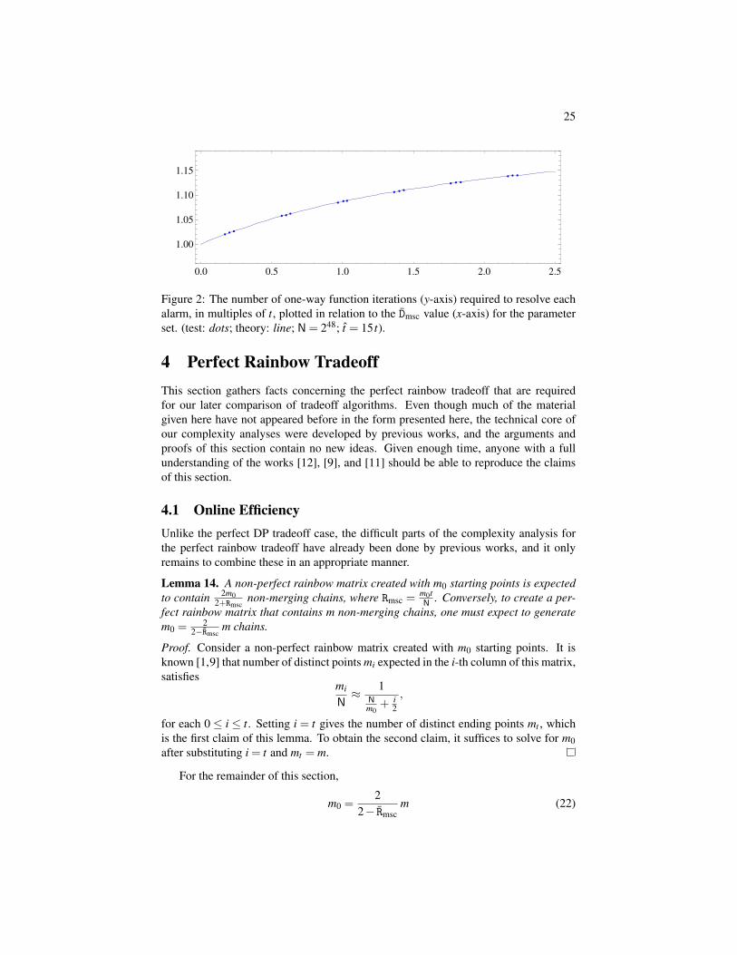
The results of our experiments, together with the predictions given by formula (18),are summarized in Table 2. We have also plotted the experiment data of Table 2 and thecurve given by formula (18) in Figure 2. The test value given in each row of the table isan average obtained after creating “#(tbl)”-many tables and generating, for each table,as many online chains as was required to obtain “#(alarm)/tbl”-many alarms. Eachvalue computed through formula (18) is very close to the average number of one-wayfunction iterations required per alarm that was obtained experimentally. Also, afterviewing Figure 2, one can be confident that formula (18) will be quite accurate, at leastfor all parameter choices satisfying 0 < Dmsc < 2.3.

24

Table 2: The number one-way function iterations required to resolve each alarm forvarious parameters. (N= 248; t = 15 t).

parameters test formula testformula

m0 m tDmsc

1t ×#(itr) 1

t ×Eq.(18)#(tbl) #(alarm) / tbl3000 2766 131072 0.16882 1.02002 1.01977 1.000251280 10000

231000 209976 16384 0.20025 1.02354 1.02314 1.00039128 3000017000 15230 65536 0.23239 1.02616 1.02650 0.99967640 1000048000 37354 65536 0.56998 1.05758 1.05713 1.00042128 1000012775 9843 131072 0.60077 1.05889 1.05956 0.99937640 5000

870000 661405 16384 0.63077 1.06202 1.06187 1.00014128 200001504000 1013856 16384 0.96689 1.08460 1.08483 0.99978128 2000099000 65884 65536 1.00531 1.08758 1.08715 1.00039128 100006400 4223 262144 1.03101 1.08824 1.08867 0.999611280 100009400 5588 262144 1.36426 1.10606 1.10642 0.999671280 10000

156000 91761 65536 1.40016 1.10806 1.10814 0.99993128 200002576000 1501280 16384 1.43173 1.10999 1.10962 1.00033128 20000217500 115580 65536 1.76361 1.12370 1.12377 0.99994128 200003587000 1887750 16384 1.80030 1.12553 1.12519 1.00030128 2000014400 7512 262144 1.83398 1.12610 1.12647 0.999671280 1000074000 35512 131072 2.16748 1.13818 1.13810 1.00007128 10000

4845000 2307050 16384 2.20017 1.13976 1.13915 1.00054128 20000310000 146425 65536 2.23427 1.14000 1.14022 0.99981128 20000

25

• ••

• • •

• • •

• • •

• • •• • •

0.0 0.5 1.0 1.5 2.0 2.5

1.00

1.05

1.10

1.15

Figure 2: The number of one-way function iterations (y-axis) required to resolve eachalarm, in multiples of t, plotted in relation to the Dmsc value (x-axis) for the parameterset. (test: dots; theory: line; N= 248; t = 15 t).

4 Perfect Rainbow TradeoffThis section gathers facts concerning the perfect rainbow tradeoff that are requiredfor our later comparison of tradeoff algorithms. Even though much of the materialgiven here have not appeared before in the form presented here, the technical core ofour complexity analyses were developed by previous works, and the arguments andproofs of this section contain no new ideas. Given enough time, anyone with a fullunderstanding of the works [12], [9], and [11] should be able to reproduce the claimsof this section.

4.1 Online EfficiencyUnlike the perfect DP tradeoff case, the difficult parts of the complexity analysis forthe perfect rainbow tradeoff have already been done by previous works, and it onlyremains to combine these in an appropriate manner.

Lemma 14. A non-perfect rainbow matrix created with m0 starting points is expectedto contain 2m0

2+Rmscnon-merging chains, where Rmsc =

m0tN . Conversely, to create a per-

fect rainbow matrix that contains m non-merging chains, one must expect to generatem0 =

22−Rmsc

m chains.

Proof. Consider a non-perfect rainbow matrix created with m0 starting points. It isknown [1,9] that number of distinct points mi expected in the i-th column of this matrix,satisfies

mi

N≈ 1

Nm0

+ i2

,

for each 0 ≤ i ≤ t. Setting i = t gives the number of distinct ending points mt , whichis the first claim of this lemma. To obtain the second claim, it suffices to solve for m0after substituting i = t and mt = m.

For the remainder of this section,

m0 =2

2− Rmscm (22)

26

will always denote the number of starting points that are required to create a perfectrainbow table containing m non-merging chains.

An interesting situation is when m0 = N, which is commonly referred to as themaximal perfect rainbow tradeoff [1]. Since a larger number of starting points m0brings about a larger number of non-merging ending point m, this is also the case forwhich Rmsc =

mtN is at its largest. With an easy manipulation of (22) after substitution

of m0 = N, one finds that there is an upper bound

Rmsc ≤2t

t +2< 2 (23)

on the possible range of Rmsc.The pre-computation phase of a perfect rainbow tradeoff requires m0t` iterations of

the one-way function. As in the DP case, we define the pre-computation coefficient forthe perfect rainbow tradeoff to be Rpc =

m0t`N , so that the number of one-way function

iterations required for pre-computation becomes RpcN. The following statement is adirect consequence of Lemma 14.

Proposition 15. The pre-computation coefficient of the perfect rainbow tradeoff is

Rpc =2

2− Rmsc

mt`N

=2 Rmsc

2− Rmsc`.

The success probability of a perfect rainbow tradeoff may easily be stated [1] as

Rps = 1−(

1− mN

)t`= 1− exp

(− mt`

N

)= 1− exp

(− Rmsc`

), (24)

and this shows that the choice of ` determines the matrix stopping constant

Rmsc =−ln(1− Rps)

`(25)

one must adhere to, when selecting parameters that achieve a prescribed probability ofsuccess. However, one must keep in mind that (23) requires for the number of tables tosatisfy

` >−12

ln(1− Rps). (26)

That is, to achieve a given success probability Rps, the number of tables one must useis lower bound by (26). No set of parameters that uses a smaller number of tables canachieve the desired success probability.

Using Proposition 15, we can restate the probability of success (24) as follows.

Proposition 16. The success probability of the perfect rainbow tradeoff is

Rps = 1− exp(− 2− Rmsc

2Rpc

).

Acquiring the online efficiency of the perfect rainbow tradeoff from existing worksis also straightforward.

27

Theorem 17. The time memory tradeoff curve for the perfect rainbow tradeoff isT M2 = RtcN

2, where the tradeoff coefficient is

Rtc =(Rmsc`−

Rmsc

2+ `−2+

32`

)−( R2

msc`

4+ Rmsc`

2− Rmsc`+ Rmsc + `−2+32`

)e−Rmsc`.

Proof. According to [9], the expected number of one-way function iterations requiredto generate the online chain is

`{

1− (1+ Rmsc`)e−Rmsc`}( t

Rmsc`

)2,

and that required to resolve alarms is4

{Rmsc

(`− 1

2

)−(

2− 32`

)}+{(

2− 32`

)+ Rmsc(`−1)− R2

msc`

4

}e−Rmsc`

( tRmsc`

)2.

These expected values take the possibility of premature exit from the online phase afterdiscovery of the correct answer into account. The sum of these two terms is the timecomplexity T . We can combine this with the storage complexity M = m` and thensimplify to arrive at the claim.

4.2 Storage OptimizationAs with the perfect DP tradeoff, storage of a single starting point for the perfect rainbowtradeoff requires logm0 bits, and (22) shows how this compares with logm. However,unlike the DP case, since Rmsc may take values that are very close to 2, there remainsthe possibility of logm0 being much larger than logm.

A hint for resolving this problem comes from the derivation process of (23), whichshows that Rmsc being close to 2 is associated with an unrealistically large amountof pre-computation. In any real-world situation, there will be a bound on the pre-computation cost one is willing to accept. So, let us combine Proposition 15 and (25),and consider a somewhat arbitrary bound of

Rpc =2

2− Rmsc

{− ln(1− Rps)

}≤ 20, (27)

on the pre-computation coefficient. Unless the requirement on the success rate is un-realistically small, this will place a reasonably small bound on the coefficient 2

2−Rmscof (22), so that logm will be similar to logm0. This shows that, for any practical sit-uation, it suffices to allocate slightly more than logm bits of storage to each startingpoint.

One side effect of (27) is that it implies the bound Rps ≤ 1− 1e20 on the suc-

cess probability one can consider. However, the appearance of a success probability

4The single ecR appearing in [9, p.312] should be corrected to ecR`.

28

bound is only natural, since a success probability that is arbitrarily close to 1 can-not be achieved without enormous amount of pre-computation. Furthermore, since99.999999% < 1− 1

e20 , the implied bound on the success probability is essentiallymeaningless for even a moderately large bound on the pre-computation cost.

The ending point truncation technique is the subject of our next discussion. In thecase of the perfect DP tradeoff, truncation was defined only for the DPs, but endingpoints may take any form with the rainbow tradeoff, so we now consider truncation ofany point from N . Consider a truncation method for which two random points of N ,truncated in the specified manner, will have probability 1

r of matching with each other.As before, we express such a situation as having 1

r probability of truncated match. Onespecific way to do this would be to truncate to logr most significant bits.

As in the DP case, truncation may cause two ending points of a perfect rainbowtable to become indistinguishable. Concerning this matter, Lemma 11 remains validfor the rainbow tradeoff.

Lemma 18. Assume the use of a truncation method with the truncated match proba-bility set to 1

r . If m distinct ending points of a perfect rainbow matrix are truncated,then we can expect to find r

{1−exp(−m

r )}

distinct truncated points. Conversely, whenr >m, one must expect to truncate r ln

( rr−m

)ending points in order to collect m distinct

truncated points.

The example values that were given below Lemma 11 remain valid for the perfectrainbow tradeoff. That is, truncation of 1.01596m ending points will give m distincttruncated points, when r = 25m. Hence, the effects of ending point truncation on pre-computation cost and success probability can be suppressed to an ignorable degree bythe use of an 1

r such that logr = ε + logm for some small positive integer ε .Analogous to the DP case, if required, one can work with (22) to find the correct

m0 value one must use in order to collect the slightly larger number of non-mergingpre-computation chains. Note that our previous discussion of how Rmsc is sufficientlybounded away from 2, in practice, implies that the non-linearity hidden within Rmscwill not cause too much disturbance. In particular, our claim of each starting pointrequiring logm0 ≈ logm bits of storage remains valid even if one wants to account forthe small loss of pre-computation chains experienced through the truncation of endingpoints.

The effect of truncation on the online time is considered next.

Lemma 19. Assume the use of ending point truncation with the truncated match prob-ability set to 1

r . Further assume that r has been chosen to be large enough so that theoccurrences of indistinguishable ending points from truncations are sufficiently limitedto be ignored. Then, during the online phase of the perfect rainbow tradeoff, one canexpected to observe

(Rmsc`

2− Rmsc`+Rmsc

2− `+2− 3

2`

)+( R2

msc`

4− Rmsc`+ Rmsc + `−2+

32`

)e−Rmsc`

mr

( tRmsc`

)2

extra one-way function invocations induced by truncation-related alarms.

29

Proof. Consider the non-perfect rainbow matrix created with m0 = 2m2−Rmsc

startingpoints and let mi (0 ≤ i ≤ t) denote the number of distinct points expected in the i-thcolumn of this matrix. The probability for the online chain created at the i-th iteration,i.e., the online chain of length i, starting from the correct inversion target pre-image,not to merge into the perfect rainbow matrix, but have an ending point that truncates toa truncated matrix ending point is

mr

i

∏j=0

(1−

mt− j

N

)≈ m

r

Nm0

+ t−i−12

Nm0

+ t2

Nm0

+ t−i−22

Nm0

+ t−12

≈ mr

( Nm0

+ t−i2

Nm0

+ t2

)2=

mr

(1− Rmsc

2it

)2.

Here, the first approximation relies on miN ≈

(Nm0

+ i2

)−1, which may be found in [1,9].The expected number of extra one-way function iterations induced by truncation-

related alarms is given by

`t

∑i=0

(t− i)mr

(1− Rmsc

2it

)2(1− m

N

)`(i−1),

for the (expected) processing of the ` rainbow tables. Here, the `(i−1)-th powered termgives the probability for the i-th iteration of the online phase algorithm to be executed.Unless t is very small, this can be approximated by

t2`mr

∫ 1

0(1−u)

(1− Rmsc

2u)2

exp(− Rmsc`u

)du.

Explicit computation of this definite integral results in our claim.

Recall that the total online time, without ending point truncation, was given duringthe proof of Theorem 17. It is straightforward to express the effects of ending pointtruncation on the total online time.

Proposition 20. Suppose that the online phase of a perfect rainbow tradeoff implemen-tation that stores each ending point in full requires T iterations of the one-way functionto complete. Consider the use of the ending point truncation with the truncated matchprobability set to 1

r , where logr = ε + logm. If ε is large enough for the effects oftruncation on pre-computation chain collision to be ignored, then the implementationwith the ending point truncation requires

−( 3

2` −2− Rmsc2 + `+ Rmsc`− Rmsc`

2)+( 3

2` −2+ Rmsc + `− Rmsc`+R2

msc`4

)e−Rmsc`( 3

2` −2− Rmsc2 + `+ Rmsc`

)−( 3

2` −2+ Rmsc + `− Rmsc`+R2

msc`4 + Rmsc`2

)e−Rmsc`

T2ε

additional iterations of the one-way function to complete.

For the typical parameters of Rmsc = 1 and ` = 1, the claim is that 0.774568 T2ε

additional one-way function iterations are expected due to truncation-related alarms.At ε = 5, this is 0.0242052T , which implies a 2.42% increase in online time due toending point truncation.

Let us summarize the issue of storage optimization for the perfect rainbow tradeoff.Each starting point can be stored in slightly more than logm bits. Each ending point

30

can be truncated to slightly more than logm bits with little effect on the success prob-ability, pre-computation cost, and online time. The index file technique can be used toremove almost logm further bits per ending point without any loss of information. Inall, storage of each starting point and ending point pair requires a little more than logmbits. Even though this is identical to the conclusion obtained in [11] for the non-perfectrainbow tradeoff, the analysis had to be repeated here for the perfect rainbow tradeoff.

5 Tradeoff Algorithm Performance ComparisonsFormulas for the success rates, online efficiencies, and pre-computation costs of theperfect DP and perfect rainbow tradeoffs were obtained in the previous two sections.This information is used in this section to understand the performances of the twoalgorithms.

5.1 Method of ComparisonLet us briefly summarize the arguments of [11, Section 8.1] that suggest how to com-pare different tradeoff algorithms.

• Different algorithms should be compared at parameters that achieve the sameprobability of success.

• The tradeoff coefficient is a measure of the online efficiency of an algorithm.However, one must keep in mind that the unit of storage used while computingthe tradeoff curve was the number of entries written to the pre-computation ta-ble, rather than the physical amount of required storage space. Hence, one mustaccount for the number of bits required to store each entry, which may be dif-ferent among algorithms, when comparing the tradeoff coefficients of differentalgorithms against each other. In the case of the classical Hellman, non-perfectDP, and non-perfect rainbow tradeoffs under typical environments, it is reason-able to compare the adjusted tradeoff coefficients Htc, 1

4Dtc, and Rtc against eachother.

• For any one tradeoff algorithm, a parameter set that achieves better online ef-ficiency usually calls for a larger amount of pre-computation. The appropriatebalance between these two factors will be different for every user and situation,and the comparison of algorithm performances can only be a subjective matter inthis respect. What can be done objectively is to present the pre-computation costversus online efficiency relation for each algorithm as graphs. The final decisionas to which algorithm is most suitable can be made by the user, for the specificsituation in hand, based on this information.

We will follow this approach in comparing the perfect DP and perfect rainbowtradeoff algorithms against each other. Recall that the classical Hellman, non-perfectDP, and non-perfect rainbow tradeoffs were compared in [11], and that the rainbowtradeoff could be seen as outperforming the other two in typical situations. All our

31

graphs given below include the information for the non-perfect rainbow tradeoff, sothat the two perfect table tradeoff algorithms analyzed in this work may also be roughlycompared against the three non-perfect table tradeoff algorithms.

5.2 ComparisonsSince we are going to compare the tradeoff algorithms at a common fixed probabilityof success, the parameters Dps and Rps will now be treated as fixed constants. Thediscussions of Section 3.2 and Section 4.2 show that perfect versions of the DP andrainbow tradeoffs require approximately the same number of bits per table entry as theirnon-perfect counterparts running under comparable resources. One can conclude that afair comparison of online efficiencies would compare the adjusted tradeoff coefficients14 Dtc and Rtc against each other, and that these two adjusted tradeoff coefficients mayalso be directly compared against the non-perfect rainbow tradeoff coefficient Rtc.

Let us explain how one may plot the pre-computation coefficient versus tradeoffcoefficient curves for the two perfect tradeoff algorithms. One can derive

Dpc =2+ Dmsc

2 Dcr

{− ln(1− Dps)

}(28)

from Proposition 4, and since Proposition 8 expresses Dcr as a function of Dmsc, thepre-computation coefficient can be seen as a function of the single parameter Dmsc, aslong as Dps is treated as a constant. Similarly, Theorem 10 and Proposition 8 expressthe tradeoff coefficient Dtc as a function of the single parameter Dmsc. Thus the relationbetween Dpc and Dtc may be drawn as a curve parameterized by Dmsc.

It is important to understand that, even when the success rate Dps and curve param-eter Dmsc are fixed to specific values, there still remains a single degree of freedom inthe tradeoff algorithm parameters m, t, and `, with which one can realize the tradeoffbetween the online time T and the storage requirement M. That is, the ability of the DPalgorithm to provide tradeoffs between online time and storage requirement is unim-paired by restrictions on the success rate and the matrix stopping constant, and the Dtcvalue appearing with each (Dpc, Dtc)-pair represents an online efficiency with a fullyoperational time memory tradeoff opportunity.

To be more concrete, suppose one is given specific Dps and Dmsc values, togetherwith any T and M that satisfy the tradeoff curve of Theorem 10, where the tradeoffcoefficient Dtc is computed from the given Dps and Dmsc values. Then it is easy to checkthat the sequentially defined parameter set

t ={ DmscDcr

Dps

(1+

1+0.577Dmsc

1+0.451Dmsc

Dmsc

1+ Dmsc

)−1T} 1

2, (29)

m =DmscN

t2 , (30)

`=N

mtDcr

{− ln(1− Dps)

}(31)

satisfies the four requests or restrictions on Dps, Dmsc, T , and M. The equivalenceof (31) and (14) implies that the success rate Dps will be achieved with these parameters,

32

•

•

•

•

•

•

•

é

é

é

é

90%

0 2 4 6 8 10

0

1

2

3

4

5

6

•

•

•

•

•

•

•

•

•

•

éé

é

é

é

95%

0 2 4 6 8 10 12 14

0

2

4

6

8

••

••••••••••••••••

éééééééééé

99%

0 5 10 15 20 25 30

0

5

10

15

20

••

••

•••••••••••••••••••••••••••

ééééééééééééééééééé

99.9%

0 10 20 30 40 50 60

0

5

10

15

20

25

30

35

Figure 3: The tradeoff coefficients 14 Dtc (line), Rtc (dots), and Rtc (circles), with adjust-

ments suitable for direct comparison, in relation to their respective pre-computationcosts, at various success rates (x-axis: Dpc, Rpc, and Rpc; y-axis: 1

4 Dtc, Rtc, and Rtc).

while (30) ensures that the given Dmsc value is adhered to. Furthermore, since (29) andthe first equation in the proof of Theorem 10 are equivalent, the online phase is expectedto terminate in the requested time T . Finally, since both the storage requirement underthe above parameter set and the requested M value satisfy the same tradeoff curve,i.e., with common values of the online time and tradeoff coefficient, adherence to M isguaranteed.

Let us now explain how the performance curve for the the perfect rainbow trade-off may be plotted. One can combine (25) and Proposition 15 to express the pre-computation coefficient

Rpc =2

2− Rmsc

{− ln(1− Rps)

}=−

2` ln(1− Rps)

2`+ ln(1− Rps)(32)

as a function of the single variable `. Similarly, the substitution of (25) into the formulaof Theorem 17 results in an expression for Rtc that is given in terms of the single vari-able `. Thus, the relation between Rpc and Rtc may be drawn as a curve parameterizedby `. As with the DP tradeoff, possibility of tradeoffs between online time and storagerequirement remains unaffected by the restrictions on Rps and `.

The curves for the two perfect tradeoffs and the non-perfect rainbow tradeoff aregiven in Figure 3 for some specific success rates. Within each box, being lower is tohave better online efficiency and being closer to the left edge is to require less pre-computation. Hence, one may roughly interpret being situated closer to the lower leftcorner as displaying better performance.

33

••

••

••

••

••

••

éééé

éé

éé

ééé

99%

5.0 5.2 5.4 5.6 5.8 6.00

5

10

15

20

Figure 4: Tradeoff coefficient for perfect (dots) and non-perfect (circles) rainbow trade-offs in relation to their pre-computation costs at 99% success rate (x-axis: Rpc and Rpc;y-axis: Rtc and Rtc).

In each box, the filled dots represent the choice of (Rpc, Rtc)-pairs made availableby the perfect rainbow tradeoff, and the empty circles represent data for the non-perfectrainbow tradeoff. Each dot for the perfect rainbow tradeoff corresponds to an integer `value, with the rightmost dot corresponding to `= d− 1

2 ln(1− Rps)e, as determined bythe bound (26). Since the table count ` must be an integer, the available choices appearas a discrete set of points. Similar statements may be made for the circles that representdata for the non-perfect rainbow tradeoff. The single continuous curve in each boxrepresents data for the perfect DP tradeoff. Unless N is small, it is reasonable to treatthe parameter Dmsc =

mt2

N that was used to draw these graphs as a continuous variable,even though it originates from integers. One can numerically verify that the tradeoffcoefficient Dtc attains its minimum at Dmsc = 1.97255, regardless of the Dps value. Thelowest point, or the right end, of the curve in each box corresponds to Dmsc = 1.97255and the curve is drawn only for the parameter in the range Dmsc≤ 1.97255. Curve pointscorresponding to larger Dmsc values would be associated with worse online efficienciesat higher pre-computation costs, which would not be used.

It is quite clear from Figure 3 that the perfect DP tradeoff is less desirable thanthe perfect rainbow tradeoff, regardless of how one wants to balance online efficiencyagainst pre-computation cost. When these normal to high success rates are required,the perfect DP tradeoff is no match for the perfect rainbow tradeoff. It also seems fair toclaim that the perfect rainbow tradeoff is at an advantage over the non-perfect rainbowtradeoff, since it can approximately provide every option made available by the non-perfect rainbow, while providing many more options that cannot be approximated bythe non-perfect rainbow tradeoff. Furthermore, the perfect rainbow tradeoff presentsthe possibility of obtaining much better online efficiencies, although these must bepaid for with higher pre-computation costs. At the 90% success rate, and possiblyalso at the 95% success rate, the perfect DP tradeoff is likely to be more useful thanthe non-perfect rainbow tradeoff, unless one is extremely restrained in the amount ofpre-computation possible.

The success rates covered by Figure 3 are those that would be of practical interest.We acknowledge that for success rate requirements that are much lower, such as 25% or50%, the situation is somewhat different. One can easily verify through curves similarto those of Figure 3 that the use of the perfect DP tradeoff can be advisable at these lessinteresting low sucess rates.

The comments given so far should generally be acceptible, but when lowering the

34

pre-computation cost is immensely important, there remains a small possibility thatthe non-perfect rainbow tradeoff could be preferred over the perfect rainbow tradeoff.This is illustrated by Figure 4, which is an enlarged view of a narrow vertical stripfrom the 99% box of Figure 3. We have intentionally stretched the vertical strip inthe horizontal direction and have reduced the height, so that even a small differencein the pre-computation coefficient is felt as being significant. Even though some sac-rifice in the online efficiency is inevitable, the options provided by the non-perfectrainbow tradeoff now seem much more reasonable than previously felt when viewedfrom within Figure 3.

To summarize, when the online efficiency and pre-computation cost are both takeninto account, the perfect rainbow tradeoff is very likely to be advantageous over perfectDP, non-perfect rainbow, non-perfect DP, and classical Hellman tradeoffs, in typicalsituations. However, there may be special circumstances under which the preferencescould be different. For example, importance of lowering the pre-computation cost mayshift the preference towards the non-perfect rainbow tradeoff, and the need for fine-tuned parameter choices may make the perfect DP tradeoff, or even the non-perfect DPand classical Hellman tradeoffs, favorable at low success rate requirements.

Before ending this section, let us briefly add two remarks concerning the Dmsc =1.97255 value that minimizes the tradeoff coefficient Dtc. Even though our derivationof the formula for Dtc relied on the approximation (18), since the range in which (18) isaccurate contains the minimizing Dmsc value, one can be confident that Dmsc = 1.97255indeed provides a (local) minimum for Dtc. In the opposite direction, as was alreadydiscussed, since Dmsc values greater than 1.97255 will not be used, it suffices to restrictour attention to parameters in the 0 < Dmsc ≤ 1.97255 range.

6 ConclusionIn this work, we analyzed the execution complexity of the perfect DP tradeoff and com-puted its tradeoff coefficient. We also combined the existing results on the executioncomplexity of the perfect rainbow tradeoff to present its online efficiency. Using thisinformation, the performances of the perfect DP tradeoff and perfect rainbow tradeoffwere compared against each other. We also added the non-perfect rainbow tradeoff,which was shown to outperform the classical Hellman and non-perfect DP tradeoffs ina previous work [11], to our comparison. Our conclusion, in overly simplified terms,is that the perfect rainbow tradeoff is advantageous over the other four tradeoff algo-rithms.

On the surface, our conclusion may seem to be a repetition of the claim given by thearticle [12] that first introduced the rainbow tradeoff, but the two claims differ funda-mentally in their contents. The previous work [12] measured the storage size in termsof the number of table entries, but the physical storage size was considered in our com-parisons. Our comparison was based on the expected execution complexities, ratherthan the worst case complexities, which were used by [12]. Finally, our comparisonconsidered both the online efficiency and the cost of pre-computation, whereas onlythe optimal online behavior was considered by [12]. In other words, different conceptsof one algorithm being better than another algorithm were employed by [12] and this

35

work in comparing tradeoff algorithms.In addition to the conceptual differences which make our comparisons more mean-

ingful in practice than the previous claims of [12], there was also a difference in the ac-curacy of the two comparisons. The claim of [12] relied on parameter sets for differentalgorithms that were heuristically shown to bring about roughly corresponding successrates, but the parameter sets for different algorithms were conditioned to achieve ex-actly the same success rate in our comparison. In addition, our comparison, unlike thatof [12], fully accounted for the complexity of resolving false alarms, which constitutesa significant portion of the online time.

Despite our simplified conclusion of the perfect rainbow tradeoff outperformingthe other four algorithms, we do not rule out the possibility of encountering situa-tions where the conclusions could be different. One example would be when loweringthe pre-computation cost is immensely important. There may also be issues we haveignored, such as the possibility of loading a pre-computation table into fast memoryor table lookup characteristics, which could make the two DP tradeoffs, with smallerindividual tables, preferable over the two rainbow tradeoffs. Furthermore, recent im-plementation platforms such as GPUs, where the scheduling of the online computationneeds to be totally different from most computation platforms and accesses to largestorage are inconvenient, could call for a new analysis of the execution complexities.

It remains to verify whether any of the recent tradeoff algorithm variants that claimsuperiority over existing algorithms are truly advantageous over the perfect rainbowtradeoff.

A Chain Length Bounds and Parallelization of the DPTradeoff

Let us briefly comment on the two techniques for the DP tradeoff that were not con-sidered during our complexity analyses. Specifically, these were the upper and lowerbounds on the chain lengths and the parallel processing of tables during the onlinephase.

The use of chain length bounds will increase the number of pre-computation chainsthat are discarded, so that the amount of pre-computation must be increased in order tomaintain the success rate. The effect of chain length bounds on the online efficiencyis unclear, but making the pre-computation chain lengths shorter has the tendency toreduce chain merges and false alarms, so this could have a positive effect. However,a quick review of Figure 3 shows that no small enhancement in the online efficiencyis likely to make the perfect DP tradeoff more preferable over the perfect rainbowtradeoff, even if no penalty on the pre-computation cost was involved. Hence, thereseems to be little reason to consider the perfect DP tradeoff variant that utilizes chainlength bounds, except possibly at low success rates.

The work [8, 15] suggests that all the pre-computation tables be processed in par-allel, rather than sequentially, during the online phase. Parallel processing causes theshorter online chains to be treated before the longer ones, and since the online phaseis likely to terminate with the correct answer before any of the pre-computation tables

36

are fully processed, this leads to a larger portion of the online computation being spenton processing the shorter chains. Since shorter chains are less likely to induce falsealarms, this has a positive effect of reducing the cost of dealing with alarms. How-ever, the recent analysis on the non-perfect parallel DP tradeoff [10] indicates that onecannot hope to see any drastic improvement of the perfect DP tradeoff performancethrough parallelization. For now, there seems to be no reason to expect the parallel per-fect DP tradeoff to perform better than the perfect rainbow tradeoff, especially underthe high success rate requirements which are of interest.

B Detailed Proof of Lemma 5The very short proof of Lemma 5 given in the main body of this paper will seem suffi-cient to most cryptographers. However, there are subtle issues involving random func-tions that were ignored in the proof. This section is an attempt at resolving these issues.We strongly urge any interested reader to review [11, Appendix B] before reading thissection.

Recall that we are using Dk(F) to denote the set of elements of N that are k-manyF-iterations away from their closest DPs, and suppose that D0, D1, . . . , Dk are anycollection of mutually disjoint subsets of N , with D0 denoting the set of all DPs. Letus consider any function F : N →N and discuss when the series of conditions

C1: Di = Di(F), for i = 1, . . . ,k

would be satisfied by the function. Note that the omitted condition D0 = D0(F) isalways satisfied.

The series of conditions C1 is satisfied by the function F if and only if the followingthree items are all satisfied:

C2: Di = Di(F), for i = 1, . . . ,k−1.

C3: F(Dk)⊂ Dk−1.

C4: F(N \Dk)∩Dk−1 = /0.

Repeating this argument, we see that the satisfaction of Condition-C1 by an F is equiv-alent to the satisfaction of the following two series of conditions.

C5: F(Dk)⊂ Dk−1, . . . , F(D2)⊂ D1, and F(D1)⊂ D0.

C6: F(N \Dk)∩Dk−1 = /0, . . . , F(N \D2)∩D1 = /0, and F(N \D1)∩D0 = /0.

Suppose that we were trying to construct a function that satisfies these conditions.Then the condition F(Dk)⊂ Dk−1 would certainly places a restriction on how we maydefine F on Dk. However, since the set Dk does not overlap with any of the othersets D0, . . . ,Dk−1, none of the other sub-conditions of C5 places any restriction on thedefinition of F on Dk. Next, the sub-condition F(N \Dk)∩Dk−1 = /0 of C6 is certainlyirrelevant to the definition of F on Dk. The other sub-conditions of C6 are not quite soirrelevant, but since Dk−1 does not overlap with any of the sets D0, . . . ,Dk−2, as long

37

as the condition F(Dk) ⊂ Dk−1 is adhered to, they are automatically satisfied and donot places any additional restriction of how we may define F on Dk. More generally,for each i = 1, . . . ,k, the condition F(Di) ⊂ Di−1 is the only restriction placed on thedefinition of F on Di by C5 and C6. In other words, asking for C1 to be satisfied bya function F places no restriction on the definition of F on Di other than that F(Di)⊂Di−1 be satisfied.

The discussion given so far can be reinterpreted as follows. Let D0,D1, . . . ,Dkbe any collection of mutually disjoint subsets of N , with D0 denoting the set of allDPs. By choosing a function F : N →N satisfying Condition-C1, one determinesfunctions Fi : Di → Di−1 for each i = 1, . . . ,k. Let us fix any i. If the choice of F ismade uniformly at random from the set of all function satisfying Condition-C1, thedistribution of the corresponding Fi : Di → Di−1, defined on the set of all functionshaving domain Di and codomain Di−1, also becomes the uniform distribution.

We are now ready to prove the lemma. Choose any explicit family of disjointsets D0, . . . , Dk such that D0 is the set of all DPs. For a random function satisfyingCondition-C1, since each Fi : Di→ Di−1 is a random function, we can expect to see

|F(D′)||Di−1|

= 1− exp(− |D′||Di−1|

)(33)

for every set D′ ⊂ Di and i = 1, . . . ,k. So far, we have fixed D0, . . . , Dk first and haveclaimed information on iterated image sizes only for functions F satisfying Condition-C1, which is associated with the sets D0, . . . , Dk. However, observe that this iterativeequation depends only on the set sizes |D′|, |D0|, . . . , |Dk| and not on the specific setsD′,D0, . . . ,Dk. Also recall that (15) is expected of a random function. Interpreting thisas (15) holding accurately for the vast majority of functions F , the truth of Lemma 5follows. A review of [11, Appendix B] is required to fully understand this final state-ment.

C Comments on a Previous Analysis of the perfect DPTradeoff

Since there is a large overlap between what the previous work [16] and the currentwork claim to have obtained, let us compare some of the results from the two works.

The paper [16] provides a method for computing the number of distinct ending DPsexpected from a given number of starting points. This value, which is the number ofchains remaining after removal of merging chains, was referred to as α in Section 2.2.In Table 3, we have copied some of the related data appearing in [16, Table 2] andhave appended our corresponding theoretical values, computed with Lemma 2. Theparameters associated with this table are N = 256 and t = 218, and all figures in thetable are given as log2 values. Recall that Lemma 2 is valid for the case when no chainlength bounds are set. The data from [16] are for when there is no lower bound on thechain length and the chain length upper bound is set to 230, which is sufficiently largefor the t = 218 being used.

38

Table 3: Number of DP chains before and after removal of chain merges (N = 256,t = 218). All values are given in log2 scale.

# of startingpoints

# of ending pointstest of [16] theory of [16] Lemma 2

20 19.5497 19.4712 19.550021 20.3048 20.1357 20.305822 20.9990 20.6866 21.000023 21.6425 21.1357 21.6430

One can verify, in every row of the table, that our theory provides estimates that arecloser to the test results of [16] than their own theory. Some might dismiss the differ-ences between the two theoretical values as being too small to be of any significance,but one must consider the fact that these are log2 values. For example, referencingthe last row of the table, we can see that the (in)accuracy of Lemma 2 in predictingthe test value is by a factor of 221.6425

221.6430 ≈ 0.999653, but that the theoretical prediction

of [16] is further away at a factor of 221.6425

221.1357 ≈ 1.42. The error factor of 1.42 in the es-timated number of ending points is directly reflected in the pre-computation table sizeestimate and presents itself as a 1.422 ≈ 2.02 error factor in the estimate for the trade-off coefficient. Hence, for the purpose of comparing the online efficiencies of tradeoffalgorithms, which usually differ only by factors of such small magnitude, the theoryof [16] was not accurate enough.

Recall from Section 2.2 that the expression for α given in [16] involved the averagechain length β and that their derivation of β involved an ad hoc procedure. So, let usconsider the possibility that this ad hoc procedure was the cause of the inaccuracy wehave witnessed in Table 3 and that their arguments were correct up to that point. Forthis purpose, we focus on one major intermediate result of [16] which they refered toas the storage function s( j).

The exact definition of s( j) is slightly complicated and will not be explained herein full, but when no bounds are placed on the chain lengths, function s( j) is supposeto give the expected number of distinct nodes in a perfect DP matrix that was createdwith j starting points. The formula they gave was

s( j) = 2k{

1−( 2k

−β j+β 2 j+K

) 1β−1}

with K = 2k(

1− s(0)2k

)1−β

, (34)

where the β they used was the average chain length before the removal of chain mergesand 2k was the size of the search space. The presence of s(0) may seem strange, butthis is because we have not explained the meaning of s( j) in full, and we may simplytake s(0) = 0 for this discussion. In the absence of chain length bounds, we may takeβ = t and approximate their formula into

s( j) = N{

1−( N

t2 j+N

) 1t}, (35)

written in the notation of this paper. Hence, according to the theory of [16], if one

39

lnH1+DmscL

2 lnH1+ 1 +2 Dmsc

2L

0 1 2 3 4

0.0

0.5

1.0

1.5

Figure 5: The value tN |DM|= DmscDcr as predicted by [16] (solid) and the current work

(dashed). (x-axis: Dmsc; y-axis: tN |DM|)

creates a perfect DP matrix using m0 starting points, there will be

|DM|= s(m0) = N{

1−( 1

1+Dmsc

) 1t}

(36)

distinct points in the matrix, where Dmsc =m0t2

N . To allow for direct comparison withour result, we rewrite this in the form

tN|DM|= t

{1−( 1

1+Dmsc

) 1t}≈ ln(1+Dmsc). (37)

The approximation here is accurate for all sufficiently large t. For example, at Dmsc = 1the right-hand value is ln(1+Dmsc)= 1.09861, and even at the moderately sized t = 210,the formula in the middle involving t evaluates to 1.09802.

Our corresponding result is contained in Proposition 8. Using (12), we can claim

tN|DM|= DmscDcr = 2ln

(1+

Dmsc

2

)= 2ln

(1+√

1+2Dmsc

2

), (38)

which is clearly different from (37).The numeric values given by the two formulas (37) and (38) are compared in Fig-

ure 5. The two are visibly different, except when Dmsc is very small, in which casechain merges are rare and both theories reduce to something trivial. For example, evenat Dmsc = 1, the two theories give clearly different values of 0.69315 and 0.62381.Since the testing of Section 3.3 has shown our estimate of coverage rate to be muchmore accurate than the general order of these differences, the storage function s( j), asgiven by (35), must not be as accurate.

Let us explain the source of their inaccuracy. The core logic of [16] rests in theirEquation (22), which we approximate and state as

s( j+1) = s( j)+ t(

1− s( j)N

)t, (39)

for the case when there are no chain length bounds. This equation can be interpretedas follows. One expects to add t new points to the perfect matrix by considering one

40

more pre-computation chain, but this addition should only be done when the chain of tpoints do not merge with the points within the existing matrix. The t-th powered termon the right is the probability for none of the t additionally generated points to be inthe existing matrix of s( j) points. This high-level view of (39) may seem plausible.

The first source of inaccuracy hiding in (39) is the assumption that the new chainadded is always of length t. In reality, chains of varying lengths will be created andthese all have different probabilities of merging with the existing matrix. The simplifiedview of [16] could have been justified to a certain degree if the chain lengths weremostly close to t, but the actual distribution of chain lengths is not even centered atthe average value t. The authors of [16] seem to have been aware of this problem. Inlater parts of their paper, they divide the range of possible chain lengths into a smallnumber of segments and treat each length range separately, using different averagechain lengths within each segment.

The second source of inaccuracy is in the t-th powered term that was suppose togive the probability for the additional chain not to merge with the existing matrix. Sincewe are dealing with a DP chain of a predetermined length at this point, a more accu-rate expression would somehow involve the set sizes |Dk|, that appeared in the mainbody of this work, in the denominator, rather than N. Furthermore, the numerator s( j)should be replaced with values that are associated in some way with the non-perfectmatrix created up to that point. This is because the newly created chain is destined tomerge with the perfect matrix whenever it merges with a previously generated chain,regardless of whether the chain has been discarded due to merging.

We conclude that while the analyses of [16] are base on plausible arguments, theirresults are valuable only as first approximations and are not accurate enough for thepurpose of this paper, which is to compare the performances of different tradeoff algo-rithms.

D Optimal Rainbow Tradeoff ParametersIn this section we discuss the parameter set for the perfect rainbow tradeoff that theprevious analysis [1] suggested and claimed to be optimal. Let us explain the stepsthey take to fix the parameters, in the language of this work. The required successrate Rps and the total number of table entries M are treated as the externally suppliedparameters. First (26) is used to fix the number of tables ` = d− 1

2 ln(1− Rps)e. Thisforces the number of starting points per table to m = M

` and we know from (24) thatthe remaining parameter t must be fixed to

t =− N

m`ln(1− Rps) =−

N

Mln(1− Rps), (40)

if the requested success rate is to be achieved. In short, the number of tables is chosento be as small as possible, subject to the condition (26), and the rest of the parametersare set to what they must be in order to satisfy the externally given requirements.

It is not hard to show that the tradeoff coefficient Rtc of Theorem 17, when com-bined with (25), is an increasing function of ` in the range `≥ 1 and 0≤ Rps < 1. Thisimplies that the parameters suggested by [1] are optimal in the sense that it gives the

41

••

••••••

79%

0 1 2 3 4 5 6 7

0

1

2

3

••

••••••••••

82%

0 2 4 6 8 10 12

0

2

4

••••••••••••••••••••

84%

0 5 10 15 20

0

4

8

••••••••••••••••••••••••••••••••••

85%

0 10 20 30 40

0

5

10

15

•••••••••••••••••••••••••••••••••••••••••••••••••••••••••••••••••••••••••••••••••••••••••••••••••••••••

86%

0 20 40 60 80 100 120

0

20

40

••••••••••••••••••••••••••••••••••••••••••••••••••••••••••••••••••••••••••••••••••••••••••••••••••••••••••••••••••••••••••••••••••••••••••••••••••••••••••••••••••••••••••••••••••••••••••••••••••••••••••••••••••••••••••••••••••••••••••••••••••••••••••••••••••••••••••••••••••••••••••••••••••••••••••••••••••••••••••••••••••••••••••••••••••••••••••••••••••••••••••••••••••••••••••••••••••••••••••••••••••••••••••••••••••••••••••••••••••••••••••••••••••••••••••••••••••••••••••••••••••••••••••••••••••••••••••••••••••••••••••••••••••••••••••••••••••••••••••••••••••••••••••••••••••••••••••••••••••••••••••••••••••••••••••••••••••••••••••••••••••••••••••••••••••••••••••••••••••••••••••••••••••••••••••••••••••

86.4%

0 200 400 600 8000

100

200

300

Figure 6: Pre-computation cost versus tradeoff coefficient for the perfect rainbow trade-off at success rates slightly lower than 1− 1

e2 = 86.466% (x-axis: Rpc; y-axis: Rtc).

smallest possible tradeoff coefficient among those achieving the intended success rate.An easier approach would be to state that, the optimal parameter set of [1] correspondsto the rightmost filled dot in each box of Figure 3, which is clearly the lowest dot ineach box.

However, we want to emphasize that the rightmost dot of each box is just one ofthe many options that are available to the tradeoff algorithm implementer, and thatthis specific option is not likely to be favored over others when the pre-computationcost is taken into account, except possibly at low success rates. Furthermore, Figure 6demonstrates that there are success rates for which using parameters corresponding tothe rightmost dot is certainly impractical.

The parameter set that is most efficient in terms of online resource requirements isvery often not the most practical or reasonable parameter set option among those madeavailable by a tradeoff algorithm. The current work provides the information whichenables the tradeoff algorithm implementer to decide on the most sensible, rather thanthe most online-efficient, parameter to use.

References[1] G. Avoine, P. Junod, P. Oechslin, Characterization and improvement of time-

memory trade-off based on perfect tables. ACM Trans. Inform. Syst. Secur. 11(4),17:1–17:22 (2008). Preliminary version presented at INDOCRYPT 2005.

[2] E. Barkan, E. Biham, A. Shamir, Rigorous bounds on cryptanalytic time/memorytradeoffs, in Advances in Cryptology—CRYPTO 2006. LNCS 4117, (Springer,2006), pp. 1–21.

[3] A. Biryukov, A. Shamir, D. Wagner, Real time cryptanalysis of A5/1 on a PC, inFSE 2000. LNCS 1978, (Springer, 2001), pp. 1–18.

[4] J. Borst, Block Ciphers: Design, Analysis, and Side-Channel Analysis. Ph.D. The-sis, Katholieke Universiteit Leuven, September 2001.

[5] J. Borst, B. Preneel, J. Vandewalle, On the time-memory tradeoff between exhaus-tive key search and table precomputation, in Proceedings of the 19th Symposiumon Information Theory in the Benelux. (WIC, 1998), pp. 111–118.

42

[6] D. E. Denning, Cryptography and Data Security (Addison-Wesley, Reading,1982).

[7] M. E. Hellman, A cryptanalytic time-memory trade-off. IEEE Trans. on Infor.Theory 26, pp. 401–406 (1980).

[8] Y. Z. Hoch, Security analysis of generic iterated hash functions. Ph.D. Thesis,Weizmann Institute of Science, August 2009.

[9] J. Hong, The cost of false alarms in Hellman and rainbow tradeoffs. Des. CodesCryptogr. 57(3), pp. 293–327 (2010).

[10] J. Hong, G. W. Lee, D. Ma, Analysis of the parallel distinguished point tradeoff,in Progress in Cryptology—INDOCRYPT 2011. LNCS 7107, (Springer, 2011),pp. 161–180.

[11] J. Hong, S. Moon, A comparison of cryptanalytic tradeoff algorithms. J. Cryptol-ogy 26(4), pp. 559-637 (2013).

[12] P. Oechslin, Making a faster cryptanalytic time-memory trade-off, in Advances inCryptology—CRYPTO 2003. LNCS 2729, (Springer, 2003), pp. 617–630.

[13] J.-J. Quisquater, J. Stern, Time-Memory Tradeoff Revisited. Unpublished, De-cember 1998.

[14] N. Saran, Time Memory Trade Off Attack on Symmetric Ciphers. Ph.D. Thesis,Middle East Technical University, February 2009.

[15] A. Shamir, Random Graphs in Security and Privacy. Invited talk at ICITS 2009.

[16] F.-X. Standaert, G. Rouvroy, J.-J. Quisquater, J.-D. Legat, A time-memory trade-off using distinguished points: New analysis & FPGA results, in CryptographicHardware and Embedded Systems—CHES 2002. LNCS 2523, (Springer, 2003),pp. 593–609.

[17] M. J. Wiener, The full cost of cryptanalytic attacks. J. Cryptology 17(2), pp. 105–124 (2004).