A Comparison of Genetic Algorithmsusing Super Mario Bros.

An Major Qualifying Projectsubmitted to the Faculty of

WORCESTER POLYTECHNIC INSTITUTEin partial fulfillment of the requirements for the

degree of Bachelor of Science

byRoss FoleyKarl Kuhn

Date:30 April 2015

Report Submitted to:

Sonia ChernovaWorcester Polytechnic Institute

This report represents work of WPI undergraduate students submitted to the faculty asevidence of a degree requirement. WPI routinely publishes these reports on its web site

without editorial or peer review. For more information about the projects program at WPI,see http://www.wpi.edu/Academics/Projects.

Contents

1 Introduction 1

2 Background 22.1 Genetic Programming . . . . . . . . . . . . . . . . . . . . . . . . . . . . . . 22.2 Neural Networks . . . . . . . . . . . . . . . . . . . . . . . . . . . . . . . . . 3

2.2.1 Evaluation of Neurons . . . . . . . . . . . . . . . . . . . . . . . . . . 42.2.2 Learning . . . . . . . . . . . . . . . . . . . . . . . . . . . . . . . . . . 5

2.3 NeuroEvolution of Augmenting Topologies . . . . . . . . . . . . . . . . . . . 62.3.1 Basic Structure . . . . . . . . . . . . . . . . . . . . . . . . . . . . . . 62.3.2 Mutation . . . . . . . . . . . . . . . . . . . . . . . . . . . . . . . . . 62.3.3 Innovation Numbers . . . . . . . . . . . . . . . . . . . . . . . . . . . 72.3.4 Crossover . . . . . . . . . . . . . . . . . . . . . . . . . . . . . . . . . 72.3.5 Speciation . . . . . . . . . . . . . . . . . . . . . . . . . . . . . . . . . 8

2.4 Evolving Behavior Trees . . . . . . . . . . . . . . . . . . . . . . . . . . . . . 92.4.1 Crossover . . . . . . . . . . . . . . . . . . . . . . . . . . . . . . . . . 102.4.2 Mutation . . . . . . . . . . . . . . . . . . . . . . . . . . . . . . . . . 11

2.5 Super Mario Bros. . . . . . . . . . . . . . . . . . . . . . . . . . . . . . . . . 112.5.1 Mario AI Championship . . . . . . . . . . . . . . . . . . . . . . . . . 122.5.2 Competition Results . . . . . . . . . . . . . . . . . . . . . . . . . . . 122.5.3 Updated Competition . . . . . . . . . . . . . . . . . . . . . . . . . . 13

3 Methodology 143.1 Mario Level Parameters . . . . . . . . . . . . . . . . . . . . . . . . . . . . . 14

3.1.1 Training Levels . . . . . . . . . . . . . . . . . . . . . . . . . . . . . . 143.1.2 Test Levels . . . . . . . . . . . . . . . . . . . . . . . . . . . . . . . . 15

3.2 AI Controller Parameters . . . . . . . . . . . . . . . . . . . . . . . . . . . . . 153.2.1 Evolution Process . . . . . . . . . . . . . . . . . . . . . . . . . . . . . 153.2.2 Evaluating Fitness of Controllers . . . . . . . . . . . . . . . . . . . . 153.2.3 Feature Sets . . . . . . . . . . . . . . . . . . . . . . . . . . . . . . . . 15

3.3 NEAT . . . . . . . . . . . . . . . . . . . . . . . . . . . . . . . . . . . . . . . 163.4 EBT . . . . . . . . . . . . . . . . . . . . . . . . . . . . . . . . . . . . . . . . 173.5 Comparisons . . . . . . . . . . . . . . . . . . . . . . . . . . . . . . . . . . . . 18

4 Data and Analysis 204.1 Training Data . . . . . . . . . . . . . . . . . . . . . . . . . . . . . . . . . . . 20

4.1.1 NEAT . . . . . . . . . . . . . . . . . . . . . . . . . . . . . . . . . . . 214.1.2 EBT . . . . . . . . . . . . . . . . . . . . . . . . . . . . . . . . . . . . 224.1.3 Comparisons . . . . . . . . . . . . . . . . . . . . . . . . . . . . . . . 23

4.2 Rise Time . . . . . . . . . . . . . . . . . . . . . . . . . . . . . . . . . . . . . 24

1

4.3 Evolution Timing Data . . . . . . . . . . . . . . . . . . . . . . . . . . . . . . 254.4 Complexity . . . . . . . . . . . . . . . . . . . . . . . . . . . . . . . . . . . . 27

4.4.1 NEAT . . . . . . . . . . . . . . . . . . . . . . . . . . . . . . . . . . . 274.4.2 EBT . . . . . . . . . . . . . . . . . . . . . . . . . . . . . . . . . . . . 284.4.3 Comparisons . . . . . . . . . . . . . . . . . . . . . . . . . . . . . . . 30

4.5 Test Data . . . . . . . . . . . . . . . . . . . . . . . . . . . . . . . . . . . . . 304.5.1 Difficulty 0 Test Levels . . . . . . . . . . . . . . . . . . . . . . . . . . 314.5.2 Difficulty 1 Test Levels . . . . . . . . . . . . . . . . . . . . . . . . . . 33

4.6 Generalization . . . . . . . . . . . . . . . . . . . . . . . . . . . . . . . . . . . 34

5 Recommendations 365.1 When to use NEAT . . . . . . . . . . . . . . . . . . . . . . . . . . . . . . . . 365.2 When to use EBTs . . . . . . . . . . . . . . . . . . . . . . . . . . . . . . . . 36

6 Areas for Future Work 376.1 New Features . . . . . . . . . . . . . . . . . . . . . . . . . . . . . . . . . . . 376.2 Improved Training Levels . . . . . . . . . . . . . . . . . . . . . . . . . . . . . 376.3 Other AI Techniques . . . . . . . . . . . . . . . . . . . . . . . . . . . . . . . 38

7 Conclusion 39

2

List of Figures

2.1 Neural Network Structure . . . . . . . . . . . . . . . . . . . . . . . . . . . . . 42.2 NEAT Crossover Process [10] . . . . . . . . . . . . . . . . . . . . . . . . . . . 82.3 Example EBT . . . . . . . . . . . . . . . . . . . . . . . . . . . . . . . . . . . 102.4 2009 Mario AI Competition Results [6] . . . . . . . . . . . . . . . . . . . . . . 13

3.1 Mario Feature Set Grid for 7x7 Input [6] . . . . . . . . . . . . . . . . . . . . . . 16

4.1 NEAT Training Data Results . . . . . . . . . . . . . . . . . . . . . . . . . . . 214.2 EBT Training Data Results . . . . . . . . . . . . . . . . . . . . . . . . . . . . 224.3 Maximum Fitness Summary . . . . . . . . . . . . . . . . . . . . . . . . . . . . 234.4 Rise Time Summary . . . . . . . . . . . . . . . . . . . . . . . . . . . . . . . . 244.5 Evolution Timing Data . . . . . . . . . . . . . . . . . . . . . . . . . . . . . . . 254.6 NEAT Champion Complexity Over Time . . . . . . . . . . . . . . . . . . . . . 274.7 EBT Champion Complexity Over Time . . . . . . . . . . . . . . . . . . . . . . 284.8 3× 3 EBT from Generation 820 . . . . . . . . . . . . . . . . . . . . . . . . . . 294.9 3× 3 EBT from Generation 998 . . . . . . . . . . . . . . . . . . . . . . . . . . 294.10 NEAT vs. EBT Difficulty 0 Test Level Fitness . . . . . . . . . . . . . . . . . . . 314.11 NEAT vs. EBT Difficulty 0 Test Levels Completed . . . . . . . . . . . . . . . . 324.12 NEAT vs. EBT Difficulty 1 Test Level Fitness . . . . . . . . . . . . . . . . . . . 334.13 7× 7 NEAT Champion Stuck on Level Seed 32 . . . . . . . . . . . . . . . . . . 34

3

Abstract

This project was designed to compare and contrast Evolving Behavior Trees (EBTs) with

NeuroEvolution of Augmenting Topologies (NEAT), a Genetic Algorithm for the evolution

of Artificial Neural Networks. We used Super Mario Bros. as a benchmark to compare these

two techniques. The results showed that NEAT had a slightly higher maximum fitness while

performing poorly in all other comparisons. EBTs performed strongly in rise time, evolution

time, generalization, and complexity.

1 Introduction

Artificial intelligence (AI), while often portrayed negatively in movies, has impacted many

aspects of today’s society. Ranging from video game AI such as Left 4 Dead [2] to facial

recognition software [9], AI directly impacts how we view the world and what a computer is

capable of accomplishing. Just as society looks for smarter technology as the demand and

expectations rise, so too must the computers.

Ideally, society could have computers doing the majority of the routine tasks. However,

AI is not mature enough where computers are able to be so integrated into everyday life.

Looking at a smaller scale, we can do research into the learning ability and performance of

various AIs.

There are multiple variations of Genetic Algorithms (GA) that can produce an effective

AI, including Evolving Behavior Trees (EBT) and NeuroEvolution of Augmenting Topologies

(NEAT). The question is: how do they compare?

Our research determines the relative strengths and weaknesses of these forms of AI. By

doing so, we can gain a better understanding of when to apply one method over another.

We used the platform of Super Mario Bros. to compare our AIs into quantitative data. This

approach has been used before during competitions [11]. By comparing both methods on

the same platform, we were able to obtain clear information regarding the strengths and

weaknesses of both methods.

1

2 Background

2.1 Genetic Programming

The first paper published related to Genetic Programming (GP) was published in 1954

when Nils Aall Barricelli used evolutionary algorithms to try to simulate evolution [1]. Ten

years later, in 1964, Lawrence J. Fogel applied this theory of GP to finite state machines.

However, the first modern form of GP didn’t occur until 1985 when Nichael L. Cramer

applied these evolutionary algorithms to trees [4].

GAs are typically represented in binary strings; however, a variety of representations are

available [13]. The evolutionary process starts with random individuals, known as chromo-

somes. The collection of individuals are known as a population. Each generation consists of

a population of chromosomes. There are three operations to advance from one generation

to another.

Evaluation: Each individual is evaluated using a fitness function at the start of each gen-

eration. This function assigns a numeric fitness to each individual, making it possible

to compare individuals.

Selection: At the end of each iteration of the algorithm, the strongest individuals will both

advance and go through crossover to create the next generation.

Crossover: Crossover, also known as breeding, is the action of swapping portions of in-

formation between two individuals in the population. For example, for a tree-based

GA, the act of crossover would be taking a branch from one tree (one individual) and

swapping it with another tree’s branch. This action creates two different child trees

that are noticeably different from their parents. The goal of the crossover is to create

2

new individuals who are superior to their parents. However, crossover by itself is not

sufficient to create significant changes from generation to generation.

Mutation: To add more variation to each generation, individuals should occasionally be

mutated. This means randomly changing various bits of information of an individual.

In the tree example, an individual could be mutated by taking one of its branches and

replacing it with another random branch. After a mutation has occurred, it can then

crossover with other individuals, diffusing the new information into the population.

Genetic Algorithms will typically run continuously, converging slowly to the optimal so-

lution. However, by default, GAs do not terminate. In order to stop the program from

infinitely looping, the GA must have a termination case. There are multiple ways of accom-

plishing this, including minimum solution, number of generations, computation time, and a

plateau test. The minimum solution termination case makes the GA accept a solution if it

meets the bare minimum requirements to complete the problem. A GA can also stop after

a fixed number of generations. One could also let the GA run until a time or computation

limit is reached. Lastly, the plateau test stops the GA after the fitness of each generation

has stopped increasing.

There are many GP techniques available, such as extended compact genetic programming

or probabilistic incremental program evolution. These techniques modify and extend the

ideas of genetic programming to solve specific types of problems. However, the following

experiments will focus on exploring both an evolving behavior tree and a neural network

implementation of GAs.

2.2 Neural Networks

A neural network is an artificial intelligence technique inspired by how the brain works

[12]. It consists of a set of neurons with weighted connections between them. Neurons can

either be inputs, outputs, or hidden.

3

Input: Input neurons are given values based on input to the model being trained. In the

case of Super Mario Bros., this would be information such as Mario’s current power-up

state, the locations of enemies, and the locations of blocks.

Output: Output neurons represent the output of the model. In the case of Super Mario

Bros., this would be button presses. For example, if the output neuron representing

the run button had a value of 1, then the AI controller would press the run button.

Hidden: Hidden neurons are used to add more detail to the output of the neural network.

If the original neural network’s output was represented by the function f(x), then

adding a layer of hidden neurons would make the output g(f(x)), where g(x) is the

hidden neuron’s activation function. Essentially, they act as if you fed the output of

one neural network into the input neurons of another neural network. This allows for

more complex functions to be modeled by the neural network, such as discontinuous

functions.

Input 1

Input 2

Input 3

Input 4

Hidden 1

Hidden 2

Output 1

Output 2

Figure 2.1: Neural Network Structure

2.2.1 Evaluation of Neurons

The output of each neuron is determined by its inputs and its activation function [3].

The input value for a neuron (inj) is determined by the value of each input (xi) and its

4

weight (wi):

inj =∑i

wi · xi (2.1)

The output of a neuron is then computed using its activation function (g(x)):

outj = g(inj) (2.2)

There are many possibilities for the activation function. The most basic function would

be one that outputs 1 if inj >= 0 and 0 if inj < 0. A more complex example would be a

differentiable function, such as the sigmoid function:

g(inj) =1

1 + e−inj

p

p ∈ R (2.3)

2.2.2 Learning

There are many ways to train the weights of a neural network. One of the most common

methods is called backpropogation [12]. Backpropogation is a form of supervised learning

where the neural network is trained based on a set of training data. The training data

consists of the values for the input neurons and the expected values of the output neurons.

At each step, the neural network is fed the training inputs and the actual output values are

recorded. Then, the difference between the expected and actual output is used to update

the weights of the neural network. This can be repeated as many times a necessary until the

neural network is within the desired level of accuracy.

Supervised learning works well when it is feasible to create a large enough set of training

data to train the neural network with. However, this can be difficult for a game like Super

Mario Bros. where human error is almost impossible to avoid. Therefore, a more effective

technique would utilize reinforcement learning to avoid introducing human error into the AI

controller.

5

2.3 NeuroEvolution of Augmenting Topologies

One form of reinforcement learning that has proven extremely effective is NeuroEvolution

of Augmenting Topologies (NEAT) [10]. NEAT combines genetic programming with neural

networks to create a technique that is not only capable of finding the correct weights, but

also the correct topology of a neural network.

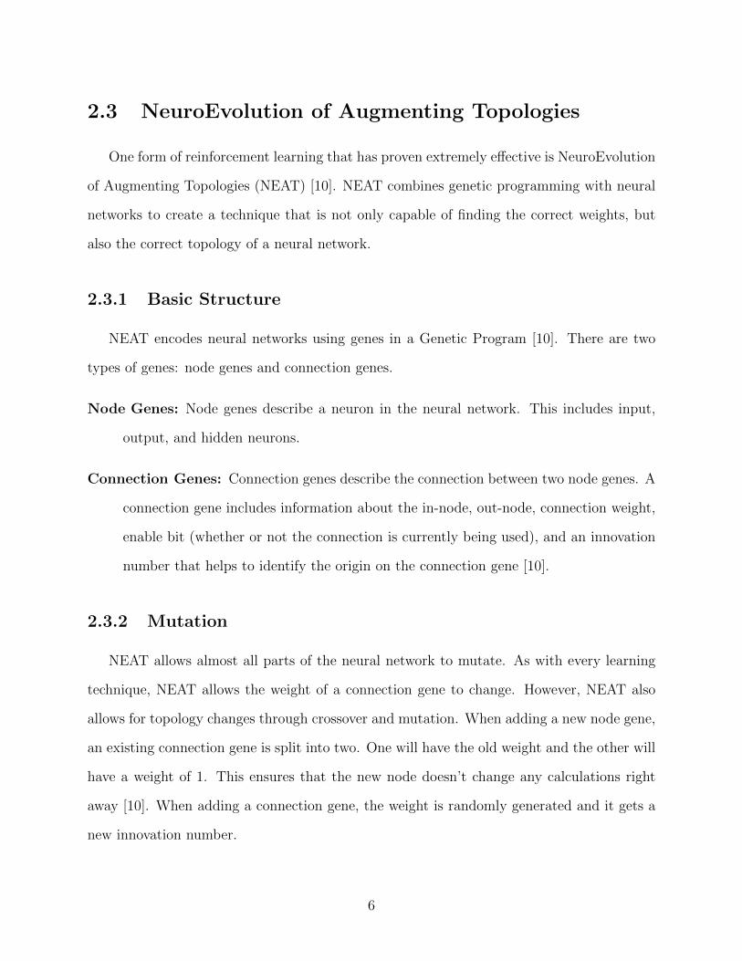
2.3.1 Basic Structure

NEAT encodes neural networks using genes in a Genetic Program [10]. There are two

types of genes: node genes and connection genes.

Node Genes: Node genes describe a neuron in the neural network. This includes input,

output, and hidden neurons.

Connection Genes: Connection genes describe the connection between two node genes. A

connection gene includes information about the in-node, out-node, connection weight,

enable bit (whether or not the connection is currently being used), and an innovation

number that helps to identify the origin on the connection gene [10].

2.3.2 Mutation

NEAT allows almost all parts of the neural network to mutate. As with every learning

technique, NEAT allows the weight of a connection gene to change. However, NEAT also

allows for topology changes through crossover and mutation. When adding a new node gene,

an existing connection gene is split into two. One will have the old weight and the other will

have a weight of 1. This ensures that the new node doesn’t change any calculations right

away [10]. When adding a connection gene, the weight is randomly generated and it gets a

new innovation number.

6

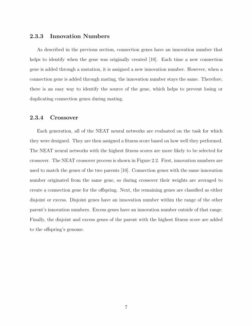
2.3.3 Innovation Numbers

As described in the previous section, connection genes have an innovation number that

helps to identify when the gene was originally created [10]. Each time a new connection

gene is added through a mutation, it is assigned a new innovation number. However, when a

connection gene is added through mating, the innovation number stays the same. Therefore,

there is an easy way to identify the source of the gene, which helps to prevent losing or

duplicating connection genes during mating.

2.3.4 Crossover

Each generation, all of the NEAT neural networks are evaluated on the task for which

they were designed. They are then assigned a fitness score based on how well they performed.

The NEAT neural networks with the highest fitness scores are more likely to be selected for

crossover. The NEAT crossover process is shown in Figure 2.2. First, innovation numbers are

used to match the genes of the two parents [10]. Connection genes with the same innovation

number originated from the same gene, so during crossover their weights are averaged to

create a connection gene for the offspring. Next, the remaining genes are classified as either

disjoint or excess. Disjoint genes have an innovation number within the range of the other

parent’s innovation numbers. Excess genes have an innovation number outside of that range.

Finally, the disjoint and excess genes of the parent with the highest fitness score are added

to the offspring’s genome.

7

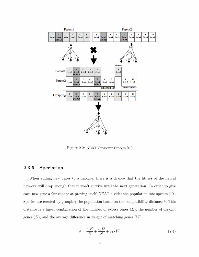
Figure 2.2: NEAT Crossover Process [10]

2.3.5 Speciation

When adding new genes to a genome, there is a chance that the fitness of the neural

network will drop enough that it won’t survive until the next generation. In order to give

each new gene a fair chance at proving itself, NEAT divides the population into species [10].

Species are created by grouping the population based on the compatibility distance δ. This

distance is a linear combination of the number of excess genes (E), the number of disjoint

genes (D), and the average difference in weight of matching genes (W ):

δ =c1E

N+c2D

N+ c3 ·W (2.4)

8

as described by [10]. The weights c1, c2, and c3 can be modified to change the weight of each

of the three terms. N is the size of the larger genome.

NEAT uses explicit fitness sharing to ensure that one species doesn’t become too big [10].

Therefore, the new fitness of an organism (f ′i) is determined by the equation:

f ′i =

fiNs

(2.5)

where fi is the original fitness and Ns is the number of organisms in the species [10]. This has

the effect of giving a higher fitness to smaller species and a lower fitness to heavily populated

species. As stated by Kenneth Stanley, “The net desired effect of speciating the population

is to protect topological innovation. The final goal of the system, then, is to perform the

search for a solution as efficiently as possible.” [10] By protecting topological innovation,

NEAT minimizes the amount of work required to find an efficient solution.

2.4 Evolving Behavior Trees

Behavior trees are a way to specify behavior for an artificial intelligence controller in a

a way that is easy to read and understand. They consist of conditional nodes and action

nodes [8]. Behavior trees are traversed by starting at the root conditional node and following

a specific path through the tree until an action node is reached. The action node that is

reached is the final result of the tree.

Conditional: Conditional nodes are branching nodes in a tree that contain two child nodes.

Each conditional node contains a conditional statement that can evaluate to either true

or false. If the statement is true, then the first child node is evaluated. If the statement

is false, the second child node is evaluated. For example, in Figure 2.3, the root

conditional node is IfEnemyAtPosition(0,1). If that condition is true, then the action

node Right,Jump,Up is evaluated. Otherwise, the conditional node IfMarioCanJump

is evaluated.

9

Action: Action nodes are the leaf nodes of a behavior tree. An action node specifies the

final result of a behavior tree in the form of an action to perform. In games like

Super Mario Bros., these action nodes would contain a list of buttons to press. For

example, in Figure 2.3, the action node Right,Jump,Up specifies that right, jump, and

up buttons should be pressed.

A context-free grammar (CFG) can encode the behavior tree’s structure and behavior

into a simple array of integers. These arrays can serve as chromosomes in a GA, allowing

behavior trees to evolve. The combination of behavior trees with a GA is known as evolving

behavior trees (EBTs).

Figure 2.3: Example EBT

2.4.1 Crossover

Once encoded with the CFG, two behavior trees can then be crossed over to create a

child tree. This occurs by swapping sub-trees of the two parent trees. One can then evaluate

10

the resulting behavior tree with a fitness test to ensure the breeding was successful.

2.4.2 Mutation

To mutate a behavior tree, a branch or node is replaced by a randomly generated branch

or node. This change is independent of all other individuals in the generation. If the

mutation improves the fitness of the tree, the changes will eventually diffuse into the rest of

the population through crossover.

By designing a set of nodes to fit the restrictions of Super Mario Bros., we can evolve a

behavior tree that is capable of navigating and completing many types of levels [8].

2.5 Super Mario Bros.

In Super Mario Bros., you play as a plumber named Mario as he attempts to reach the

goal at the end of each level. You can make Mario move left and right, run, jump, and shoot

fireballs. Mario must navigate various platforms and gaps while avoiding enemies to reach

the goal. Enemies include Goombas, a small brown creature that resembles a mushroom,

Koopas, a turtle-like creature, and piranha plants, enemies that extend from pipes before

returning [7].

There are two items, called power-ups, that Mario can obtain to help him reach the goal.

The first is a power mushroom that causes Mario to grow in size, allowing him to take an

extra hit from an enemy before dying. The second power-up is the fire flower, which grants

Mario the ability to launch fire balls at enemies, killing them on contact. The fire flower

grants Mario the powers of the power mushroom as well [7].

There are various obstacles that Mario will face in each level. These range from basic

obstacles, such as a gap that must be jumped over, to more complex obstacles, such as dead

ends that require significant backtracking [6]. Hence, a successful player must possess the

precise movements and timing to avoid these obstacles and complete the level [6].

11

The combination of complexity and simplicity in Super Mario Bros. makes it ideal for

machine learning. The game is complicated enough that an AI controller that can not learn

would not be able to complete the game. At the same time, Super Mario Bros. is simple

due to the fact that the output can only be a combination of six button presses.

2.5.1 Mario AI Championship

In 2009, Sergey Karakovskiy and Julian Togelius unveiled a competition to create an

artificial intelligence controller to play Super Mario Bros. [11]. The software was based on

Infinite Mario Bros, a clone of Super Mario Bros., created by Markus Persson. Modifica-

tions were made to the software to expose an API that facilitated the creation of artificial

intelligence controllers. The goal of the competition was to serve as an ideal benchmark for

various artificial intelligence methods [6].

2.5.2 Competition Results

Many different type of controllers were submitted, including those that utilized A* (a

graph search algorithm), neural networks, genetic programming, and more. Each controller

had to complete 40 different levels and their final score was the total distance traveled across

all levels. In the end, the A* based controllers had a clear advantage over the competition

with the best non-A* based controller doing only half as well as the weakest A* based

controller [6], as seen in Figure 2.4.

12

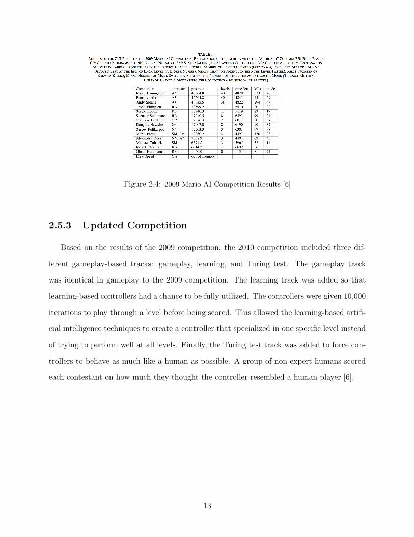
Figure 2.4: 2009 Mario AI Competition Results [6]

2.5.3 Updated Competition

Based on the results of the 2009 competition, the 2010 competition included three dif-

ferent gameplay-based tracks: gameplay, learning, and Turing test. The gameplay track

was identical in gameplay to the 2009 competition. The learning track was added so that

learning-based controllers had a chance to be fully utilized. The controllers were given 10,000

iterations to play through a level before being scored. This allowed the learning-based artifi-

cial intelligence techniques to create a controller that specialized in one specific level instead

of trying to perform well at all levels. Finally, the Turing test track was added to force con-

trollers to behave as much like a human as possible. A group of non-expert humans scored

each contestant on how much they thought the controller resembled a human player [6].

13

3 Methodology

We used the results of the Mario AI competitions as a benchmark to test EBTs and

NEAT. This software was created by Sergey Karakovskiy and Julian Togelius for the 2012

Mario AI competition. It provided the interface to an instance of Super Mario Bros. which

allowed us to obtain information about Mario’s current power-up state, the state of the

current 21× 21 tile screen, and the location of all on-screen enemies.

3.1 Mario Level Parameters

Mario started each level with the fire flower power-up, adhering to the level design used

in the 2010 Mario AI competition [6]. This allowed our AI controller to use the fire flower

ability to easily defeat enemies and take up to three hits before dying. Levels included the

basic enemy types along with pits and various platforms. In addition, a small number of

levels had increased difficulty by utilizing advanced enemy types, such as flying Goombas

and Koopas, and larger pits to jump over.

3.1.1 Training Levels

We trained each AI on a total of 25 different levels. These levels consist of 20 difficulty

0 levels and five difficulty 1 levels. The difficulty 0 levels represented the level of challenge

present in the actual Super Mario Bros. game. The difficulty 1 levels were significantly

more difficult than the difficulty 0 levels and contained more enemies and more challenging

terrain. Since there were 25 levels, the maximum possible fitness was 102,400.

14

3.1.2 Test Levels

To test the effectiveness of each type of AI controller, we tested the champion of genera-

tion 1000 on a series of levels that were not part of the training levels. This test judged how

well the AI controllers could generalize to levels they hadn’t seen before. This also tested to

see if the AI controller became overfit to the training levels.

3.2 AI Controller Parameters

3.2.1 Evolution Process

Each AI evolved in populations of 100 chromosomes. There were a total of 1000 genera-

tions for each evolution process. The chromosome with the highest fitness for each generation

was saved as the champion of that generation.

3.2.2 Evaluating Fitness of Controllers

We evaluated the fitness of our artificial intelligence controllers by measuring the total

distance traveled by Mario across the test levels. Each level was 4096 units long, so the

maximum possible fitness for n levels was 4096 · n. This was the same metric used in the

2012 Mario AI competition [6]. If there were multiple controllers with the same fitness, the

AI chose the controller with the smallest number of genomes.

3.2.3 Feature Sets

We tested three different feature sets. Each feature set provided the AI controller with

information about Mario’s surroundings within a given radius, as seen in Figure 3.1. The

three radii being tested were 1, 2, and 3, resulting in inputs of 3 × 3, 5 × 5, and 7 × 7

blocks, respectively. For each block within the radius, the AI controller was given two

pieces of information. The first indicated if there was a block in that position, and the

15

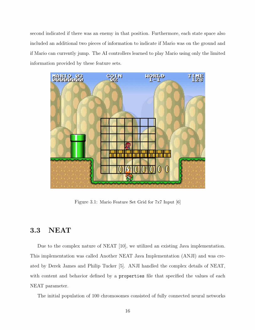
second indicated if there was an enemy in that position. Furthermore, each state space also

included an additional two pieces of information to indicate if Mario was on the ground and

if Mario can currently jump. The AI controllers learned to play Mario using only the limited

information provided by these feature sets.

Figure 3.1: Mario Feature Set Grid for 7x7 Input [6]

3.3 NEAT

Due to the complex nature of NEAT [10], we utilized an existing Java implementation.

This implementation was called Another NEAT Java Implementation (ANJI) and was cre-

ated by Derek James and Philip Tucker [5]. ANJI handled the complex details of NEAT,

with content and behavior defined by a properties file that specified the values of each

NEAT parameter.

The initial population of 100 chromosomes consisted of fully connected neural networks

16

with no hidden neurons. Each neural network started with 6 output neurons and between

20 and 100 input neurons based on the feature set. The weight of each connection was a

random real number. At each generation, the fitness of each chromosome was calculated

and a new generation was created based upon the specified NEAT parameters. These new

chromosomes have updated connection weights and new hidden nodes that were likely to

improve the fitness of the chromosomes.

We utilized the default settings provided by ANJI. These defaults included an add con-

nection rate of 1%, an add neuron rate of 0.5%, a weight mutation rate of 80%, a survival

rate of 20%, and a speciation threshold of 20%. The defaults provided by ANJI created an

optimal environment for rapid evolution.

3.4 EBT

The AI controllers have six inputs to the running Mario game. These inputs correspond

to the six controller buttons: left, right, up, down, jump, and run/fire. Thus, the output

of the behavior trees was a combination of the six available buttons [7]. The behavior trees

had to take a set of environmental and enemy conditions and select the appropriate action.

Due to this requirement, the EBTs consisted of several types of conditional nodes and one

type of action node.

Conditional Nodes: Conditional nodes create branches in the tree and were based on the

terrain and enemy data point occurring around Mario. This also included if Mario

has the ability to jump and if Mario is currently on the ground. Every block within

Mario’s input radius was checked to see if there was a block or enemy present (Figure

3.1). The EBTs learned how to react in each situation. Each conditional node led to

either another conditional node or the appropriate combination of buttons specified by

an action node (Figure 2.3).

Action Nodes: Leaves in an EBT are known as action nodes. For Mario, these nodes

17

consist of a set of buttons to be pressed. The tree is then reevaluated after a single

frame passes in the Mario game.

We used a context free grammar to encode the EBT as a string of integers. These strings of

integers served as chromosomes in our GA, allowing our EBTs to evolve by swapping portions

of their encoding with portions of other EBTs’ encoding. At the end of each generation,

EBTs were selected for crossover based on their fitness. The higher the fitness, the more likely

they were to participate in crossover. The EBT with the highest fitness for that generation,

known as the “champion”, was carried over, unaltered, to the next generation. Over a large

number of iterations, this led to improvement of the AI controllers and eventually an EBT

that performed well at multiple levels.

Similar to NEAT, we implemented the genetic algorithm with a population size of 100.

We gave these individuals a maximum number of nodes to prevent unnecessary repetition.

The maximum number of nodes was based on the feature set: 200, 300, and 400 for 3×3, 5×5,

and 7 × 7 respectively. Unlike NEAT, we customized the EBT mutation and reproduction

probability to 30% and 10% respectively. Of those selected, the genetic algorithm chose 90%

for crossover and 10% for mutation. We also set the maximum initial depth, or how many

levels the initial trees can have, to eight. We chose these parameters based on a similar

example provided by the Java Genetic Algorithms Package.

We used Java Genetic Algorithms Package (JGAP http://jgap.sourceforge.net/) to define

our conditional and action nodes and run our genetic algorithm. This framework was entirely

written in Java. Overall, JGAP provided a solid foundation that allowed us to focus entirely

on writing our EBT grammar.

3.5 Comparisons

Both the NEAT and EBT algorithms were run with a population size of 100 for 1000

generations, once for each of the three feature sets. We compared them on a number of

18

aspects, including maximum fitness, learning speed, evolution timing, generalization, and

complexity.

Maximum Fitness: The maximum fitness is the fitness of the champion AI from generation

1000.

Rise Time: For these experiments, our rise time was measured as the number of generations

required to reach a fitness of 75%. This measured how quickly a particular algorithm

could achieve an acceptable level of performance.

Evolution Timing Data: The timing data refers to the time necessary for each generation

to evolve. That time is equal to the total time it takes to evaluate each chromosome on

the training levels and perform crossover and mutation to generate a new population.

Different algorithms completed generations at different rates.

Complexity: Complexity refers to the number of genes in a chromosome. In NEAT, the

three types of genes are input nodes, hidden nodes, and output nodes. In EBTs, the

two types of genes are conditional nodes and action nodes. A smaller model size is

easier to evaluate and therefore more desirable.

Generalization: Generalization refers to how well an AI performs on levels that weren’t

included in the training level set. This was measured by the average fitness across the

test level set. AIs are more useful if they can complete levels that they haven’t seen

before.

19

4 Data and Analysis

Over the course of each evolution process, we recorded important values for each gener-

ation, including the champion fitness, the champion complexity, and the time to complete

the last generation. In addition, each champion was evaluated on a set of test levels to get

a better insight into their strengths and weaknesses.

4.1 Training Data

During the training, we kept track of the maximum fitness so that we could compare the

strongest AIs against each other.

20

4.1.1 NEAT

Figure 4.1: NEAT Training Data Results

Figure 4.1, above, shows the maximum fitness of NEAT over the course of 1000 genera-

tions. The graph shows the maximum fitness of each generation for 3× 3, 5× 5, and 7× 7

NEAT implementations in blue, green, and yellow, respectively.

The 3 × 3 was the strongest of the NEAT implementations. It learned the quickest as

shown by generations one through 100. The 3×3 also had the highest performing champion

after 1000 generations.

The 5× 5 was almost as good as the 3× 3 implementation. However, it learned slightly

slower and peaked lower. The 5 × 5 also showed variable maximum fitness unlike most of

the AIs. This is because NEAT is not guaranteed to keep the champion individuals from

generation to generation.

The 7× 7 was stopped at 457 generations due to its memory usage. It showed the worst

21

learning and maximum fitness. However, it was not far from 5×5 and 3×3 implementations.

The computation requirements for the 7 × 7 were simply too high to judge its fitness after

457 generations.

4.1.2 EBT

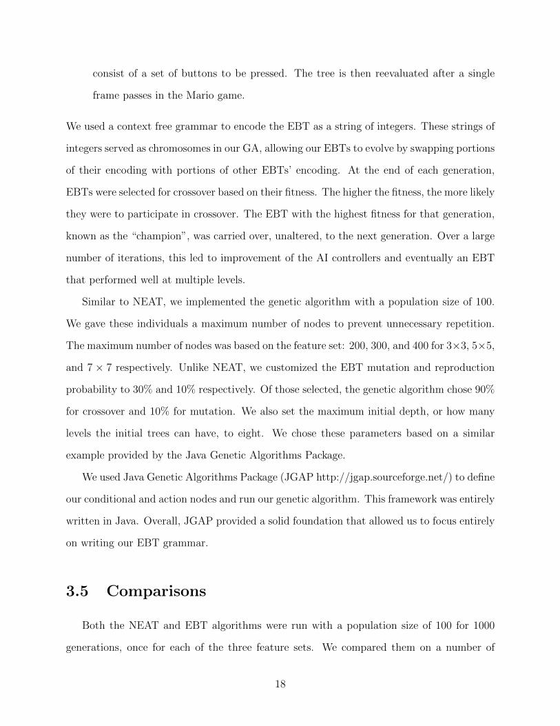
Figure 4.2: EBT Training Data Results

Figure 4.2, above, shows the results of EBT over the course of 1000 generations. The

graph shows the maximum fitness of each generation for 3 × 3, 5 × 5, and 7 × 7 EBT

implementations.

The 3 × 3 had the highest fitness of the EBT implementations. The 5 × 5 showed the

worst learning and had the lowest final fitness. It showed an unique behavior in that it stayed

below 20% fitness for the first 997 generations. Although this seems like an unlikely outcome,

we attempted the 5× 5 EBT implementation many times and ended up with similar results

22

each time, suggesting that the 5× 5 was unable to generalize as well as the 3× 3 or learn as

well as the 7× 7.

The 7× 7 had similar fitness to the 3× 3 implementation. Both of them learned quickly

and both peaked at about the same percentage. This is unusual as the radius in between

them failed to learn as quickly or as well.

4.1.3 Comparisons

Figure 4.3: Maximum Fitness Summary

The maximum fitness of EBTs and NEAT were similar. EBTs achieved a maximum

fitness of 86.1% with the 3×3 feature set while NEAT achieved a maximum fitness of 86.9%

with the 3 × 3 feature set. In contrast, the worst maximum fitness for EBTs was 75.3%

from the 5 × 5 feature set while the worst maximum fitness for NEAT was 81.9% from the

7× 7 feature set. Overall, the 3× 3 NEAT produced the highest maximum fitness of 86.9%,

beating out the 3× 3 EBT by only 0.8%. Thus the difference in maximum fitness between

the NEAT and EBT implementations was negligible.

23

4.2 Rise Time

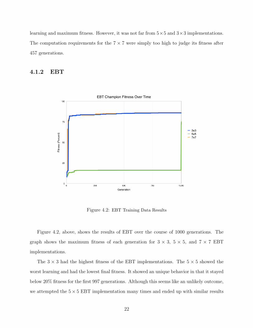
Figure 4.4: Rise Time Summary

The rise time varied significantly between the genetic algorithms and the feature sets.

For the 3 × 3 feature set, both NEAT and EBT had a rise time of 17 generations . Due to

the odd behavior of the 5 × 5 EBT, it had a rise time of 1000 generations while the 5 × 5

NEAT had a rise time of only 61 generations. For the 7 × 7 feature set, NEAT had a rise

time of 128 generations while EBT had a rise time of only 15 generations.

In general, the EBT implementations had a faster learning rate than the corresponding

NEAT implementations. Hence, EBTs are more effective for applications that require fast

learning in a small number of generations.

24

4.3 Evolution Timing Data

Figure 4.5: Evolution Timing Data

For the first 50 generations of each run, each generation took approximately three minutes

to complete chromosome evaluation, crossover, and mutation. Since crossover and mutation

were not computationally expensive, most of the three minutes was spent evaluating each

chromosome on the training level set. However, as each run progressed beyond the first 100

generations, the time to evolve each generation grew. This is because the chromosomes grew

larger over time, so by generation 100, their size started affecting the speed of evaluation,

mutation, and crossover.

For the EBT runs, the time to evolve each generation grew linearly. The 3 × 3 run

progressed from three minutes per generation at the start to about five minutes per generation

at the end. The 5 × 5 run progressed from three minutes per generation to about seven

minutes per generation, and the 7× 7 run progressed from three minutes per generation to

approximately eight minutes per generation. In total, the 3× 3 run took about 21 hours to

finish, the 5× 5 run took 23.5 hours to finish, and the 7× 7 run took 24.5 hours to finish.

The time to evolve each generation of the NEAT runs grew more rapidly than the EBT

runs. This is due to the fact that fully connected neural networks are inherently more

complex than behavior trees, and therefore require more time to process. While each of the

runs began at three minutes per generation, the 3× 3 run ended up taking over 15 minutes

25

per generation by generation 1000, resulting in a total computation time of over 30 hours.

The 5 × 5 run progressed to taking about 25 minutes per generation by the end, resulting

in a total time of 70 hours. By the time that the 7× 7 run ran out of memory, the average

generation took more than 90 minutes per generation to evolve, with a maximum of 122

minutes per generation. In total, the 7 × 7 implementation ran for over ten days before

running out of memory at generation 457.

At the start of each evolution process, both EBT and NEAT took between three to

five minutes to complete a generation. While all of the EBT implementations stayed under

15 minutes per generation throughout the whole process, the NEAT implementations took

upwards of 120 minutes per generation by the end of the evolution process. Therefore, EBT

is the more effective algorithm for applications that require quick results.

26

4.4 Complexity

4.4.1 NEAT

Figure 4.6: NEAT Champion Complexity Over Time

Figure 4.6, above, shows each the champion’s complexity for each generation of the NEAT

evolution process. On average, the complexity increased over time for each input size while

constantly fluctuating. This is indicative of the fact that NEAT divides each population into

species that have different approaches to playing Mario. The champion complexity oscillates

between two or three values, as small improvements are made by competing species, each

with very different structures, but similar fitness.

In addition, the average complexity increased with input size. The maximum complexity

of the 3× 3 was 670, while the maximum complexity of the 5× 5 was 4683. The 7× 7 was

significantly more complex, with a maximum complexity of 14803, despite the fact that it

27

only ran for 457 generations. If the trend continued linearly, the 7 × 7 would have reached

a complexity of over 17000 by generation 1000.

4.4.2 EBT

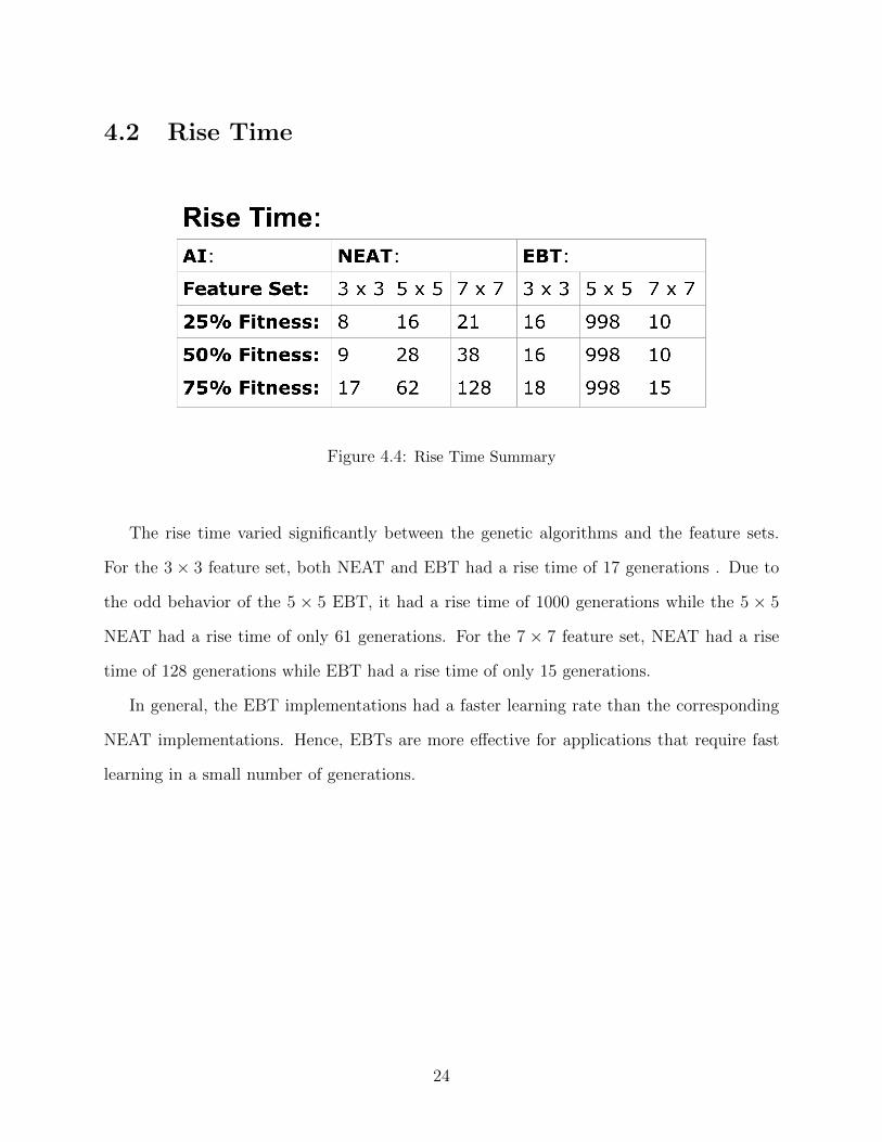
Figure 4.7: EBT Champion Complexity Over Time

Figure 4.7, above, shows the champion’s complexity for each generation of the EBT

evolution process. EBTs often generated significant repetition throughout the evolution

process. To help focus the evolution process, each input size was given a limit on the

number of genes in its EBTs. These limits were chosen to reduce repetition while still

allowing complex solutions to form. The 3× 3 had a limit of 200 genes, the 5× 5 had a limit

of 300 genes, and the 7× 7 had a limit of 400 genes.

During each evolution process, the average complexity quickly rose to the gene limit and

fluctuated around that limit. This behavior was expected and often resulted in a series of

28

champions that had the same fitness but different complexity. For example, the champions

of generation 820 and generation 998 for the 3 × 3 both had a fitness of 85.8%. However,

the champion of generation 820, as seen in Figure 4.8, had a complexity of 49 while the

champion of generation 998, as seen in Figure 4.9, had a complexity of 191.

Figure 4.8: 3× 3 EBT from Generation 820

Figure 4.9: 3× 3 EBT from Generation 998

29

4.4.3 Comparisons

Because the EBTs were limited to a set number of genes, the EBTs ended up with

a much lower complexity than the corresponding NEAT implementations. However, even

without the limit in place, the EBTs that were generated were less complex than the NEAT

equivalents. This is because a fully connected neural network is inherently more complex

than a behavior tree. Therefore, given two AIs of equal fitness, the EBT AI will likely be

less complex than the NEAT AI.

4.5 Test Data

The final champion of each feature set was tested against a series of previously unseen

levels to more accurately test its ability to generalize to new Mario levels. Due to the fact

that the training levels consisted of difficulty 0 and difficulty 1 levels, the test levels consisted

of 1000 difficulty 0 levels and 1000 difficulty 1 levels.

30

4.5.1 Difficulty 0 Test Levels

Figure 4.10: NEAT vs. EBT Difficulty 0 Test Level Fitness

Figure 4.10, above, shows the average fitness of each champion for the 1000 difficulty 0

test levels. In addition, it also includes error bars to demonstrate the wide range of skill

levels across different levels in the test level set.

In general, the 3 × 3 of each method performed better than the 5 × 5, which in turn

performed better than the corresponding 7 × 7. We observed this in the training data as

well, but the test level data highlights the true difference in fitness between each champion.

While Figure 4.10 shows the average fitness across all 1000 levels, that metric doesn’t

necessarily show how many individual levels each champion fully completed. Therefore,

Figure 4.11 shows the percentage of levels that each champion fully completed.

31

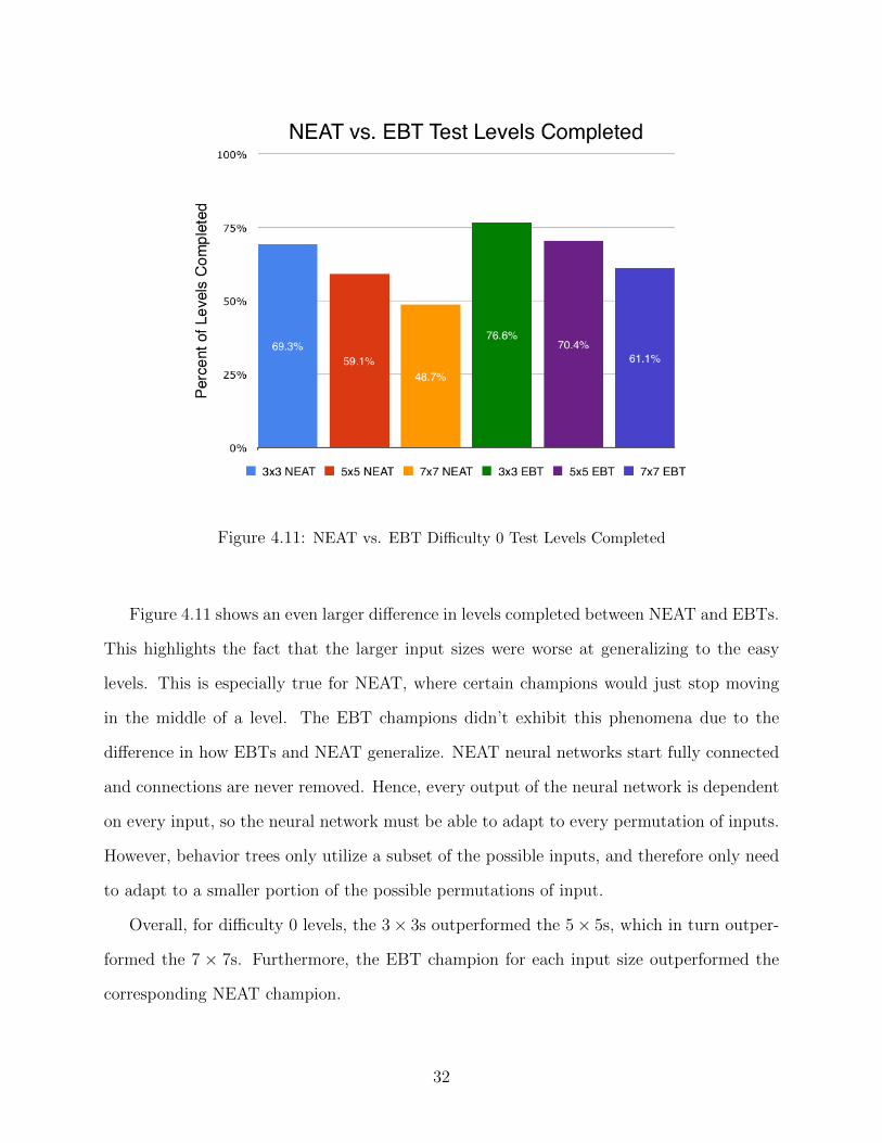
Figure 4.11: NEAT vs. EBT Difficulty 0 Test Levels Completed

Figure 4.11 shows an even larger difference in levels completed between NEAT and EBTs.

This highlights the fact that the larger input sizes were worse at generalizing to the easy

levels. This is especially true for NEAT, where certain champions would just stop moving

in the middle of a level. The EBT champions didn’t exhibit this phenomena due to the

difference in how EBTs and NEAT generalize. NEAT neural networks start fully connected

and connections are never removed. Hence, every output of the neural network is dependent

on every input, so the neural network must be able to adapt to every permutation of inputs.

However, behavior trees only utilize a subset of the possible inputs, and therefore only need

to adapt to a smaller portion of the possible permutations of input.

Overall, for difficulty 0 levels, the 3× 3s outperformed the 5× 5s, which in turn outper-

formed the 7 × 7s. Furthermore, the EBT champion for each input size outperformed the

corresponding NEAT champion.

32

4.5.2 Difficulty 1 Test Levels

Figure 4.12: NEAT vs. EBT Difficulty 1 Test Level Fitness

Figure 4.12, above, shows the average fitness of each champion over 1000 difficulty 1 test

levels.

In general, the performance across difficulty 1 levels was significantly worse than the per-

formance across difficulty 0 levels. For the EBT champions, the larger input sizes performed

better than the smaller input sizes. While this trend doesn’t apply to the NEAT champions,

it is possible that it would if the 7× 7 run had a chance to make it past generation 457.

Out of all 1000 difficulty 1 levels, only one champion managed to complete a single level

in its entirety. That champion was the 7 × 7 EBT and it managed to complete the level

with seed 745. Based on this fact and the trends observed in Figure 4.12, it is evident that

larger input sizes have an advantage in more difficult levels where larger groups of enemies

and more difficult terrain is present.

33

4.6 Generalization

The ability for each champion AI controller to generalize was measured by their average

fitness on the series of test levels and by their ability to perform competently on levels that

they couldn’t complete.

For the difficulty 0 test levels, the EBT champions generalized better than the NEAT

champions. The EBT champions achieved 2.2% to 5.7% higher fitness than their correspond-

ing NEAT champions. In addition, there were locations in the test levels where the NEAT

champions would get stuck and no longer proceed, despite the fact that those locations posed

very little challenge. For example, Figure 4.13 shows where the 7 × 7 NEAT champion got

stuck on the test level with seed 32. At 6% of the way through the level, the 7 × 7 NEAT

champion decided to stay crouched on a block and remain that way until time ran out.

Figure 4.13: 7× 7 NEAT Champion Stuck on Level Seed 32

34

For the difficulty 1 test levels, the clear winner was the 7 × 7 EBT. While the 3 × 3

and 5 × 5 NEAT champions outperformed the corresponding EBT champions, the 7 × 7

outperformed every other champion by at least 4.1%. In addition, the issue of getting stuck

part way through the level wasn’t as big of an issue for the difficulty 1 levels as it was for

the difficulty 0 levels. This was because most of the champions died well before they could

get stuck. Overall, the smaller input sizes outperformed the larger input sizes on difficulty 0

levels, while the reverse was true on the difficulty 1 levels. The 3×3 feature set was great at

generalizing to unseen easy levels, while the 7×7 feature set excelled at adapting to complex

situations in the difficult levels.

35

5 Recommendations

5.1 When to use NEAT

NEAT’s biggest strength is maximum fitness. NEAT showed a slightly higher maximum

fitness of 86.9% as opposed to EBTs maximum fitness of 86.1%. However, in most situations,

an increase of 0.8% maximum fitness is not worth the huge increase in evolution and rise

time. In addition, NEAT’s inability to generalize effectively negates its maximum fitness

advantage. Therefore, NEAT should only be used when extreme amounts of computational

power can be used to evolve NEAT with a large training set over thousands of generations

to make effective use of its maximum fitness advantage.

5.2 When to use EBTs

EBTs were stronger than NEAT at all aspects of the evolution process except for max-

imum fitness. They generalized better, completed the evolution process faster, and had a

higher learning speed. These strengths make EBTs better when time and processing power

are limitations. EBT and NEAT also showed similar maximum fitness, only separated by

.8%. Furthermore, EBTs are human readable, as shown in Figure 2.3, while neural networks

are not. Due to all these strengths, EBTs are better for the majority of situations.

36

6 Areas for Future Work

6.1 New Features

This paper only covered the results of 3× 3, 5× 5, and 7× 7 implementations. However,

other feature sets could be constructed that may produce better results. Instead of using

grid based features, one could implement a radial search for enemies or terrain. One could

also group locations based on their distance from Mario. Locations close to Mario would be

treated like they were in the 3× 3 feature set, while further away locations may be grouped

together to reduce the total number of features. This could help the AI prioritize the features

of nearby locations while still being aware of far away terrain and enemies.

6.2 Improved Training Levels

Due to restrictions in computation power and time, we used a total of 25 training levels

to train the AIs. However, by increasing the number and variety of training levels, one could

produce an AI that not only generalizes better, but also can complete more difficult levels.

There are a total of nine difficulty settings and three level themes that are available for use

in the Mario level generation framework. The higher difficulty settings introduce new enemy

types, such as spiky shell Koopas, that pose a greater challenge for the AI controller. In

addition, the other level themes introduce new types of terrain challenges, such as locations

that require backtracking to proceed.

37

6.3 Other AI Techniques

This paper covered NEAT and EBTs, but there are many other types of AIs capable of

playing Super Mario Bros. There were a number of AIs used during the Super Mario Bros.

competitions including: A*, Q-Learning, and syntax trees. One could compare any of these

AIs along with NEAT and EBTs.

38

7 Conclusion

Both NEAT and EBTs were capable of producing an AI that could complete a variety

of Super Mario Bros. levels. Each genetic algorithm excelled in certain comparison metrics

while falling short in others. The results showed that NEAT had a slightly higher maximum

fitness while performing poorly in all other comparisons. EBTs performed strongly in all

other comparisons, including rise time, evolution time, generalization, and complexity. Due

to how small the difference in maximum fitness between NEAT and EBTs was, we concluded

that EBT is the stronger genetic algorithm for playing Super Mario Bros.

39

Glossary

AI Artificial Intelligence

BT Behavior Tree

CFG Context-free Grammar

EA Evolutionary Algorithm

EBT Evolving Behavior Tree

EBTs Evolving Behavior Trees

JGAP Java Genetic Algorithms Package

GA Genetic Algorithm

GP Genetic Programming

NEAT NeuroEvolution of Augmenting Topologies

40

Bibliography

[1] N. Barricelli. Numerical testing of evolution theories. Acta Biotheoretica, 16(1-2):69–98,

1962.

[2] M. Booth. The ai systems of left 4 dead. In Artificial Intelligence and Interactive Digital

Entertainment Conference (Stanford University). Valve Software, 2009.

[3] S. Chernova. Artificial neural networks. 2014.

[4] J. J. Grefenstette and N. L. Cramer. Proceedings of an international conference on ge-

netic algorithms and their applications. held at Carnegie-Mellon University, Pittsburgh,

Pa, 1985.

[5] D. James and P. Tucker. Another neat java implementation, Aug. 2005.

[6] S. Karakovskiy and J. Togelius. The mario ai benchmark and competitions. Computa-

tional Intelligence and AI in Games, IEEE Transactions on, 4(1):55–67, 2012.

[7] N. of America. Super Mario Bros. Instruction Booklet. Nintendo, Redmond, WA, first

edition, 1988.

[8] D. Perez, M. Nicolau, M. ONeill, and A. Brabazon. Evolving behaviour trees for the

mario ai competition using grammatical evolution. In Applications of Evolutionary

Computation, pages 123–132. Springer, 2011.

[9] H. Rowley, S. Baluja, and T. Kanade. Neural network-based face detection. Pattern

Analysis and Machine Intelligence, IEEE Transactions on, 20(1):23–38, Jan 1998.

[10] K. O. Stanley and R. Miikkulainen. Evolving neural networks through augmenting

topologies. Evolutionary Computation, 10(2):99–127, 2002.

41

[11] J. Togelius, S. Karakovskiy, and R. Baumgarten. The 2009 mario ai competition. In

Evolutionary Computation (CEC), 2010 IEEE Congress on, pages 1–8. IEEE, 2010.

[12] P. D. Wasserman. Advanced Methods in Neural Computing. John Wiley & Sons, Inc.,

New York, NY, USA, 1st edition, 1993.

[13] D. Whitley. A genetic algorithm tutorial. Statistics and Computing, 4(2):65–85, 1994.

42