A Comparative Study for Single Image Blind Deblurring

Wei-Sheng Lai1 Jia-Bin Huang2 Zhe Hu1 Narendra Ahuja2 Ming-Hsuan Yang1

1University of California, Merced 2University of Illinois, Urbana-Champaign

http://vllab.ucmerced.edu/˜wlai24/cvpr16_deblur_study

Abstract

Numerous single image blind deblurring algorithms

have been proposed to restore latent sharp images under

camera motion. However, these algorithms are mainly eval-

uated using either synthetic datasets or few selected real

blurred images. It is thus unclear how these algorithms

would perform on images acquired “in the wild” and how

we could gauge the progress in the field. In this paper, we

aim to bridge this gap. We present the first comprehensive

perceptual study and analysis of single image blind deblur-

ring using real-world blurred images. First, we collect a

dataset of real blurred images and a dataset of syntheti-

cally blurred images. Using these datasets, we conduct a

large-scale user study to quantify the performance of sev-

eral representative state-of-the-art blind deblurring algo-

rithms. Second, we systematically analyze subject prefer-

ences, including the level of agreement, significance tests of

score differences, and rationales for preferring one method

over another. Third, we study the correlation between hu-

man subjective scores and several full-reference and no-

reference image quality metrics. Our evaluation and anal-

ysis indicate the performance gap between synthetically

blurred images and real blurred image and sheds light on

future research in single image blind deblurring.

1. Introduction

The recent years have witnessed significant progress in

single image blind deblurring (or motion deblurring). The

progress in this field can be attributed to the advancement

of efficient inference algorithms [2, 5, 17, 35, 44], various

natural image priors [15, 21, 29, 38, 45], and more general

motion blur models [8, 9, 11, 43]. To quantify and compare

the performance of competing algorithms, existing meth-

ods either use (1) synthetic datasets [17, 38] with uniform

blurred images generated by convolving a sharp image with

a known blur kernel, or (2) a non-uniform blurred bench-

mark [13] constructed by recording and playing back cam-

era motion in a lab setting. However, existing datasets do

not consider several crucial factors, e.g., scene depth varia-

tion, sensor saturation and nonlinear camera response func-

Blurred input image Cho & Lee [2] Krishnan et al. [15]

Whyte et al. [43] Sun et al. [38] Xu et al. [45]

Zhong et al. [49] Pan et al. [29] Perrone et al. [31]

Figure 1. A blurred image from the real dataset proposed in this

work and a few deblurred results from state-of-the-art algorithms,

where there is no clear winner. In this work, we aim to evaluate

the performance of single image deblurring algorithms on the real-

world blurred images by human perceptual studies.

tions in a camera pipeline. To understand the true progress

of deblurring algorithms, it is important to evaluate the per-

formance “in the wild”. While several work has reported

impressive results on real blurred images, the lack of a

large benchmark dataset and perceptual comparison makes

it impossible to evaluate the relative strengths of these algo-

rithms in the literature.

There are two main drawbacks in existing evaluation ap-

proaches. First, the synthetically generated blurred images

often fail to capture the complexity and the characteristics

of real motion blur degradation. For example, the camera

motion has 6 degrees of freedom (3 translations and 3 rota-

tions) while a convolution model considers only 2D trans-

lations parallel to the image plane [17, 38]. Lens distortion,

sensor saturation, nonlinear transform functions, noise, and

compression in a camera pipeline are also not taken into ac-

count in these synthetically generated images. Furthermore,

the constant scene depth assumption in a convolution model

and the non-uniform blurred benchmark [13] may not hold

in many real scenes where the depth variation cannot be ne-

glected. Evaluations on these datasets do not reflect the per-

formance of single image blind deblurring algorithms on the

11701

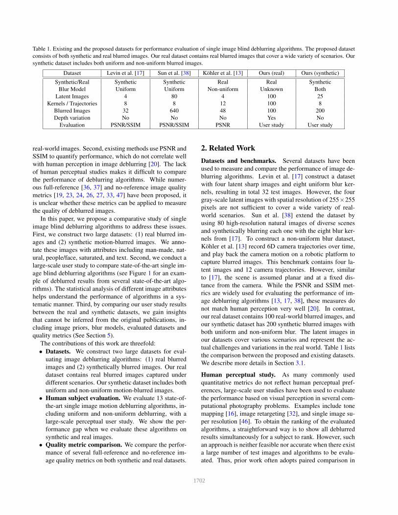
Table 1. Existing and the proposed datasets for performance evaluation of single image blind deblurring algorithms. The proposed dataset

consists of both synthetic and real blurred images. Our real dataset contains real blurred images that cover a wide variety of scenarios. Our

synthetic dataset includes both uniform and non-uniform blurred images.

Dataset Levin et al. [17] Sun et al. [38] Kohler et al. [13] Ours (real) Ours (synthetic)

Synthetic/Real Synthetic Synthetic Real Real Synthetic

Blur Model Uniform Uniform Non-uniform Unknown Both

Latent Images 4 80 4 100 25

Kernels / Trajectories 8 8 12 100 8

Blurred Images 32 640 48 100 200

Depth variation No No No Yes No

Evaluation PSNR/SSIM PSNR/SSIM PSNR User study User study

real-world images. Second, existing methods use PSNR and

SSIM to quantify performance, which do not correlate well

with human perception in image deblurring [20]. The lack

of human perceptual studies makes it difficult to compare

the performance of deblurring algorithms. While numer-

ous full-reference [36, 37] and no-reference image quality

metrics [19, 23, 24, 26, 27, 33, 47] have been proposed, it

is unclear whether these metrics can be applied to measure

the quality of deblurred images.

In this paper, we propose a comparative study of single

image blind deblurring algorithms to address these issues.

First, we construct two large datasets: (1) real blurred im-

ages and (2) synthetic motion-blurred images. We anno-

tate these images with attributes including man-made, nat-

ural, people/face, saturated, and text. Second, we conduct a

large-scale user study to compare state-of-the-art single im-

age blind deblurring algorithms (see Figure 1 for an exam-

ple of deblurred results from several state-of-the-art algo-

rithms). The statistical analysis of different image attributes

helps understand the performance of algorithms in a sys-

tematic manner. Third, by comparing our user study results

between the real and synthetic datasets, we gain insights

that cannot be inferred from the original publications, in-

cluding image priors, blur models, evaluated datasets and

quality metrics (See Section 5).

The contributions of this work are threefold:

• Datasets. We construct two large datasets for eval-

uating image deblurring algorithms: (1) real blurred

images and (2) synthetically blurred images. Our real

dataset contains real blurred images captured under

different scenarios. Our synthetic dataset includes both

uniform and non-uniform motion-blurred images.

• Human subject evaluation. We evaluate 13 state-of-

the-art single image motion deblurring algorithms, in-

cluding uniform and non-uniform deblurring, with a

large-scale perceptual user study. We show the per-

formance gap when we evaluate these algorithms on

synthetic and real images.

• Quality metric comparison. We compare the perfor-

mance of several full-reference and no-reference im-

age quality metrics on both synthetic and real datasets.

2. Related Work

Datasets and benchmarks. Several datasets have been

used to measure and compare the performance of image de-

blurring algorithms. Levin et al. [17] construct a dataset

with four latent sharp images and eight uniform blur ker-

nels, resulting in total 32 test images. However, the four

gray-scale latent images with spatial resolution of 255×255

pixels are not sufficient to cover a wide variety of real-

world scenarios. Sun et al. [38] extend the dataset by

using 80 high-resolution natural images of diverse scenes

and synthetically blurring each one with the eight blur ker-

nels from [17]. To construct a non-uniform blur dataset,

Kohler et al. [13] record 6D camera trajectories over time,

and play back the camera motion on a robotic platform to

capture blurred images. This benchmark contains four la-

tent images and 12 camera trajectories. However, similar

to [17], the scene is assumed planar and at a fixed dis-

tance from the camera. While the PSNR and SSIM met-

rics are widely used for evaluating the performance of im-

age deblurring algorithms [13, 17, 38], these measures do

not match human perception very well [20]. In contrast,

our real dataset contains 100 real-world blurred images, and

our synthetic dataset has 200 synthetic blurred images with

both uniform and non-uniform blur. The latent images in

our datasets cover various scenarios and represent the ac-

tual challenges and variations in the real world. Table 1 lists

the comparison between the proposed and existing datasets.

We describe more details in Section 3.1.

Human perceptual study. As many commonly used

quantitative metrics do not reflect human perceptual pref-

erences, large-scale user studies have been used to evaluate

the performance based on visual perception in several com-

putational photography problems. Examples include tone

mapping [16], image retargeting [32], and single image su-

per resolution [46]. To obtain the ranking of the evaluated

algorithms, a straightforward way is to show all deblurred

results simultaneously for a subject to rank. However, such

an approach is neither feasible nor accurate when there exist

a large number of test images and algorithms to be evalu-

ated. Thus, prior work often adopts paired comparison in

1702

(a) man-made (b) man-made, saturated (c) natural (d) natural, saturated (e) people/face (f) text

Figure 2. Sample images with the annotated attributes in our real dataset. The numbers of images belonging to each attribute in our real

dataset are: man-made (66), natural (14), people/face (12), saturated (28), and text (17).

a user study, where subjects are asked to choose a pref-

erence between two results (i.e., partial order), instead of

giving unreliable scores or rankings for comparing multi-

ple results. We note that Liu et al. [20] also conduct a user

study to obtain subjective perceptual scores for image de-

blurring. Our work differs from [20] in three major aspects.

First, the goal of [20] is to learn a no-reference metric from

the collected perceptual scores while our objective is the

performance comparison of state-of-the-art deblurring algo-

rithms on the real-world images. Second, unlike [20] where

synthetic uniform blurred images are used, our real dataset

better reflects the complexity and variations of blurred im-

ages in the real world. Third, we evaluate both uniform and

non-uniform deblurring algorithms while the focus of [20]

is on algorithms addressing uniform blur only.

3. Experimental Settings

3.1. Image Datasets

Real image dataset. In this paper, we aim to evaluate

the performance of deblurring algorithms for real blurred

images “in the wild”. To this end, we construct a set of

100 real blurred images via multiple sources, e.g., repre-

sentative images from previous work [2, 5, 43, 44], im-

ages from Flickr and Google Image Search, or pictures cap-

tured by ourselves. All these blurred images are captured in

the real-world scenarios from different cameras (e.g., con-

sumer cameras, DSLR, or cellphone cameras), different set-

tings (e.g., exposure time, aperture size, ISO), and different

users. We categorize images according to the following five

attributes: man-made, natural, people/face, saturated, and

text. Figure 2 shows sample images along with these main

attributes. To make these images computationally feasible

for most deblurring algorithms, we resize each image such

that the maximum dimension is less than 1200 pixels.

Synthetic dataset. To examine the performance consis-

tency between real and synthetic images, we collect 25

sharp images from the Internet as ground truth and synthe-

size 100 non-uniform and 100 uniform blurred images. We

label these images using the above-mentioned five attributes

with each group having at least five images. To synthesize

non-uniform blurred images, we record the 6D camera tra-

jectories using a cellphone with inertial sensors (gyroscope

and accelerometer), and construct a collection of spatially

varying blur kernels by assuming constant depth for the

scenes. We obtain the 100 non-uniform blurred images by

applying four camera trajectories to 25 latent images and

adding 1% Gaussian noise to simulate camera noise. As

the sizes of local blur kernels are less than 25 × 25, we

set the support size to 25× 25 when deblurring those non-

uniform blurred images. For uniform blur, the eight blur

kernels provided by Levin et al. [17] have been used in sev-

eral datasets [28, 29, 38]. However, the maximum blur ker-

nel size of these eight blur kernels is 41×41, which is rel-

atively small in the real-world cases. We thus use the al-

gorithm in [34] to synthesize blur kernels by sampling ran-

dom 6D camera trajectories, generating four uniform blur

kernels with size ranging from 51× 51 to 101× 101. We

then use a convolution model with 1% Gaussian noise to

synthesize the 100 uniform blurred images. We present our

uniform and non-uniform blur kernels in the supplementary

material. We create the synthetic saturated images in a way

similar to [3, 10]. Specifically, we first stretch the inten-

sity range of the latent image from [0,1] to [−0.1,1.8], and

convolve the blur kernels with the images. We then clip the

blurred images into the range of [0,1]. The same process is

adopted for generating non-uniform blurred images.

3.2. Evaluated Algorithms

We evaluate deblurring algorithms with publicly avail-

able source code or binary executable. We evaluate 13 rep-

resentative state-of-the-art algorithms [2, 5, 15, 18, 21, 29,

31, 38, 43, 44, 45, 48, 49] in our experiments1. We include

the input blurred images in the evaluation as well. Table 2

shows the list of evaluated algorithms.

We fix the support size of the blur kernel for each eval-

uated algorithm when estimating a blur kernel from a test

image. For fair comparisons, we use the default param-

eter values and apply the same non-blind deconvolution

method [14] with the estimated kernels to obtain the final

deblurred results. However, the method [14] fails to han-

dle images with large saturated regions. In Figure 3(a),

we show an example where the non-blind deconvolution

1While the method [48] is designed for multi-image blind deconvo-

lution, it can be applied to single images as well. As the non-uniform

method [45] on the project website does not work stably for large blur ker-

nels, we use the uniform deblurring code of [45] requested from the author.

1703

Table 2. List of evaluated algorithms. We present a complete table

with image priors, blur kernel priors and the execution time of all

evaluated algorithms in the supplementary material.

Algorithm Blur Model Algorithm Blur Model

Fergus-06 [5] Uniform Xu-13 [45] Uniform

Cho-09 [2] Uniform Zhang-13 [48] Uniform

Xu-10 [44] Uniform Zhong-13 [49] Uniform

Krishnan-11 [15] Uniform Michaeli-14 [21] Uniform

Levin-11 [18] Uniform Pan-14 [29] Uniform

Whyte-12 [43] Non-uniform Perrone-14 [31] Uniform

Sun-13 [38] Uniform

(a) kernel [29] + nonblind [14] (b) kernel [29] + nonblind [42]

Figure 3. Deblurring saturated images with fast non-blind decon-

volution [14] and non-blind deconvolution with saturation han-

dling [42].

method [14] results in serious ringing artifacts. To ad-

dress this issue, we adopt the non-blind deconvolution algo-

rithm [42] that explicitly handles saturated regions when re-

constructing the test images with this attribute. Figure 3(b)

shows the deblurred result by using [42] for non-blind de-

convolution. We note that the some methods [17, 21, 42, 44]

fail to estimate large blur kernels in about 0.5% of all test

images. We exclude these failure cases from our evaluation.

3.3. Human Subject Study

We conduct our experiments using Amazon Mechanical

Turk for large-scale subject studies to evaluate the perfor-

mance of single image blind deblurring algorithms. We

adopt the paired comparison approach that requires each

human subject to choose a preferred image from a pair of

deblurred images. We design a website that allows each

subject to flip between two deblurred images and easily ex-

amine the differences. We show a screenshot of the user

interface in the supplementary material. There are 14 result

images (13 deblurred images and 1 blurred input) for each

test image in our datasets. The total number of pair com-

parisons is(

142

)

× 100 = 9100. In a user study session, we

ask each subject to compare 50 pairs of images. To remove

careless comparisons by the subjects, we introduce sanity

check by adding several image pairs where one image is

considerably better than the other. For the real dataset, we

manually select some pairs of well-deblurred images and

images containing severe ringing artifacts or noise. For the

synthetic dataset, we use the pairs of ground-truth latent and

blurred images. Among the 50 pairs of images for each

subject, we select 10 pairs for a sanity check. We discard

the voting results by a subject if the subject fails the sanity

check more than once. We collect the results of human sub-

ject studies from 2,100 users. The average time to complete

a survey is 15 minutes. We discard 1.45% of the votes (from

subjects who fail to pass the sanity check).

4. Evaluation and Analysis

In this work, we aim to evaluate the performance of

single image blind deblurring algorithms based on human

visual perception. In addition to ranking the algorithms,

we exploit the correlation between the real and synthetic

datasets, as well as the performance of image quality met-

rics on predicting the quality of deblurred images. First,

we analyze the degree of agreement [12] among subjects to

make sure that the votes are not random. Second, we fit

paired comparison results to the Bradley-Terry model [1] to

obtain a global score and rank for each algorithm. We ana-

lyze the convergence of ranking to show that the number of

votes and images in our human subject study are sufficient

to draw solid conclusions. We also conduct a significance

test [6] to group the evaluated algorithms based on percep-

tual quality (that are statistically indistinguishable). Finally,

we show the correlation between human perceptual scores

and existing image quality metrics.

4.1. Coefficient of Agreement

While we rule out noisy votes with the use of san-

ity check, the votes may appear random if the partici-

pants’ preferences are dramatically different. We thus study

the similarity of choices (i.e., the degree of agreement)

among subjects. We apply the Kendall coefficient of agree-

ment [12] to quantify the level of agreement with u:

u =2W

(

S2

)(

M2

) −1, W = ∑i6= j

(

ci j

2

)

, (1)

where ci j is the number of times that method i is chosen over

method j, S denotes the number of subjects, and M repre-

sents the number of compared methods. If all subjects make

the same choice for each comparison, then the Kendall co-

efficient of agreement u is equal to 1. The minimum value

of u is −1/S, indicating evenly distributed answers. For

example, suppose that there are 100 subjects answering one

binary preference question (choice of A or B, assuming A is

better than B). The Kendall coefficient of agreement u= 0.1if there are 67 subjects choosing A over B, and u = 0.2 if

there are 73 subjects choosing A over B. If 50 subjects vote

for A and 50 subjects vote for B, u attains the minimum

value of −0.01.

In our evaluation, we randomly select pairs of deblurred

images and ask the subjects’ preference. As a result, we

balance the subject votes by uniformly sampling the paired

comparisons so that all the evaluated methods are compared

at the same frequency. In Figure 4, we show the Kendall

coefficients of the agreement under different attributes. The

1704

00.05

0.10.15

0.20.25

0.30.35

0.40.45

man-made natural people/face saturated text all

Kendall Coefficient of Agreement

Synthetic (uniform) Synthetic (non-uniform) Real

Figure 4. Kendall coefficient of agreement under different at-

tributes in our human subject study.

coefficients for both the real and the synthetic non-uniform

datasets are all around 0.12. On the other hand, we observe

a higher level of agreement for the synthetic uniform dataset

(u = 0.26).

We note that many algorithms (e.g., [2, 17, 21, 48]) fa-

vor no-blur explanations for the test images in the synthetic

non-uniform dataset. In such cases, subjects have to choose

between two poorly deblurred images, which leads to incon-

sistent votes. For real blurred images, many factors (e.g.,

depth variation, nonlinear camera response functions, and

unknown camera noise) affect the performance of deblur-

ring algorithms. Existing algorithms often have difficulty

in handling real blurred images as they do not take these

factors into considerations. In many test images, there is no

clear winner. As a result, the degree of agreement in the real

dataset is relatively low. We observe that the coefficients of

agreement for text images on both the real and the synthetic

datasets are higher than other attributes. One possible rea-

son is that human subjects prefer sharp text images (as they

are easier to read). The high contrast of the deblurred text

images makes the comparisons less ambiguous.

4.2. Global Ranking

To compute the global ranking from paired comparisons,

we use the Bradley-Terry model (B-T model) [1]: a prob-

ability model that predicts the outcome of the paired com-

parison. We denote s = [s1,s2, · · · ,sM] as M scores of the

evaluated methods. The B-T model assumes that the proba-

bility of choosing method i over method j is:

pi j =esi

esi + es j. (2)

Since each pair of result (i, j) is compared by multiple sub-

jects, the likelihood of i over j is defined as pci j

i j , where ci j

is the number of times that method i is chosen over method

j. The likelihood of all (i, j) pairs is:

P =M

∏i=1

M

∏j=1j 6=i

pci j

i j . (3)

We can estimate the score si by minimizing the negative log

likelihood of (3):

L(s) =M

∑i=1

M

∑j=1j 6=i

ci j log(esi + es j)−M

∑i=1

M

∑j=1j 6=i

ci jsi. (4)

We can easily solve the optimization problem by setting the

derivative of (4) to zero. We note that there is an ambiguity

in the computed scores s that cannot be determined by solv-

ing (4). That is, adding a constant δ to all si does not change

the objective value. Thus, we normalize the B-T scores by

shifting the scores to zero mean after solving (4).

Ranking. We rank the evaluated methods by the average

B-T scores, and plot the cumulative frequency of B-T scores

in Figure 5. We show the complete ranking results on dif-

ferent attributes in the supplementary material. In Figure 5,

the method with the rightmost curve has a better overall

performance because it has more images with higher B-T

scores. In addition to the performance evaluation, we an-

alyze the correlation of B-T scores between each pair of

datasets as shown in Figure 6. The performance of those

methods located in the lower-right corner of the figure is

over-estimated on the dataset shown on the x-axis. On the

other hand, the performance of those methods located in the

upper-left corner is under-estimated. Take Figure 6(a) as an

example. The methods [38, 44, 45] outperform all the other

algorithms on the synthetic uniform dataset. However, their

performances on the real dataset are not as competitive, e.g.,

the results from [29, 15] achieves higher scores than that

of [38, 44, 45]. In this case, performance of [38, 44, 45]

is over-estimated and the performance of [29, 15] is under-

estimated on the synthetic uniform dataset. Therefore, the

evaluation results based on synthetic uniform images do

not well reflect the performance on the real-world images.

In Figure 6(b), we observe that the performance of deblur-

ring algorithms are similar on the real and the synthetic non-

uniform datasets.

Convergence analysis. We analyze the convergence of

global ranking on (1) the number of subject votes and (2)

the number of test images to ensure that the number of votes

and images are sufficiently large for performance evalua-

tion. We randomly sample k = 500,1000,2000,3000,4000

votes from a total of 23,478 voting results in the real dataset

and compute the B-T scores for each evaluated algorithm.

We repeat this process 1000 times with different sample of

votes. Figure 7(a) shows the mean and standard deviation

for each k. At the beginning (k = 500), the error bars of

these methods overlap with each other. When k ≥ 2000, the

standard deviations become sufficiently small, and the B-T

scores of each method converge.

We conduct a similar analysis regarding the number of

images. We randomly sample k (k = 5,10,20,30,40) im-

ages out of a total of 100 images from our real dataset,

1705

B-T Scores-5 0 5

Cum

ulat

ive

Freq

uenc

y

0

0.2

0.4

0.6

0.8

1Real (all)

Pan-14Xu-10Krishnan-11Sun-13Xu-13Whyte-12Cho-09

B-T Scores-5 0 5

Cum

ulat

ive

Freq

uenc

y

0

0.2

0.4

0.6

0.8

1Uniform (all)

Xu-10Sun-13Xu-13Pan-14Perrone-14Zhong-13Michaeli-14

B-T Scores-5 0 5

Cum

ulat

ive

Freq

uenc

y

0

0.2

0.4

0.6

0.8

1Non-Uniform (all)

Pan-14Perrone-14Xu-10Xu-13Krishnan-11Sun-13Zhong-13

(a) Real dataset (b) Synthetic (uniform) dataset (c) Synthetic (non-uniform) dataset

Figure 5. Cumulative frequency of B-T scores for each dataset. We normalize the frequency such that the maximum frequency is equal to

1. The method whose curve locates at right has more images with higher scores, which stands for better overall performance. Only the top

7 methods are presented for clarity. The complete plots of all evaluated methods are illustrated in the supplementary material.

Xu-10Blur Fergus-06 Cho-09 Krishnan-11 Levin-11 Whyte-12 Xu-13Sun-13 Zhang-13 Zhong-13 Michaeli-14 Pan-14 Perrone-14

Synthetic Dataset (Uniform)-2 -1 0 1 2

Rea

l Dat

aset

-2

-1

0

1

2

Synthetic Dataset (Non-uniform)-2 -1 0 1 2

Rea

l Dat

aset

-2

-1

0

1

2

Synthetic Dataset (Uniform)-2 -1 0 1 2

Synt

hetic

Dat

aset

(Non

-uni

form

)

-2

-1

0

1

2

(a) (b) (c)

Figure 6. Correlation of B-T scores between a pair of datasets. The performance of those methods located in the lower-right is over-

estimated on the dataset shown on the x-axis, while the performance of the methods located in the upper-left is under-estimated.

Xu-13Pan-14 Zhang-13Perrone-14 BlurKrishnan-11

0 1000 2000 3000 4000Number of Votes

-1.5

-1

-0.5

0

0.5

1

1.5

B-T

Sco

res

0 10 20 30 40Number of Images

-1.5

-1

-0.5

0

0.5

1

1.5

B-T

Sco

res

(a) (b)Figure 7. Convergence analysis on B-T scores with respect to the

number of votes and the number of images.

and then plot the means and the standard deviations in Fig-

ure 7(b). The error-bars become sufficiently small to sep-

arate each evaluated method after using 30 images. These

two experiments demonstrate that the number of votes and

the number of test images are indeed sufficient to obtain

stable scores or ranks.

4.3. Significance Test

An algorithm having a higher B-T score does not mean

that it always outperforms others. To investigate whether

the results of the evaluated methods are statistically dis-

tinguishable, we conduct the significance test [6] for each

dataset. Specifically, we group the evaluated methods if

the difference of obtained votes between any two methods

within a group is less than a threshold.

Pan-14

Sun-13

Whyte-12

Perrone-14

Xu-13

Michaeli-14

Krishnan-11

Xu-10

Cho-09

Zhong-13

Levin-11

Zhang-13

Fergus-06

Blur

(a) Real

Xu-10

Zhong-13

Michaeli-14

Sun-13

Perrone-14

Zhang-13

Xu-13

Pan-14

Whyte-12

Krishnan-11

Cho-09

Levin-11

Blur

Fergus-06

(b) Uniform

Pan-14

Sun-13

Whyte-12

Perrone-14

Xu-13

Michaeli-14

Krishnan-11

Xu-10

Cho-09

Zhong-13

Levin-11

Zhang-13

Fergus-06

Blur

(c) Non-uniform

Figure 8. Grouping of algorithms by the significance test. Algo-

rithms within the same circle have statistically indistinguishable

scores, i.e., the performance is similar.

We denote the difference of the number of votes within a

group of methods as R. We aim to find a threshold R′ such

that the probability P[R ≥ R′] ≤ α , where α is the signifi-

cance level (α = 0.01 in this work). Since the distribution

of R is asymptotically equivalent to the distribution of the

variance-normalized range Wt [7], we can use the following

1706

Blur Fergus-06 Cho-09 Xu-10 Krishnan-11 Levin-11 Whyte-12

Sun-13 Xu-13 Zhang-13 Zhong-13 Michaeli-14 Pan-14 Perrone-14

02468101214

Percentage

Real (saturated)

02468101214

Percentage

Real (text)

02468101214

Percentage

Real (all)

02468101214

Percentage

Uniform (saturated)

02468101214

Percentage

Uniform (text)

02468101214

Percentage

Uniform (all)

02468101214

Percentage

Non-Uniform (saturated)

02468101214

Percentage

Non-Uniform (text)

02468101214

Percentage

Non-Uniform (all)

Figure 9. Percentage of obtained votes (y-axis) per attribute on

each dataset. We show the full results of all five attributes in the

supplementary material.

relationship to approximate P[R ≥ R′]:

P[WM ≥WM,α ]≤ α where WM,α =2R′−0.5√

MS. (5)

In WM,α , M is the number of evaluated methods and S is

the number of subjects. The value of WM,α can be obtained

from the table in [30], or one can draw M samples from a

Gaussian distribution with variance 1 and then compute the

upper (1−α)× 100 percentage points as WM,α . Once we

determine the value of WM,α , we can solve the value of R′

using:

R′ = 0.5WM,α

√MS+0.25. (6)

A group is formed if and only if the score difference of any

pair within a group is less or equal to R′. Otherwise, these

two methods belong to different groups.

Table 3 lists the total number of votes, the number of

comparisons for each pair (i, j), and the value of R′ used in

each dataset. We show the ranking and the grouping results

in Figure 8. The top three groups are different in the real

and synthetic datasets. This suggests that the performance

of a deblurring algorithm on synthetic images does not cor-

relate well with the performance on real-world blurred im-

ages. In Figure 9, we also show the percentage of obtained

votes. For avoiding clutter, we only show the results on

images with the saturated and text attributes. We refer the

readers to the supplementary material for the complete re-

sults for all attributes.

From the experimental results, we have a few interesting

observations:

1. Krishnan-11 [15] performs worse in the synthetic

dataset but better than most of algorithms in the real

dataset. We attribute this observation to the fact that

the deblurred results of Krishnan-11 usually contain

Table 3. Total number of votes, number of comparisons for each

pair (i, j), and value of threshold R′ used in the significance test,

where the significance level α = 0.01.

Real DatasetSynthetic Dataset

Uniform Non-uniform

votes 23478 23478 22750

comparisons 258 258 250

threshold R′ 163 163 156

(a) Krishnan et al. [15] (b) Xu et al. [45] (c) Perrone et al. [31]

Figure 10. Human subjects often favor slightly blurry results with

less ringing artifacts or over-sharpened edges (e.g., [15]).

fewer artifacts, e.g., serious ringings or over-sharpened

edges. Figure 1 and Figure 10 show the deblurred re-

sults of Krishnan-11 compared to recent work.

2. Since most uniform deblurring algorithms do not han-

dle non-uniform blurred images well, the results from

many of the deblurring algorithms are statistically in-

distinguishable. However, some uniform deblurring

algorithms [15, 29, 38, 44] are more robust than the

non-uniform deblurring algorithm [43] in the synthetic

non-uniform dataset and real dataset. Our empirical

observations agree with the findings in [13].

3. Although Pan-14 [29] is designed to deblur text im-

ages, it performs well on real blurred images, partic-

ularly for saturated ones. The L0 intensity prior used

in Pan-14 favors images which have more pixels with

zero intensity, and thus can reduce light streaks and

saturated regions. In addition, Xu-10 [44] can deblur

images with large motion blur in the presence of noise.

The refinement phase in Xu-10 helps reduce noise in

blur kernels and leads to robust deblurring results.

4.4. Analysis on Image Quality Metrics

In this section, we analyze the correlation between hu-

man subject scores and several image quality metrics. For

full-reference metrics, we choose several widely used met-

rics, PSNR and SSIM [40], as well as WSNR [22], MS-

SSIM [41], IFC [37], NQM [4], UIQI [39], VIF [36]. For

no-reference metrics, we choose seven state-of-the-art no-

reference metrics including BIQI [26], BLIINDS2 [33],

BRISQUE [23], CORNIA [47], DIIVINE [27], NIQE [24],

SSEQ [19]2 and the no-reference metric for motion deblur-

ring [20]. In total, there are eight full-reference metrics

and eight no-reference metrics in our experiment. We com-

2Note that the score used in BIQI, BLIINDS2, BRISQUE, CORNIA,

DIIVINE, NIQE and SSEQ range from 0 (best) to 100 (worst), and we

reverse the score to make the correlation consistent to other quality metrics.

1707

Table 4. Spearman’s rank correlation coefficient [25] of full-

reference metrics (top 8) and no-reference metrics (bottom 8).

Real DatasetSynthetic Dataset

Uniform Non-uniform

PSNR - 0.4135 0.0819

WSNR [22] - 0.4669 0.1662

SSIM [40] - 0.5162 0.1511

MS-SSIM [41] - 0.6385 0.2204

IFC [37] - 0.6773 0.3132

NQM [4] - 0.5394 0.1422

UIQI [39] - 0.6282 0.2127

VIF [36] - 0.5779 0.3366

BIQI [26] 0.0622 -0.0528 -0.1218

BLIINDS2 [33] -0.0614 -0.0461 -0.1078

BRISQUE [23] -0.0556 -0.0857 -0.1316

CORNIA [47] 0.0967 0.2630 0.0765

DIIVINE [27] 0.0284 -0.0805 -0.0017

NIQE [24] 0.0776 0.0110 -0.0308

SSEQ [19] -0.0120 -0.0331 0.0212

Liu et al. [20] 0.1667 0.4991 0.2928

pute the Spearman’s rank correlation coefficient (denoted

by ρ) [25], which measures the level of association between

a pair of ranked variables. Note that Spearman’s rank cor-

relation coefficient is not affected by the range of variables.

This is particularly suitable for our study as different met-

rics may have different ranges.

Table 4 shows the value of ρ for all evaluated image

quality metrics on both real and synthetic datasets. For full-

reference metrics (the top eight rows in Table 4), IFC and

VIF have higher ρ values than PSNR and SSIM. We note

that the IFC metric uses wavelet features with a focus on

high-frequency details, and VIF puts more weight on im-

age edges when extracting features. Thus, these two met-

rics have higher correlation on the synthetic dataset. How-

ever, the overall correlation of all full-reference metrics on

the non-uniform dataset is lower than that on the uniform

dataset. This can be attributed to the fact that most evaluated

algorithms assume the uniform blur model, which is not ef-

fective for handling non-uniform blurred images. For no-

reference metrics (bottom eight of Table 4), most of them

have lower or even negative correlation to human subjective

scores. We note that the metric for motion deblurring [20]

has high correlation on the synthetic dataset because this

metric is trained specifically to evaluate the image quality

of deblurred results. However, the correlation becomes sig-

nificantly lower in the real dataset. As the metric [20] is

learned from a synthetic uniform dataset, it does not work

well on real images which contain non-uniform blur.

In addition to these image quality metrics, we also com-

pute the correlation between human subject scores and the

error ratio [17], which is a commonly used metric for evalu-

ating the quality of deblurred images. The Spearmans rank

correlation coefficient of the error ratio is 0.5941, which is

lower than IFC (0.6773) but better than PSNR (0.4135) and

SSIM (0.5162). The result suggests that the error ratio is

a fair metric to evaluate the quality of deblurred images.

However, the error ratio can only be applied to synthetic

uniform blurred images with known ground truth blur ker-

nels.

5. Discussions and Conclusion

In this paper, we carry out large-scale experiments to

evaluate the performance of state-of-the-art single image

motion deblurring algorithms on both real and synthetic

blurred datasets. From our evaluation and analysis, we

present our observations and suggestions for future research

with respect to the following issues.

Image priors: Sparse gradient priors [15] and intensity [29]

are more reliable and effective than explicit edge-based

methods [38, 44, 45] for real images. We attribute this to

the heuristic edge selection steps, in which the thresholding

parameters are sensitive to image contents and less robust to

noise in real images. We observe that human subjects tend

to prefer slightly blurry results to sharper results but with

noticeable artifacts.

Blur models: Existing deblurring algorithms are less effec-

tive in dealing with saturated regions, non-Gaussian noise,

and complicated scenes with large depth variation. We ad-

vocate putting more research attention on better model de-

sign to handle complex and non-uniform motion blur as

well as image noise caused by outliers.

Datasets: From the study, we found that existing methods

already perform well on synthetic images but not on real im-

ages. Similar to other fields in computer vision (e.g., object

detection and recognition), the cumulative advances make

this community ready to focus on development and evalua-

tion on real images.

Quality metrics: IFC and VIF perform better than PSNR

and SSIM when evaluating the quality of deblurred images

on the synthetic dataset. For no-reference quality metrics,

the motion deblurring metric [20] has a high correlation

with human perceptual scores on the synthetic dataset, but

less so on the real dataset.

Our datasets, subject votes and code for the statistical

analysis in this paper are available on our project web-

site. We encourage community to develop robust algorithms

to account for practical scenarios and design image qual-

ity metrics to measure the performance of deblurring algo-

rithms on real-world blurred images.

Acknowledgments

This work is supported in part by the NSF CAREER

Grant #1149783, NSF IIS Grant #1152576, a gift from

Adobe, Office of Naval Research N00014-12-1-0259, and

Air Force Office of Scientific Research AF FA8750-13-2-

0008.

1708

References

[1] R. A. Bradley and M. E. Terry. Rank analysis of incomplete block

designs the method of paired comparisons. Biometrika, 39(3-4):324–

345, 1952. 4, 5

[2] S. Cho and S. Lee. Fast motion deblurring. ACM TOG (Proc. SIG-

GRAPH Asia), 28(5):145:1–145:8, 2009. 1, 3, 4, 5

[3] S. Cho, J. Wang, and S. Lee. Handling outliers in non-blind image

deconvolution. In ICCV, 2011. 3

[4] N. Damera-Venkata, T. D. Kite, W. S. Geisler, B. L. Evans, and A. C.

Bovik. Image quality assessment based on a degradation model. TIP,

9(4):636–650, 2000. 7, 8

[5] R. Fergus, B. Singh, A. Hertzmann, S. T. Roweis, and W. T. Freeman.

Removing camera shake from a single photograph. ACM TOG (Proc.

SIGGRAPH), 25(3):787–794, 2006. 1, 3, 4

[6] R. A. Fisher. Statistical methods for research workers. 1925. 4, 6

[7] E. N. Gilbert. Review: H. A. David, The method of paired compar-

isons. Ann. Math. Statist., 35(3):1386–1387, 1964. 6

[8] A. Gupta, N. Joshi, C. L. Zitnick, M. Cohen, and B. Curless. Single

image deblurring using motion density functions. In ECCV. 2010. 1

[9] M. Hirsch, C. J. Schuler, S. Harmeling, and B. Scholkopf. Fast re-

moval of non-uniform camera shake. In ICCV, 2011. 1

[10] Z. Hu, S. Cho, J. Wang, and M.-H. Yang. Deblurring low-light im-

ages with light streaks. In CVPR, 2014. 3

[11] Z. Hu, L. Xu, and M.-H. Yang. Joint depth estimation and camera

shake removal from single blurry image. In CVPR, 2014. 1

[12] M. G. Kendall and B. B. Smith. On the method of paired compar-

isons. Biometrika, 31(3-4):324–345, 1940. 4

[13] R. Kohler, M. Hirsch, B. Mohler, B. Scholkopf, and S. Harmeling.

Recording and playback of camera shake: Benchmarking blind de-

convolution with a real-world database. In ECCV, 2012. 1, 2, 7

[14] D. Krishnan and R. Fergus. Fast image deconvolution using hyper-

laplacian priors. In NIPS, 2009. 3, 4

[15] D. Krishnan, T. Tay, and R. Fergus. Blind deconvolution using a

normalized sparsity measure. In CVPR, 2011. 1, 3, 4, 5, 7, 8

[16] P. Ledda, A. Chalmers, T. Troscianko, and H. Seetzen. Evaluation of

tone mapping operators using a high dynamic range display. ACM

TOG (Proc. SIGGRAPH), 24(3):640–648, 2005. 2

[17] A. Levin, Y. Weiss, F. Durand, and W. T. Freeman. Understanding

and evaluating blind deconvolution algorithms. In CVPR, 2009. 1, 2,

3, 4, 5, 8

[18] A. Levin, Y. Weiss, F. Durand, and W. T. Freeman. Efficient marginal

likelihood optimization in blind deconvolution. In CVPR, 2011. 3, 4

[19] L. Liu, B. Liu, H. Huang, and A. C. Bovik. No-reference image

quality assessment based on spatial and spectral entropies. Signal

Processing: Image Communication, 29(8):856–863, 2014. 2, 7, 8

[20] Y. Liu, J. Wang, S. Cho, A. Finkelstein, and S. Rusinkiewicz. A

no-reference metric for evaluating the quality of motion deblurring.

ACM TOG (Proc. SIGGRAPH Asia), 32(6):175, 2013. 2, 3, 7, 8

[21] T. Michaeli and M. Irani. Blind deblurring using internal patch re-

currence. In ECCV. 2014. 1, 3, 4, 5

[22] T. Mitsa and K. L. Varkur. Evaluation of contrast sensitivity functions

for the formulation of quality measures incorporated in halftoning

algorithms. In ICASSP, volume 5, pages 301–304, 1993. 7, 8

[23] A. Mittal, A. K. Moorthy, and A. C. Bovik. No-reference image

quality assessment in the spatial domain. TIP, 21(12):4695–4708,

2012. 2, 7, 8

[24] A. Mittal, R. Soundararajan, and A. C. Bovik. Making a com-

pletely blind image quality analyzer. IEEE Signal Processing Letters,

20(3):209–212, 2013. 2, 7, 8

[25] D. S. Moore and G. P. McCabe. Introduction to the practice of statis-

tics. 1989. 8

[26] A. K. Moorthy and A. C. Bovik. A two-step framework for con-

structing blind image quality indices. IEEE Signal Processing Let-

ters, 17(5):513–516, 2010. 2, 7, 8

[27] A. K. Moorthy and A. C. Bovik. Blind image quality assessment:

From natural scene statistics to perceptual quality. TIP, 20(12):3350–

3364, 2011. 2, 7, 8

[28] J. Pan, Z. Hu, Z. Su, and M.-H. Yang. Deblurring face images with

exemplars. In ECCV. 2014. 3

[29] J. Pan, Z. Hu, Z. Su, and M.-H. Yang. Deblurring text images via

l0-regularized intensity and gradient prior. In CVPR, 2014. 1, 3, 4,

5, 7, 8

[30] E. S. Pearson and H. O. Hartley. Biometrika tables for statisticians.

1988. 7

[31] D. Perrone and P. Favaro. Total variation blind deconvolution: The

devil is in the details. In CVPR, 2014. 1, 3, 4, 7

[32] M. Rubinstein, D. Gutierrez, O. Sorkine, and A. Shamir. A compara-

tive study of image retargeting. ACM TOG (Proc. SIGGRAPH Asia),

29(6):160:1–160:10, 2010. 2

[33] M. A. Saad, A. C. Bovik, and C. Charrier. Blind image quality as-

sessment: A natural scene statistics approach in the dct domain. TIP,

21(8):3339–3352, 2012. 2, 7, 8

[34] U. Schmidt, C. Rother, S. Nowozin, J. Jancsary, and S. Roth. Dis-

criminative non-blind deblurring. In CVPR, 2013. 3

[35] Q. Shan, J. Jia, and A. Agarwala. High-quality motion deblurring

from a single image. ACM TOG (Proc. SIGGRAPH), 27(3):73, 2008.

1

[36] H. R. Sheikh and A. C. Bovik. Image information and visual quality.

TIP, 15(2):430–444, 2006. 2, 7, 8

[37] H. R. Sheikh, A. C. Bovik, and G. De Veciana. An information

fidelity criterion for image quality assessment using natural scene

statistics. TIP, 14(12):2117–2128, 2005. 2, 7, 8

[38] L. Sun, S. Cho, J. Wang, and J. Hays. Edge-based blur kernel esti-

mation using patch priors. In ICCP, 2013. 1, 2, 3, 4, 5, 7, 8

[39] Z. Wang and A. C. Bovik. A universal image quality index. IEEE

Signal Processing Letters, 9(3):81–84, 2002. 7, 8

[40] Z. Wang, A. C. Bovik, H. R. Sheikh, and E. P. Simoncelli. Image

quality assessment: from error visibility to structural similarity. TIP,

13(4):600–612, 2004. 7, 8

[41] Z. Wang, E. P. Simoncelli, and A. C. Bovik. Multiscale structural

similarity for image quality assessment. In Preceedings of Confer-

ence on Signals, Systems and Computers, 2003. 7, 8

[42] O. Whyte, J. Sivic, and A. Zisserman. Deblurring shaken and par-

tially saturated images. IJCV, 110(2):185–201, 2014. 4

[43] O. Whyte, J. Sivic, A. Zisserman, and J. Ponce. Non-uniform de-

blurring for shaken images. IJCV, 98(2):168–186, 2012. 1, 3, 4,

7

[44] L. Xu and J. Jia. Two-phase kernel estimation for robust motion

deblurring. In ECCV, 2010. 1, 3, 4, 5, 7, 8

[45] L. Xu, S. Zheng, and J. Jia. Unnatural L0 sparse representation for

natural image deblurring. In CVPR, 2013. 1, 3, 4, 5, 7, 8

[46] C.-Y. Yang, C. Ma, and M.-H. Yang. Single-image super-resolution:

A benchmark. In ECCV. 2014. 2

[47] P. Ye, J. Kumar, L. Kang, and D. Doermann. Unsupervised feature

learning framework for no-reference image quality assessment. In

CVPR, 2012. 2, 7, 8

[48] H. Zhang, D. Wipf, and Y. Zhang. Multi-image blind deblurring

using a coupled adaptive sparse prior. In CVPR, 2013. 3, 4, 5

[49] L. Zhong, S. Cho, D. Metaxas, S. Paris, and J. Wang. Handling noise

in single image deblurring using directional filters. In CVPR, 2013.

1, 3, 4

1709