A Comparative Evaluation of Cash Flow and Batch

Profit Hedging Effectiveness in Commodity Processing

by

Roger A. Dahlgran

Suggested citation format:

Dahlgran, R. A. 2006. “A Comparative Evaluation of Cash Flow and Batch Profit Hedging Effectiveness in Commodity Processing.” Proceedings of the NCCC-134 Conference on Applied Commodity Price Analysis, Forecasting,and Market Risk Management. St. Louis, MO. [http://www.farmdoc.uiuc.edu/nccc134].

1

A Comparative Evaluation of Cash Flow and Batch Profit Hedging Effectiveness in Commodity Processing

Roger A. Dahlgran*

Paper presented at the NCCC-134 Conference on Applied Commodity Price Analysis, Forecasting, and Market Risk Management

St. Louis, Missouri, April 17-18, 2006.

Copyright 2006 by Roger A. Dahlgran. All rights reserved. Readers may make verbatim copies of this document for non-commercial purposes by

any means, provided that this copyright notice appears on all such copies.

* Associate Professor, Department of Agricultural and Resource Economics, Chavez, Bldg#23, University of Arizona, Tucson, Arizona 85721-0023. Phone: (520)-621-6254, FAX (520)-621-6250, Email: dahlgran@u.arizona.edu.

2

A Comparative Evaluation of Cash Flow and Batch Profit Hedging Effectiveness in Commodity Processing

This study updates and extends a previous study on cash flow hedging presented and reported at the NCR-134 2005 meetings. It begins with the notion that agribusinesses use discounted cash flow as a plant-investment criterion. It seems incongruous that these firms would then completely discard cash flow in favor of batch profits as an operating objective. This paper assumes that cash flow and its stability are important to commodity processors and examines methods for hedging cash flows under continuous processing. Its objectives are (a) to determine how standard hedging models should be modified to hedge cash flows, (b) to outline the differences between cash flow hedging and profit hedging, and (c) to determine the effectiveness of hedging in reducing cash flow variability. A cash flow hedging methodology is developed. In the empirical analysis we found that cash flow risk minimizing hedge ratios are not significantly different from batch profit risk minimizing hedge ratios, that risk increases with the processing phase length, that less risk is associated with crush margin than with product inventory holding, that hedging crush margin risk is less effective than hedging product inventories, that cash flow hedging is less effective than batch profit hedging, that the effectiveness of cash flow hedging declines as the phase length increases, and that cash flow hedging effectiveness is significant, even though it may be small. Keywords: Cash flow hedging, soybean processing, hedge ratio, hedging effectiveness. Introduction Consider the economic criteria agribusinesses use to evaluate decisions such as whether to build a new processing plant, to develop a new product, to enter a new geographic market, to buy a distribution facility, or to expand into a new line of business. While profit maximization is the usual assumption of firm behavior, the criteria appropriate to each of these decisions is positive discounted cash flow. Cash flow represents financial capital. It is used in lieu of profits because projects such as these employ assets and incur liabilities unevenly over time. The net present value computation permits comparison of temporally-mismatched financial capital receipts and expenditures. Alternatively, positive discounted cash flow indicates that the rate of return on capital invested exceeds its cost, which is consistent with long-run profit maximization. Cash flow’s importance in evaluating these risky decisions is the point that we wish to carry forward into this investigation. Compare the cash flow criterion with the traditional Johnson (1960), Stein (1961), and Anderson and Danthine (1980, 1981) formulation for hedging price risk. In this formulation, xs represents an agent's required spot-market position and xf represents the attendant futures position. In addition, let p0 and f0 represent initial spot and futures prices and let p1 and f1 represent the terminal spot and futures prices. With hedging, profit is π = xs (p1-p0) + xf (f1-f0). The agent is assumed to select xf in an attempt to maximize the utility of π in a mean-variance utility framework. If the agent is extremely risk averse or expects no change in the futures price, we get the well-know result that xf = -xs Cov(f1-f0, p1-p0) / V(f1-f0).

3

This formulation has been used to represent a farmer who, at time 0, made his planting decision (thereby determining xs) followed by his hedging decision. Alternatively, this formulation can represent a cattle feeder who places cattle on feed at time 0 with their sale anticipated at time 1. These cases exemplify batch production in that output is hedged and produced one batch at a time. Continuous production occupies the other end of the spectrum where inputs are periodically purchased and outputs are continuously produced and periodically sold. Batches overlap under continuous production when inputs for the next batch are purchased before the products from the current batch are sold. In this case, the historical cost of inputs has less economic meaning than the opportunity cost of input replacement. Thus, the traditional hedging approach of valuing inputs at their historical cost has less appeal than valuing the inputs at their replacement cost. When attention focuses on current revenues and current input costs, cash flow becomes the hedging target. Concern with cash flow may seem trivial or misdirected given the standard assumption of profit maximization as the firm's objective, but the following observations underscore its importance. First, the standard criterion for a firm's investment in a processing facility is discounted cash flow. Having constructed or purchased a facility based primarily on discounted cash flow, it seems inconsistent to then replace the cash flow criterion with profit objectives. This inconsistency is compounded by using profit objectives based on historical costs rather than opportunity (i.e., replacement) costs. Second, periodic cash flow and batch profits converge when multiple batches are aggregated to annual accounting periods. So while profit maximization and stabilization objectives and cash flow maximization and stabilization objectives are consistent in the long run these objectives are substantially different in the short run. Finally, agribusinesses hire financial managers who are responsible for ensuring that cash is available to pay for inputs and that receivables are collected in a timely manner. Costs are incurred in the exercise of these duties and the stabilization of cash flows lowers these costs. This paper considers methods for hedging cash flows under continuous processing. Our specific objectives are (a) to determine how standard hedging models should be modified to hedge cash flows, (b) to outline the differences between cash flow hedging and batch profit hedging, and (c) to determine the effectiveness of hedging in reducing cash flow variability. The soybean-processing sector is used to represent continuous processing because (a) soybean crushing conforms to the continuous processing assumption, (b) soybean processing transformation coefficients are well known in that a 60-pound bushel of soybeans yields eleven pounds of soybean oil and 47 pounds of soybean meal, (c) the sector is economically important, and (d) cash and futures prices for soybeans and soybean products are available with a frequency that corresponds to continuous processing. While the soybean crushing sector was chosen for study, our methodology is applicable to other sectors. Cottonseed crushing and meatpacking are characterized by continuous processing. In addition, some traditional agricultural production enterprises such as broiler production and hog feeding have moved toward continuous production as these enterprises have become more industrialized.

4

This paper proceeds as follows: First we discuss the relevant literature. Then we present a model of cash flow and batch profit risk components under continuous processing. Hedge ratios and effectiveness are estimated by regression analysis of 1990 through 1999 sample data. The hedge ratios are applied to 2000 through 2005 out-of-sample data to evaluate the robustness of the hedging strategies. Finally, results are summarized and conclusions are drawn. Literature Review Modern hedging methods trace back to Johnson's (1960) and Stein's (1961) treatment of a commodity market position as part of a portfolio that may also contain a futures position. This treatment is outlined above. Johnson and Stein derived the risk-minimizing hedge ratio, which is estimated as the slope in the regression of futures price changes over the portfolio's life against spot price changes over the portfolio's life. Hedging effectiveness, defined as the proportionate price-risk reduction due to hedging, is measured as the squared correlation between spot and futures price changes over the portfolio's life. Anderson and Danthine (1980, 1981) generalized the Johnson and Stein approaches by including multiple futures contracts in the portfolio and by assuming mean-variance utility maximizing behavior by the agent. Their formulation provides for multi-contract hedging (Anderson and Danthine 1980) and cross hedging (Anderson and Danthine 1981). Risk-minimizing hedge ratios are obtained by assuming either infinite risk aversion or no expected speculative returns. These hedge ratios are estimated by multiple regression analysis where the dependent variable is the change over the portfolio-holding period in the cash price of the commodity and the independent variables are changes over the portfolio-holding period in the price of futures contracts. Hedging effectiveness is estimated by the regression multiple correlation statistic. Ederington (1979) found that for a wide variety of commodities, the Johnson portfolio-risk minimization approach is more effective than the one-unit futures to one-unit cash approach. Consequently, the Johnson, Stein, and Anderson and Danthine methods are typically employed in agricultural production and storage hedging. Some studies suggest that the simplest hedging models such as the constant-hedge ratio models proposed by Johnson, Stein, and Anderson and Danthine work best. Garcia, Roh and Leuthold (1995) find that time-varying hedge ratios “provide minimal gain to hedging in terms of mean return and reduction in variance over a constant conditional procedure.” Collins (2000) reports that multivariate hedging models offer no statistically significant improvement over “naive equal and opposite hedges.” Both the time and product-form price dimensions are potentially hedgeable in soybean processing and several methods for hedging these dimensions have been proposed (Tzang and Leuthold 1990; Fackler and McNew 1993). In a one-to-one hedge (a.k.a. equal and opposite), each unit of cash market commitment is matched with a corresponding unit of futures market commitment. In a more general risk-minimizing direct hedge, each unit of cash market commitment is hedged with a risk-minimizing futures commitment in the same commodity. More general still is a commodity-by-commodity cross hedge, where each unit of cash market commitment is hedged with a risk-minimizing futures commitment in a related commodity. In a multi-contract hedge, each unit of cash market commitment is hedged with risk-minimizing commitments in several futures contracts. These futures contracts may differ by maturity, may

5

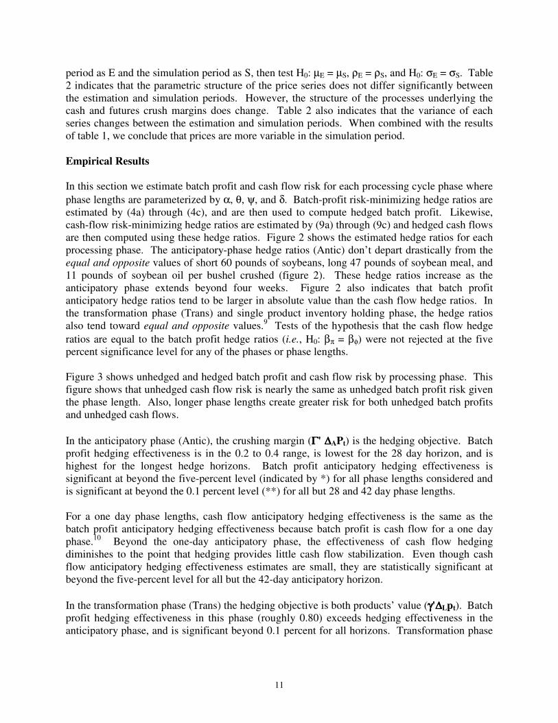
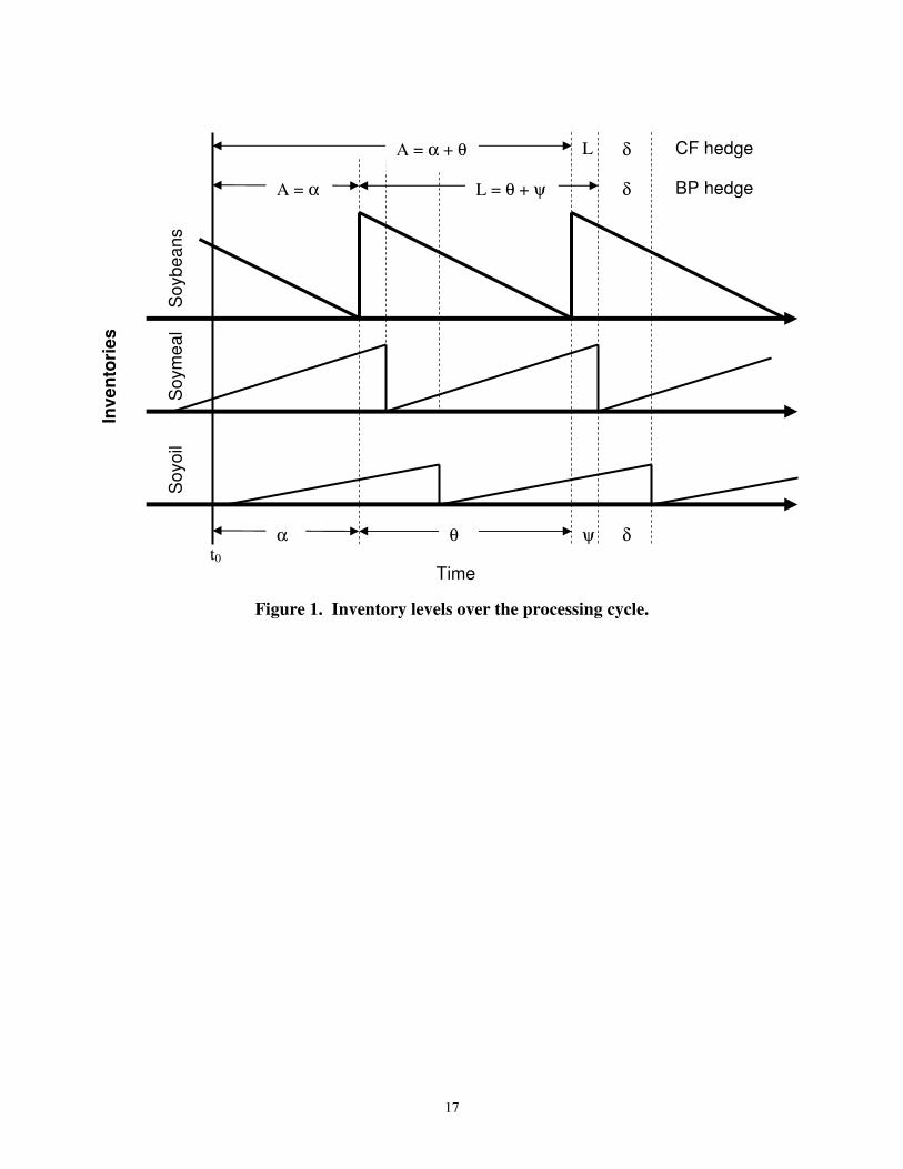
specify the delivery of a different commodity (i.e., a cross-hedge), or may specify non-commodity financial instruments (currencies, securities, indices, or weather). Other hedging strategies are defined in terms of the speculative soybean futures crush spread. In a one-to-one crush hedge, the processor is long one bushel in a soybean crush spread for each anticipated bushel to be processed. This strategy is identical to a one-to-one hedge if the soybean oil and the soybean meal are sold simultaneously. A generalization of the one-to-one crush hedge is the proportional crush hedge whereby the soybean processor employs a risk-minimizing crush spread that is proportional to the cash soybean market position. Various studies have examined these soybean-crush-hedging strategies. Tzang and Leuthold (1990) use weekly prices from January 1983 through June 1988 to investigate multi- and single-contract soybean processing hedges over 1 through 15-week hedging horizons. Fackler and McNew (1993) use monthly prices to examine three soybean processing hedging strategies: multi-contract hedges, single-contract hedges, and proportional crush-spread hedges. The multi-contract approach has recently been extended to cross hedging in the cottonseed-processing sector (Dahlgran 2000; Rahman, Turner, and Costa 2001). Some production hedges resemble processing hedges. These include the cattle feeding hedge using corn, feeder cattle, and live cattle futures (Leuthold and Mokler 1979; Shafer, Griffin and Johnson 1978), and the hog feeding hedge using live hog, soybean meal and corn futures (Kenyon and Clay 1987). The hedging methods in the studies mentioned thus far are of the Johnson, Anderson and Danthine type with the objective being the minimization of the variance of batch profits. Dahlgran (2005) demonstrated that when continuous processing is approximated with multiple batches, and when the traditional hedging approach is applied to each batch, annual aggregate profits are stabilized and each batch's profits are stabilized, but cash flow becomes more variable. With the exception of a study on cattle feeding done by Purcell and Rife, and Dahlgran's (2005) study of transaction frequency as a risk management strategy, cash flow hedging is largely unexplored and cash flow hedging strategies for commodity processors have yet to receive any attention. Empirical Model In this section we compare cash flow hedging with batch profit hedging and derive a cash flow risk minimizing hedge ratio estimator which provides managers with a tool to manage another type of price risk. Our model represents a process in which soybeans (60 pounds per bushel) are purchased periodically and then transformed into soybean meal (47 pounds per bushel of soybeans) and soybean oil (47 pounds per bushel of soybeans). As soybeans are processed, soybean inventories decline and product inventories accumulate. Figure 1 represents these relationships. Inventory cycles are of length θ and repeat n times during the year as annual throughput of y is processed. If t0 represents the current time, then α designates an anticipatory phase during which the coming processing cycle is planned Product sales are not assumed to occur concurrently nor are they assumed to occur concurrently with soybean purchases. Figure 1 indicates that soybean meal is sold first in the processing cycle but we more generally designate soybean products as 1 and 2 with the sale of product 1

6

occurring either before or concurrently with the sale of product 2. ψ designates the delay in the sale of product 1 after the exhaustion of input inventories, and δ designates the delay in the sale of product 2 after the sale of product 1. If ψ = δ = 0, then the input and output inventory cycle phases match as products are sold concurrently with the purchase of soybeans for the next cycle. This condition minimizes daily cash flow variability. The applicable prices are ps,t, the per bushel price paid for soybeans purchased at time t, and p1,t and p2,t the respective prices received for products 1 and 2 sold at time t. These prices are consolidated in the column vector Pt = [ ps,t , p1,t , p2,t ]' = [ ps,t : pt ]'. The production coefficients are contained in the 3 x 1 vector ΓΓΓΓ and are arranged to correspond to the price vector. Thus, ΓΓΓΓ = [ -1 , γ1 , γ2 ]' where γ1 and γ2 represent per bushel yields of products 1 and 2. The production coefficients are also represented by the 2 x 1 vector γγγγ = [ γ1 , γ2 ]' so ΓΓΓΓ' = [ -1 : γγγγ' ]. Without hedging, profits anticipated at time t, generated by the batch that will be initiated at the end of the anticipatory phase α are represented by u

tπ where

, 1 1, 2 2,( / ) [ ]ut s t t ty n p p p+α +α+θ+ψ +α+θ+ψ+δπ = − + γ + γ . (1a)

Expressing the yet to be determined prices as current prices plus changes over the processing phase gives

, , 1 1, 1, 1,

2 2, 2, 2, 2,

( / ) [ ( ) ( )

( )]

ut s t s t t t t

t t t t

y n p p p p p

p p p pα +α α +α θ+ψ +α+θ+ψ

α +α θ+ψ +α+θ+ψ δ +α+θ+ψ+δ

π = − + ∆ + γ + ∆ + ∆ +

γ + ∆ + ∆ + ∆ (1b)

where ∆dXt = Xt - Xt-d. This expression indicates that the profit outcome depends on the current crushing margin (-ps,t + γ1 p1,t + γ2 p2,t), the change in the crushing margin over the anticipatory period (-∆αps,t+α + γ1 ∆αp1,t+α + γ2 ∆αp2,t+α), the change in product prices after the soybeans are purchased but before the products are sold ( 1 1, 2 2,t tp pθ+ψ +α+θ+ψ θ+ψ +α+θ+ψγ ∆ + γ ∆ ), and the change in

the price of product 2 during the period when only it is held in inventory ( 2 2,tpδ +α+θ+ψ+δγ ∆ ). Price risk arises from these last three components. Equation (1b) can be expressed more succinctly as 2 2,( / ) [ ]u

t t t t ty n pα +α θ+ψ +α+θ+ψ δ +α+θ+ψ+δπ = + γ ∆P' P' + p' + . (1c) With hedging, profit becomes f, f,+ f,

h ut t t t tα +α θ+ψ +α+θ+ψ δ +α+θ+ψ+δπ = π + x' F + x' F + x' F (1d)

where xf,a represents futures positions held during phase a and F represents a vector of prices of the futures contracts used for hedging. This formulation designates futures positions during the anticipatory phase (xf,α), during the phase when both products are either implicitly stored in the input (θ) or explicitly stored as outputs (ψ) ( f,+x ), and during the phase when a single product

is stored ( f,x ). Futures positions differ in each phase because the price risks differ. In the

anticipatory phase (α) price risk is in the form of crush-margin change, in the transformation phase (θ+ψ) price risk is in the form of a change in either output price, and in the single-product holding phase (δ) price risk is in the form of a change in the single output price.

7

Suppose the firm's hedging objective is to minimize the variance of profit where

2

f, f, f,+ f,+ f, f,

f, f,+ f, 2

( | ) ( | ) ' '

2 ( / )

h ut t t tV V

y n

α α θ+ψ θ+ψ δ δ

α α θ+ψ θ+ψ δ δ

π Ω = π Ω + + +

+ + + F, F F, F F, F

F, P F, P F, p

x x x x x' x

(x' x' x' ) (2)

and ΣΣΣΣx,y represents the matrix of covariances between the variables in vectors x and y and Ωt represents the current information set. Minimizing this variance with respect to xf,α, xf,θ+ψ, and xf,δ gives the variance-minimizing futures positions for each of the periods α, θ+ψ, and δ. f, ( / ) y n

α α α α

−= −* 1 F, F F, Px ( ) (3a)

f,+ ( / ) y nθ+ψ θ+ψ θ+ψ θ+ψ

−= −* 1 F, F F, Px ( ) (3b)

2f, 2( / ) y n −= − γ

* 1 F, F F, px ( ) (3c)

Hedge ratios per bushel of soybeans processed for the phases α, θ+ψ and δ in figure 1 are estimated by the coefficients in the regression models1 ΓΓΓΓ' ∆∆∆∆αPt = ∆∆∆∆αF'α,t ββββα +εα,t, (4a) γγγγ' ∆∆∆∆θ+ψpt = ∆∆∆∆θ+ψF'θ+ψ,t ββββθ+ψ +εθ+ψ,t, and (4b) γ2∆δp2,t = ∆∆∆∆δF'δ,t ββββδ +εδ,t. (4c) The dependent variables respectively represent the change in the crush margin during the anticipatory phase (ΓΓΓΓ'∆∆∆∆αPt), the change in the value of both products during the period between the soybean purchase and the sale of the first product, (γγγγ'∆∆∆∆θ+ψpt), and the change in the value of the final product over the phase that it is held (γ2 ∆δp2,t). This approach exemplifies current for soybean processing hedging methods. We now examine anticipated cash flow and methods for hedging it.2 Without hedging, cash flow currently anticipated for the final-product sales period (figure 1) is3 , 1 1, 1 1,( / )[ ]u

t s t t ty n p p p+α+θ +α+θ+ψ +α+θ+ψφ = − + γ + γ . (5a) Rearranging to isolate the current given prices from unknown future spot prices gives 2 2,( / ) [ ]u

t t t t ty n pα+θ +α+θ ψ +α+θ+ψ δ +α+θ+ψ+δφ = + + + γ ∆P' P' p' . (5b)

This expression differs from (1c) in that over the processing phase (θ) the crushing margin (P' ) is at risk rather than the value of both products (p' ).4 This difference reflects the notion that the embodiment of products in specific soybean purchases is immaterial from the standpoint of cash flow. With hedging, cash flows result from both spot market transactions as well as the daily revaluation of futures positions. By exchange regulations (Chicago Board of Trade, 2006), initial and maintenance hedging margins in the soybean complex are identical so that every daily futures price change requires margin account resettlement. Thus, cash flows are expressed as f, f, f,1 1 1

'h ut t t t t

α+θ ψ δα+θ +τ +α+θ+τ +α+θ+ψ+ττ= τ= τ=

φ = φ + + + x F x' F x' F (5c)

where ∆F represents the day to day futures-price change. This expression differs from (1d) in that it recognizes cash flows from futures positions on each day that the position is held whereas (1d) recognizes only the aggregate cash flow of the position at its termination.5 The other difference between (5c) and (1d) is that the processing phase (θ) appears in the anticipatory period rather than in the two-product inventory period. The variance of cash flow over the transaction cycle

8

f,+ f,+ f, f, f, f,1 1 1

' 'f,+ f,1 1

f,

( | ) ( | ) '

2( / )

h ut t t t

t t t t

t

V V

y n

α+θ ψ δψ ψτ= τ= τ=

α+θ ψ+τ α+θ +α+θ ψ +α+θ+τ ψ +α+θ+ψτ= τ=

+α+θ+ψ+

φ Ω = φ Ω + + + +

+ +

+

F,F F,F F,Fx x x' x x' x

x' Cov(F , P' ) x' Cov(F , p )

x' Cov(F ,1b t bp

δτ δ +α+θ+ψ+δτ=

γ , )

(6)

explicitly recognizes the daily cash flows attributed to futures position resettlement. Minimizing the variance with respect to the futures positions for each of the three periods gives f,+ 1

( ) ( / ) ( ) 0t ty n Covα+θ

+τ α+θ +α+θτ=α + θ + =F,F x F' P (7a)

f, 1 ( / ) ( ) 0t ty n Cov

ψ+α+θ+τ ψ +α+θ+ψτ=

ψ + =F,F x F' p (7b)

f, 2 21 ( / ) ( ) 0t ,t A y n Cov p

δ+α+θ+ψ+τ δ + +ψ+τ=

δ + ∆ γ =F,F x F' (7c)

where f,+ f, f,, , and x x x indicate the cash flow risk minimizing futures positions during the three

periods represented by the phases α+θ, ψ and δ. The covariances in (7a) through (7c) can be further simplified. For example, in (7a)6

1( ) [ ' ]t t t tCov Cov

α+θ+τ α+θ +α+θ α+θ +α+θ α+θ +α+θτ=

= F' P F P (8)

Thus, the cash flow risk minimizing futures positions for the phases of the processing cycle are x

tt P,FFF,f, θ+α+θ+αθ+α+θ+α

−θ+α θ+α−= 1] )( [ )/(~ ny (9a)

1f, ( / )( )

t ty n

ψ +α+θ+ψ ψ +α+θ+ψ

−= − ψF,F F px (9b)

,

1( / )( )t b tp by n+α+θ+ψ+δ +α+θ+ψ+δ

−= − δ γ f, F,F F

x (9c)

These expressions are similar to (3a) through (3c), respectively, except that the futures-price-change covariance matrix (ΣΣΣΣ∆∆∆∆F,∆∆∆∆F) represents day-to-day changes rather than changes over the hedging interval. The hedge ratios in (9a) through (9c) can be estimated from moment matrices. However, for the sake of comparison, we seek to determine how to use regression analysis to estimate these hedge ratios. Because of the equations’ similarity, we focus on (9a) knowing that the analysis of (9b) and (9c) will proceed similarly. To simplify, let A represent the length of the anticipatory period (=α+θ) and assume that A is one processing cycle (θ) so α=0. To incorporate standard regression notation, let X = ∆∆∆∆F where X is NA x k with N representing the number of processing cycles represented in the data set, and k the number of futures contracts considered as hedge vehicles. Let Z = ∆∆∆∆AF where Z is N x k and let Y = ∆∆∆∆AP where Y is N x 3.7 Then FF, = X'X /

NA, ˆA A F, P = Z'Y / N and

( )1

1f, +

1ˆ ( / ) ( / ) y n y nA NA N

−−

α θ = − = −

X'X Z'Yx X'X Z'Y . (10a)

But Z = ( IN ⊗ 1'A)∆∆∆∆F = ( IN ⊗ 1'A) X and Y = ( IN ⊗ 1'A) ∆∆∆∆P. Thus Z'Y = X' ( IN ⊗ 1' 1 ) ∆∆∆∆P so ( ) 1

f,+ˆ ( / ) x n

−= ⊗Nx X'X X'(I 1 1') P (10b) Thus, the cash flow risk minimizing hedge ratios are estimated by the regression model (IN ⊗ 1 1') ∆∆∆∆P ΓΓΓΓ = ∆∆∆∆F ββββα+θ + εεεε (11a) The explanatory variables in this formulation are daily futures price changes. The dependent variable is the change in the crushing margin, ∆∆∆∆P ΓΓΓΓ, summed over the hedging period,

9

(IN ⊗ 1') ∆∆∆∆P ΓΓΓΓ, with each daily observation in a hedging period being the sum of the daily changes over the entire hedging period, (IN ⊗⊗⊗⊗ 1)(IN ⊗⊗⊗⊗ 1') ∆∆∆∆P ΓΓΓΓ. We recognize that this formulation implies that cash flow risk reduction will be difficult to achieve through hedging. Data Considerations Data to empirically test the analytical model were obtained from BarChart.com. These data consist of daily observations of cash and futures prices for soybeans, soybean oil and soybean meal from January 1990 through December 2005. The cash prices apply to central Illinois. The futures prices are for all soybean, soybean oil, and soybean meal contracts traded on the Chicago Board of Trade during this time period. Soybean meal characteristics changed during the sample period as the deliverable grade specified by the futures contract changed from 44 percent to 48 percent protein beginning with the September 1992 contract. The cash price data were for 44 percent protein soybean meal through November 17, 1992 and for 48 percent protein thereafter. During a transition period from November 18, 1992 through December 26, 2001 the Wall Street Journal reported prices for both 44 percent and 48 percent protein soybean meal. The following procedure was used to convert 44 percent soybean meal prices to the new 48 percent standard. Cash prices for both 44 percent and 48 percent soybean meal were collected for each Wednesday during the period when both were quoted. The ordinary least squares relationship between the 44-percent and 48-percent meal prices was estimated as pM48,t = 5.96 + 1.0221 pM44,t Observations = 476, R2 = 0.997 (0.476) (0.00257) where pM48,t is the 48-percent soybean meal cash price in period t, pM44,t is the 44-percent soybean meal cash price in period t, and standard errors are in parentheses. This relationship was used to generate fitted values for 48-percent soybean meal cash prices prior to November 18, 1992 and to generate fitted values for 48-percent soybean meal futures prices for contracts that matured prior to September 1992. The fitted values were used as proxies for the unobservable 48-percent cash and futures prices. The high regression R2 assures that these fitted values are good proxies for the unobservable prices. The model assumes that the processing phase parameters (α, θ, ψ, and δ) can take any integer value but empirical analysis must accommodate the idiosyncrasies of the business calendar. To illustrate, suppose α = ψ = δ = 0. Our daily observations permit profit and cash flow computations for θ = 1. However, transformation cycles of two days through one week clash with the market's weekend closures making the cycle length ambiguous. For example, if θ is 3 calendar days, then prices will be unavailable on weekends, and if θ is set to three business days, then the observations become unevenly spaced in time because of weekends. We select values of α, θ, ψ, and δ that are consistent with daily, weekly, and multi-week cycles. Weekly and multi-week cycles will be assumed to start on Wednesdays. When a holiday falls on Wednesday, we use Tuesday's prices but assume that those prices were observed on Wednesday to preserve evenly-spaced observations.

10

To determine the effectiveness of cash flow hedging and to compare the effectiveness of cash flow hedging to batch profit hedging we assume a range of phase lengths that correspond to the hedge horizons studied by Tzang and Leuthold, and Fackler and McNew. For batch profit hedging, we will examine anticipatory phases (α) of 1, 7, 14, 28, 42, 56, and 91 days, temporal differences between input and output prices (θ+ψ) of 1, 7, 14, 28, 42, and 56 days, and product sales timing differences (δ) of 0, 1, 7, 14, and 28 days. For comparison, we will examine cash flow hedging effectiveness for anticipatory phases (α+θ) of 1, 7, 14, 28, 42, 56, and 91 days, input-purchase output-sales time lags (ψ) of 1, 7, 14, 28, 42, and 56 days, and product sales time differences (δ) of 1, 7, 14, and 28 days. The futures contracts used for hedging were selected according to the following rules. First, only contract maturities that permit the construction of a pure crush spread, where the soybean, soybean oil, and soybean meal contracts all have the same maturity, are used. This eliminates October and December soybean oil and meal contracts because soybean contracts are not traded for these months. Likewise, November soybeans are eliminated because November soybean oil and meal are not traded. This leaves the January, March, May, July, and September soybean, soybean oil and soybean meal contracts to be used in the hedging portfolio. Second, only contracts with at least seven days to maturity at the time of hedge closure were used. Subject to these two broad exclusions, hedges used the nearby futures contract maturity where the nearby maturity is defined by the time of the final cash market transaction. As an example, if a batch of soybean meal is sold two weeks after the soybean oil and if soybeans were purchased for the batch six weeks before the soybean oil is sold, then the nearby maturity for all three futures contracts is defined relative to the final soybean meal sale. This definition precludes the construction of crushing hedges with inter-temporal features. The 1990 through 2005 sample period was broken into a 1990 through 1999 estimation period and a 2000 through 2005 simulation period. The data that result from the application of the above rules are summarized in table 1. In anticipation of estimating the mean prior to estimating the variance, table 1 reports statistics for the model pt = µ(1-ρ) + ρ pt-1 +et for cash and futures prices and crushing margins for the entire sample period and each sub period.8 If ρ = 1, then the series follows a random walk so that the conditional variance should be computed as the sum of squared price changes. Alternatively, if ρ = 0, then the variance should be computed as deviations about the sample average. For intermediate and significant values of ρ, the variance should be computed as deviations about the fitted value given by the model. The Dickey-Fuller Φ1 statistics in table 1 test H0: b = 1 and a = 0 in the model pt = a + b pt-1 + et. This hypothesis is consistently rejected for the cash crush margin implying that the cash crush margin tends to wander back to an equilibrium level. Also reported in table 1 are the estimated serial correlation coefficients. All are close to 1, even those for which the random-walk hypothesis is rejected. The estimates of ρ indicate the while the crush margins wander back to equilibrium levels, they do so slowly. The estimated model will be used to simulate outcomes in the 2000 through 2005 simulation period. Poor simulation results could be caused by a change in the structure of the process that generates the data between the estimation and the simulation period. Table 2 reports test results for differences between the estimation and the simulation periods. We designate the estimation

11

period as E and the simulation period as S, then test H0: µE = µS, ρE = ρS, and H0: σE = σS. Table 2 indicates that the parametric structure of the price series does not differ significantly between the estimation and simulation periods. However, the structure of the processes underlying the cash and futures crush margins does change. Table 2 also indicates that the variance of each series changes between the estimation and simulation periods. When combined with the results of table 1, we conclude that prices are more variable in the simulation period.

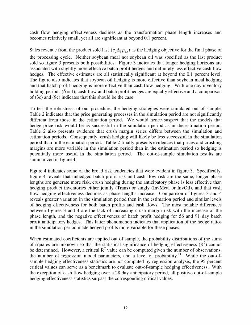
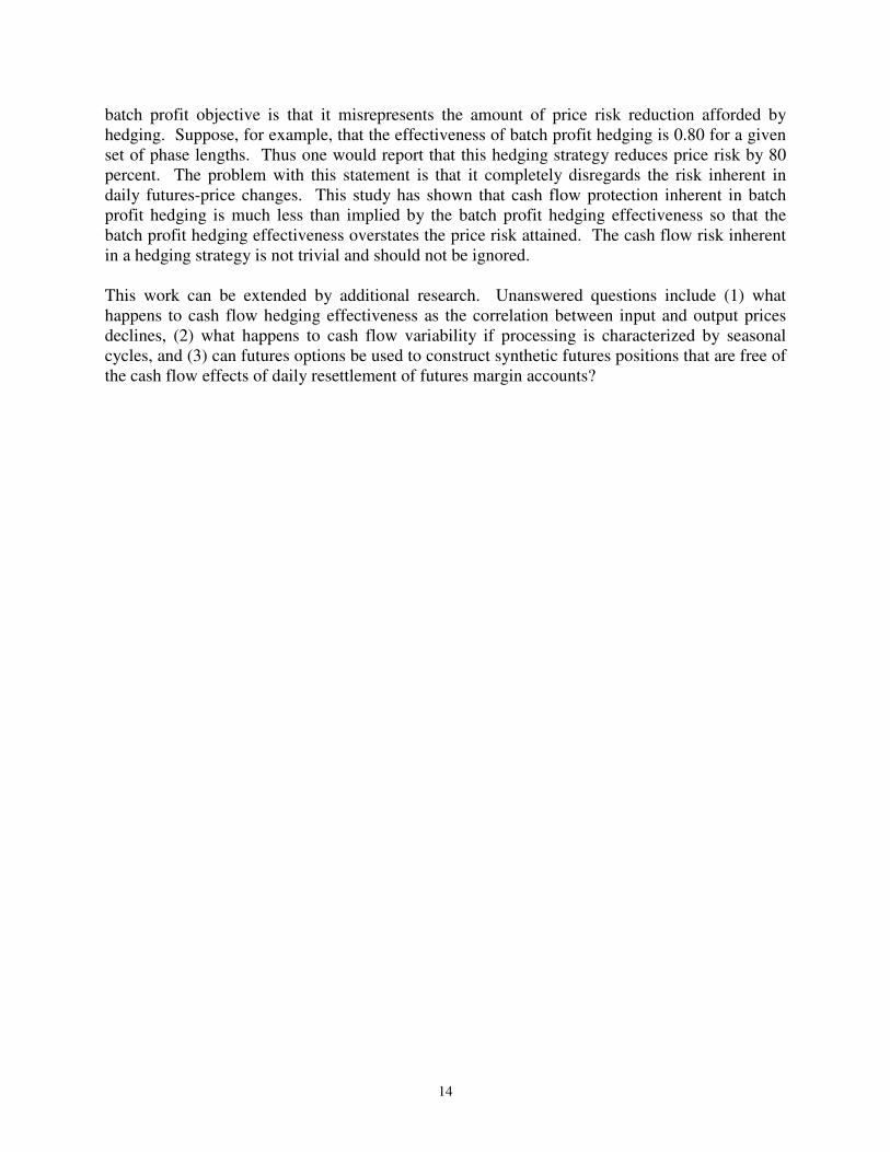
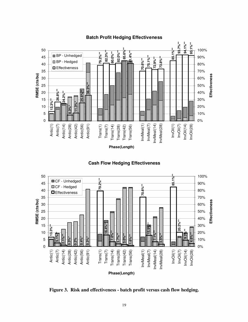
Empirical Results In this section we estimate batch profit and cash flow risk for each processing cycle phase where phase lengths are parameterized by α, θ, ψ, and δ. Batch-profit risk-minimizing hedge ratios are estimated by (4a) through (4c), and are then used to compute hedged batch profit. Likewise, cash-flow risk-minimizing hedge ratios are estimated by (9a) through (9c) and hedged cash flows are then computed using these hedge ratios. Figure 2 shows the estimated hedge ratios for each processing phase. The anticipatory-phase hedge ratios (Antic) don’t depart drastically from the equal and opposite values of short 60 pounds of soybeans, long 47 pounds of soybean meal, and 11 pounds of soybean oil per bushel crushed (figure 2). These hedge ratios increase as the anticipatory phase extends beyond four weeks. Figure 2 also indicates that batch profit anticipatory hedge ratios tend to be larger in absolute value than the cash flow hedge ratios. In the transformation phase (Trans) and single product inventory holding phase, the hedge ratios also tend toward equal and opposite values.9 Tests of the hypothesis that the cash flow hedge ratios are equal to the batch profit hedge ratios (i.e., H0: βπ = βφ) were not rejected at the five percent significance level for any of the phases or phase lengths. Figure 3 shows unhedged and hedged batch profit and cash flow risk by processing phase. This figure shows that unhedged cash flow risk is nearly the same as unhedged batch profit risk given the phase length. Also, longer phase lengths create greater risk for both unhedged batch profits and unhedged cash flows. In the anticipatory phase (Antic), the crushing margin (ΓΓΓΓ' ∆∆∆∆APt) is the hedging objective. Batch profit hedging effectiveness is in the 0.2 to 0.4 range, is lowest for the 28 day horizon, and is highest for the longest hedge horizons. Batch profit anticipatory hedging effectiveness is significant at beyond the five-percent level (indicated by *) for all phase lengths considered and is significant at beyond the 0.1 percent level (**) for all but 28 and 42 day phase lengths. For a one day phase lengths, cash flow anticipatory hedging effectiveness is the same as the batch profit anticipatory hedging effectiveness because batch profit is cash flow for a one day phase.10 Beyond the one-day anticipatory phase, the effectiveness of cash flow hedging diminishes to the point that hedging provides little cash flow stabilization. Even though cash flow anticipatory hedging effectiveness estimates are small, they are statistically significant at beyond the five-percent level for all but the 42-day anticipatory horizon. In the transformation phase (Trans) the hedging objective is both products’ value (γγγγ'∆∆∆∆Lpt). Batch profit hedging effectiveness in this phase (roughly 0.80) exceeds hedging effectiveness in the anticipatory phase, and is significant beyond 0.1 percent for all horizons. Transformation phase

12

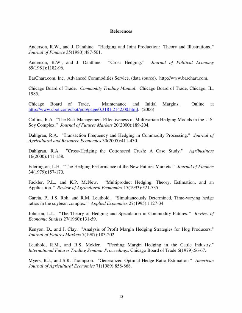
cash flow hedging effectiveness declines as the transformation phase length increases and becomes relatively small, yet all are significant at beyond 0.1 percent. Sales revenue from the product sold last 2 2,( )tpδγ ∆ is the hedging objective for the final phase of the processing cycle. Neither soybean meal nor soybean oil was specified as the last product sold so figure 3 presents both possibilities. Figure 3 indicates that longer hedging horizons are associated with slightly more effective batch profit hedges and definitely less effective cash flow hedges. The effective estimates are all statistically significant at beyond the 0.1 percent level. The figure also indicates that soybean oil hedging is more effective than soybean meal hedging and that batch profit hedging is more effective than cash flow hedging. With one day inventory holding periods (δ = 1), cash flow and batch profit hedges are equally effective and a comparison of (3c) and (9c) indicates that this should be the case. To test the robustness of our procedure, the hedging strategies were simulated out of sample. Table 2 indicates that the price generating processes in the simulation period are not significantly different from those in the estimation period. We would hence suspect that the models that hedge price risk would be as successful in the simulation period as in the estimation period. Table 2 also presents evidence that crush margin series differs between the simulation and estimation periods. Consequently, crush hedging will likely be less successful in the simulation period than in the estimation period. Table 2 finally presents evidences that prices and crushing margins are more variable in the simulation period than in the estimation period so hedging is potentially more useful in the simulation period. The out-of-sample simulation results are summarized in figure 4. Figure 4 indicates some of the broad risk tendencies that were evident in figure 3. Specifically, figure 4 reveals that unhedged batch profit risk and cash flow risk are the same, longer phase lengths are generate more risk, crush hedging during the anticipatory phase is less effective than hedging product inventories either jointly (Trans) or singly (InvMeal or InvOil), and that cash flow hedging effectiveness declines as phase lengths increase. Comparison of figures 3 and 4 reveals greater variation in the simulation period then in the estimation period and similar levels of hedging effectiveness for both batch profits and cash flows. The most notable differences between figures 3 and 4 are the lack of increasing crush margin risk with the increase of the phase length, and the negative effectiveness of batch profit hedging for 56 and 91 day batch profit anticipatory hedges. This latter phenomenon indicates that application of the hedge ratios in the simulation period made hedged profits more variable for these phases. When estimated coefficients are applied out of sample, the probability distributions of the sums of squares are unknown so that the statistical significance of hedging effectiveness (R2) cannot be determined. However, a critical R2 value can be computed given the number of observations, the number of regression model parameters, and a level of probability.11 While the out-of-sample hedging effectiveness statistics are not computed by regression analysis, the 95 percent critical values can serve as a benchmark to evaluate out-of-sample hedging effectiveness. With the exception of cash flow hedging over a 28 day anticipatory period, all positive out-of-sample hedging effectiveness statistics surpass the corresponding critical values.

13

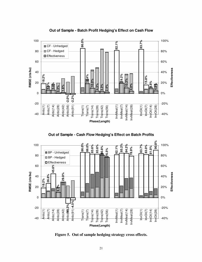
For our final simulation, we examine how batch profit hedging affects cash flow risk and how cash flow hedging affects batch profit risk. These simulations are summarized in figure 5 and generally reflect the finding that the cash flow hedge ratios are not significantly different from batch profit hedge ratios. The upper panel of figure 5 shows the simulated impact on cash flow variability of hedging batch profit. As in the previous cases, longer hedge horizons are associated with less risk reduction. The lower panel of figure 5 shows the simulated impact of cash flow hedging on batch profits. A comparison of the lower panel of figure 5 with the upper panel of figure 4 shows that the application of the cash flow risk minimizing hedge ratios has the desirable effects of effectively hedging inventories (Teans, InvMeal and InvOil) regardless of the hedge horizon, and is less destabilizing of the crush margin (Antic) than is the batch profit hedge ratios. Summary and Conclusions The objectives of this study were to determine how to hedge cash flows from commodity processing, to compare the analytical solution for cash flow hedging to the traditional batch profit hedging solution, and to empirically estimate the effectiveness of cash flow hedging. In accomplishing these objectives, we first developed the empirical method for determining cash flow variability and for estimating cash-flow-risk-minimizing hedge ratios. The analytical solution for computing these ratios is similar to the method for computing traditional batch profit-risk-minimizing hedge ratios. The primary difference is that cash-flow-risk-minimizing hedge ratios balance the risk of cash flow destabilizing spot price changes against the cash flow destabilizing effects of daily futures price changes. A multiple regression estimator of cash-flow risk minimizing hedge ratios was derived. In the empirical analysis we found that cash flow risk minimizing hedge ratios are not significantly different from batch profit risk minimizing hedge ratios, that risk increases with the processing phase length, that less risk is associated with crush margin than with product inventory holding, that hedging crush margin risk is less effective than hedging product inventories, that cash flow hedging is less effective than batch profit hedging, that the effectiveness of cash flow hedging declines as the phase length increases, and that cash flow hedging effectiveness is significant, even though it may be small. Furthermore, our empirical model suggested that the timing of hedging strategies differs between cash flow hedging and batch profit hedging. Specifically, given the processing cycle, the crush hedge duration is α under batch profit hedging and α+θ under cash flow hedging. In addition, the time for hedging the products’ value is θ+ψ under batch profit hedging and ψ under cash flow hedging. Finally, the single product inventory hedge is δ for both hedge targets. As a result, cash flow hedging will be less effective than batch profit hedging for two reasons. First the cash flow hedging strategy spends more time (θ) in a crush hedge at the expense of the inventory hedge and the crush hedge is less effective than the inventory hedge given the phase length. Also, cash flow hedging explicitly recognizes the day-to-day impacts of futures prices changes that are disregarded under batch profit hedging. In conclusion, batch profit hedging is more effective than cash flow hedging. Is this reason enough for batch profits to be the dominant hedging objective? One danger in focusing on the

14

batch profit objective is that it misrepresents the amount of price risk reduction afforded by hedging. Suppose, for example, that the effectiveness of batch profit hedging is 0.80 for a given set of phase lengths. Thus one would report that this hedging strategy reduces price risk by 80 percent. The problem with this statement is that it completely disregards the risk inherent in daily futures-price changes. This study has shown that cash flow protection inherent in batch profit hedging is much less than implied by the batch profit hedging effectiveness so that the batch profit hedging effectiveness overstates the price risk attained. The cash flow risk inherent in a hedging strategy is not trivial and should not be ignored. This work can be extended by additional research. Unanswered questions include (1) what happens to cash flow hedging effectiveness as the correlation between input and output prices declines, (2) what happens to cash flow variability if processing is characterized by seasonal cycles, and (3) can futures options be used to construct synthetic futures positions that are free of the cash flow effects of daily resettlement of futures margin accounts?

15

References

Anderson, R.W., and J. Danthine. “Hedging and Joint Production: Theory and Illustrations.” Journal of Finance 35(1980):487-501.

Anderson, R.W., and J. Danthine. “Cross Hedging.” Journal of Political Economy 89(1981):1182-96.

BarChart.com, Inc. Advanced Commodities Service. (data source). http://www.barchart.com.

Chicago Board of Trade. Commodity Trading Manual. Chicago Board of Trade, Chicago, IL, 1985.

Chicago Board of Trade, Maintenance and Initial Margins. Online at http://www.cbot.com/cbot/pub/page/0,3181,2142,00.html. (2006)

Collins, R.A. “The Risk Management Effectiveness of Multivariate Hedging Models in the U.S. Soy Complex.” Journal of Futures Markets 20(2000):189-204.

Dahlgran, R.A. "Transaction Frequency and Hedging in Commodity Processing." Journal of Agricultural and Resource Economics 30(2005):411-430.

Dahlgran, R.A. "Cross-Hedging the Cottonseed Crush: A Case Study." Agribusiness 16(2000):141-158.

Ederington, L.H. “The Hedging Performance of the New Futures Markets.” Journal of Finance 34(1979):157-170.

Fackler, P.L., and K.P. McNew. “Multiproduct Hedging: Theory, Estimation, and an Application.” Review of Agricultural Economics 15(1993):521-535.

Garcia, P., J.S. Roh, and R.M. Leuthold. “Simultaneously Determined, Time-varying hedge ratios in the soybean complex.” Applied Economics 27(1995):1127-34.

Johnson, L.L. “The Theory of Hedging and Speculation in Commodity Futures.” Review of Economic Studies 27(1960):131-59.

Kenyon, D., and J. Clay. "Analysis of Profit Margin Hedging Strategies for Hog Producers." Journal of Futures Markets 7(1987):183-202.

Leuthold, R.M., and R.S. Mokler. "Feeding Margin Hedging in the Cattle Industry." International Futures Trading Seminar Proceedings, Chicago Board of Trade 6(1979):56-67.

Myers, R.J., and S.R. Thompson. "Generalized Optimal Hedge Ratio Estimation." American Journal of Agricultural Economics 71(1989):858-868.

16

Purcell, Wayne D., and Don A. Riffe. "The Impact of Selected Hedging Strategies on the Cash Flow Position of Cattle Feeders." Southern Journal of Agricultural Economics, 12(July 1980) 85-93.

Rahman, S.M., S.C. Turner, and E.F. Costa. "Cross-Hedging Cottonseed Meal." Journal of Agribusiness 19(2001):163-171.

Stein, J.J. "The Simultaneous Determination of Spot and Futures Prices." American Economic Review 51(1961):1012-1025.

Shafer, C.E., W.L Griffin, and L.D. Johnson "Integrated Cattle Feeding Hedging Strategies, 1972-1976." Southern Journal of Agricultural Economics 10(1978):35-42.

Tzang, D., and R.M. Leuthold. “Hedge Ratios under Inherent Risk Reduction in a Commodity Complex.” Journal of Futures Markets 10(1990):497-504.

17

Figure 1. Inventory levels over the processing cycle.

A = α L = θ + ψ

ψ δ θ

Soy

bean

s

α

δ BP hedge

CF hedge A = α + θ δ L

Soy

mea

l S

oyoi

l

Time

Inve

ntor

ies

t0

18

Estimated Hedge Ratios

-100

-80

-60

-40

-20

0

20

40

60

80

100A

ntic

(1)

Ant

ic(7

)

Ant

ic(1

4)

Ant

ic(2

8)

Ant

ic(4

2)

Ant

ic(5

6)

Ant

ic(9

1)

Tra

ns(1

)

Tra

ns(7

)

Tra

ns(1

4)

Tra

ns(2

8)

Tra

ns(4

2)

Mea

l Inv

(1)

Mea

l Inv

(7)

Mea

l Inv

(14)

Mea

l Inv

(28)

Oil

Inv(

1)

Oil

Inv(

7)

Oil

Inv(

14)

Oil

Inv(

28)

Processing Phase (Length)

lbs

futu

res/

bu

soyb

eans

BP - Soy MealBP - Soy OilBP - SoybeansCF - Soy MealCF - Soy OilCF - Soybeans

Figure 2. Estimated hedge ratios by phase and phase length.

19

Batch Profit Hedging Effectiveness

13.3

%** 26

.8%

**

24.2

%**

8.3%

*

11.3

%* 25

.6%

** 36.3

%**

79.2

%**

82.3

%**

80.0

%**

82.0

%**

85.6

%**

81.4

%**

70.6

%**

75.1

%**

72.9

%**

73.8

%** 85

.1%

**

93.7

%**

94.1

%**

93.1

%**

0

5

10

15

20

25

30

35

40

45

50A

ntic

(1)

Ant

ic(7

)

Ant

ic(1

4)

Ant

ic(2

8)

Ant

ic(4

2)

Ant

ic(5

6)

Ant

ic(9

1)

Tran

s(1)

Tran

s(7)

Tran

s(14

)

Tran

s(28

)

Tran

s(42

)

Tran

s(56

)

InvM

eal(1

)

InvM

eal(7

)

InvM

eal(1

4)

InvM

eal(2

8)

InvO

il(1)

InvO

il(7)

InvO

il(14

)

InvO

il(28

)

Phase(Length)

RM

SE

(cts

/bu)

0%

10%

20%

30%

40%

50%

60%

70%

80%

90%

100%

Eff

ectiv

enes

s

BP - Unhedged

BP - Hedged

Effectiveness

Cash Flow Hedging Effectiveness

0.2%

13.3

%**

5.1%

**

2.1%

**

0.3%

*

0.4%

*

0.3%

*

79.2

%**

16.4

%**

7.0%

**

3.7%

**

3.0%

**

1.6%

**

70.6

%**

15.9

%**

7.1%

**

3.5%

**

85.1

%**

20.2

%**

9.2%

**

4.6%

**

0

5

10

15

20

25

30

35

40

45

50

Ant

ic(1

)

Ant

ic(7

)

Ant

ic(1

4)

Ant

ic(2

8)

Ant

ic(4

2)

Ant

ic(5

6)

Ant

ic(9

1)

Tra

ns(1

)

Tra

ns(7

)

Tran

s(14

)

Tran

s(28

)

Tran

s(42

)

Tran

s(56

)

InvM

eal(1

)

InvM

eal(7

)

InvM

eal(1

4)

InvM

eal(2

8)

InvO

il(1)

InvO

il(7)

InvO

il(14

)

InvO

il(28

)

Phase(Length)

RM

SE

(cts

/bu)

0%

10%

20%

30%

40%

50%

60%

70%

80%

90%

100%

Eff

ectiv

enes

s

CF - UnhedgedCF - HedgedEffectiveness

Figure 3. Risk and effectiveness - batch profit versus cash flow hedging.

20

Out of Sample Batch Profit Hedging Effectiveness

18.2

% 26.2

%

48.2

%

12.8

%

42.7

%

-33.

7%

-39.

7%

86.0

%

86.0

%

87.5

%

85.2

%

80.8

%

85.8

%

82.1

%

84.8

%

86.2

%

79.3

%

83.7

%

85.4

%

88.8

%

94.1

%

-40

-20

0

20

40

60

80

100A

ntic

(1)

Ant

ic(7

)

Ant

ic(1

4)

Ant

ic(2

8)

Ant

ic(4

2)

Ant

ic(5

6)

Ant

ic(9

1)

Tran

s(1)

Tran

s(7)

Tran

s(14

)

Tran

s(28

)

Tran

s(42

)

Tran

s(56

)

InvM

eal(1

)

InvM

eal(7

)

InvM

eal(1

4)

InvM

eal(2

8)

InvO

il(1)

InvO

il(7)

InvO

il(14

)

InvO

il(28

)

Phase(Length)

RM

SE

(cts

/bu)

-40%

-20%

0%

20%

40%

60%

80%

100%

Eff

ectiv

enes

s

BP - Unhedged

BP - Hedged

Effectiveness

Out of Sample Cash Flow Hedging Effectiveness

18.2

%

6.0%

5.5%

0.3%

1.1%

-0.7

%

-0.5

%

86.0

%

18.6

%

9.5%

4.2%

3.3%

2.0%

82.1

%

19.8

%

10.2

%

4.0%

83.7

%

15.3

%

8.1%

4.7%

-40

-20

0

20

40

60

80

100

Ant

ic(1

)

Ant

ic(7

)

Ant

ic(1

4)

Ant

ic(2

8)

Ant

ic(4

2)

Ant

ic(5

6)

Ant

ic(9

1)

Tran

s(1)

Tran

s(7)

Tran

s(14

)

Tran

s(28

)

Tran

s(42

)

Tran

s(56

)

InvM

eal(1

)

InvM

eal(7

)

InvM

eal(1

4)

InvM

eal(2

8)

InvO

il(1)

InvO

il(7)

InvO

il(14

)

InvO

il(28

)

Phase(Length)

RM

SE

(cts

/bu)

-40%

-20%

0%

20%

40%

60%

80%

100%

Eff

ectiv

enes

s

CF - Unhedged

CF - Hedged

Effectiveness

Figure 4. Out of sample hedging effeciveness.

21

Out of Sample - Batch Profit Hedging's Effect on Cash Flow

18.2

%

5.8%

5.8%

0.3% 1.6%

-2.0

%

-2.2

%

86.0

%

18.4

%

10.0

%

4.3%

3.3%

2.4%

82.1

%

19.2

%

10.3

%

4.0%

83.7

%

15.8

%

8.8%

4.8%

-40

-20

0

20

40

60

80

100A

ntic

(1)

Ant

ic(7

)

Ant

ic(1

4)

Ant

ic(2

8)

Ant

ic(4

2)

Ant

ic(5

6)

Ant

ic(9

1)

Tran

s(1)

Tran

s(7)

Tran

s(14

)

Tran

s(28

)

Tran

s(42

)

Tran

s(56

)

InvM

eal(1

)

InvM

eal(7

)

InvM

eal(1

4)

InvM

eal(2

8)

InvO

il(1)

InvO

il(7)

InvO

il(14

)

InvO

il(28

)

Phase(Length)

RM

SE

(cts

/bu)

-40%

-20%

0%

20%

40%

60%

80%

100%

Eff

ectiv

enes

s

CF - Unhedged

CF - Hedged

Effectiveness

Out of Sample - Cash Flow Hedging's Effect on Batch Profits

18.2

% 26.8

%

45.6

%

9.7%

29.8

%

-11.

3% -4.5

%

86.0

%

86.0

%

83.6

%

83.6

%

80.8

%

76.5

%

82.1

%

85.2

%

84.2

%

78.9

%

83.7

%

83.0

%

81.0

% 90.8

%

-40

-20

0

20

40

60

80

100

Ant

ic(1

)

Ant

ic(7

)

Ant

ic(1

4)

Ant

ic(2

8)

Ant

ic(4

2)

Ant

ic(5

6)

Ant

ic(9

1)

Tran

s(1)

Tran

s(7)

Tran

s(14

)

Tran

s(28

)

Tran

s(42

)

Tran

s(56

)

InvM

eal(1

)

InvM

eal(7

)

InvM

eal(1

4)

InvM

eal(2

8)

InvO

il(1)

InvO

il(7)

InvO

il(14

)

InvO

il(28

)

Phase(Length)

RM

SE

(cts

/bu)

-40%

-20%

0%

20%

40%

60%

80%

100%

Eff

ectiv

enes

s

BP - Unhedged

BP - Hedged

Effectiveness

Figure 5. Out of sample hedging strategy cross effects.

22

Table 1. Sample data descriptive statistics.

Dickey Fuller test statisticsa Price series Units N Avg StdDev Φ1

b ρ RMSE

Estimation and simulation period (1990-2005) Cash prices Soybeans ¢/bu 4026 593.06 112.99 3.25 0.9967 8.62 Soybean oil ¢/lb 4026 22.08 4.66 2.65 0.9975 0.296 Soybean meal $/cwt 4026 190.93 38.78 3.93 0.9964 2.96 Crush margin ¢/bu 4026 98.47 26.66 33.91** 0.9692 5.85 Futures prices Soybeans ¢/bu 4031 604.81 110.04 0.56 0.9988 7.71 Soybean oil ¢/lb 4031 22.11 4.09 1.93 0.9977 0.277 Soybean meal $/cwt 4031 188.23 36.14 0.38 0.9998 2.58 Crush margin ¢/bu 4031 80.69 20.40 3.10 0.9952 2.46 Estimation period (1990-1999) Cash prices Soybeans ¢/bu 2526 608.98 93.79 0.61 0.9982 7.1 Soybean oil ¢/lb 2526 23.03 3.55 0.88 0.9978 0.28 Soybean meal $/cwt 2526 191.94 39.10 1.38 0.9976 2.71 Crush margin ¢/bu 2526 95.36 28.59 11.88** 0.9820 4.92 Futures prices Soybeans ¢/bu 2524 620.57 91.18 0.03 0.9997 6.86 Soybean oil ¢/lb 2524 23.11 3.28 0.68 0.9981 0.259 Soybean meal $/cwt 2524 189.84 35.01 0.99 1.0018 2.25 Crush margin ¢/bu 2524 79.71 22.38 0.00 1.0000 2.25 Simulation period (2000-2005) Cash prices Soybeans ¢/bu 1500 566.26 135.34 2.35 0.9952 10.71 Soybean oil ¢/lb 1500 20.48 5.75 1.69 0.9971 0.322 Soybean meal $/cwt 1500 189.23 38.18 2.76 0.9943 3.34 Crush margin ¢/bu 1500 103.71 22.09 30.93** 0.9290 7.10 Futures prices Soybeans ¢/bu 1507 578.36 131.78 0.60 0.9980 8.97 Soybean oil ¢/lb 1507 20.43 4.71 1.21 0.9972 0.306 Soybean meal $/cwt 1507 185.53 37.80 1.19 0.9970 3.04 Crush margin ¢/bu 1507 82.33 16.45 10.02** 0.9798 2.77 a/ The Dickey Fuller model is ∆yt = a + b yt-1 + εt. To account for unevenly spaced

observations caused by weekends and holidays, the adjusted model is 1t t ty a by

t t−∆ + + ε=

∆ ∆.

b/ Dickey-Fuller statistic for H0: a = b= 0. Rejection of H0 is rejection of yt follows a random walk. Critical values: Prob Φ1 > 4.59 = 0.05, Prob Φ1 > 6.43 = 0.01. ** indicates that Prob > Φ1 < 0.01, * indicates that Prob > Φ1 between 0.05 and 0.01.

23

Table 2. Structural change estimation period versus simulation period.

F statisticsa Price series H0: µE = µS, ρE = ρS H0: σE = σS

Cash prices Soybeans 0.793 2.542** Soybean oil 0.115 1.939** Soybean meal 0.743 2.075** Crush margin 20.133** 2.431** Futures prices Soybeans 0.260 2.189** Soybean oil 1.126 1.978** Soybean meal 2.107 2.263** Crush margin 9.674** 2.060**

a/ E designates estimation period, S designates simulation period. ** indicates that Prob > F < 0.01, * indicates that Prob > F between 0.05 and 0.01.

24

Endnotes 1 In each expression, the transformation coefficients indicate that the hedge ratios are expressed per bushel of

soybeans. 2 While this paper consistently refers to cash flow, we note that the concepts apply equally well to the broader

measure of changes in working capital. Thus, we explicitly recognize that margin accounts for futures positions can be funded with cash or short term U.S. government securities and that excess funds in the margin account earn interest.

3 For comparability we focus on the product sales time period. For the batch profit illustration, this occurred at

time t+θ+ψ+δ. 4 i.e. ∆∆∆∆θ+ψp’t+α+θ+ψγγγγ in (1c) is replaced by ∆∆∆∆ψp’t+α+θ+ψγγγγ in (5b) and ∆∆∆∆αP’t+αΓΓΓΓ in (1c) is replaced by ∆∆∆∆α+θP’t+α+θΓΓΓΓ in

(5b). 5 In other words, the gains or losses on the futures position. 6

1 2 11

1

( ) [( )' ] [( )' ] ...

[( )' ]

[( )' ]

[ ' ]

t t t t t t t t

t t t

t t t

t t

Cov Cov Cov

Cov

Cov

Cov

α+θ+τ α+θ +α+θ + α+θ +α+θ + + α+θ +α+θτ=

+α+θ +α+θ− α+θ +α+θ

+α+θ α+θ +α+θ

α+θ +α+θ α+θ +α+θ

= − + − +

+ −= −=

F' P F F P F F P

F F P

F F P

F P

7 Y contains spot prices. Each observation consists of a price for soybeans, soybean oil and soybean meal. 8 t refers to the day the price was quoted in the sequence of prices rather than observation number. As a result

observations are explicitly recognized as unequally spaced in time because of weekends and holidays. For futures contracts, lag prices were defined as the lagged price of the contract with the given maturity rather than simply the lagged price of the nearby contract. This prevents comparing the price of contracts with differing maturities when the nearby maturity rolls into the next delivery month.

9 No position in soybeans and positions of 47 pounds of meal and 11 pounds of oil per bushed crushed. 10 (3a) and (11a) are equivalent when α = 1 and θ = 0. 11 Prob (N-K) R2/ (K-1) (1-R2) > Fα,K-1,N-K = 1-α where N is the number of observations, K is the number of

regressors in the model (including the intercept), α is an arbitrary level of probability, and Fα,K-1,N-K is the value from the F distribution with K-1 and N-K numerator and denominator degrees of freedom respectively that has α as the probability of a smaller value. Abbreviate Fα,K-1,N-K as Fα. The probability expression can be rearranged to give Prob R2 > Fα / [ Fα + (N-K)/(K-1) ] = 1-α. Hence, the critical value of R2 is given by [ Fα (K-1)/(N-K)] / [1 + Fα (K-1)/(N-K)]. Our hedge ratio determination model has K =4, the simulation period has N=1500, so the critical value of R2, if computed by a regression is roughly 0.005. Our simulation period effectiveness estimates exceed this, except in a few cases.