a comparative assessment of the pert vs monte carlo
TRANSCRIPT

A Comparative Assessment of the PERT vs Monte Carlo simulation for
Schedule Risk Assessment
Abstract ................................................................................................................... 2
Introduction ............................................................................................................. 3
Methods................................................................................................................... 6
Case 1: Schedule With an Insensitive Critical Path ................................................ 7
PERT Results for Case 1 ..................................................................................... 7
Monte Carlo Results for Case 1 ........................................................................ 10
Comparing the PERT/Monte Carlo simulation Results for Case 1 .................. 12
Case 2: Schedule with a Sensitive Critical Path ................................................... 12
Figure X: UAV Gantt Chart ............................................................................. 13
PERT Results for Case 2 ................................................................................... 14
Monte Carlo Results for Case 2 ........................................................................ 15
Comparing the PERT/Monte Carlo simulation Results for Case 2 .................. 16
Concluding remarks .............................................................................................. 17

Abstract
The PERT and Monte Carlo analyses of schedule information are known to diverge under
certain circumstances, however, the reasons behind such divergence has been unclear.
This study examines a project schedule using both the PERT and the Monte Carlo
simulation. The results indicate that the Monte Carlo simulation and the PERT analysis
converge only in the case of a dominant, insensitive critical path. The critical path may
appear to be different when comparing the two methods due to the fact that the PERT
uses weighted average task durations. When the schedule has parallel paths of nearly
equal duration, such that the critical path is very sensitive to activity durations, the PERT
method results begins to diverge from the Monte Carlo simulation results.

Introduction
The Program Evaluation Review Technique (PERT) and Monte Carlo simulation
are widely recognized as project management scheduling techniques. Both approaches
create more accurate activity duration estimates by using mathematical calculations to
account for uncertainty. The purpose of this paper is to illustrate the similarities and
differences of both the PERT and the Monte Carlo simulation so project managers and
organizations considering adopting a schedule risk assessment tool are aware of the
limitations.
The authors begin with a brief literature review of the PERT and the Monte Carlo
simulation including key concepts, techniques, and criticisms. This is followed by two
examples which illustrate the results of both techniques, given a simple project network
and a complex project network. The first example is a simple project network with a
single critical path. The second example, a more realistic project scenario, is a more
complex project with a sensitive network where parallel critical paths emerge. The
results of the PERT and Monte Carlo simulations are compared and discussed.
Literature Review
Project managers have used the PERT - Program Evaluation Review Technique -
to analyze project schedules since the 1950s (Engwall, 2012). The Project Management
Institute offers a contemporary definition as “A technique for estimating that applies a
weighted average of optimistic, pessimistic, and most likely estimates when there is
uncertainty with the individual activity estimates” (Project Management Institute, 2013,
p. 553). As an extension of Critical Path Method analysis, the PERT allowed project
managers to analyze projects with indeterminate task durations. Additionally, it provided
the means to assess the probability of completing the project at given target dates
(Kamburowski, 1997). The technique has always found acceptance outside of the field of
project management in the context of optimizing operations (Ajiboye, 2011).
In spite of the apparent benefits of the PERT, the technique has been critiqued by
multiple researchers and practitioners since its introduction. For example, the PERT is
said to make assumptions about task variance and task independence that are only rarely
encountered in actual practice (Herrerı´as-Velasco, Herrerı´as-Pleguezuelo, & van Dorp,
2011). The potential correlation between interdependent project network paths has also
been observed in practice (Banerjee & Paul, 2008). Further, the use of the beta
distribution as well as the particular form in which it is used in the PERT has been
questioned (Trietsch & Baker, 2012). Researchers have also pointed to the need to
calibrate PERT in order to validate the resulting probabilities (Kamburowski, 1997).
Over time, it has therefore been recognized that the PERT, as originally proposed, may
introduce errors and bias (Banerjee & Paul, 2008).
As a result, improvements to the PERT have been suggested by researchers. The
use of the log normal distribution with linear associations as well as historical data for
PERT estimates has been recommended (Trietsch & Baker, 2012). Simplified methods of
employing the PERT are cited to be just as effective as the original method, but more
useful for practitioners (Lu & AbouRizk, 2000). It is also observed that the original
claims of the PERT’s effectiveness were more a result of improving stakeholder
communication and management rather than providing significant predictive results
(Engwall, 2012). In this respect, the PERT is also said to be useful primarily in the
context of high-level schedule negotiation with executives (Marion & Richardson, 2014).

The limitations of the PERT analysis have been largely overcome by the
application of readily available computing power and software applications. Although the
Monte Carlo simulation was first introduced as a technique in the 1940’s, it was only in
the 1990’s that supporting technology made it readily available to project managers
(Kwak & Ingall, 2007). Aided by the power of computer programs, the Monte Carlo
simulation is “A process which generates hundreds or thousands of probable performance
outcomes based on probability distributions for cost and schedule on individual tasks.
The outcomes are then used to generate a probability distribution for the project as a
whole” (Project Management Institute, 2013, p. 547).
The Monte Carlo simulation is said to be more accurate than the PERT as it does
not rely solely on simple weighted averages in order to predict schedule duration. Instead,
it applies computing power to randomly assign time estimates to each task over
thousands of simulation runs in order arrive at overall schedule completion priorities
(Kerzner, 2010; Kerzner, 2013; Larson and Gray, 2014; Meredith and Mantel, 2001;
PMI, 2013). Further, since the Monte Carlo simulation analysis uses time estimates for
all tasks in the project rather than only the critical path task weighted averages, the
technique is able to capture the effect of critical path sensitivities (Kwak & Ingall, 2007).
In spite of the benefits, Monte Carlo simulation is also said to have its own
limitations. For example, this analysis method does not take into account management
and project team countermeasures that will likely be used in order to overcome project
delays (Williams, 2004). Further, the method has historically only been used when
projects required it due to lack of familiarity with implementing the method and

interpreting the results. However, with the increasing availability of Monte Carlo
software, the technique has experienced increased adoption by project managers. (Kwak
& Ingall, 2007).
Methods
The following exercise compares quantitative schedule risk assessment (SRA)
results using the PERT approach and the Monte Carlo simulation. The SRA techniques
will be applied first to a simple example with an insensitive critical path, then to a more
complicated schedule with a sensitive critical path.
The term sensitivity is used to reflect the likelihood the original critical path(s) will change once the project is initiated. Sensitivity is a function of the number of critical or near-critical paths. A network schedule that has only one critical path and noncritical activities that enjoy significant slack would be labeled insensitive. Conversely, a sensitive network would be one with more than one critical path and/or noncritical activities with very little slack. Under these circumstances the original critical path is much more likely to change once work gets under way on the project. (Larson and Gray, 2014, p. 174-175) The results illustrate the relative accuracy of the two techniques in the simple case,
and then we evaluate the divergence of accuracy as the schedules become more
complicated. The PERT calculations are made using the methods first documented by
Malcolm, Roseboom, Clark, & Fazar in 1959. The Monte Carlo simulations are
generated using the commercial software application Full Monte, published by
Barbecana Software. While Barbecana allows for a range of distributions, for this paper
the Beta distribution model is consistent with traditional three-point estimating PERT
calculations (Gido and Clements, 2014; Larson and Gray, 2014; Meredith and Mantel,
2001; PMI, 2013). Both the PERT and the Monte Carlo simulation are widely accepted
and the formulas are described in most project management bodies of knowledge (PMI,

2013; IPMA date APA date) and project management textbooks (Gido and Clements,
2014 Larson and Gray, 2014; Meredith and Mantel, 2001).
Case 1: Schedule With an Insensitive Critical Path
The first case uses the hypothetical data shown in Table 1:
Activity Optimistic Time
(O) Most Likely Time (M)
Pessimistic Time (P)
Predecessors
A 3 5 8
B 5 10 20 A
C 8 10 15 B
D 12 15 18 B
E 4 11 30 C,D
F 1 3 5 E
Table 1: PERT Data Inputs for Case 1
This schedule has a critical path A-B-D-F with a duration of 62 days. The parallel
path through C and E is 58 days in duration, making the critical path relatively insensitive
to activity durations. The probability of finishing in 60 days and 67 days will be
calculated.
PERT Results for Case 1
“PERT uses three time estimates for each activity. Basically, this means each
activity duration can range from an optimistic time to a pessimistic time, and a weighted
average can be computed for each activity” (Larson and Gray, 2014, p. 239). The
standard calculated values for PERT calculations are as follows (NOTE: the initial
calculations apply to each project activity and then the calculations result in an analysis
of the entire project):
The weighted average activity time, :
Equation 1
where:

O = optimistic activity time (1 chance in 100 of completing the activity earlier
under normal conditions)
M = most likely activity time (without any learning curve effects)
P = pessimistic activity time (1 chance in 100 of completing the activity later
under normal conditions)
The activity standard deviation for each activity, σ :
Equation 2
where O = optimistic time estimates and P = pessimistic time estimates.
The standard deviation for the project, , more commonly called the variance:
Σ Equation 3
where is the result from Equation 2. It is important to note that only critical path
activities be included in Equation 3.
The critical path duration of the project, , is determined by adding up the
durations of the activities on the critical path.
Σ Equation 4
where are the weighted average activity times calculated in Equation 1, not the most
likely times identified in Table 1.
The critical result of the PERT method is the probability of finishing a project by
a desired completion date, . The probability, P, is determined by first calculating a Z
value then using it to find P in a Table of Standard Normal Probabilities. For the
purposes of this study the Table of Standard Normal Probabilities posted by the
University of California at Santa Barbara (UCSB) was used. The Z Value is calculated as
follows:

Equation 5
where is the desired project duration, is the critical path duration from Equation
4, and is the project standard deviation described in Equation 3. Note that the Z Value
is calculated using only the values for the critical path activities.
Applying all these formulas results in the following data in Table 2:
Activity
Optimistic Time (O)
Most Likely Time (M)
Pessimistic Time (P)
Predecessors
Weighted Average Time (t)
Activity Standard
Deviation σa
Activity Standard Deviation Squared σa
2
Critical Path and Durations
(t)
A 17 29 47 30.0 5.00 25.00 30.0
B 6 12 24 A 13.0 3.00 9.00 13.0
C 16 19 28 A 20.0 2.00 4.00
D 13 16 19 B 16.0 1.00 1.00 16.0
E 2 5 14 C 6.0 2.00 4.00
F 2 5 8 D,E 5.0 1.00 1.00 5.0
Critical Path
Duration (Tcp): 64.0
Project Standard
Deviation (σp): 6.00
Table 2: Calculated PERT data
Using this information it is possible to determine the probability of finishing the
project in desired times of 60 days and 67 days. These results are shown in Table 3, with
the probabilities looked up for the Z Values in the Table of Standard Normal Probabilities
(UCSB):
Desired Duration Z Value = (Tdes ‐ Tcp)/σp Probability (P) of Finishing in Desired Duration
60 days ‐0.67 25%
67 days 0.50 69%
Table 3: PERT calculations for probability of meeting desired schedule durations

Equations 6 and 7 summarize the probability of finishing in 60 days and 67 days,
respectively, as calculated using the PERT technique.
60 25% Equation 6
67 69% Equation 7
Monte Carlo Results for Case 1
The Monte Carlo simulation Method of probabilistic determinations was
developed in 1946 by Stanislaw Ulem at the Los Alamos National Laboratory (Eckhardt,
1987). This method relies on the random calculation of values that fall within a specified
probability distribution of described by using three estimates: minimum or optimistic,
mean or most likely, and maximum or pessimistic. The overall outcome for the project is
derived by the combination of the values (Gido and Clements, 2014; Larson and Gray,
2014; Meredith and Mantel, 2001; PMI, 2013). This approach is growing in acceptance
as the computer and software applications are no longer a limitation.
The tool used for this study is the Full Monte software add-in for Microsoft
Project 2013, provided by Barbecana Software. The probability distribution for each
activity is selected as Beta to match the traditional assumptions in PERT. MS Project
2013 defaults to a traditional workweek of Monday – Friday. Building a MS Project
schedule for Case 1 provides the Gantt Chart shown in Figure 1.
Figure 1: Gantt chart in MSProject 2013 derived from the data in Table 1.
Note that the Gantt chart in Figure 1 uses the most likely duration estimates from
table 1, not the weighted average activity times, , from Table 2. This results in the

Monte Carlo schedule having a critical path of 62 days rather than the 64-day critical path
of the PERT schedule.
After populating the optimistic and pessimistic activity duration values, based on
the values in Table 1, into the Monte Carlo simulation, the simulation was run based
10,000 iterations of the data and the resulting probability histogram is shown in Figure 2.
Figure 2: Probability histogram for finishing the project shown in Figure 1.
The difference in critical path duration can be ignored for this case example,
however, since the goal is to determine the likelihood of finishing in 60 and 67 days,
which equate to 7/15/14 and 7/24/14, respectively (weekends are not considered in
scheduling). The histogram in Figure 2 shows the probability of finishing by 7/15/14 as
approximately 25%, and the probability of finishing by 7/24/14 as 70%.
Equations 8 and 9 summarize the probability of finishing in 60 days and 67 days,
respectively, as calculated using the Monte Carlo technique.
60 25% Equation 8
67 70% Equation 9

Comparing the PERT/Monte Carlo simulation Results for Case 1
Comparison of the Monte Carlo simulation results with PERT results for Case 1,
with an insensitive critical path, are in complete agreement. Equation 6 illustrates the
PERT calculations for the probability of finishing the work in 60 days being 25%, as does
the Monte Carlo result (Equation 8). Equation 7 shows the PERT result for the
probability of finishing the work in 67 days being 69%, compared with approximately
70% for the Monte Carlo result in Equation 9; a statistically negligible difference.
Case 2: Schedule with a Sensitive Critical Path
While case 1 illustrated a single critical path, case 2 is progressively more
complex and the network sensitivity increases. A project with sensitive critical path
better represents what a true project would exhibit. The PERT assumptions include an
unchanging, single critical path during the analysis. If the project schedule has parallel
paths with nearly identical durations, permitting the critical path to move between them
during the Monte Carlo process, then PERT breaks down while Monte Carlo continues to
provide accurate solutions. Using the processes outlined above, the following example
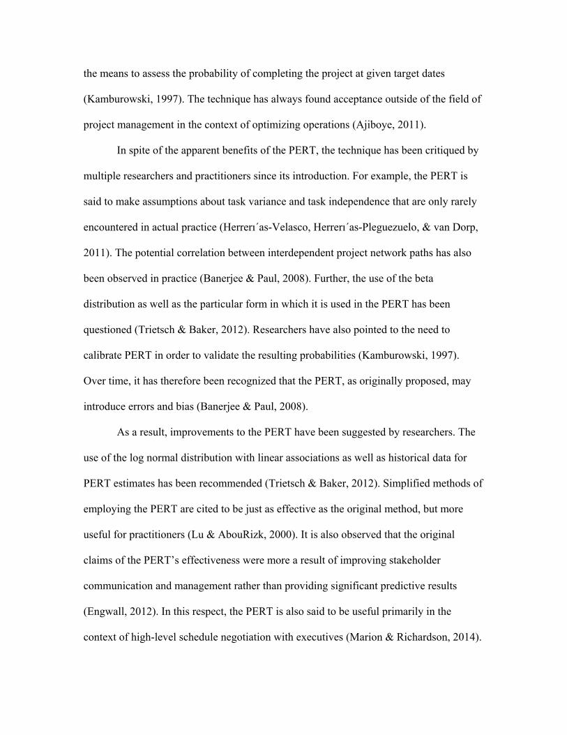
illustrates this fact. This case is based on the Unmanned Aerial Vehicle project (UAV),
“Case 2 UAV.mpp” schedule attached in Appendix 1. The PERT critical path data are
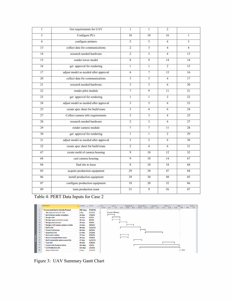
extracted from that file and shown below in Table 4. A summary of the Gantt chart is
illustrated in Figure 3. The probability of completion for the Case 2 schedule will be
calculated for 240 days, 250 days, and 260 days.
Task No. Task Name Optimistic Duration
(O)
Most Likely
Duration (M)
Pessimistic Duration
(P)
Predecessor
0 UAV 242
1 Get requirements for UAV 1 1 2
3 Configure PCs 10 10 16 1
4 configure printers 5 5 6 3
13 collect data for communications 2 3 4 4
14 research needed hardware 2 3 4 13
15 render tower model 8 9 14 14
16 get approval for rendering 1 1 2 15
17 adjust model as needed after approval 6 7 13 16
20 collect data for communications 3 3 4 17
21 research needed hardware 3 3 6 20
22 render pilot module 7 9 11 21
23 get approval for rendering 1 1 2 22
24 adjust model as needed after approval 3 5 6 23
25 create spec sheet for build team 3 4 6 24
27 Collect camera info requirements 2 3 4 25
28 research needed hardware 2 3 6 27
29 render camera module 7 7 11 28
30 get approval for rendering 1 1 2 29
31 adjust model as needed after approval 3 5 6 30
32 create spec sheet for build team 2 4 6 31
67 create mold of camera housing 9 10 12 32
68 cast camera housing 9 10 14 67
84 find site to lease 8 10 18 68
85 acquire production equipment 29 30 47 84
86 install production equipment 29 30 49 85
87 configure production equipment 18 20 32 86
89 train production team 31 9 56 87
Table 4: PERT Data Inputs for Case 2
Figure 3: UAV Summary Gantt Chart

PERT Results for Case 2
Applying the same formulas used for case 1 produces calculated PERT data as
shown in Table 5.
Task No.
Task Name Optimistic Duration (O)
Most Likely Duration (M)
Pessimistic Duration (P)
Predecessor Critical Path Weighted Average durations (t)
Activity Standard Deviation σa
Activity Standard Deviation Squared σa
2
0 UAV 242
1 Get requirements for UAV
1 1 2 1.2 0.17 0.03
3 Configure PCs 10 10 16 1 11.0 1.00 1.00
4 configure printers 5 5 6 3 5.2 0.17 0.03
13 collect data for communications
2 3 4 4 3.0 0.33 0.11
14 research needed hardware
2 3 4 13 3.0 0.33 0.11
15 render tower model 8 9 14 14 9.7 1.00 1.00
16 get approval for rendering
1 1 2 15 1.2 0.17 0.03
17 adjust model as needed after approval
6 7 13 16 7.8 1.17 1.36
20 collect data for communications
3 3 4 17 3.2 0.17 0.03
21 research needed hardware
3 3 6 20 3.5 0.50 0.25
22 render pilot module 7 9 11 21 9.0 0.67 0.44
23 get approval for rendering
1 1 2 22 1.2 0.17 0.03
24 adjust model as needed after approval
3 5 6 23 4.8 0.50 0.25
25 create spec sheet for build team
3 4 6 24 4.2 0.50 0.25
27 Collect camera info requirements
2 3 4 25 3.0 0.33 0.11
28 research needed hardware
2 3 6 27 3.3 0.67 0.44
29 render camera module 7 7 11 28 7.7 0.67 0.44
30 get approval for rendering
1 1 2 29 1.2 0.17 0.03
31 adjust model as needed after approval
3 5 6 30 4.8 0.50 0.25
32 create spec sheet for build team
2 4 6 31 4.0 0.67 0.44
67 create mold of camera housing
9 10 12 32 10.2 0.50 0.25
68 cast camera housing 9 10 14 67 10.5 0.83 0.69
84 find site to lease 8 10 18 68 11.0 1.67 2.78
85 acquire production equipment
29 30 47 84 32.7 3.00 9.00
86 install production equipment
29 30 49 85 33.0 3.33 11.11

87 configure production equipment
18 20 32 86 21.7 2.33 5.44
89 train production team 31 45 56 87 44.5 4.17 17.36
Critical Path Duration (Tcp):
255
Project Standard Deviation (σp):
7.30
Table 5: Calculated PERT data for Case 2
From these data it is possible to calculate via Standard Normal Lookup tables the
probability of finishing the project in 240, 250 and 260 days. These probabilities are
shown in Table 6.
Desired Duration Z Value = (Tdes ‐ Tcp)/σp Probability (P) of Finishing in Desired Duration
240 days ‐2.10 2%
250 days ‐0.73 23%
260 days 0.64 74%
Table 6: PERT calculations for probability of meeting desired schedule durations
Equations 10, 11 and 12 summarize the probability of finishing in 240 days, 250
days, and 260 days, respectively, using the PERT technique.
240 2% Equation 10
250 23% Equation 11
260 74% Equation 12
Monte Carlo Results for Case 2
The MSProject Gantt chart used for Case 2 is included as Appendix 1. The
Monte Carlo analysis results for Case 2 are shown in Figure 4.

Figure 4: Probability histogram for finishing the Case 2 project.
For the purpose of comparing the Monte Carlo and PERT results, it should be
noted that a duration of 240 days correlates to a project finish date of 6/19/15, 250 days
correlates to 7/3/15 and 260 days correlates to 7/17/15. From the histogram in Figure 4
the probability of finishing in those durations is shown in Equations 13, 14 and 15,
respectively.
240 1% Equation 13
250 35% Equation 14
260 90% Equation 15
Comparing the PERT/Monte Carlo simulation Results for Case 2
A comparison of the Monte Carlo simulation results with the PERT results for
Case 2, with a sensitive critical path, shows poor agreement. For the 240 day duration
the PERT prediction is 2% chance of completing on time, while the Monte Carlo
simulation prediction is 1%. The probability of finishing in 250 days is predicted by the

PERT to be 23%, but predicted by Monte Carlo simulation to be 35%. The Monte Carlo
simulation prediction is fully 50% higher than the PERT prediction. For the 260-day
duration the PERT prediction is 74% and the Monte Carlo simulation duration is 90%.
Duration PERT Probability Monte Carlo Probability
240 Days 1% 2%
250 Days 23% 35%
260 Days 74% 90%
Table 7: Summary comparison of PERT vs. Monte Carlo predictions for Case 2.
Concluding remarks
The objective of this paper was to present the findings of the PERT and the Monte
Carlo simulations as schedule risk assessment techniques. We looked at current practice
and used two cases to illustrate the results of each approach using the same data. The
first case used a simple project with an insensitive critical path. The second case, which
better represents a real-world project, is more complex with a sensitive critical path. The
results indicate that the Monte Carlo simulation and the PERT analysis converge only in
the case of a dominant, insensitive critical path. The critical path may appear to be
different when comparing the two methods due to the fact that the PERT uses weighted
average task durations. When the schedule has parallel paths of nearly equal duration,
such that the critical path is very sensitive to activity durations, the PERT method results
begin to diverge from the Monte Carlo simulation results.
We can, therefore, draw a set of conclusions:
1. Conventional PERT network calculations are insufficient, as they do not
adequately account for network sensitivity.

2. Results calculated when using the conventional PERT will usually give a wide
distribution, which reduces the credibility of the calculation.
3. When applying the Monte Carlo simulation, network sensitivity is accounted for
through the numerous iterations of the schedule.
The purpose of this paper was to illustrate the similarities and differences of both
the PERT and the Monte Carlo simulation so project managers and organizations
considering adopting a schedule risk assessment tool are aware of the limitations. In light
of these results, it makes sense that defense contracting reporting requirements were
updated in January 2013 to require Monte Carlo-based Schedule Risk Assessments for all
projects requiring Earned Value Management over $20Million. (Department of Defense,
2013). As a funding authority, the U.S. Department of Defense considers the Monte
Carlo simulation technique a proven risk reduction scheduling practice. It provides
confidence levels for meeting schedule and budget targets and identifies the highest risk
activities affecting the likelihood of meeting schedule and the budget targets.

References
Ajiboye, S. A. (2011). Measuring process effectiveness using Cpm/Pert. International
Journal of Business and Management, 6(6), 286-295. Retrieved from
http://search.proquest.com.ezproxy.libproxy.db.erau.edu/docview/872115911?accou
ntid=27203
Banerjee, A., & Paul, A. (2008). On path correlation and PERT bias. European Journal
of Operational Research, 189(3), 1208-1216.
doi:http://dx.doi.org.ezproxy.libproxy.db.erau.edu/10.1016/j.ejor.2007.01.061
Department of Defense (2013). IPMR Implementation Guide. Retrieved from
http://www.acq.osd.mil/evm/docs/IPMR%20Implementation%20Guide.pdf
Engwall, M. (2012). PERT, polaris, and the realities of project execution. International
Journal of Managing Projects in Business, 5(4), 595-616.
doi:http://dx.doi.org.ezproxy.libproxy.db.erau.edu/10.1108/17538371211268898
Gido, J., & Clements, J. (2014). Successful project management (6th ed.). Boston, MA:
Cengage Learning.
Herrerı´as-Velasco, J. M., Herrerı´as-Pleguezuelo, R., & van Dorp, J. R. (2011).
Revisiting the PERT mean and variance. European Journal of Operational
Research, 210(2), 448-451.
doi:http://dx.doi.org.ezproxy.libproxy.db.erau.edu/10.1016/j.ejor.2010.08.014

Kamburowski, J. (1997). New validations of PERT times. Omega, 25(3), 323-328.
doi:http://dx.doi.org.ezproxy.libproxy.db.erau.edu/10.1016/S0305-0483(97)00002-9
Kerzner, H. (2013). Project management: A systems approach to planning, scheduling,
and controlling (11th ed.). Hoboken, NJ: Wiley.
Kerzner, H. (2010). Project management-best practices: Achieving global excellence
(2nd ed.). Hoboken, NJ: Wiley.
Kwak, Y. H., & Ingall, L. (2007). Exploring monte carlo simulation applications for
project management. Risk Management, 9(1), 44-57.
doi:http://dx.doi.org.ezproxy.libproxy.db.erau.edu/10.1057/palgrave.rm.8250017
Larson, E., & Gray, C. (2014). Project management: The managerial process (6th ed.).
New York, NY: McGraw Hill Higher Education.
Lu, M., & AbouRizk, S. (2000). Simplified CPM/PERT simulation model. Journal of
Construction Engineering and Management, 126(3), 219-226.
doi:10.1061/(ASCE)0733-9364(2000)126:3(219)
Malcolm, D. G., Roseboom, J. H., Clark, C. E., & Fazar, W. (1959). Application of a
technique for research and development program evaluation. Operations research,
7(5), 646-669.
Marion, J. W., & Richardson, T. M. (2014). Using PERT analysis with critical chain
extensions to facilitate information systems project schedule decision-making.
International Journal of Data Analysis and Information Systems, 6(1), 41-47.

Meredith, J., & Mantel, S. (2011). Project management: A managerial approach (8th
ed.). Hoboken, NJ: Wiley.
Project Management Institute. (2012). Practice standard for project risk management.
Philadelphia, PA:
Project Management Institute. (2013). A guide to the project management body of
knowledge (PMBOK guide) (5th ed.). Philadelphia, PA: Project Management
Institute.
Trietsch, D., & Baker, K. R. (2012). PERT 21: Fitting PERT/CPM for use in the 21st
century. International Journal of Project Management, 30(4), 490-502.
doi:http://dx.doi.org.ezproxy.libproxy.db.erau.edu/10.1016/j.ijproman.2011.09.004
Williams, T. (2004). Why monte carlo simulations of project networks can mislead.
Project Management Journal, 35(3), 53-61. Retrieved from
http://search.ebscohost.com/login.aspx?direct=true&db=bth&AN=14780456&site=e
host-live

Appendix 1
“Case 2 UAV.mpp”
Microsoft Project Data File for Case 2
ID Task Name Duration Predecess Finish Successors Early Finish
0 UAV 242 days 5/13/16 5/13/16
1 Get requirements for UAV 1 day 6/11/15 3 6/11/15
2 build Design center computers 22 days 7/13/15 7/13/15
3 Configure PCs 10 days 1 6/25/15 4 6/25/15
4 configure printers 5 days 3 7/2/15 5,13,7 7/2/15
5 Install CATIA (Computer‐Aided Three‐Dimensional
7 days 4 7/13/15 80 7/13/15
6 Design UAV 26 days 8/7/15 8/7/15
7 create computer rendering of UAV on CATIA
10 days 4 7/16/15 8 7/16/15
8 run rendering through software to measure drag
5 days 7 7/23/15 9 7/23/15
9 adjust model as needed 5 days 8 7/30/15 10 7/30/15
10 get approval for rendering 1 day 9 7/31/15 11 7/31/15
11 adjust model as needed after approval
5 days 10 8/7/15 34,35,78,80, 8/7/15
12 Design communications tower 26 days 8/7/15 8/7/15
13 collect data for communicatio3 days 4 7/7/15 14 7/7/15
14 research needed hardware 3 days 13 7/10/15 15 7/10/15
15 render tower model 9 days 14 7/23/15 16 7/23/15
16 get approval for rendering 1 day 15 7/24/15 17 7/24/15
17 adjust model as needed after approval
7 days 16 8/4/15 18,20 8/4/15
18 create spec sheet for build te 3 days 17 8/7/15 61,78,80 8/7/15
19 Design pilot controls 25 days 9/8/15 9/8/15
20 collect data for communicatio3 days 17 8/7/15 21 8/7/15
21 research needed hardware 3 days 20 8/12/15 22 8/12/15
22 render pilot module 9 days 21 8/25/15 23 8/25/15
23 get approval for rendering 1 day 22 8/26/15 24 8/26/15
24 adjust model as needed after approval
5 days 23 9/2/15 25 9/2/15
25 create spec sheet for build te 4 days 24 9/8/15 78,80,27 9/8/15
26 Design multi camera system mo23 days 10/9/15 10/9/15
27 Collect camera info requirem3 days 25 9/11/15 28 9/11/15
28 research needed hardware 3 days 27 9/16/15 29 9/16/15
29 render camera module 7 days 28 9/25/15 30 9/25/15
30 get approval for rendering 1 day 29 9/28/15 31 9/28/15
31 adjust model as needed after approval
5 days 30 10/5/15 32 10/5/15
project Manager
IT department
IT department
IT department
UAV Design team
UAV Design team
UAV Design team
UAV Design team
UAV Design team
Tower Design team
Tower Design team
Tower Design team
Tower Design team
Tower Design team
Tower Design team
Control Design team
Control Design team
Control Design team
Control Design team
Control Design team
Control Design team
Camera design team
Camera design team
Camera design team
Camera design team
Camera design team
S T M F T S W S T M F T S W S T M F T S W S T M F T S W S T M F5 Jun 7, '15 Jul 5, '15 Aug 2, '15 Aug 30, '15 Sep 27, '15 Oct 25, '15 Nov 22, '15 Dec 20, '15 Jan 17, '16 Feb 14, '16 Mar 13, '16 Apr 10, '16 Ma

ID Task Name Duration Predecess Finish Successors Early Finish
32 create spec sheet for build te 4 days 31 10/9/15 78,80,67,66 10/9/15
33 Build UAV 68 days 11/11/15 11/11/15
34 acquire needed supplies for U8 days 11 8/19/15 37 8/19/15
35 buy parts for UAV build 8 days 11 8/19/15 37 8/19/15
36 create prototype for molding 30 days 9/30/15 9/30/15
37 Build fuselage 10 days 35,34 9/2/15 38 9/2/15
38 build wings 10 days 37 9/16/15 39 9/16/15
39 build tail 10 days 38 9/30/15 41 9/30/15
40 cast mold 30 days 11/11/15 11/11/15
41 create mold of fuselage 10 days 39 10/14/15 42 10/14/15
42 create mold of wings 10 days 41 10/28/15 43 10/28/15
43 create mold of tail 10 days 42 11/11/15 45 11/11/15
44 Create final pieces 16 days 12/3/15 12/3/15
45 make and sand wings 2 days 43 11/13/15 46 11/13/15
46 make and sand fuselage 7 days 45 11/24/15 47 11/24/15
47 make and sand tail section 7 days 46 12/3/15 49,80 12/3/15
48 assemble UAV 57 days 2/22/16 2/22/16
49 attach wings 10 days 47 12/17/15 50 12/17/15
50 attach tail 7 days 49 12/28/15 51 12/28/15
51 install motor 5 days 50 1/4/16 52 1/4/16
52 install communications radio 8 days 51 1/27/16 53 1/27/16
53 install camera 9 days 52 2/9/16 54 2/9/16
54 install pilot controls 9 days 53 2/22/16 71,72,73,74, 2/22/16
55 build pilot station 27 days 9/15/15 9/15/15
56 Acquire hardware 8 days 11 8/19/15 57 8/19/15
57 assemble station 7 days 56 8/28/15 58 8/28/15
58 load UAV pilot software 6 days 57 9/7/15 59 9/7/15
59 Configure UAV software 6 days 58 9/15/15 71,72,73,74, 9/15/15
60 Build communications tower 26 days 9/14/15 9/14/15
61 acquire hardware 5 days 18 8/14/15 62 8/14/15
62 assemble station 10 days 61 8/28/15 63 8/28/15
63 Install ArduPilot Mega (APM) 6 days 62 9/7/15 64 9/7/15
64 Setup five‐channel RC Radio 5 days 63 9/14/15 71,72,73,74, 9/14/15
65 Build removable camera assemb27 days 11/17/15 11/17/15
66 acquire hardware 5 days 32 10/16/15 69 10/16/15
67 create mold of camera housin10 days 32 10/23/15 68 10/23/15
68 cast camera housing 10 days 67 11/6/15 69,84,88 11/6/15
69 assemble camera 7 days 68,66 11/17/15 71,72,73,74, 11/17/15
70 Test UAV 40 days 4/18/16 4/18/16
Camera design team
purchasing agent
UAV Build parts[1]
UAV Build team
UAV Build team
UAV Build team
UAV Build team
UAV Build team
UAV Build team
UAV Build team
UAV Build team
UAV Build team
UAV Build team
UAV Build team
UAV Build team
UAV Build team
UAV Build team
UAV Build team
pilot station hardware[1]
pilot station build team
pilot station build team
pilot station build team
Communications tower hardware[1]
Communications tower build team
Communications tower build team
Communications tower build team
Camera assembly hardware[1]
Camera build team
Camera build team
Camera build team
S T M F T S W S T M F T S W S T M F T S W S T M F T S W S T M F T S W S T M F5 Jun 7, '15 Jul 5, '15 Aug 2, '15 Aug 30, '15 Sep 27, '15 Oct 25, '15 Nov 22, '15 Dec 20, '15 Jan 17, '16 Feb 14, '16 Mar 13, '16 Apr 10, '16 May 8, '16 Jun 5, '16 Jul 3, '16 J
71 Test Battery Life 30 days 54,59,64, 4/4/16 76 4/4/16
72 Test Weather Conditions 30 days 54,59,64, 4/4/16 76 4/4/16
73 Test Range 30 days 54,59,64, 4/4/16 76 4/4/16
74 Test Communications Interfer30 days 54,59,64, 4/4/16 76 4/4/16
75 Measure avg. Pilot training Le7 days 54,59,64, 3/2/16 76,80 3/2/16
76 document test findings 10 days 71,72,73, 4/18/16 90 4/18/16
77 Create UAV documentation 151 days 5/9/16 5/9/16
78 Technical publications 14 days 11,18,25, 10/29/15 79,82 10/29/15
79 Engineering Data 14 days 78 11/18/15 82 11/18/15
80 Management Data 14 days 11,18,25, 3/22/16 81,82 3/22/16
81 Support Data 14 days 80 4/11/16 82 4/11/16
82 Build Data Repository 20 days 78,79,80, 5/9/16 90 5/9/16
83 Full Production site 135 days 5/13/16 5/13/16
84 find site to lease 10 days 68 11/20/15 85 11/20/15
85 acquire production equipmen30 days 84 1/1/16 86 1/1/16
86 install production equipment30 days 85 2/12/16 87 2/12/16
87 configure production equipm20 days 86 3/11/16 89 3/11/16
88 hire full production team 30 days 68 12/18/15 89 12/18/15
89 train production team 45 days 88,87 5/13/16 90 5/13/16
90 Begin Production 0 days 89,82,76 5/13/16 5/13/16
test team 1
test team 2
test team 3
test team 4
test team
documentation team
documentation team
documentation team
documentation team
documentation team
documentation team
site lease[1]
production equipment[1]
Contractor
Contractor
management team
training team
5/13