a comparative analysis of contact metrology devices … · a comparative analysis of contact...
TRANSCRIPT

A Comparative Analysis Of Contact Metrology Devices Versus Non-Contact Metrology
Systems Utilizing Structured Light
by
Michael Hestness
A Research Paper Submitted in Partial Fulfillment of the
Requirements for the Master of Science Degree
in
Manufacturing Engineering
The Graduate School
University of Wisconsin-Stout
December 2011
Copyright 2011 Lockheed Martin

2
Copyright 2011 Lockheed Martin
The Graduate School University of Wisconsin-Stout
Menomonie, WI 54751
Author: Hestness, Michael L.
Title: A Comparative Analysis of Contact Metrology Devices versus Non-
Contact Metrology Systems Utilizing Structured Light
Graduate Degree/ Major: Master of Science in Manufacturing Engineering
Research Adviser: John Dzissah
Month/Year: December, 2011
Number of Pages: 86
Style Manual Used: American Psychological Association, 6th
edition
Abstract
Modern aerospace manufacturing processes utilize the most advanced techniques
and technologies in the world. The need for lower cost and more efficient aircraft is
pushing the limits of current material and process capabilities. In an effort to meet these
requirements, aircraft designs require tighter tolerances than ever to ensure quality,
safety, and performance. While this may result in efficient airplanes with lower
operating costs, the initial costs to manufacture parts meeting stringent tolerances and
the subsequent inspection methods drive up production costs.
To meet these challenges, improved manufacturing and inspection techniques
are required. Traditionally, coordinate measuring machines (CMMs) and laser trackers
have been the metrology workhorses of aerospace. While these technologies are
accurate, they are slow and can be labor intensive to program and operate. Recent

3
Copyright 2011 Lockheed Martin
advances in non-contact inspection technologies such as white light, or structured light,
have produced impressive results but there is limited data to demonstrate these
technologies are as accurate as the legacy methods. This paper will compare the
capability of three white light systems to the capability of contact metrology
measurement devices by conducting a gage linearity and bias study and a gage
repeatability and reproducibility study for each white light scanning system.

4
Copyright 2011 Lockheed Martin
The Graduate School
University of Wisconsin Stout Menomonie, WI
Acknowledgments
I would like to thank my wife Amy and our kids for their support and patience
during my time in school. I would also like to thank the faculty of UW-Stout, especially
David Fly, for the support he and everyone has provided to me as a distance learning
student. Last but not least, I would like to thank Dr. John Dzissah for his time and
guidance completing this paper.

5
Copyright 2011 Lockheed Martin
Table of Contents
.................................................................................................................................. Page
Abstract ........................................................................................................................... 2
List of Tables ................................................................................................................... 7
List of Figures .................................................................................................................. 8
Chapter I: Introduction ..................................................................................................... 9
Statement of the Problem ................................................................................... 11
Purpose of the Study .......................................................................................... 12
Assumptions of the Study ................................................................................... 13
Limitations of the Study ...................................................................................... 13
Definition of Terms ............................................................................................. 14
Methodology ....................................................................................................... 15
Chapter II: Literature Review ......................................................................................... 17
Early Metrology Tools ......................................................................................... 17
Coordinate Measuring Machines ........................................................................ 19
Non-Contact Metrology ....................................................................................... 22
Gage Repeatability and Reproducibility .............................................................. 26
The Future of Non-contact Inspection ................................................................ 27
Chapter III: Methodology ............................................................................................... 28
Equipment .......................................................................................................... 28
Features and Test Articles .................................................................................. 32
Benchmarking ..................................................................................................... 35

6
Copyright 2011 Lockheed Martin
Non-contact Data Collection ............................................................................... 36
Gage Repeatability and Reproducibility Study ................................................... 44
Chapter IV: Results ....................................................................................................... 45
Results ............................................................................................................... 45
Summary of Findings .......................................................................................... 45 Gage Linearity and Bias Study ........................................................................... 46 Gage Repeatability and Reproducibility Study ................................................... 47
Chapter V: Discussion ................................................................................................... 50
Conclusions ........................................................................................................ 50
Recommendations .............................................................................................. 50
References .................................................................................................................... 52
Appendix A: Spot Face Panel Drawing ........................................................................ 55
Appendix B: Spot Face Panel Benchmark Results ....................................................... 56
Appendix C: Countersink Test Coupon Dimensions ..................................................... 57
Appendix D: Precision Surface Block ............................................................................ 58
Appendix E: Two-Ball, Ball Over Method Formula ........................................................ 59
Appendix F: Input Data and Results for Precision Surface Panel ................................. 60
Appendix G: Input Data and Results for Spot Face Panel ............................................. 69
Appendix H: Input Data and Results for Countersink Panel .......................................... 78
.
7
Copyright 2011 Lockheed Martin
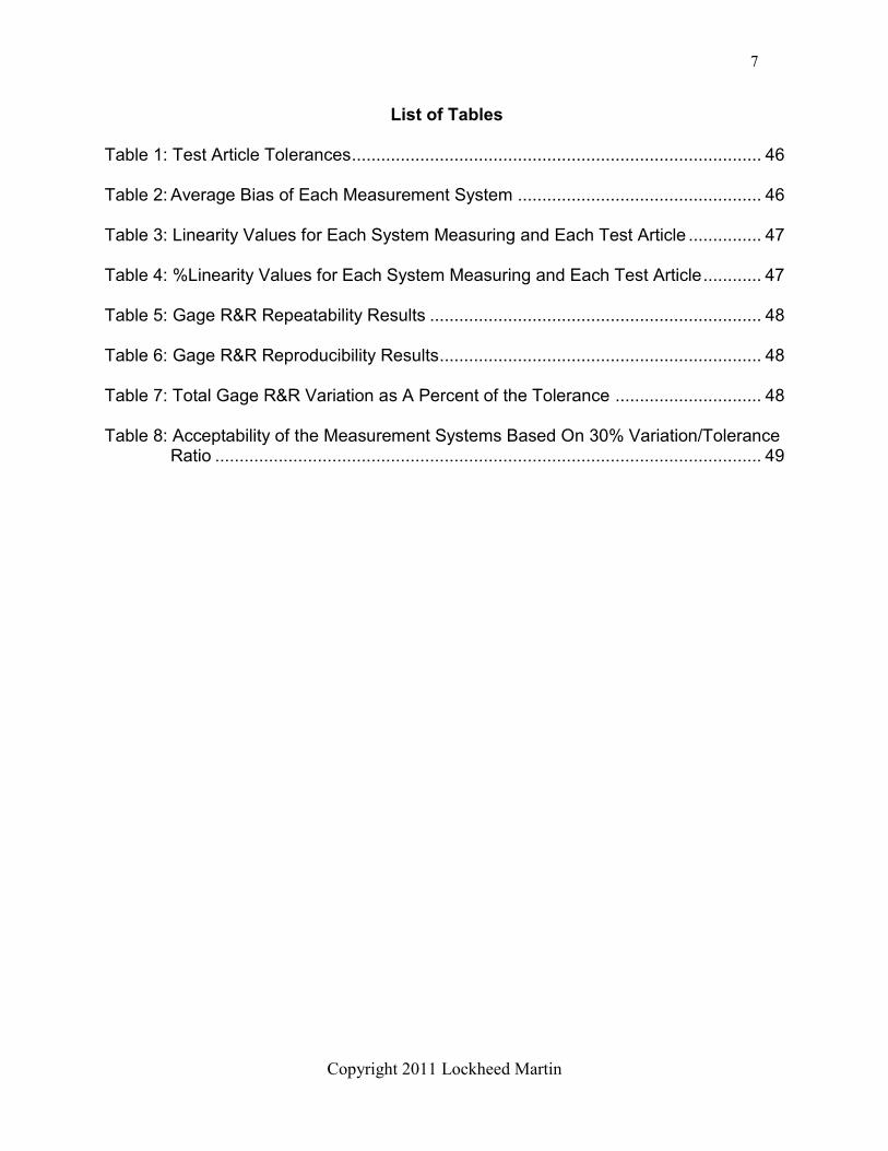
List of Tables Table 1: Test Article Tolerances .................................................................................... 46 Table 2: Average Bias of Each Measurement System .................................................. 46 Table 3: Linearity Values for Each System Measuring and Each Test Article ............... 47 Table 4: %Linearity Values for Each System Measuring and Each Test Article ............ 47 Table 5: Gage R&R Repeatability Results .................................................................... 48 Table 6: Gage R&R Reproducibility Results .................................................................. 48 Table 7: Total Gage R&R Variation as A Percent of the Tolerance .............................. 48 Table 8: Acceptability of the Measurement Systems Based On 30% Variation/Tolerance
Ratio ................................................................................................................ 49

8
Copyright 2011 Lockheed Martin
List of Figures
Figure 1: Micrometer ..................................................................................................... 18 Figure 2: Vernier caliper ................................................................................................ 19
Figure 3: Zeiss Accura II AKTIV CMM ........................................................................... 29 Figure 4: CogniTens WLS 400M ................................................................................... 30 Figure 5: ATOS Triple Scan .......................................................................................... 31 Figure 6: Rexcan 4 White Light Scanner ....................................................................... 32 Figure 7: Precision Surface Block ................................................................................. 33 Figure 8: Spot Face Panel ............................................................................................. 34 Figure 9: Countersink Panel .......................................................................................... 35 Figure 10: Calibrating the WLS 400M ........................................................................... 37 Figure 11: Measuring the Precision Surface Block with the WLS 400M ........................ 38 Figure 12: Measuring the Spot Face Panel with the WLS 400M ................................... 38 Figure 13: Measuring the Countersink Panel with the WLS 400M ................................ 39 Figure 14: Calibrating the Rexcan 4 .............................................................................. 40 Figure 15: Mapping the Artifact with Photogrammetry................................................... 40 Figure 16: Measuring the Precision Surface Block with the Rexcan 4 ......................... 41 Figure 17: Measuring the Spot Face Panel with the Rexcan 4 ...................................... 41 Figure 18: Measuring the Countersink Panel with the Rexcan 4 ................................... 42 Figure 19: Measuring the Precision Surface Block with the ATOS Triple Scan ............. 42 Figure 20: Measuring the Spot Face Panel with the ATOS Triple Scan ........................ 43 Figure 21: Measuring the Countersink Panel with the ATOS Triple Scan ..................... 43

9
Copyright 2011 Lockheed Martin
Chapter I: Introduction
Many of today’s products have been designed with manufacturing tolerances that
were unachievable just ten years ago. As modern manufacturing processes improve
and become capable of producing these extremely precise parts, it becomes imperative
to have methods of inspection that are precise and capable of rapidly inspecting these
parts.
The automotive and aerospace industries have typically been the main users of
very precise and highly inspected parts. Components in an engine, whether it is an
automotive engine or a jet engine, are often held to tolerances in the ten thousandths of
an inch range. To measure these parts accurately, coordinate measuring machines
(CMMs) have long been considered a gold standard in metrology, which is the study of
measurements. A CMM is a measurement device used to make three-dimensional
measurements (Kalpakjian, 1992) and can come in several forms, but a typical bridge
CMM consists of a granite bed, a touch probe, and a gantry system allowing very
precise control of the touch probe in three axes.
As the aerospace industry develops larger aircraft with increasingly tight
tolerances to achieve the desired performance, the need to build larger CMMs becomes
clear. These new CMMs are very expensive because as the inspection volume
increases, so does the cost. Many CMMs used in aerospace are housed in
environmentally controlled buildings. Larger CMMs require larger buildings and more
controls to maintain a constant room temperature. Also, as the machines become
larger they need to be made more rigid and sit on sturdier foundations.

10
Copyright 2011 Lockheed Martin
A long Y-axis bridge is more susceptible to bending and vibrations than a short
bridge. In addition, the further the CMM travels from its home or start position (x=0,
y=0, z=0), the more likely it is to lose accuracy. To compensate for this, large CMMs
need better encoders and specialized software to ensure they remain accurate over a
large volume.
Lockheed Martin is producing the F-35 Joint Strike Fighter and is expected to
produce one plane per day when full rate production is realized. As the only 5th
generation fighter jet in production, no other airplane in the world is manufactured to the
stringent tolerances required to ensure the plane meets its performance goals. A 5th
generation plane is considered a low observable (LO) plane and is more commonly
known as a stealth plane. LO planes are designed to be nearly invisible to radar. To
achieve LO performance, the plane utilizes unique shape characteristics, advanced
materials, and special coatings. All of these must be strictly controlled and verified.
The use of the digital thread (Kinard, 2010) has also added to the challenges of
aerospace manufacturing. Coined by Lockheed Martin, the term digital thread means
there are no master tools used to build parts. Every part produced is controlled by a
three-dimensional computer model. Legacy aircraft started with engineering drawings,
but those drawings were turned into gage tools that superseded the drawings. Once
parts were produced they could always be compared back to the gage tools if there was
a problem with the way that parts fit to the aircraft. Legacy aircraft also used drill
fixtures and routing jigs to shape parts and drill holes. With the digital thread, the hard
tooling is gone.

11
Copyright 2011 Lockheed Martin
While the benefits of the digital thread outweigh the challenges associated with it,
when there is a problem with components fitting together during the assembly process it
now becomes very difficult to tell which part is out of tolerance. This leads to the need
to inspect large assemblies such as landing gear doors, hinge assemblies, and aircraft
door openings. Measuring components like this is not something CMMs were ever
intended to do and even if an assembly such as a landing gear door was fixtured to a
CMM bed, it would take far too long to inspect enough points to get to the root cause of
the part mismatch. This has led to the development of new non-contact inspection
methods such as coherent laser radars, structured white light, and laser scanners.
While these new systems are developing rapidly, there is limited data supporting that
the accuracy of these systems is comparable to traditional CMMs. The advantage to
these non-contact systems is they are portable, much less expensive, record millions of
data points in a matter of seconds, and do not require labor intensive numerical control
programming.
While the coordinate measuring machine will retain its need in industry for a long
time to come, there is an urgent need to advance and validate the capabilities of non-
contact inspection methods in the manufacturing world.
Statement of the Problem
Coordinate measuring machines utilizing touch-probes are capable of recording
very accurate and precise measurements, but they are expensive, take up valuable
floor space, are sensitive to vibration, and only collect one point at a time; they are not
considered to be a rapid inspection technology. Non-contact inspection technologies

12
Copyright 2011 Lockheed Martin
exist that may provide solutions to these challenges, but there is limited data to support
that the non-contact systems are as accurate as touch-probe CMMs.
Purpose of the Study
The purpose of this study is to quantify the accuracies of non-contact metrology
systems utilizing structured light. Coordinate measuring machines are considered to be
one of the most capable metrology instruments available (Chapman, 2002), and are
traceable to the National Institute of Standards and Technology (NIST) standards
(Morey, 2010a), however, they are not without limitations. They require dedicated floor
space, computer programs to run them, special fixturing for the parts to be inspected,
are sensitive to vibrations, and only record a single data point each time they touch a
part. Although touch probes are capable of recording up to 60 points per minute
(Chapman, 2002), this is not fast enough for certain manufacturing applications.
Non-contact technology utilizing structured light technology, commonly referred
to as white light technology, uses a light source to project a two-dimensional shadow
pattern on a three-dimensional surface. Digital cameras then record the distorted image
that result from the contours and features of the three-dimensional surface. Powerful
software takes this image and calculates the distance the cameras are from the surface
and thus measures the part. Some of the newer systems now use blue light-emitting-
diodes (LEDs) to produce the two dimensional pattern. Advantages of blue light will be
discussed later.
According to Marc Demarest (Morey, 2010a), structured light technology has
been around since 1995, so this isn’t new technology. However, it has been gaining
13
Copyright 2011 Lockheed Martin
notoriety and feels like new technology to many users. As with any technology that is
new to a user, it is important to establish a baseline for the current state of the art and
then qualify the new technology to existing standards ensuring equivalency of
performance.
The deliverables of this study consist of gage linearity and bias study validating
the accuracy of the structured light measurement systems, and a gage repeatability and
reproducibility (gage R&R) study validating the robustness of the measurement process.
Assumptions of the Study
Gage R&R studies were not conducted on the contact metrology devices. The
CMM was calibrated in compliance with DIN EN ISO 10360-2:2001 on January 26,
2011and was accurate within 3 microns/meter. The Fowler height gage was within the
calibration certification date and verified with a NIST traceable standard. The two-ball-
over method used to measure the countersinks is considered an acceptable method of
calibrating countersink gages at Lockheed Martin.
Minitab gage R&R results no longer utilize 5.15 standard deviations to calculate
gage variation. Minitab 16 calculates study variation as 6 times the standard deviation
of each variation source in accordance with recommendations from the Automotive
Industry Action Group (AIAG) (Minitab Inc, 2010).
Limitations of the Study
This study was limited by several factors. The amount of time the CMM was
available to measure and baseline the test artifacts meant that test artifacts had to be
selected with measurement capacity in mind. Two artifacts that had originally been
scoped had to be eliminated from testing because the large CMM required to measure

14
Copyright 2011 Lockheed Martin
them was not available. CMM programmer time also affected the selection of artifacts.
Due to the lack of CMM capacity, a gage R&R was not performed for any of the contact
measurement processes. The artifact measured on the CMM was only measured once,
as was the case for the spot face panel and the countersink panel. Budget constraints
had an effect on the number of white light scanners tested and a reduction in manpower
lead to down-scoping the original project.
The time it took to analyze the data was also a limiting factor in this study. While
collecting data can be accomplished relatively quickly, analyzing point cloud data can
take a considerable amount of time. Once the process of isolating the desired features
from rest of the point cloud has been defined, an algorithm can be developed to
automate the process. However, defining the initial process can be time consuming and
may require multiple algorithms for features such as varying hole diameters.
Definition of Terms
Benchmark. “A standard by which something can be measured or judged”
(“Benchmark,” n.d., para. 1).
Bias. The difference between the measured point and the reference point
(Minitab, 2010)
Bridge-type CMM. “A type of CMM with a horizontal beam holding the probe.
The bridge-type CMM is the most common type” (“Basics,” 2011, para. 3).
Calibrated. When an instrument is compared to a more accurate instrument to
indentify and correct measurement errors (Goldsmith, 2010).

15
Copyright 2011 Lockheed Martin
Coordinate measuring machine. “A sophisticated measuring instrument with a
flat polished table and a suspended probe that measures parts in three-dimensional
space” (“Basics,” 2011, para. 3).
Digital thread. “Digital thread implies that 3D exact solid models from
engineering design are used directly by manufacturing for NC programming, coordinate
measurement machines inspections, and tooling (which are also 3D solid models)”
(Kinard, 2010, para 3).
Gage repeatability and reproducibility. Also know as gage R&R, it is a study
to “determine the magnitude of the variation in a measurement system as well as the
sources of this variation” (Kappele and Raffaldi, 2005, para 2).
Linearity. Linearity is an expression of the accuracy of the gage throughout the
expected range of measurements (Minitab, 2010)
Metrology. “The science that deals with measurement” (“Metrology,” n.d., para.
1).
Micron. One millionth of one meter. (“Micron,” n.d., para. 1).
Structured light. A pattern of light projected from either a white light source or a
blue light source onto a three dimensional surface (Morey, 2010).
Traceable. The ability to connect a measurement to a national or international
standard through an unbroken set of comparisons (Goldsmith, 2010).
Methodology
The researcher conducted a gage linearity and bias study for three structured
white light systems and compared them to contact metrology methods including a Zeiss

16
Copyright 2011 Lockheed Martin
Accura II AKTIV CMM, a Fowler digital indicator (Model 54-520-777) attached to a
height gage, and a two-ball-over method of measurement. Three test articles were
benchmarked with the contact measurement methods and then measured with a
CogniTens WLS400M Blue Light Scanner, a GOM ATOS Triple Scan with Blue Light
Technology, and a Rexcan 4 white light scanner by Solutionix. In addition to performing
the gage linearity and bias study to validate accuracy, a gage repeatability and
reproducibility (gage R&R) study was conducted. The gage R&R utilized three different
operators to measure the three test articles, each containing twenty-one measurement
points/features. Each operator measured each article three times. The results of the
gage R&R were evaluated with Minitab 16.0.0 software using the ANOVA method.

17
Copyright 2011 Lockheed Martin
Chapter II: Literature Review
As manufacturing technologies mature, and design engineers create larger and
more complex structures, the need for improved inspection technologies becomes
increasingly important. Traditional inspection equipment and processes are capable of
performing very accurate and very precise measurements, but these processes are
often relatively slow and very expensive. In addition, these processes only inspect
discrete points that may not fully reflect the condition of the part. When analyzing why
parts do not fit together properly in an assembly it is helpful to have surface data rather
than single point inspection data. A cloud of surface points may reveal a wavy, uneven
surface while the individual points gathered from a traditional CMM may be coincidently
spaced such that they reveal a near perfectly flat surface.
Three-dimensional non-contact inspection technologies have been in use for
over fifteen years but they are just now becoming capable of meeting the high accuracy
and high precision requirements of modern manufacturing industries such as
automotive and aerospace (Morey, 2010a). As a result of improving capability there is a
rush to refine and utilize these technologies to reduce manufacturing costs as well
increase manufacturing throughput. This chapter will review the current body of
literature and discuss early metrology tools, coordinate measuring machines, non-
contact metrology systems used in industry, gage repeatability and reproducibility, and
finally comments on the future of non-contact metrology.
Early Metrology Tools
The need for standard measurement devices has existed for nearly all of history
(Bucher, 2004). Methods of measuring distance were often a function of a body part

18
Copyright 2011 Lockheed Martin
such as the length of an arm or the width of a hand. Time was measured by cycles of
the sun, the moon, and the appearance of specific stars. Standard methods of
measuring food and liquids were required for cooking and bartering.
According to Bucher (2004), the use of calibrated and traceable measurement
standards goes as far back as the Egyptians. The royal cubit was made from granite
and was used as the official measurement standard. From this standard, additional
cubits were made of wood and then used in construction throughout the land. To
ensure the accuracy of the wooden cubits used by the workers, at each full moon the
cubits were returned to the royal architect and compared to the royal cubit. The
punishment for failing to return a wooden cubit was death. Because the Egyptians had
this strict system of standards they were able to build the Great Pyramid of Giza to an
accuracy of 4 ½ inches over 756 feet.
Brown and Sharpe introduced the first micrometer to the public in 1867 (Roe,
1916). While they had been in use by machinists before this time, this marked the first
time it was produced in mass. A micrometer is a handheld device consisting of a frame,
anvil, sleeve, spindle, thimble and a ratchet (Figure 1). Modern micrometers are
considered to be very precise and are accurate to ± .00005 in. (Starrett, 2011a).
Figure 1. Micrometer. Retrieved from http://www.technologystudent.com/equip1/microm1.htm

19
Copyright 2011 Lockheed Martin
While not as precise or accurate as a micrometer, another extremely useful hand
tool is the vernier caliper (Figure 2). Calipers can measure external features, internal
features, and depths to an accuracy of ±.0001 in. (Starrett, 2011b).
Figure 2. Vernier caliper. Retrieved from http://www.technologystudent.com/equip1/vernier3.htm
There are many useful hand tools available to machinists to make extremely
accurate and precise measurements, but for many of the manufacturing processes
employed today, hand tools are not adequate (Logee, Fabiano, & Cassola, 2009).
Whether it is the potential of human error, the number of points being inspected, or
shape of the part, many times automation in metrology is required.
Coordinate Measuring Machines
The coordinate measuring machine (CMM) has long been considered the
standard in metrology (O’Rourke, 2011). CMMs have been in existence since the
1960’s but have been continually improved and enhanced. According to Mark Bliek of
Bolton Works, “CMMs are still the workhorses for geometric quality control. The
calibration of a CMM can be traced back to NIST standards, and therefore the industry
is comfortable with the measurements made with a CMM” (Morey, 2010a, p.57).
Bucher (2004) says that using traceable standards for calibration is essential to
ensuring consistent parts. Using a traceable standard means that any measurement
standard used in the calibration of a measurement device can be verified by a more

20
Copyright 2011 Lockheed Martin
accurate measurement standard which can be compared to a master standard held by
an organization such as NIST. There has to be an unbroken chain of verification from
the master NIST standard down to the final equipment being calibrated. This does not
mean a machinist has to send their micrometer to NIST for calibration, but the
measurement standard they use must have been inspected by a more accurate
measurement standard that is traceable to a NIST standard. The use of a single master
measurement standard ensures that a .5 in. bolt in the United States is the same as a .5
in. bolt in Germany. This is ensured by the Bureau International des Poids et Mesures
(BIPM) in Sevres, France providing all countries with the same defined standards.
Originally CMMs were two-axis, manually driven machines. However, modern
CMMs are now computer controlled and have up to five axes or degrees of freedom
(Morey, 2010b). To ensure the CMM is performing as expected, there are several
standards that may be used to calibrate the CMM. ISO 10360-2, ASME B89.4.10360.2-
2008, and VDI/VDE 2617 are the most common standards used today (Card, 2003).
These standards are similar to each other, but they each specify a different number of
tests and different procedures for performing these tests. Over the years these
documents have adopted similar procedures to truly become standardized in areas
such as environmental controls. ISO 10360-2 used to require testing at specific
temperatures, but now just as in ASME B89.4.10360.2-2008 the user is free to choose
the environmental conditions. Nevertheless, in spite of the variations in these
documents, all standards require traceability to NIST artifacts or standards making the
CMM a highly regarded tool in metrology.
21
Copyright 2011 Lockheed Martin
CMMs come in a wide range of sizes, shapes and configurations (O’Rourke,
2011). There are small bench top CMMs that are still hand driven as well as ones that
have linear drive motors and digital readouts to make it easier to record measurements.
There are portable CMMs such as arms. The Faro Edge ScanArm weighs 24 pounds
and can be mounted to a bench top or movable stand. Mraz (2011) says the Faro arm
comes in three models that have working envelope ranges of 6 ft, 9 ft, and 12 ft. The 6
ft model has a stated single-point repeatability of .0009 in. while the 12 ft model is
repeatable to .0025 in. This means an operator measuring the same point two times
with the 6 ft model can find the same point to an accuracy of .0009 in. In addition to the
bench top and portable models, companies like Lockheed Martin have CMMs with
machine beds that that are 16 meters long, 5 meters wide, and capable of measuring
parts 2.5 meters tall with a linear accuracy of 10 microns per meter (B. Kush, personal
communication, August 1, 2011).
Coordinate measuring machines are very accurate and useful for measuring
parts, but each part measured requires its own computer program to run the machine.
Some parts may only take a couple of hours to program but Mark Boucher (2007) of
NewCastle Measurement says developing CMM a program for an extremely complex
part could take several days to complete. In addition to the lengthy programming time
the CMM also may require numerous calibration routines to be developed to account for
and reduce the risk of probe offset errors. Programming can often be performed off line
which saves CMM time, but still requires the expense of a CMM programmer. Software
is constantly being improved to make programming easier, but often the CMM programs
are not compatible with CMMs from different manufacturers. This means if a shop has

22
Copyright 2011 Lockheed Martin
multiple CMMs from different manufacturers, the CMMs must have dedicated parts or
multiple programs will be required. CMMs are very useful, but not always flexible and
accommodating to change.
Non-Contact Metrology
As the automotive, aerospace, and wind turbine industries move forward with
more advanced designs and manufacturing processes, it becomes clear that even
though the CMM will not be disappearing anytime soon, new methods of inspection will
be required. The aerospace industry and the wind turbine industry both use very large
monolithic composite structures. According to Zach Rodgers at Nikon Metrology,
whether it is a barrel section of a commercial plane’s fuselage, or a long wind turbine
blade, measuring large structures like these is just not feasible with a CMM (Morey,
2011, p. 59-60). In both automotive and aerospace there is a need to rapidly inspect
complex shapes that would be impractical to fixture on a CMM (Morey, 2010b). To
measure parts in this complex environment, the need for non-contact inspection
technologies is rapidly growing.
In 2004, Lockheed Martin Aeronautics determined they had to develop an
alternative approach to controlling the thickness of composite wing skins (P. Briney,
personal communication, July 7, 2011). Lockheed’s previous approach utilized very
expensive milling machines to profile the inner mold line of the laminate which left
structurally unnecessary material on the part resulting in excessive weight. To
overcome this challenge, the cured laminate compensation (CLC) process was
developed. The CLC process was made possible through the use of the Nikon MV-224
Coherent Laser Radar (CLR).

23
Copyright 2011 Lockheed Martin
The MV-224 is a form of non-contact CMM and has been replaced by the next
generation Nikon MV-330. Originally developed by Coleman Research in the early
1990’s, the laser radar has been in continual use and undergoing improvements ever
since (P. Morken, personal communication, July 7, 2011). According to the Nikon Laser
Radar Training Workbook (2010) the MV330 operates on a principle similar to the
conventional radar principle of time-of-flight. To do this, a laser beam is split into two
beams with one beam traveling through a reference coil of known length and the other
beam traveling to the surface. Distance is calculated by measuring the time it takes for
the laser signal to reflect back from the surface being measured, and comparing this
signal to the time it takes the second signal to travel though the reference coil. Since
time-of-flight can be difficult to measure, the laser signal is modulated to vary its
frequency. The change in the frequency has a direct relationship to time-of-flight and is
much easier to measure. It is through the development of proprietary software that
Nikon has been able to achieve this. The MV-330 has a stated accuracy of .001 in. at a
distance of 6 ft, and .004 in. at 100 ft. It was this level of accuracy and the
programmable non-contact features that enabled Lockheed Martin to develop a solution
to their composite thickness challenge. The Laser Radar can be operated in a manual
mode or programmed just like the touch-probe CMMs, enabling them to consistently
measure the same discrete points. Jeff Drewett of Lockheed Martin says the CLR
makes the CLC process repeatable to .0013 in. on composite surfaces and .0008 in. on
an Invar cure tool surface (Morey, 2011, p. 63).
The latest technology to make headlines in metrology is structured light.
Structured light is not a new technology, but it has gained notoriety in the last couple of

24
Copyright 2011 Lockheed Martin
years (Morey, 2011). It is commonly referred to as white light scanning even with the
recent introduction of blue light scanners. Hexagon Metrology has unveiled a new
scanner utilizing blue light-emitting-diodes (LEDs) as the light source, but they branded
the product as the WLS400 to take advantage of the white light name.
The terms white light system and structured light system have become a sort of
catch-all for several technologies (3D Surface Reconstruction Technologies, 2008).
Currently there are systems utilizing white light and systems using blue light. White light
was the first to be developed, but white light systems can be affected by shiny surfaces.
Blue light scanners filter out all wave-lengths except blue light, and are therefore less
sensitive to ambient light and highly reflective surfaces. The CogniTens WLS400M blue
light scanner has been shown to produce less measurement variation than the
CogniTens Optigo 200 which uses white light (C. Bliss, personal communication, July
26, 2011).
In addition to the difference in the light source, there is also a difference in the
way the data is collected. While structured light is often used to describe these
systems, some systems use structured light and others use stereo vision (3D Surface
Reconstruction Technologies, 2008). Structured light projects a series of moving gray
stripes on a three dimensional surface. As the pattern distorts over the three
dimensional surface, high resolution digital cameras record the data (Morey, 2011).
With the aid of powerful software, the shape of the object is determined from the
distorted gray stripes. Structured white light systems can utilize one, two, or three
imaging cameras and a light source. Structured light systems can produce very good
data with little variation, but the time it takes to acquire the data can be two or three

25
Copyright 2011 Lockheed Martin
seconds. Because of this, structured light systems must be very stable as they are
susceptible to vibrations. If the part moves or the camera system moves while the data
is being acquired, the recorded image will be inaccurate. Stereo vision systems use two
or three digital imagining cameras to record the data, but rather than project a moving
two-dimensional pattern of gray bars over the three-dimensional surface, stereo vision
systems project a static pattern (3D Surface Reconstruction Technologies, 2008). If the
two cameras are able to see a common point in two stereo images, they can use
triangulation to calculate the location of the point in space. Because the projected
image does not move and the camera acquires the image in milliseconds, this type of
white light system is much less sensitive to vibration. However, the trade off is the data
acquired has more variation than the structured light system. Because of this, the
application must be considered. While stereo vision may not provide as precise data as
structured light, it works very well in a factory floor environment.
The manufactures of structured light systems claim the accuracy is equivalent to
touch-probe CMMs, but with the exception of the work by Hammett and Garcia-Guzman
(2006), few significant studies have been carried out to date. Also, as Hammett and
Garcia-Guzman (2006) conclude, there is more to determining the accuracy of a system
than just measuring an artifact. The entire process of acquiring the data must be
considered. According to a study by Hammett, Guzman, Frescoln, and Ellison (2005),
one must consider how the data is collected. One advantage of non-contact systems
over traditional CMMs is the part can often be measured without tooling or fixtures to
hold the part. In these examples, the data is analyzed relative to the part model and
can be extremely accurate. However, if the part is held in a fixture and analyzed

26
Copyright 2011 Lockheed Martin
relative to a fixtured coordinate system, the capability of the system is reduced.
Hammett theorizes that 80-90% of the part variation will come from the set-up in the
fixture. Because of this, great care must be taken to ensure the right process and
measurement systems are used for each specific application.
Gage Repeatability and Reproducibility
To validate a measurement process, a gage repeatability and reproducibility
(gage R&R) study should always be performed (Sloop, 2009). A gage R&R study is
designed to identify how much variation is in a measurement process and where the
variation comes from. Measurement variation comes from three main sources and it is
important to identify how much variation comes from each source. By knowing the
sources of variation, it may be possible to improve the measurement process (Kappele
& Raffaldi, 2005).
While there is not one single standard for performing a gage R&R, a typical study
consists of three operators, measuring ten features or parts, three times (Morey,
2010c). Repeatability is measured by the consistency of each operator’s
measurements. Reproducibility is measured by the degree to which the different
operator’s measurements agree with each other. High reproducibility with low
repeatability could indicate the operators need more training, while high repeatability
compared to low reproducibility could indicate poor equipment (Kappele & Raffaldi,
2005). Performing a gage R&R is a critical step to building confidence in the
measurement process.

27
Copyright 2011 Lockheed Martin
The Future of Non-Contact Inspection
Non-contact metrology systems have made tremendous advances in the last ten
years and are taking on an increasing role in manufacturing (Morey, 2009). In-process
inspection is now being integrated as another part of the manufacturing process rather
than something performed only after the part is fabricated. By involving metrology
earlier in the manufacturing process, problems can be identified and corrected quickly to
minimize the cost of scrap and rework. It seems clear non-contact inspection systems
will continue to take on an expanding role in manufacturing. As more companies in the
manufacturing industry utilize this technology, it will be more critical than ever to have
standards and common processes for validating the capability of the equipment to
ensure it is matched with the proper application and need. There have been few
studies evaluating the performance of non-contact metrology relative to proven contact
metrology systems. However, with the increased interest and awareness of these
systems, it seems clear more and more data will be presented in the future.
28
Copyright 2011 Lockheed Martin
Chapter III: Methodology
The purpose of this study was to evaluate the accuracy and repeatability of non-
contact metrology systems utilizing white light systems by comparing those results to
the accuracy and repeatability of coordinate measuring machines utilizing touch probes.
Coordinate measuring machines have a long history of reliable use and are traceable to
NIST standards, but they are expensive, relatively slow, and require dedicated floor
space. In some instances, they require environmentally controlled rooms. As various
industries produce larger monolithic structures such as wind turbine blades, airplane
fuselages, and wings, the need to control both cost and part quality with advanced,
rapid-inspection technologies becomes greater.
This chapter explains the process used to benchmark the capability of the
coordinate measuring machine, as well as how the data was collected with the non-
contact systems. In addition, it addresses the equipment used, how the test articles
were selected, and the number of operators collecting data. Finally, the method of the
data analysis for the gage R&R study will be discussed.
Equipment
There are many types of CMMs available and many types of white light systems
to choose from. For the baseline CMM test a Zeiss Accura II AKTIV CMM was used
(Figure 3). The Zeiss has an inspection bed that is 2 meters wide, 3 meters long and
can measure parts 1.5 meters tall. It has a stated linear accuracy of 10 microns per
meter, but calibration records indicate it is accurate to 1.5 microns per meter.

29
Copyright 2011 Lockheed Martin
Figure 3: Zeiss Accura II AKTIV CMM
To evaluate non-contact white light systems, three different systems were
selected.
CogniTens WLS 400M White Light Scanner
ATOS Triple Scan with Blue Light Technology
Rexcan 4 White Light Scanner
The first system evaluated was a WLS400M white light system manufactured by
CogniTens, a subsidiary of Hexagon Metrology (Figure 3).

30
Copyright 2011 Lockheed Martin
Figure 4. CogniTens WLS 400M
The WLS 400 uses blue light emitting diodes (LEDs) as a light source but is still
considered to be a white light system. Utilizing three cameras and stereo vision as the
method of data collection the WLS 400M projects a static pattern which is captured in
milliseconds and is therefore impervious to vibrations.
The second system used in the study was the ATOS Triple Scan with Blue Light
Technology by Gesellschaft für Optische Messtechnik (GOM) (Figure 4). The ATOS
Triple Scan was selected because it uses structured light and claims to have higher
accuracy and a lower signal-to-noise ratio, meaning the data should contain fewer
outliers than stereo vision systems. The ATOS uses blue LEDs as the light source and
has two cameras.

31
Copyright 2011 Lockheed Martin
Figure 5. ATOS Triple Scan
The third white light system selected was the Rexcan 4 made by Solutionix. The
Rexcan 4 white light scanner is much less expensive than any of the other systems so it
was selected to evaluate what its capabilities are. This system uses two cameras and a
metal halide light source to project a white light pattern on the part and measure the
phase shift of the pattern.

32
Copyright 2011 Lockheed Martin
Figure 6. Rexcan 4 White Light Scanner
Features and Test Articles
This study arose from the need to inspect specific features on large components
in a rapid manner with minimal to no fixturing. A list of these features was compiled and
used to drive the selection of the test articles.
The main features of concern were:
Surface profile
Fastener depth
33
Copyright 2011 Lockheed Martin
Countersink diameter
To reduce the time and cost of designing and fabricating test articles, existing tools and
artifacts were used whenever possible.
Three test articles used were:
Precision Surface Block
Spot Face Panel
Countersink Panel
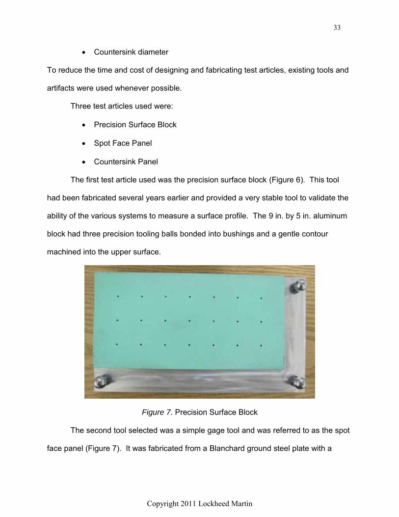
The first test article used was the precision surface block (Figure 6). This tool
had been fabricated several years earlier and provided a very stable tool to validate the
ability of the various systems to measure a surface profile. The 9 in. by 5 in. aluminum
block had three precision tooling balls bonded into bushings and a gentle contour
machined into the upper surface.
Figure 7. Precision Surface Block
The second tool selected was a simple gage tool and was referred to as the spot
face panel (Figure 7). It was fabricated from a Blanchard ground steel plate with a

34
Copyright 2011 Lockheed Martin
series of spot faces machined into the surface to represent fastener heads. The
purpose of the gage tool was to provide a simple tool with as little variation as possible
to assess accuracy and repeatability. Two thirds of the tool was coated with black oxide
and one third of the tool was painted with green aircraft primer to evaluate the effects of
shininess. A drawing of the gage tool can be found in Appendix A.
Figure 8. Spot Face Panel
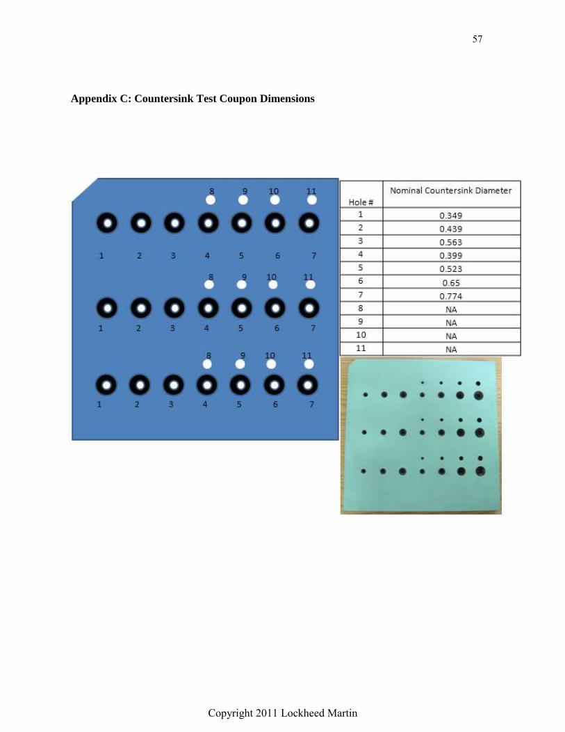
The last artifact, known as the countersink panel, was created from a 12 in.
square graphite-epoxy test panel. The test panel was .500 in. thick and had twenty-one
countersinks drilled into the surface and twelve non-countersunk holes. The
countersinks ranged from .350 in. to .750 in. in diameter. The panel was painted with
green aircraft primer, and the countersinks were machined after the primer was applied
so the resulting countersinks were black. This tool was originally fabricated to ascertain
the ability of white light systems to determine the depth and diameter of countersinks,

35
Copyright 2011 Lockheed Martin
the diameter of drilled holes, and locations of both holes and countersinks, however,
due to time limitations only countersink diameters were evaluated. A drawing of the
panel is included in Appendix B.
Figure 9. Countersink Panel
Benchmarking
Each test article was built in accordance to a design model, but since the study
was not concerned with the capability of the machines producing the test articles, the
only values of concern were the as-built nominal values. Once the features were
measured by the contact measurement methods these were the values by which all
other analysis would be compared to. In order to evaluate the performance of the non-
contact systems it was critical to have reliable nominal values of the features and test
articles.
The first test artifact was the precision surface block. A computer model was
provided to the CMM programmer and an inspection routine was developed. Once the
CMM program was transferred to the CMM controller, the test article was inspected.

36
Copyright 2011 Lockheed Martin
.
The surface and spot faces of the spot face panel were inspected with a Fowler
digital indicator (Model 54-520-777) attached to a height gage. The indicator was
zeroed on the top of the surface plate and then measurements were recorded in four
locations. These four measurement values were averaged to become the nominal spot
face depth.
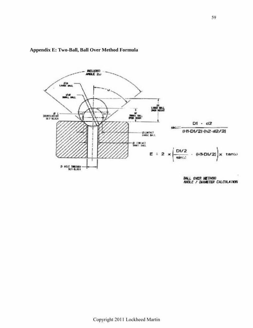
To baseline the countersink panel a two-ball, ball over method was used to
measure the countersink diameter of the countersink at the surface. Using this method,
two spheres were placed one at a time in the countersink. With the sphere in the
countersink, the height of the sphere relative to the top of the countersink was recorded.
This process is repeated for the second sphere. Using the formula in Appendix F the
diameter of each countersink was calculated.
Non-Contact Data Collection
The collection of the non-contact measurement data took place over a course of
a two week period with one system tested the first week and two systems tested the
following week. The vendors shipped their equipment to the Lockheed facility on the
Friday before testing which meant Monday morning was spent unpacking and
calibrating the equipment. Measurements started Monday afternoon and continued
through Friday morning allowing for time to pack up the equipment and ready it for
shipment.
Measurement data from white light systems is captured by cameras and
triangulated by software, and therefore limited by the field of view of the camera at a
given focal length. To overcome this limitation, some systems utilized photogrammetry
37
Copyright 2011 Lockheed Martin
to map the artifacts and provide a scaled reference frame. Each vendor utilized their
own photogrammetry equipment.
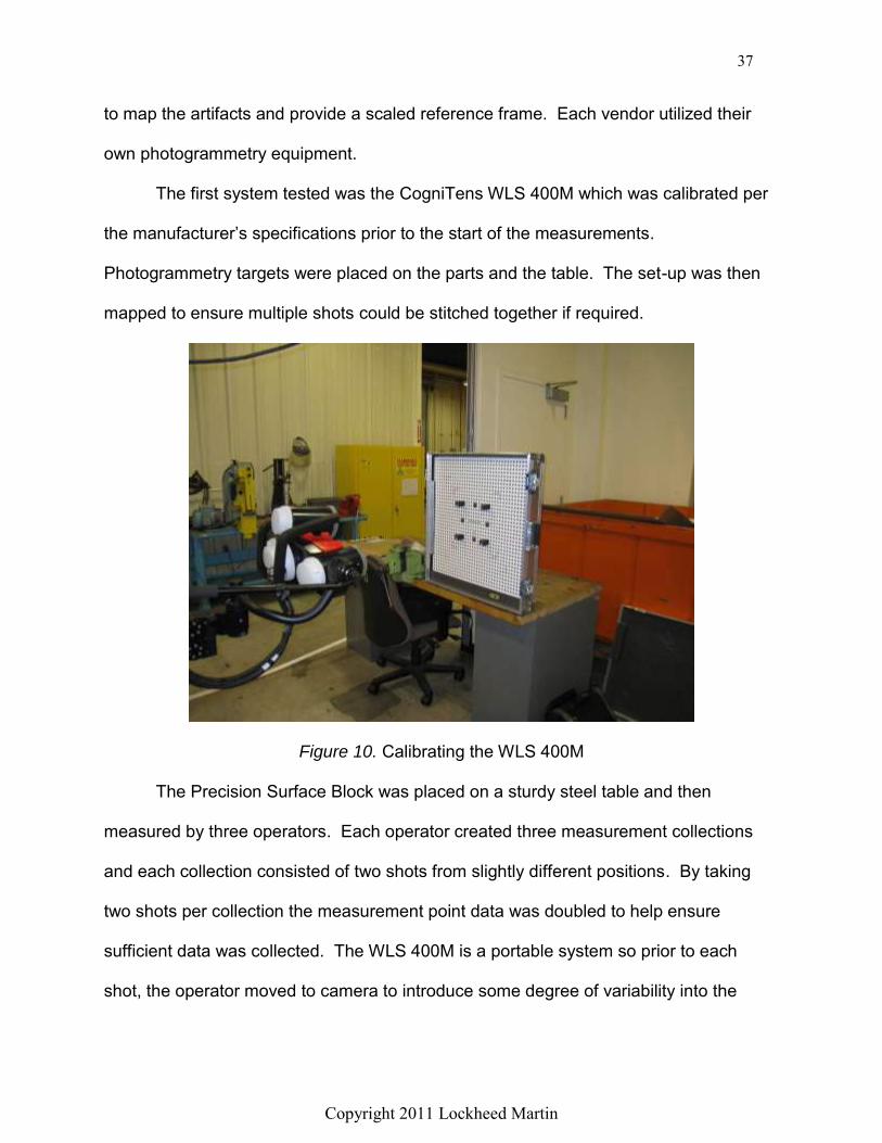
The first system tested was the CogniTens WLS 400M which was calibrated per
the manufacturer’s specifications prior to the start of the measurements.
Photogrammetry targets were placed on the parts and the table. The set-up was then
mapped to ensure multiple shots could be stitched together if required.
Figure 10. Calibrating the WLS 400M
The Precision Surface Block was placed on a sturdy steel table and then
measured by three operators. Each operator created three measurement collections
and each collection consisted of two shots from slightly different positions. By taking
two shots per collection the measurement point data was doubled to help ensure
sufficient data was collected. The WLS 400M is a portable system so prior to each
shot, the operator moved to camera to introduce some degree of variability into the

38
Copyright 2011 Lockheed Martin
process. The actual acquisition of the measurement is taken by pointing the camera at
the part and pressing a button, so variation form the operators should be minimal.
Figure 11. Measuring the Precision Surface Block with the WLS 400M
The Spot Face Panel was the next artifact measured. This artifact was
measured in the same manner as the Precision Surface Block; three operators, each
taking three collections. As before, each collection consisted of two shots to ensure
adequate point density.
Figure 12. Measuring the Spot Face Panel with the WLS 400M

39
Copyright 2011 Lockheed Martin
The last artifact to be measured was the countersink panel. Countersinks pose a
big challenge to non-contact systems. Without sufficient point data, the measurement
system may not actually collect a data point at the intersection of the edge of the
surface and the start of the countersink. Accurately measuring features such as
countersinks may require additional post processing software such as PolyWorks or
Geomagic. These software programs are better suited to best-fit a cone or similar
feature into the data for comparative purposes. While countersink measurement can be
a difficult task, it is one that aerospace manufacturers would benefit greatly from.
Figure 13. Measuring the Countersink Panel with the WLS 400M
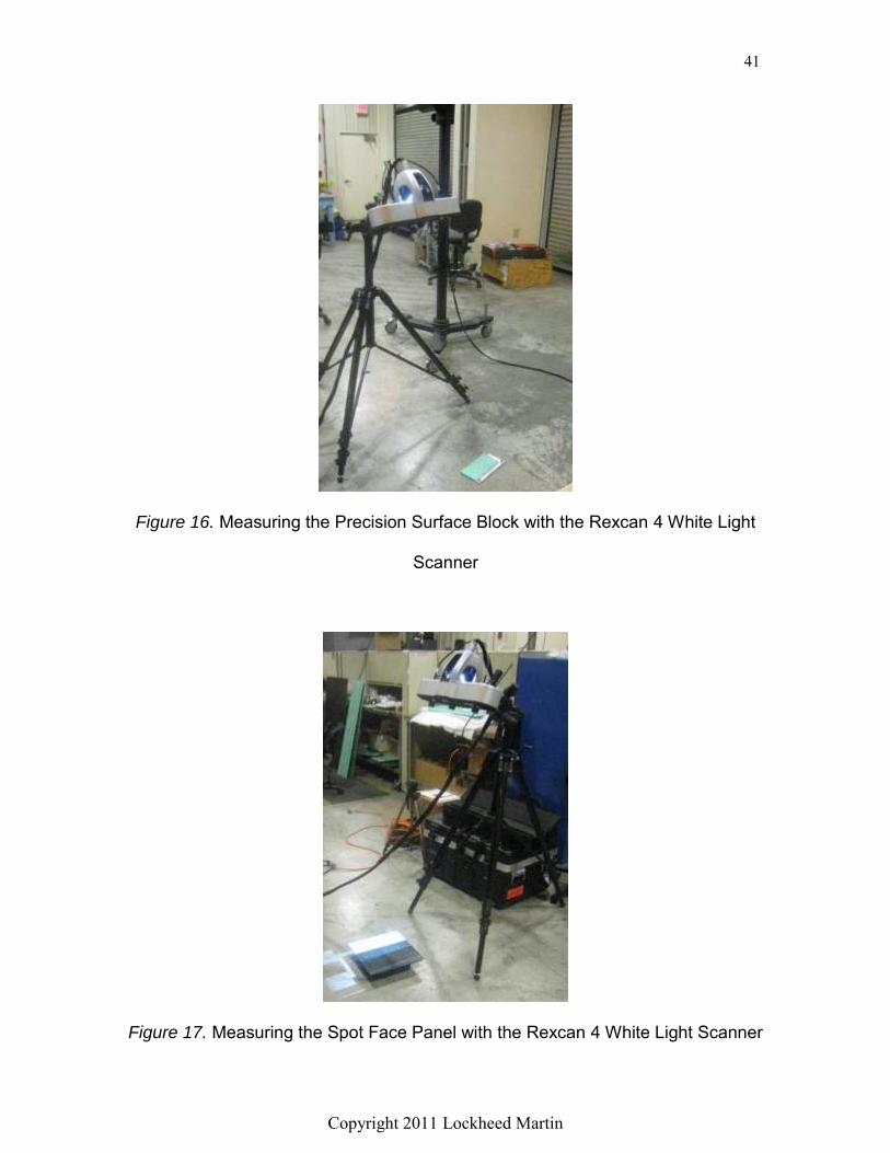
During the second week of testing two systems were evaluated. The Rexcan 4
by Solutionix and the ATOS Triple Scan by GOM were both evaluated using the same

40
Copyright 2011 Lockheed Martin
procedures as the previous two systems. For these two systems photogrammetric
mapping was used to stitch multiple images together. Once the parts were mapped, the
data acquisition followed with the Precision Surface Block first, the Spot Face Panel
second and the Countersink Panel last.
Figure 14. Calibrating the Rexcan 4 White Light Scanner
Figure 15. Mapping the Artifact with Photogrammetry
41
Copyright 2011 Lockheed Martin
Figure 16. Measuring the Precision Surface Block with the Rexcan 4 White Light
Scanner
Figure 17. Measuring the Spot Face Panel with the Rexcan 4 White Light Scanner

42
Copyright 2011 Lockheed Martin
Figure 18. Measuring the Countersink Panel with the Rexcan 4 White Light Scanner
Figure 19. Measuring the Precision Surface Block with the ATOS Triple Scan

43
Copyright 2011 Lockheed Martin
Figure 20. Measuring the Spot Face Panel with the ATOS Triple Scan
Figure 21. Measuring the Countersink Panel with the ATOS Triple Scan

44
Copyright 2011 Lockheed Martin
Gage Repeatability and Reproducibility Study
A gage repeatability and reproducibility (gage R&R) study should always be
performed for new inspection processes. The gage R&R is used to determine if the
measurement system is capable of providing correct inspection data for the tolerances
specified. As noted in the literature review, there is no single specification to guide the
gage R&R study. For this study three operators were selected to collect the data with
the non-contact systems. Each operator measured each test article three times,
capturing twenty-one features or measurement points. A matrix of the data collection
forms can be found in the Appendix of this report. Once the data was collected, Minitab
16.2.0.0 software was used to analyze the data using the ANOVA method. The output
from Minitab provided information on the range of the measurement variation, the
standard deviation of the results and a precision to tolerance ratio that indicates how
capable the measurement system is for the intended use. Linearity and bias data were
also provided.

45
Copyright 2011 Lockheed Martin
Chapter IV: Results
Non-contact methods of inspection have been developed over the last fifteen
years, but there is limited data comparing the accuracy of these technologies to contact
methods of inspection. This study was conducted to make such a comparison.
Results
The analysis of this study was conducted using Minitab 16.2.0.0 software and is
contained in the appendix of this paper.
Summary of Findings
Three non-contact metrology systems were used to measure three distinct test
artifacts.
Non-contact Metrology Systems:
1. CogniTens WLS 400M White Light Scanner
2. ATOS Triple Scan With Blue Light Technology
3. Rexcan 4 White Light Scanner
Test Artifacts:
1. Precision Surface Plate
2. Spot Face Panel
3. Countersink Panel
The Precision Surface Plate evaluated the ability of each system to measure a
contoured surface and relate the points back to a nominal solid model. The Spot Face
Panel simulated measuring installed fastener depths, and the Countersink Panel tested
the ability to measure the diameter of a countersink. The Gage R&R was performed

46
Copyright 2011 Lockheed Martin
utilizing the tolerances in Table 1 which are listed in inches. The full gage study results
are provided in the appendix of this paper.
Table 1: Test Article Tolerances Test Article Lower Tolerance Upper Tolerance
Precision Surface Block -.005” .005”
Spot Face Panel .000” .020”
Countersink Panel -.010” .010”
Gage Linearity and Bias Study
Gage linearity and bias are measurements of how accurate the measurement
system is relative to the baseline or reference value and how accurate it is across the
full range of intended measurements. Bias indicates the accuracy and linearity tells
how consistent the system is. The following table presents the bias of each system
relative to the nominal values. If the bias is higher than zero the system overestimates
the measurement and if the bias is negative it underestimates the measurement
(Minitab, 2007).
Table 2: Average Bias of Each Measurement System Test Article CogniTens WLS
400M ATOS Triple
Scan Rexcan 4 White
Light System Precision Surface Block -0.00010” 0.00015” 0.00028”
Spot Face Panel 0.00009” -0.00010” 0.00087”
Countersink Panel 0.00285” -0.00032” 0.00166”
Gage linearity describes how accurate the measurement system is across the
range of measurement process. Linearity is expressed as the slope of the
measurement bias as well as a %Linearity, which is linearity expressed as a percent of

47
Copyright 2011 Lockheed Martin
the process variation (Minitab, 2007). Linearity data is provided in Table 3. Small
linearity values indicate the accuracy remains the same throughout the measurement
range.
Table 3: Linearity Values for Each System Measuring and Each Test Article Test Article CogniTens WLS
400M ATOS Triple
Scan Rexcan 4 White
Light System Precision Surface Block 0.00120 0.00175
0.00051
Spot Face Panel 0.00029 0.00056 0.00482
Countersink Panel 0.02110 0.01197
0.00140
%Linearity provides a metric to show measurement consistency. The closer %Linearity
is to zero, the more consistently the gage measures across the measurement range
(Minitab, 2007). Table 4 provides %Linearity data.
Table 4: %Linearity Values for Each System Measuring and Each Test Article Test Article CogniTens WLS
400M ATOS Triple
Scan Rexcan 4 White
Light System Precision Surface Block 2.20%
3.10%
0.90%
Spot Face Panel 0.07%
1.30%
12.10%
Countersink Panel 2.50%
1.50%
0.20%
Gage Repeatability and Reproducibility Study
A gage R&R study is useful to determine the amount of variation in a
measurement device or system as well as the source of the variation. Measurement
repeatability measures the variation between measurements taken by a single operator
and should be low. Table 5 provides the measurement repeatability for the systems.

48
Copyright 2011 Lockheed Martin
Table 5: Gage R&R Repeatability Results Test Article CogniTens WLS
400M ATOS Triple
Scan Rexcan 4 White
Light System Precision Surface Block 0.06%
0.01%
0.92%
Spot Face Panel 0.52%
0.21%
18.57%
Countersink Panel 0.02%
0.01%
0.09%
Gage Reproducibility measures the amount of variation between operators
measuring the same part. Table 6 provides reproducibility data.
Table 6: Gage R&R Reproducibility Results Test Article CogniTens WLS
400M ATOS Triple
Scan Rexcan 4 White
Light System Precision Surface Block 0.02%
0.00%
0.12%
Spot Face Panel 0.05%
0.10%
1.21%
Countersink Panel 0.00%
0.03%
0.01%
Typically, the total gage variation for a measurement system would equal less
than 30% of the tolerance while less than 10% would be preferred (Minitab, 2007).
Table 7 provides the total gage variation as a percent of the tolerance.
Table 7: Total Gage R&R Variation as A Percent of the Tolerance
Test Article CogniTens WLS 400M
ATOS Triple Scan
Rexcan 4 White Light System
Precision Surface Block 15.18%
5.94%
55.40%
Spot Face Panel 15.33%
11.45%
88.88%
Countersink Panel 64.58%
80.30%
179%

49
Copyright 2011 Lockheed Martin
Table 8 provides a breakdown of measurement system acceptability based on a 30%
variation/tolerance ratio.
Table 8: Acceptability of the Measurement Systems Based On 30% Variation/Tolerance Ratio Test Article CogniTens WLS
400M ATOS Triple
Scan Rexcan 4 White
Light System Precision Surface Block Acceptable
Acceptable
Unacceptable
Spot Face Panel Acceptable
Acceptable
Unacceptable
Countersink Panel Unacceptable
Unacceptable
Unacceptable
50
Copyright 2011 Lockheed Martin
Chapter V: Discussion
Non-contact metrology devices have made tremendous advances in the last ten
years and offer potential solutions to manufacturing challenges. Allowing quick
inspection of complex parts earlier in the manufacturing process offers the opportunity
to reduce scrap and increase part quality. Before any new inspection technology can
be utilized in an inspection process the system must be qualified for that given process.
This study evaluated the ability of three white light measurement systems to measure
surface contour, spot face depth (simulating fasters in a structure) and countersinks.
Conclusions
The results of this study show that the CogniTens WLS 400M and the GOM
ATOS Triple Scan are capable of accurately and repeatedly measuring surface profiles
and spot faces within the tested measurement tolerance range. However, neither
system was capable of measuring countersink diameters using point cloud data for
analysis. The Rexcan 4 White Light Scanner was not capable of achieving reliable
results for any of the measured test article.
Recommendations
The Rexcan 4 White Light Scanner was included in this study because it costs
significantly less than either the CogniTens or the ATOS scanners. Testing it against
the tight tolerances in this study showed it is not a capable instrument for this purpose.
However, given a wider tolerance band and different application, the Rexcan 4 may
show to be a cost effective alternative.

51
Copyright 2011 Lockheed Martin
The CogniTens WLS 400M and GOM ATOS Triple Scan both proved to be
capable systems but each system has strengths and weakness that also need to be
considered for each application. While the ATOS system has slightly better results, the
ATOS system is sensitive to vibration and cannot be hand held. Since the CogniTens
WLS 400M acquires measurement data in milliseconds it can be hand held and can be
used in a wider range of production-type environments. In addition, the CogniTens
WLS 400M has a Vision Mode feature that allows the scanner to look for contrast
details on the surface. Countersink measurement data using this feature wasn’t
included in this study since the other two systems do not have it, but using the vision
mode offered much improved measurement data on the painted countersink panel.
However, if the panel had not been painted and there was not significant color contrast
between the countersink and the surface, it is not clear the vision mode advantage
would be maintained.
Collecting measurement data is relatively easy but knowing how to analyze takes
effort. While the ATOS and CogniTens systems were demonstrated to be capable,
there is certainly a need for improved algorithms to speed up the analysis of the data.
Now that the equipment has been shown to be capable, a follow-on study should be
conducted to analyze the measurement process to achieve optimized results.
52
Copyright 2011 Lockheed Martin
References
3D surface reconstruction technologies. (2008). North Kingstown, R.I.: Hexagon Metrology.
Basics of the cmm 120: Inspection training. (2011). Retrieved from
http://www.toolingu.com/definition-350120-22452-coordinate-measuring-machine.html.
Benchmark. (n.d.). In The free dictionary by farlex. Retrieved from
http://www.thefreedictionary.com/benchmark.
Boucher, M. (2007, July). Using offline programming keeps that cmm on track. Tooling and
Production. 73. (7). 32-33.
Bucher, J.L. (Ed.). (2004). The metrology handbook. Milwaukee, WI, ASQ Quality Press.
Card, G. (2003, June) Selecting your cmm. Manufacturing Engineering, 130, (6) 71-76, 78.
Chapman, W. (Ed.). (2002). Modern machine shop: Handbook for the metalworking industries.
Cincinnati, OH. Hanser Gardner Publications.
Goldsmith, M. (2010). Good practice guide no. 118: A beginner’s guide to measurement. United
Kingdom, Queen’s Printer and Controller of HMSO.
Hammett, P.C. & Garcia Guzman, L. (2006). White light measurement: A catalyst for change in
automotive body dimensional validation: Measurement strategies for stamping and body
assembly from tryout through PPAP. (UMTRI-2006-3). Ann Arbor, Michigan.
Hammett, P.C., Guzman, LG., Frescoln K.D. & Ellison, S.J. (2005). Proceedings from SAE
World Congress. Changing automotive body measurement system paradigms with 3D
non-contact measuring systems. Warrendale, PA: SAE International.
Kalpakjian, S. (1992). Manufacturing engineering and technology. (2nd ed.). Reading,
Massachusetts, Addison-Wesley Publishing Company.

53
Copyright 2011 Lockheed Martin
Kappele, W.D. & Raffaldi, J.D. (2005, December). An introduction to gage r&r. Quality, 44
(13), 24-25.
Kinard, D. (2010, September). The digital thread - Key to F-35 joint strike fighter affordability.
Aerospace Manufacturing and Design. Retrieved from
http://www.onlineamd.com/Author.aspx?AuthorID=5187
Logee, S., Fabiano, R., & Cassola, J. (2009). Little CMM that could. Tool and Production, 75,
(5/6), 32-33.
Metrology. (n.d.). In The free dictionary by farlex. Retrieved from
http://www.thefreedictionary.com/metrology.
Micron. (n.d.). In The free dictionary by farlex. Retrieved from
http://www.thefreedictionary.com/micron.
Minitab Inc. (2007). Minitab Statistical Software, Release 15 for Windows, State College,
Author, PA.
Minitab Inc. (2010). Gage studies for continuous data, Release 16, Version 1.0, State College,
Author, PA. Retrieved from
http://www.minitab.com/uploadedFiles/Shared_Resources/Documents/Sample_Materials
/TrainingSampleMeasurementSystemsMTB16EN.pdf
Morey, B. (2009, November). Shop floor metrology. Manufacturing Engineering, 143, (5), 55-
60.
Morey, B. (2010a, July). Metrology with white light. Manufacturing Engineering, 145, (1), 55-
61.
Morey, B. (2010b, September). Advances in automotive metrology. Manufacturing Engineering,
145, (3), 53-61.
54
Copyright 2011 Lockheed Martin
Morey, B. (2010c, November). Accuracy and uncertainty in non-contact metrology.
Manufacturing Engineering, 145, (5), 67-74.
Morey, B. (2011, March). Aerospace metrology tools for the working day. Manufacturing
Engineering, 143, (3), 53-65.
Mraz, S.J. (2011, July). Cmm gets easier to use. Machine Design, 83, (12), 18.
Nikon Laser Radar Training Workbook (2010). Brighton, MI.: Nikon Metrology.
O’Rourke. K. (2011, April). Strength in numbers. Quality, 50, (4), 36-38.
Roe, J.W. (1916). English and American tool builders, Yale University Press.
Sloop, R. (2009, September). Understand gage r&r. Quality, 48, (9) 44-47.
Starrett (2011a). General micrometer information. Retrieved from
http://www.starrett.com/download/222_p1_5.pdf
Starrett (2011b). Slide Calipers. Retrieved from
http://www.starrett.com/download/246_p108_114.pdf

55
Copyright 2011 Lockheed Martin
Appendix A: Spot Face Panel Drawing
.: ---------!

56
Copyright 2011 Lockheed Martin
Appendix B: Spot Face Panel Benchmark Results
Dia. (Column) A - Depth B - Depth C - Depth D - Depth Averaged Nominal 0.375” (1) 0.0006” 0.0006” 0.0007” 0.0006” 0.0006 0.375” (2) 0.0011” 0.0012” 0.0011” 0.0011” 0.0011 0.375” (3) 0.0038” 0.0039” 0.0037” 0.0034” 0.0037 0.375” (4) 0.0075” 0.0079” 0.0080” 0.0073” 0.0077 0.375” (5) 0.0113” 0.0118” 0.0118” 0.0112” 0.0115 0.375” (6) 0.0152” 0.0154” 0.0156” 0.0156” 0.0155 0.375” (7) 0.0192” 0.0193” 0.0197” 0.0195” 0.0194
0.500” (1) 0.0009” 0.0009” 0.0010” 0.0007” 0.0009 0.500” (2) 0.0014” 0.0016” 0.0018” 0.0015” 0.0016 0.500” (3) 0.0032” 0.0038” 0.0039” 0.0032” 0.0035 0.500” (4) 0.0073” 0.0080” 0.0080” 0.0070” 0.0076 0.500” (5) 0.0105” 0.0107” 0.0109” 0.0108” 0.0107 0.500” (6) 0.0156” 0.0154” 0.0156” 0.0159” 0.0156 0.500” (7) 0.0193” 0.0193” 0.0196” 0.0194” 0.0194
0.625” (1) 0.0013” 0.0016” 0.0015” 0.0012” 0.0014 0.625” (2) 0.0018” 0.0019” 0.0022” 0.0018” 0.0019 0.625” (3) 0.0031” 0.0043” 0.0032” 0.0031” 0.0034 0.625” (4) 0.0077” 0.0078” 0.0073” 0.0072” 0.0075 0.625” (5) 0.0122” 0.0120” 0.0115” 0.0115” 0.0118 0.625” (6) 0.0161” 0.0152” 0.0154” 0.0164” 0.0158 0.625” (7) 0.0195” 0.0184” 0.0187” 0.0194” 0.0190
57
Copyright 2011 Lockheed Martin
Appendix C: Countersink Test Coupon Dimensions

58
Copyright 2011 Lockheed Martin
Appendix D: Precision Surface Block
59
Copyright 2011 Lockheed Martin
Appendix E: Two-Ball, Ball Over Method Formula
0 1 . d2
p,w: (H)-01/2 H I\2 ·d2/2l
1 0112 e: : 2 )( \ sin<J.: I) tanw • IH)-0112 X

60
Copyright 2011 Lockheed Martin
Appendix F: Input Data and Results for Precision Surface Panel
CogniTens WLS 400M Input Data
Operator 1 Operator 2 Operator 3
Nominal Rep 1 Rep 2 Rep 3 Rep 1 Rep 2 Rep 3 Rep 1 Rep 2 Rep 3
0.1024 0.10419 0.10412 0.10415 0.10395 0.10389 0.10386 0.1041 0.10385 0.10371
0.0952 0.09654 0.09649 0.09658 0.09666 0.09617 0.09645 0.09658 0.09637 0.09621
0.0933 0.09437 0.09436 0.0944 0.09433 0.09403 0.09414 0.09458 0.09429 0.0942
0.0930 0.0938 0.09385 0.09395 0.09369 0.09366 0.09352 0.0939 0.09383 0.09421
0.0928 0.09342 0.09313 0.09344 0.09339 0.09305 0.09317 0.09335 0.09311 0.09421
0.0929 0.09285 0.09279 0.09299 0.09295 0.09246 0.09267 0.09296 0.09276 0.09371
0.0950 0.09444 0.09432 0.09453 0.09451 0.09407 0.09414 0.09466 0.09435 0.09491
0.0946 0.09544 0.09543 0.0955 0.09551 0.09532 0.09535 0.09555 0.09531 0.09512
0.0997 0.09995 0.10006 0.10005 0.10002 0.09977 0.0999 0.10012 0.09985 0.09974
0.1027 0.1027 0.10281 0.10282 0.10268 0.10249 0.10255 0.10311 0.10277 0.10297
0.1020 0.10195 0.10182 0.10202 0.10194 0.10168 0.10156 0.10218 0.10188 0.10283
0.0976 0.09691 0.09671 0.09698 0.0971 0.09658 0.09676 0.09706 0.09676 0.09775
0.0897 0.08896 0.0889 0.08908 0.08916 0.08865 0.0888 0.08927 0.08901 0.08927
0.0821 0.08098 0.08091 0.08117 0.0812 0.08068 0.08073 0.08132 0.08094 0.08106
0.1012 0.10141 0.10145 0.10149 0.10149 0.10133 0.10129 0.10158 0.10127 0.10113
0.1093 0.10884 0.1089 0.10891 0.109 0.10873 0.10891 0.10921 0.10885 0.1088
0.1120 0.11111 0.11121 0.11127 0.11126 0.11104 0.11104 0.11168 0.11127 0.11176
0.1080 0.10679 0.10691 0.10701 0.10708 0.10684 0.10665 0.10726 0.10692 0.10801
0.0977 0.09649 0.09653 0.09674 0.09687 0.09635 0.09653 0.0969 0.0966 0.097
0.0848 0.08329 0.08339 0.08352 0.08358 0.08324 0.08317 0.08384 0.08351 0.08347
0.0735 0.07225 0.07209 0.07243 0.07245 0.07195 0.0719 0.0727 0.07227 0.07232

61
Copyright 2011 Lockheed Martin
0.110.100.090.080.07
0.002
0.001
0.000
-0.001
-0.002
Reference Value
Bia
s
0
Regression
95% CI
Data
Avg Bias
BiasLinearity
2
1
0
Pe
rce
nt
C onstant -0.0022090 0.0006800 0.001
Slope 0.021889 0.007041 0.002
Predictor C oef SE C oef P
Gage Linearity
S 0.0008577 R-Sq 4.9%
Linearity 0.0012239 %Linearity 2.2
A v erage -0.0001040 0.2 0.000
0.0735 -0.0012378 2.2 0.000
0.0821 -0.0011011 2.0 0.000
0.0848 -0.0013544 2.4 0.000
0.0897 -0.0006889 1.2 0.000
0.0928 0.0005633 1.0 0.003
0.0929 0.0000044 0.0 0.975
0.093 0.0008233 1.5 0.000
Reference Bias %Bias P
Gage Bias
Gage name: C ogniTens WLS 400M
Date of study : Nov 2011
Reported by : M. Hestness
Tolerance: ±.005
Misc: Precision Surface Block
Percent of Process Variation
Gage Linearity and Bias Study for Measured
Part-to-PartReprodRepeatGage R&R
400
200
0
Perc
ent
% Contribution
% Study Var
% Tolerance
Point
9
Point
8
Point
7
Point
6
Point
5
Point
4
Poin t
3
Point 21
Point 20
Point
2
Point 19
Point 1 8
Point 17
Point 16
Point 15
P oin t
14
Point 13
Point 12
Point 11
Point 10
Point
1
Point
9
Point
8
P oint
7
Point
6
Point
5
Point
4
Point
3
P oin t
21
Point 20
Point
2
Point 19
Point 18
Point 1 7
Point 16
Point 15
Point 14
Point 1 3
Point 12
Point 11
Point 10
Poin t
1
Point
9
Point
8
Point
7
P oin t
6
Point
5
Point
4
Point
3
Point 21
P oin t
2 0
Point
2
Point 19
Point 18
P oint
17
Point 16
Point 15
Point 14
Point 13
Point 1 2
Point 11
Point 10
Point
1
0.0010
0.0005
0.0000
Points
Sam
ple
Range
_R=0.000359
UCL=0.000924
LCL=0
Operator 1 Operator 2 Operator 3
Point 9
Point 8
Point 7
Point 6
Point 5
Point 4
P oin t
3
Poin
t 21
Poin
t 20
Point 2
Po in
t 19
Poin
t 18
Poin
t 17
Poin
t 16
Poin
t 15
Poin
t 14
Poin
t 13
Poin
t 12
Poin
t 11
Po in
t 10
Point 1
Point 9
Point 8
P oint
7
Point 6
Point 5
Point 4
Point 3
Poin
t 21
Poin
t 20
Point 2
Poin
t 19
Po in
t 18
Poin
t 17
Poin
t 16
Poin
t 15
Poin
t 14
Poin
t 13
Poin
t 12
Poin
t 11
Poin
t 10
Point 1
Point 9
Point 8
Point 7
P oin t
6
Point 5
Point 4
Point 3
Poin
t 21
Poin
t 20
Point 2
Poin
t 19
Poin
t 18
Poin
t 17
Poin
t 16
Poin
t 15
Poin
t 14
Po in
t 13
Poin
t 12
Poin
t 11
Poin
t 10
Point 1
0.11
0.09
0.07
Points
Sam
ple
Mean
__X=0.09606UCL=0.09643LCL=0.09570
Operator 1 Operator 2 Operator 3
Point 9
Point 8
Poi n
t 7
Poi n
t 6
Point 5
Point 4
Point 3
Point 2
1
Poi n
t 20
Point 2
Point 1
9
Point 1
8
Point 1
7
Poi n
t 16
Poi nt 1
5
Point 1
4
Point 1
3
Point 1
2
Poi n
t 11
Poi nt 1
0
Point 1
0.11
0.09
0.07
Points
Operator 3Operator 2Operator 1
0.11
0.09
0.07
Operator
Point 9
Point 8
Point 7
P oin t 6
Point 5
Point 4
Point 3
Poin
t 21
Poin
t 20
Point 2
Poin
t 19
Po in
t 18
Poin
t 17
Poin
t 16
Poin
t 15
Poin
t 14
Poin
t 13
Poin
t 12
Poin
t 11
Poin
t 10
P oint
1
0.11
0.09
0.07
Points
Avera
ge Operator 1
Operator 2
Operator 3
Operator
Gage name: C ogniTens WLS 400M
Date of study : Nov 2011
Reported by : M. Hestness
Tolerance: ±.005
Misc: Precision Surface Block
Components of Variation
R Chart by Operator
Xbar Chart by Operator
Z Location by Points
Z Location by Operator
Points * Operator Interaction
Gage R&R (ANOVA) for Z Location
·a ; I:- I ;. :
•
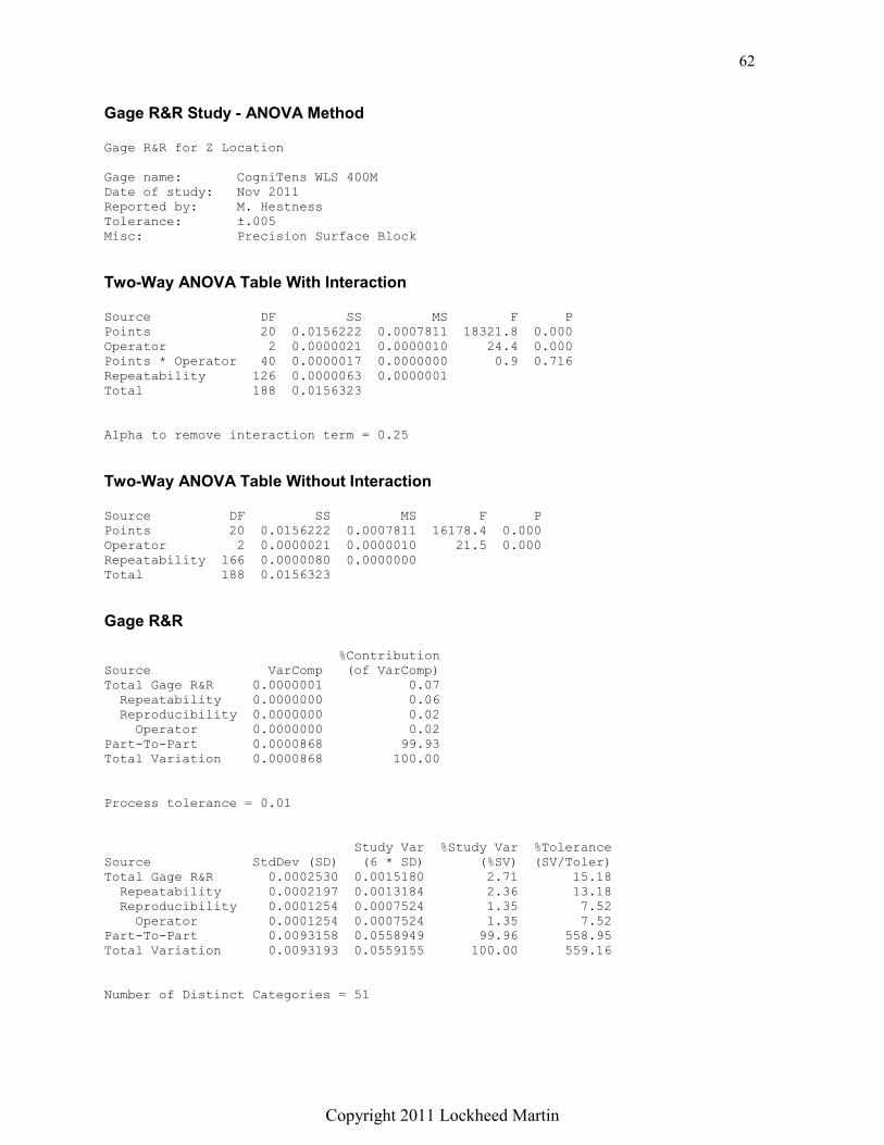
62
Copyright 2011 Lockheed Martin
Gage R&R Study - ANOVA Method Gage R&R for Z Location
Gage name: CogniTens WLS 400M
Date of study: Nov 2011
Reported by: M. Hestness
Tolerance: ±.005
Misc: Precision Surface Block
Two-Way ANOVA Table With Interaction Source DF SS MS F P
Points 20 0.0156222 0.0007811 18321.8 0.000
Operator 2 0.0000021 0.0000010 24.4 0.000
Points * Operator 40 0.0000017 0.0000000 0.9 0.716
Repeatability 126 0.0000063 0.0000001
Total 188 0.0156323
Alpha to remove interaction term = 0.25
Two-Way ANOVA Table Without Interaction Source DF SS MS F P
Points 20 0.0156222 0.0007811 16178.4 0.000
Operator 2 0.0000021 0.0000010 21.5 0.000
Repeatability 166 0.0000080 0.0000000
Total 188 0.0156323
Gage R&R %Contribution
Source VarComp (of VarComp)
Total Gage R&R 0.0000001 0.07
Repeatability 0.0000000 0.06
Reproducibility 0.0000000 0.02
Operator 0.0000000 0.02
Part-To-Part 0.0000868 99.93
Total Variation 0.0000868 100.00
Process tolerance = 0.01
Study Var %Study Var %Tolerance
Source StdDev (SD) (6 * SD) (%SV) (SV/Toler)
Total Gage R&R 0.0002530 0.0015180 2.71 15.18
Repeatability 0.0002197 0.0013184 2.36 13.18
Reproducibility 0.0001254 0.0007524 1.35 7.52
Operator 0.0001254 0.0007524 1.35 7.52
Part-To-Part 0.0093158 0.0558949 99.96 558.95
Total Variation 0.0093193 0.0559155 100.00 559.16
Number of Distinct Categories = 51
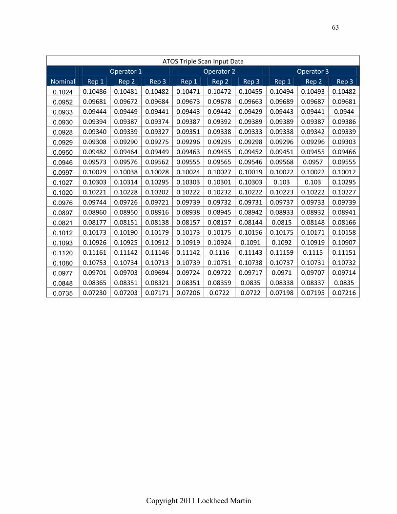
63
Copyright 2011 Lockheed Martin
ATOS Triple Scan Input Data
Operator 1 Operator 2 Operator 3
Nominal Rep 1 Rep 2 Rep 3 Rep 1 Rep 2 Rep 3 Rep 1 Rep 2 Rep 3
0.1024 0.10486 0.10481 0.10482 0.10471 0.10472 0.10455 0.10494 0.10493 0.10482
0.0952 0.09681 0.09672 0.09684 0.09673 0.09678 0.09663 0.09689 0.09687 0.09681
0.0933 0.09444 0.09449 0.09441 0.09443 0.09442 0.09429 0.09443 0.09441 0.0944
0.0930 0.09394 0.09387 0.09374 0.09387 0.09392 0.09389 0.09389 0.09387 0.09386
0.0928 0.09340 0.09339 0.09327 0.09351 0.09338 0.09333 0.09338 0.09342 0.09339
0.0929 0.09308 0.09290 0.09275 0.09296 0.09295 0.09298 0.09296 0.09296 0.09303
0.0950 0.09482 0.09464 0.09449 0.09463 0.09455 0.09452 0.09451 0.09455 0.09466
0.0946 0.09573 0.09576 0.09562 0.09555 0.09565 0.09546 0.09568 0.0957 0.09555
0.0997 0.10029 0.10038 0.10028 0.10024 0.10027 0.10019 0.10022 0.10022 0.10012
0.1027 0.10303 0.10314 0.10295 0.10303 0.10301 0.10303 0.103 0.103 0.10295
0.1020 0.10221 0.10228 0.10202 0.10222 0.10232 0.10222 0.10223 0.10222 0.10227
0.0976 0.09744 0.09726 0.09721 0.09739 0.09732 0.09731 0.09737 0.09733 0.09739
0.0897 0.08960 0.08950 0.08916 0.08938 0.08945 0.08942 0.08933 0.08932 0.08941
0.0821 0.08177 0.08151 0.08138 0.08157 0.08157 0.08144 0.0815 0.08148 0.08166
0.1012 0.10173 0.10190 0.10179 0.10173 0.10175 0.10156 0.10175 0.10171 0.10158
0.1093 0.10926 0.10925 0.10912 0.10919 0.10924 0.1091 0.1092 0.10919 0.10907
0.1120 0.11161 0.11142 0.11146 0.11142 0.1116 0.11143 0.11159 0.1115 0.11151
0.1080 0.10753 0.10734 0.10713 0.10739 0.10751 0.10738 0.10737 0.10731 0.10732
0.0977 0.09701 0.09703 0.09694 0.09724 0.09722 0.09717 0.0971 0.09707 0.09714
0.0848 0.08365 0.08351 0.08321 0.08351 0.08359 0.0835 0.08338 0.08337 0.0835
0.0735 0.07230 0.07203 0.07171 0.07206 0.0722 0.0722 0.07198 0.07195 0.07216
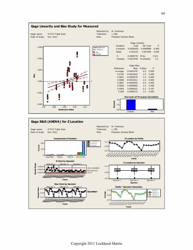
64
Copyright 2011 Lockheed Martin
0.110.100.090.080.07
0.003
0.002
0.001
0.000
-0.001
-0.002
Reference Value
Bia
s
0
Regression
95% CI
Data
Avg Bias
BiasLinearity
3.0
1.5
0.0
Pe
rce
nt
C onstant -0.0028433 0.0006958 0.000
Slope 0.031101 0.007205 0.000
Predictor C oef SE C oef P
Gage Linearity
S 0.0008776 R-Sq 9.1%
Linearity 0.0017549 %Linearity 3.1
A v erage 0.0001476 0.3 0.000
0.0735 -0.0014344 2.5 0.000
0.0821 -0.0005578 1.0 0.000
0.0848 -0.0013311 2.4 0.000
0.0897 -0.0003033 0.5 0.000
0.0928 0.0005856 1.0 0.000
0.0929 0.0000522 0.1 0.187
0.093 0.0008722 1.5 0.000
Reference Bias %Bias P
Gage Bias
Gage name: A TO S Triple Scan
Date of study : Nov 2011
Reported by : M. Hestness
Tolerance: ±.005
Misc: Precision Surface Block
Percent of Process Variation
Gage Linearity and Bias Study for Measured
Part-to-PartReprodRepeatGage R&R
500
250
0
Perc
ent
% Contribution
% Study Var
% Tolerance
Point
9
Poin t
8
Point
7
Point
6
P oint
5
Point
4
Point
3
Point 21
P oin t
20
Point
2
Point 19
Point 18
Point 17
Point 16
Point 15
P oin t
1 4
Point 13
Point 12
Point 11
Point 10
Point
1
Point
9
Point
8
Point
7
Point
6
Poin t
5
Point
4
Point
3
Point 21
Point 2 0
Point
2
Point 19
P oin t
18
Point 17
Point 16
Point 15
Point 14
Point 13
Point 12
P oin t
1 1
Point 10
Point
1
P oin t
9
Point
8
Point
7
Point
6
Point
5
Point
4
Point
3
P oint
21
Point 20
Point
2
Point 19
Point 1 8
Point 17
Point 16
P oin t
15
Point 14
Point 13
Point 12
Point 11
Point 10
Point
1
0.00050
0.00025
0.00000
Points
Sam
ple
Range
_R=0.0001510
UCL=0.0003886
LCL=0
Operator 1 Operator 2 Operator 3
Point 9
P oin t
8
Point 7
Point 6
Point 5
Point 4
Point 3
Poin
t 21
Poin
t 20
Point 2
Poin
t 19
Po in
t 18
Poin
t 17
Poin
t 16
Poin
t 15
Poin
t 14
Poin
t 13
Poin
t 12
Po in
t 11
Poin
t 10
Point 1
Point 9
Point 8
Point 7
Point 6
Point 5
Point 4
Point 3
Po in
t 21
Poin
t 20
Point 2
Poin
t 19
Poin
t 18
Poin
t 17
Poin
t 16
Po in
t 15
Poin
t 14
Poin
t 13
Poin
t 12
Poin
t 11
Poin
t 10
Point 1
P oin t
9
Point 8
Point 7
Point 6
Point 5
Point 4
Point 3
Poin
t 21
Poin
t 20
Point 2
Po in
t 19
Poin
t 18
Poin
t 17
Poin
t 16
Poin
t 15
Poin
t 14
Poin
t 13
Po in
t 12
Poin
t 11
Poin
t 10
Point 1
0.11
0.09
0.07
Points
Sam
ple
Mean
__X=0.09631UCL=0.09647LCL=0.09616
Operator 1 Operator 2 Operator 3
Point 9
Point 8
Poi n
t 7
Poi n
t 6
Point 5
Point 4
Point 3
Point 2
1
Poi n
t 20
Point 2
Point 1
9
Point 1
8
Point 1
7
Poi n
t 16
Poi nt 1
5
Point 1
4
Point 1
3
Point 1
2
Poi n
t 11
Poi nt 1
0
Point 1
0.11
0.09
0.07
Points
Operator 3Operator 2Operator 1
0.11
0.09
0.07
Operator
Point 9
Point 8
Point 7
P oin t 6
Point 5
Point 4
Point 3
Poin
t 21
Poin
t 20
Point 2
Poin
t 19
Po in
t 18
Poin
t 17
Poin
t 16
Poin
t 15
Poin
t 14
Poin
t 13
Poin
t 12
Poin
t 11
Poin
t 10
P oint
1
0.11
0.09
0.07
Points
Avera
ge Operator 1
Operator 2
Operator 3
Operator
Gage name: A TO S Triple Scan
Date of study : Nov 2011
Reported by : M. Hestness
Tolerance: ±.005
Misc: Precision Surface Block
Components of Variation
R Chart by Operator
Xbar Chart by Operator
Z Location by Points
Z Location by Operator
Points * Operator Interaction
Gage R&R (ANOVA) for Z Location
I •
1 . J l l~ I . . _ EZ:SL:::::I I
~I
I! ! !I tv\r-1D

65
Copyright 2011 Lockheed Martin
Gage R&R Study - ANOVA Method Gage R&R for Z Location
Gage name: ATOS Triple Scan
Date of study: Nov 2011
Reported by: M. Hestness
Tolerance: ±.005
Misc: Precision Surface Block
Two-Way ANOVA Table With Interaction Source DF SS MS F P
Points 20 0.0159177 0.0007959 73536.4 0.000
Operator 2 0.0000000 0.0000000 0.0 0.975
Points * Operator 40 0.0000004 0.0000000 1.1 0.285
Repeatability 126 0.0000012 0.0000000
Total 188 0.0159193
Alpha to remove interaction term = 0.25
Two-Way ANOVA Table Without Interaction Source DF SS MS F P
Points 20 0.0159177 0.0007959 81253.4 0.000
Operator 2 0.0000000 0.0000000 0.0 0.973
Repeatability 166 0.0000016 0.0000000
Total 188 0.0159193
Gage R&R %Contribution
Source VarComp (of VarComp)
Total Gage R&R 0.0000000 0.01
Repeatability 0.0000000 0.01
Reproducibility 0.0000000 0.00
Operator 0.0000000 0.00
Part-To-Part 0.0000884 99.99
Total Variation 0.0000884 100.00
Process tolerance = 0.01
Study Var %Study Var %Tolerance
Source StdDev (SD) (6 * SD) (%SV) (SV/Toler)
Total Gage R&R 0.0000990 0.0005938 1.05 5.94
Repeatability 0.0000990 0.0005938 1.05 5.94
Reproducibility 0.0000000 0.0000000 0.00 0.00
Operator 0.0000000 0.0000000 0.00 0.00
Part-To-Part 0.0094038 0.0564226 99.99 564.23
Total Variation 0.0094043 0.0564257 100.00 564.26
Number of Distinct Categories = 133

66
Copyright 2011 Lockheed Martin
Rexcan 4 White Light Scanner Input Data
Operator 1 Operator 2 Operator 3
Nominal Rep 1 Rep 2 Rep 3 Rep 1 Rep 2 Rep 3 Rep 1 Rep 2 Rep 3
0.1024 0.10584 0.10367 0.10459 0.10485 0.10523 0.10419 0.10461 0.10473 0.10504
0.0952 0.09663 0.09694 0.0957 0.09679 0.09697 0.09635 0.09535 0.09567 0.09546
0.0933 0.09531 0.09493 0.09314 0.09474 0.09439 0.09534 0.09414 0.0944 0.09318
0.0930 0.09549 0.09431 0.09455 0.09374 0.09438 0.09617 0.09386 0.09339 0.09374
0.0928 0.09311 0.09258 0.09343 0.09383 0.09466 0.09366 0.09304 0.09307 0.09422
0.0929 0.09319 0.09289 0.09265 0.09329 0.09269 0.09376 0.09334 0.09243 0.09315
0.0950 0.09521 0.09758 0.09715 0.0959 0.09611 0.09657 0.09472 0.09536 0.09609
0.0946 0.09587 0.09723 0.09543 0.09589 0.09725 0.09646 0.09624 0.09498 0.09728
0.0997 0.10198 0.10023 0.10052 0.10058 0.10029 0.09976 0.09906 0.09887 0.09936
0.1027 0.10306 0.10484 0.1035 0.10253 0.10265 0.1026 0.10367 0.1053 0.10415
0.1020 0.10241 0.10090 0.10032 0.10135 0.10157 0.10012 0.10287 0.10077 0.10187
0.0976 0.09689 0.09814 0.0971 0.09821 0.0964 0.09579 0.09683 0.09798 0.09836
0.0897 0.09109 0.09091 0.08946 0.09147 0.09005 0.08938 0.08861 0.09004 0.09077
0.0821 0.08236 0.08092 0.08083 0.08406 0.08156 0.08365 0.08161 0.08111 0.08221
0.1012 0.10287 0.10142 0.10263 0.10017 0.09902 0.10204 0.09981 0.10064 0.1019
0.1093 0.10935 0.10780 0.10888 0.10914 0.10938 0.10751 0.10932 0.1091 0.10974
0.1120 0.11077 0.11071 0.11262 0.11064 0.1088 0.10918 0.11137 0.11036 0.11182
0.1080 0.10782 0.10659 0.10819 0.10719 0.10603 0.10666 0.10739 0.10715 0.10651
0.0977 0.09702 0.09778 0.09778 0.09802 0.09783 0.09648 0.09827 0.09701 0.09747
0.0848 0.08364 0.08287 0.08398 0.08486 0.08354 0.0832 0.08343 0.08353 0.08472
0.0735 0.07260 0.07343 0.07298 0.07628 0.07159 0.07136 0.07306 0.07237 0.07391

67
Copyright 2011 Lockheed Martin
0.110.100.090.080.07
0.003
0.002
0.001
0.000
-0.001
-0.002
-0.003
-0.004
Reference Value
Bia
s 0
Regression
95% CI
Data
Avg Bias
BiasLinearity
1.0
0.5
0.0
Pe
rce
nt
C onstant 0.001189 0.001009 0.240
Slope -0.00945 0.01045 0.367
Predictor C oef SE C oef P
Gage Linearity
S 0.0012727 R-Sq 0.4%
Linearity 0.0005149 %Linearity 0.9
A v erage 0.0002808 0.5 0.000
0.0735 -0.0004356 0.8 0.441
0.0821 -0.0000656 0.1 0.857
0.0848 -0.0010478 1.9 0.002
0.0897 0.0004978 0.9 0.152
0.0928 0.0007111 1.3 0.016
0.0929 0.0001433 0.3 0.353
0.093 0.0014033 2.6 0.002
Reference Bias %Bias P
Gage Bias
Gage name: Rexcan 4 White Light Scanner
Date of study : Nov 2011
Reported by : M. Hestness
Tolerance: ±.005
Misc: Precision Surface Block
Percent of Process Variation
Gage Linearity and Bias Study for Measured
Part-to-PartReprodRepeatGage R&R
400
200
0
Perc
ent
% Contribution
% Study Var
% Tolerance
Point
9
Point
8
Point
7
Poin t
6
Point
5
Point
4
Point
3
Point 21
Point 20
Poin t
2
Point 1 9
Point 18
Point 17
Point 16
Point 15
P oint
14
Point 1 3
Point 12
Point 11
Point 10
Point
1
Poin t
9
Point
8
Point
7
Point
6
Point
5
Point
4
Poin t
3
Point 2 1
Point 20
Point
2
Point 19
Point 18
P oint
17
Point 1 6
Point 15
Point 14
Point 13
Point 12
P oint
11
Point 1 0
Point
1
Point
9
Point
8
Point
7
Poin t
6
Point
5
Point
4
Point
3
Point 21
Point 20
Poin t
2
Point 1 9
Point 18
Point 17
Point 16
Point 15
P oint
14
Point 1 3
Point 12
Point 11
Point 10
Point
1
0.004
0.002
0.000
Points
Sam
ple
Range
_R=0.001468
UCL=0.003779
LCL=0
Operator 1 Operator 2 Operator 3
Point 9
Point 8
Point 7
Point 6
Point 5
Point 4
Point 3
Poin
t 21
Poin
t 20
Point 2
Poin
t 19
Poin
t 18
Poin
t 17
Poin
t 16
Poin
t 15
Poin
t 14
Poin
t 13
Poin
t 12
Poin
t 11
Poin
t 10
Point 1
Point 9
Point 8
Point 7
Point 6
Point 5
Point 4
Point 3
Poin
t 21
Poin
t 20
Point 2
Poin
t 19
Poin
t 18
Poin
t 17
Poin
t 16
Poin
t 15
Poin
t 14
Poin
t 13
Poin
t 12
Poin
t 11
Poin
t 10
Point 1
Point 9
Point 8
Point 7
Point 6
Point 5
Point 4
Point 3
Poin
t 21
Poin
t 20
Point 2
Poin
t 19
Poin
t 18
Poin
t 17
Poin
t 16
Poin
t 15
Poin
t 14
Poin
t 13
Poin
t 12
Poin
t 11
Poin
t 10
Point 1
0.11
0.09
0.07
Points
Sam
ple
Mean
__X=0.09645UCL=0.09795LCL=0.09495
Operator 1 Operator 2 Operator 3
Point 9
Point 8
Poi n
t 7
Poi n
t 6
Point 5
Point 4
Point 3
Point 2
1
Poi n
t 20
Point 2
Point 1
9
Point 1
8
Point 1
7
Poi n
t 16
Poi nt 1
5
Point 1
4
Point 1
3
Point 1
2
Poi n
t 11
Poi nt 1
0
Point 1
0.11
0.09
0.07
Points
Operator 3Operator 2Operator 1
0.11
0.09
0.07
Operator
Point 9
Point 8
Point 7
P oin t 6
Point 5
Point 4
Point 3
Poin
t 21
Poin
t 20
Point 2
Poin
t 19
Po in
t 18
Poin
t 17
Poin
t 16
Poin
t 15
Poin
t 14
Poin
t 13
Poin
t 12
Poin
t 11
Poin
t 10
P oint
1
0.11
0.09
0.07
Points
Avera
ge Operator 1
Operator 2
Operator 3
Operator
Gage name: Rexcan 4 White Light Scanner
Date of study : Nov 2011
Reported by : M. Hestness
Tolerance: ±.005
Misc: Precision Surface Block
Components of Variation
R Chart by Operator
Xbar Chart by Operator
Z Location by Points
Z Location by Operator
Points * Operator Interaction
Gage R&R (ANOVA) for Z Location
• •
• •
D
I ~ ~ o= JIL::.....--....11~ I r::::z:::s/:::::1
~I
I! t !I r~o
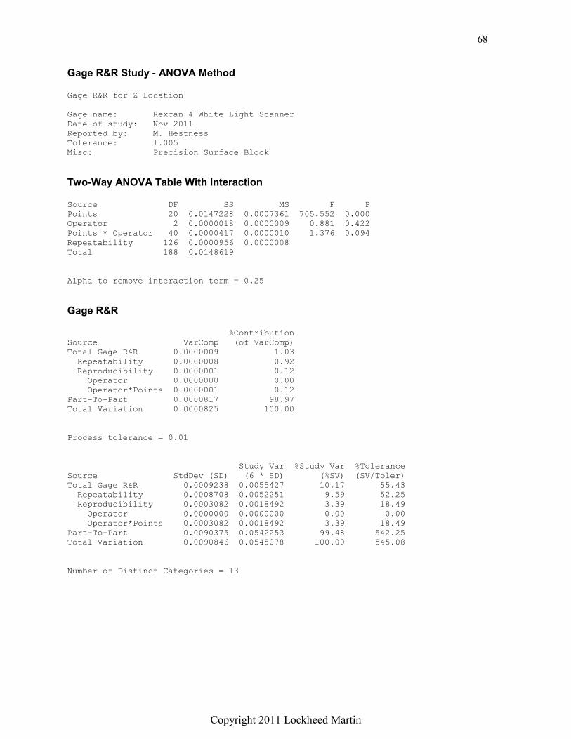
68
Copyright 2011 Lockheed Martin
Gage R&R Study - ANOVA Method Gage R&R for Z Location
Gage name: Rexcan 4 White Light Scanner
Date of study: Nov 2011
Reported by: M. Hestness
Tolerance: ±.005
Misc: Precision Surface Block
Two-Way ANOVA Table With Interaction Source DF SS MS F P
Points 20 0.0147228 0.0007361 705.552 0.000
Operator 2 0.0000018 0.0000009 0.881 0.422
Points * Operator 40 0.0000417 0.0000010 1.376 0.094
Repeatability 126 0.0000956 0.0000008
Total 188 0.0148619
Alpha to remove interaction term = 0.25
Gage R&R %Contribution
Source VarComp (of VarComp)
Total Gage R&R 0.0000009 1.03
Repeatability 0.0000008 0.92
Reproducibility 0.0000001 0.12
Operator 0.0000000 0.00
Operator*Points 0.0000001 0.12
Part-To-Part 0.0000817 98.97
Total Variation 0.0000825 100.00
Process tolerance = 0.01
Study Var %Study Var %Tolerance
Source StdDev (SD) (6 * SD) (%SV) (SV/Toler)
Total Gage R&R 0.0009238 0.0055427 10.17 55.43
Repeatability 0.0008708 0.0052251 9.59 52.25
Reproducibility 0.0003082 0.0018492 3.39 18.49
Operator 0.0000000 0.0000000 0.00 0.00
Operator*Points 0.0003082 0.0018492 3.39 18.49
Part-To-Part 0.0090375 0.0542253 99.48 542.25
Total Variation 0.0090846 0.0545078 100.00 545.08
Number of Distinct Categories = 13

69
Copyright 2011 Lockheed Martin
Appendix G: Input Data and Results for Spot Face Panel
CogniTens WLS 400M Input Data
Operator 1 Operator 2 Operator 3
Nominal Rep 1 Rep 2 Rep 3 Rep 1 Rep 2 Rep 3 Rep 1 Rep 2 Rep 3
-0.0006 -0.0003 -0.0012 -0.0009 -0.0023 0.0006 -0.0009 -0.0007 -0.0021 0.0012 -0.0011 -0.0006 -0.0008 -0.0005 -0.0012 -0.0005 -0.0014 -0.0011 0.0000 -0.0017 -0.0037 -0.0041 -0.0028 -0.0028 -0.0041 -0.0052 -0.0031 -0.0030 -0.0033 -0.0030 -0.0077 -0.0079 -0.0071 -0.0070 -0.0072 -0.0074 -0.0080 -0.0067 -0.0065 -0.0058 -0.0115 -0.0108 -0.0111 -0.0110 -0.0118 -0.0113 -0.0117 -0.0112 -0.0126 -0.0112 -0.0155 -0.0146 -0.0146 -0.0150 -0.0160 -0.0148 -0.0143 -0.0161 -0.0157 -0.0156 -0.0194 -0.0196 -0.0189 -0.0190 -0.0201 -0.0196 -0.0192 -0.0200 -0.0193 -0.0197 -0.0009 -0.0018 -0.0012 -0.0009 -0.0007 -0.0010 -0.0009 -0.0014 -0.0017 -0.0009 -0.0016 -0.0017 -0.0014 -0.0024 -0.0021 -0.0023 -0.0021 -0.0014 -0.0018 -0.0014 -0.0035 -0.0033 -0.0040 -0.0039 -0.0045 -0.0052 -0.0039 -0.0030 -0.0037 -0.0035 -0.0076 -0.0078 -0.0075 -0.0079 -0.0069 -0.0069 -0.0073 -0.0076 -0.0074 -0.0072 -0.0107 -0.0106 -0.0110 -0.0112 -0.0107 -0.0109 -0.0102 -0.0112 -0.0105 -0.0103 -0.0156 -0.0157 -0.0155 -0.0159 -0.0160 -0.0146 -0.0159 -0.0156 -0.0156 -0.0157 -0.0194 -0.0204 -0.0194 -0.0189 -0.0194 -0.0187 -0.0192 -0.0184 -0.0190 -0.0198 -0.0014 -0.0011 -0.0013 -0.0011 -0.0015 -0.0016 -0.0013 -0.0014 -0.0010 -0.0013 -0.0019 -0.0016 -0.0014 -0.0018 -0.0017 -0.0016 -0.0015 -0.0017 -0.0015 -0.0013 -0.0034 -0.0032 -0.0034 -0.0034 -0.0034 -0.0036 -0.0034 -0.0031 -0.0032 -0.0035 -0.0075 -0.0075 -0.0077 -0.0074 -0.0078 -0.0077 -0.0074 -0.0076 -0.0073 -0.0078 -0.0118 -0.0115 -0.0113 -0.0117 -0.0117 -0.0114 -0.0116 -0.0117 -0.0117 -0.0117 -0.0158 -0.0157 -0.0156 -0.0155 -0.0155 -0.0157 -0.0156 -0.0156 -0.0155 -0.0157 -0.0190 -0.0186 -0.0188 -0.0188 -0.0189 -0.0189 -0.0187 -0.0188 -0.0192 -0.0190

70
Copyright 2011 Lockheed Martin
0.000-0.005-0.010-0.015-0.020
0.002
0.001
0.000
-0.001
-0.002
Reference Value
Bia
s
0
Regression
95% CI
Data
Avg Bias
BiasLinearity
0.8
0.4
0.0
Pe
rce
nt
C onstant 0.00002382 0.00006249 0.704
Slope -0.007155 0.005781 0.217
Predictor C oef SE C oef P
Gage Linearity
S 0.0005253 R-Sq 0.8%
Linearity 0.0002896 %Linearity 0.7
A v erage 0.0000850 0.2 0.010
-0.019425 -0.0000552 0.1 0.668
-0.0194 0.0001507 0.4 0.512
-0.019 0.0001712 0.4 0.028
-0.015775 0.0001752 0.4 0.001
-0.015625 -0.0000030 0.0 0.985
-0.01545 0.0002840 0.7 0.189
-0.0118 0.0002201 0.5 0.004
Reference Bias %Bias P
Gage Bias
Gage name: C ogniTens WLS 400M
Date of study : Nov 2011
Reported by : M. Hestness
Tolerance: -.020 to .000
Misc: Spot F ace Panel
Percent of Process Variation
Gage Linearity and Bias Study for Measured
Part-to-PartReprodRepeatGage R&R
200
100
0
Perc
ent
% Contribution
% Study Var
% Tolerance
Point
9
Point
8
Point
7
Point
6
Point
5
Point
4
Poin t
3
Point 21
Point 20
Point
2
Point 19
Point 1 8
Point 17
Point 16
Point 15
P oin t
14
Point 13
Point 12
Point 11
Point 10
Point
1
Point
9
Point
8
P oint
7
Point
6
Point
5
Point
4
Point
3
P oin t
21
Point 20
Point
2
Point 19
Point 18
Point 1 7
Point 16
Point 15
Point 14
Point 1 3
Point 12
Point 11
Point 10
Poin t
1
Point
9
Point
8
Point
7
P oin t
6
Point
5
Point
4
Point
3
Point 21
P oin t
2 0
Point
2
Point 19
Point 18
P oint
17
Point 16
Point 15
Point 14
Point 13
Point 1 2
Point 11
Point 10
Point
1
0.0030
0.0015
0.0000
Points
Sam
ple
Range
_R=0.000714
UCL=0.001838
LCL=0
Operator 1 Operator 2 Operator 3
Point 9
Point 8
Point 7
Point 6
Point 5
Point 4
P oin t
3
Poin
t 21
Poin
t 20
Point 2
Po in
t 19
Poin
t 18
Poin
t 17
Poin
t 16
Poin
t 15
Poin
t 14
Poin
t 13
Poin
t 12
Poin
t 11
Po in
t 10
Point 1
Point 9
Point 8
P oint
7
Point 6
Point 5
Point 4
Point 3
Poin
t 21
Poin
t 20
Point 2
Poin
t 19
Po in
t 18
Poin
t 17
Poin
t 16
Poin
t 15
Poin
t 14
Poin
t 13
Poin
t 12
Poin
t 11
Poin
t 10
Point 1
Point 9
Point 8
Point 7
P oin t
6
Point 5
Point 4
Point 3
Poin
t 21
Poin
t 20
Point 2
Poin
t 19
Poin
t 18
Poin
t 17
Poin
t 16
Poin
t 15
Poin
t 14
Po in
t 13
Poin
t 12
Poin
t 11
Poin
t 10
Point 1
0.00
-0.01
-0.02
Points
Sam
ple
Mean
__X=-0.00847UCL=-0.00774LCL=-0.00920
Operator 1 Operator 2 Operator 3
Point 9
Point 8
Point 7
Poin t 6
Point
5
Point 4
Point 3
Poin
t 21
Poin
t 20
Point 2
Poin
t 19
Poin
t 18
Poin
t 17
Poin
t 16
Poin
t 15
Poin
t 14
Poin
t 13
Po in
t 12
Poin
t 11
Poin
t 10
Point 1
0.00
-0.01
-0.02
Points
Operator 3Operator 2Operator 1
0.00
-0.01
-0.02
Operator
Point 9
Point 8
Point 7
Point 6
Point 5
Point 4
Point 3
Poin
t 21
Poin
t 20
Point 2
Poin
t 19
Poin
t 18
Poin
t 17
Poin
t 16
Poin
t 15
Poin
t 14
Poin
t 13
Poin
t 12
Poin
t 11
Poin
t 10
Point 1
0.00
-0.01
-0.02
Points
Avera
ge Operator 1
Operator 2
Operator 3
Operator
Gage name: C ogniTens WLS 400M
Date of study : Nov 2011
Reported by : M. Hestness
Tolerance: -.020 to .000
Misc: Spot F ace Panel
Components of Variation
R Chart by Operator
Xbar Chart by Operator
Spot Face Depth by Points
Spot Face Depth by Operator
Points * Operator Interaction
Gage R&R (ANOVA) for Spot Face Depth
.. D • • • • • • I • I
• • • I ' . . -· .. t=t--~F-t-+4 • • • ' !I • •• • • • •
• • • •
I = = . ~ ] 1~ I 1Sl:3/Sll
li*e~l 1 ~ ~ $ 1
1~1 ~D

71
Copyright 2011 Lockheed Martin
Gage R&R Study - ANOVA Method Gage R&R for Spot Face Depth
Gage name: CogniTens WLS 400M
Date of study: Nov 2011
Reported by: M. Hestness
Tolerance: -.020 to .000
Misc: Spot Face Panel
Two-Way ANOVA Table With Interaction Source DF SS MS F P
Points 20 0.0081490 0.0004075 1331.76 0.000
Operator 2 0.0000007 0.0000003 1.13 0.333
Points * Operator 40 0.0000122 0.0000003 1.29 0.148
Repeatability 126 0.0000300 0.0000002
Total 188 0.0081919
Alpha to remove interaction term = 0.25
Gage R&R %Contribution
Source VarComp (of VarComp)
Total Gage R&R 0.0000003 0.57
Repeatability 0.0000002 0.52
Reproducibility 0.0000000 0.05
Operator 0.0000000 0.00
Operator*Points 0.0000000 0.05
Part-To-Part 0.0000452 99.43
Total Variation 0.0000455 100.00
Process tolerance = 0.02
Study Var %Study Var %Tolerance
Source StdDev (SD) (6 * SD) (%SV) (SV/Toler)
Total Gage R&R 0.0005110 0.0030659 7.58 15.33
Repeatability 0.0004876 0.0029255 7.23 14.63
Reproducibility 0.0001529 0.0009173 2.27 4.59
Operator 0.0000252 0.0001510 0.37 0.75
Operator*Points 0.0001508 0.0009048 2.24 4.52
Part-To-Part 0.0067260 0.0403557 99.71 201.78
Total Variation 0.0067453 0.0404720 100.00 202.36
Number of Distinct Categories = 18
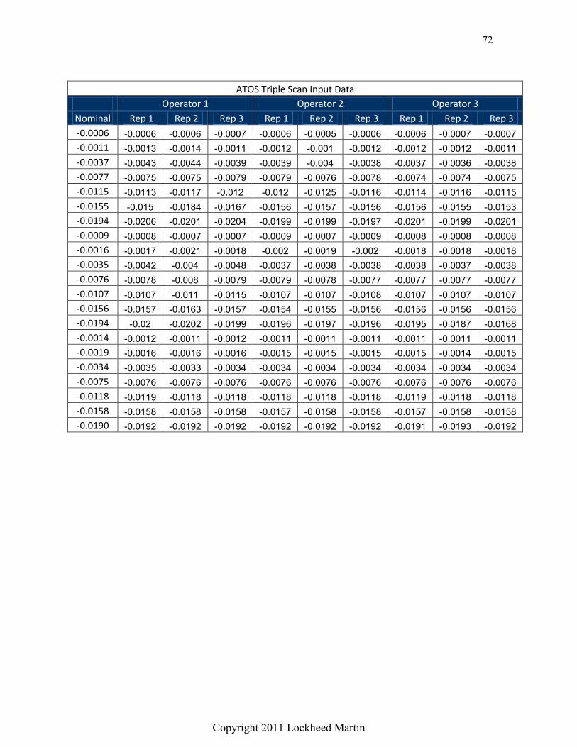
72
Copyright 2011 Lockheed Martin
ATOS Triple Scan Input Data
Operator 1 Operator 2 Operator 3
Nominal Rep 1 Rep 2 Rep 3 Rep 1 Rep 2 Rep 3 Rep 1 Rep 2 Rep 3
-0.0006 -0.0006 -0.0006 -0.0007 -0.0006 -0.0005 -0.0006 -0.0006 -0.0007 -0.0007 -0.0011 -0.0013 -0.0014 -0.0011 -0.0012 -0.001 -0.0012 -0.0012 -0.0012 -0.0011 -0.0037 -0.0043 -0.0044 -0.0039 -0.0039 -0.004 -0.0038 -0.0037 -0.0036 -0.0038 -0.0077 -0.0075 -0.0075 -0.0079 -0.0079 -0.0076 -0.0078 -0.0074 -0.0074 -0.0075 -0.0115 -0.0113 -0.0117 -0.012 -0.012 -0.0125 -0.0116 -0.0114 -0.0116 -0.0115 -0.0155 -0.015 -0.0184 -0.0167 -0.0156 -0.0157 -0.0156 -0.0156 -0.0155 -0.0153 -0.0194 -0.0206 -0.0201 -0.0204 -0.0199 -0.0199 -0.0197 -0.0201 -0.0199 -0.0201 -0.0009 -0.0008 -0.0007 -0.0007 -0.0009 -0.0007 -0.0009 -0.0008 -0.0008 -0.0008 -0.0016 -0.0017 -0.0021 -0.0018 -0.002 -0.0019 -0.002 -0.0018 -0.0018 -0.0018 -0.0035 -0.0042 -0.004 -0.0048 -0.0037 -0.0038 -0.0038 -0.0038 -0.0037 -0.0038 -0.0076 -0.0078 -0.008 -0.0079 -0.0079 -0.0078 -0.0077 -0.0077 -0.0077 -0.0077 -0.0107 -0.0107 -0.011 -0.0115 -0.0107 -0.0107 -0.0108 -0.0107 -0.0107 -0.0107 -0.0156 -0.0157 -0.0163 -0.0157 -0.0154 -0.0155 -0.0156 -0.0156 -0.0156 -0.0156 -0.0194 -0.02 -0.0202 -0.0199 -0.0196 -0.0197 -0.0196 -0.0195 -0.0187 -0.0168 -0.0014 -0.0012 -0.0011 -0.0012 -0.0011 -0.0011 -0.0011 -0.0011 -0.0011 -0.0011 -0.0019 -0.0016 -0.0016 -0.0016 -0.0015 -0.0015 -0.0015 -0.0015 -0.0014 -0.0015 -0.0034 -0.0035 -0.0033 -0.0034 -0.0034 -0.0034 -0.0034 -0.0034 -0.0034 -0.0034 -0.0075 -0.0076 -0.0076 -0.0076 -0.0076 -0.0076 -0.0076 -0.0076 -0.0076 -0.0076 -0.0118 -0.0119 -0.0118 -0.0118 -0.0118 -0.0118 -0.0118 -0.0119 -0.0118 -0.0118 -0.0158 -0.0158 -0.0158 -0.0158 -0.0157 -0.0158 -0.0158 -0.0157 -0.0158 -0.0158 -0.0190 -0.0192 -0.0192 -0.0192 -0.0192 -0.0192 -0.0192 -0.0191 -0.0193 -0.0192

73
Copyright 2011 Lockheed Martin
0.000-0.005-0.010-0.015-0.020
0.003
0.002
0.001
0.000
-0.001
-0.002
-0.003
Reference Value
Bia
s 0
Regression
95% CI
Data
Avg Bias
BiasLinearity
1.0
0.5
0.0
Pe
rce
nt
C onstant 0.00001275 0.00004894 0.795
Slope 0.013458 0.004527 0.003
Predictor C oef SE C oef P
Gage Linearity
S 0.0004114 R-Sq 4.5%
Linearity 0.0005553 %Linearity 1.3
A v erage -0.0001024 0.2 0.000
-0.019425 -0.0006528 1.6 0.000
-0.0194 0.0000667 0.2 0.861
-0.019 -0.0002000 0.5 0.000
-0.015775 -0.0000028 0.0 0.805
-0.015625 -0.0000417 0.1 0.682
-0.01545 -0.0004833 1.2 0.231
-0.0118 -0.0000222 0.1 0.079
Reference Bias %Bias P
Gage Bias
Gage name: A TO S Triple Scan
Date of study : Nov 2011
Reported by : M. Hestness
Tolerance: -.020 to .000
Misc: Spot F ace Panel
Percent of Process Variation
Gage Linearity and Bias Study for Measured
Part-to-PartReprodRepeatGage R&R
200
100
0
Perc
ent
% Contribution
% Study Var
% Tolerance
Point
9
Point
8
Point
7
Point
6
Point
5
Point
4
Poin t
3
Point 21
Point 20
Point
2
Point 19
Point 1 8
Point 17
Point 16
Point 15
P oin t
14
Point 13
Point 12
Point 11
Point 10
Point
1
Point
9
Point
8
P oint
7
Point
6
Point
5
Point
4
Point
3
P oin t
21
Point 20
Point
2
Point 19
Point 18
Point 1 7
Point 16
Point 15
Point 14
Point 1 3
Point 12
Point 11
Point 10
Poin t
1
Point
9
Point
8
Point
7
P oin t
6
Point
5
Point
4
Point
3
Point 21
P oin t
2 0
Point
2
Point 19
Point 18
P oint
17
Point 16
Point 15
Point 14
Point 13
Point 1 2
Point 11
Point 10
Point
1
0.0030
0.0015
0.0000
Points
Sam
ple
Range
_R=0.000271UCL=0.000699LCL=0
Operator 1 Operator 2 Operator 3
Point 9
Point 8
Point 7
Point 6
Point 5
Point 4
P oin t
3
Poin
t 21
Poin
t 20
Point 2
Po in
t 19
Poin
t 18
Poin
t 17
Poin
t 16
Poin
t 15
Poin
t 14
Poin
t 13
Poin
t 12
Poin
t 11
Po in
t 10
Point 1
Point 9
Point 8
P oint
7
Point 6
Point 5
Point 4
Point 3
Poin
t 21
Poin
t 20
Point 2
Poin
t 19
Po in
t 18
Poin
t 17
Poin
t 16
Poin
t 15
Poin
t 14
Poin
t 13
Poin
t 12
Poin
t 11
Poin
t 10
Point 1
Point 9
Point 8
Point 7
P oin t
6
Point 5
Point 4
Point 3
Poin
t 21
Poin
t 20
Point 2
Poin
t 19
Poin
t 18
Poin
t 17
Poin
t 16
Poin
t 15
Poin
t 14
Po in
t 13
Poin
t 12
Poin
t 11
Poin
t 10
Point 1
0.00
-0.01
-0.02
Points
Sam
ple
Mean
__X=-0.00866UCL=-0.00838LCL=-0.00893
Operator 1 Operator 2 Operator 3
Point 9
Point 8
Point 7
Poin t 6
Point
5
Point 4
Point 3
Poin
t 21
Poin
t 20
Point 2
Poin
t 19
Poin
t 18
Poin
t 17
Poin
t 16
Poin
t 15
Poin
t 14
Poin
t 13
Po in
t 12
Poin
t 11
Poin
t 10
Point 1
0.00
-0.01
-0.02
Points
Operator 3Operator 2Operator 1
0.00
-0.01
-0.02
Operator
Point 9
Point 8
Point 7
Point 6
Point 5
Point 4
Point 3
Poin
t 21
Poin
t 20
Point 2
Poin
t 19
Poin
t 18
Poin
t 17
Poin
t 16
Poin
t 15
Poin
t 14
Poin
t 13
Poin
t 12
Poin
t 11
Poin
t 10
Point 1
0.00
-0.01
-0.02
Points
Avera
ge Operator 1
Operator 2
Operator 3
Operator
Gage name: A TO S Triple Scan
Date of study : Nov 2011
Reported by : M. Hestness
Tolerance: -.020 to .000
Misc: Spot F ace Panel
Components of Variation
R Chart by Operator
Xbar Chart by Operator
Spot Face Depth by Points
Spot Face Depth by Operator
Points * Operator Interaction
Gage R&R (ANOVA) for Spot Face Depth
• D •
t=i=-A~<::4-- ·~ I : · 11 • • • • • • •
•
I .= .= . ~ 1 1~ I I'SL3/S[I
1~1

74
Copyright 2011 Lockheed Martin
Gage R&R Study - ANOVA Method Gage R&R for Spot Face Depth
Gage name: ATOS Triple Scan
Date of study: Nov 2011
Reported by: M. Hestness
Tolerance: -.020 to .000
Misc: Spot Face Panel
Two-Way ANOVA Table With Interaction Source DF SS MS F P
Points 20 0.0084910 0.0004246 2197.22 0.000
Operator 2 0.0000025 0.0000012 6.42 0.004
Points * Operator 40 0.0000077 0.0000002 1.99 0.002
Repeatability 126 0.0000122 0.0000001
Total 188 0.0085135
Alpha to remove interaction term = 0.25
Gage R&R %Contribution
Source VarComp (of VarComp)
Total Gage R&R 0.0000001 0.31
Repeatability 0.0000001 0.21
Reproducibility 0.0000000 0.10
Operator 0.0000000 0.04
Operator*Points 0.0000000 0.07
Part-To-Part 0.0000472 99.69
Total Variation 0.0000473 100.00
Process tolerance = 0.02
Study Var %Study Var %Tolerance
Source StdDev (SD) (6 * SD) (%SV) (SV/Toler)
Total Gage R&R 0.0003817 0.0022905 5.55 11.45
Repeatability 0.0003115 0.0018690 4.53 9.35
Reproducibility 0.0002207 0.0013240 3.21 6.62
Operator 0.0001290 0.0007738 1.88 3.87
Operator*Points 0.0001791 0.0010743 2.60 5.37
Part-To-Part 0.0068667 0.0412000 99.85 206.00
Total Variation 0.0068773 0.0412636 100.00 206.32
Number of Distinct Categories = 25
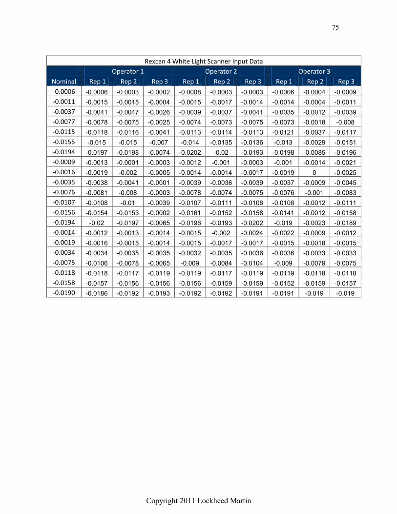
75
Copyright 2011 Lockheed Martin
Rexcan 4 White Light Scanner Input Data
Operator 1 Operator 2 Operator 3
Nominal Rep 1 Rep 2 Rep 3 Rep 1 Rep 2 Rep 3 Rep 1 Rep 2 Rep 3
-0.0006 -0.0006 -0.0003 -0.0002 -0.0008 -0.0003 -0.0003 -0.0006 -0.0004 -0.0009 -0.0011 -0.0015 -0.0015 -0.0004 -0.0015 -0.0017 -0.0014 -0.0014 -0.0004 -0.0011 -0.0037 -0.0041 -0.0047 -0.0026 -0.0039 -0.0037 -0.0041 -0.0035 -0.0012 -0.0039 -0.0077 -0.0078 -0.0075 -0.0025 -0.0074 -0.0073 -0.0075 -0.0073 -0.0018 -0.008 -0.0115 -0.0118 -0.0116 -0.0041 -0.0113 -0.0114 -0.0113 -0.0121 -0.0037 -0.0117 -0.0155 -0.015 -0.015 -0.007 -0.014 -0.0135 -0.0136 -0.013 -0.0029 -0.0151 -0.0194 -0.0197 -0.0198 -0.0074 -0.0202 -0.02 -0.0193 -0.0198 -0.0085 -0.0196 -0.0009 -0.0013 -0.0001 -0.0003 -0.0012 -0.001 -0.0003 -0.001 -0.0014 -0.0021 -0.0016 -0.0019 -0.002 -0.0005 -0.0014 -0.0014 -0.0017 -0.0019 0 -0.0025 -0.0035 -0.0038 -0.0041 -0.0001 -0.0039 -0.0036 -0.0039 -0.0037 -0.0009 -0.0045 -0.0076 -0.0081 -0.008 -0.0003 -0.0078 -0.0074 -0.0075 -0.0076 -0.001 -0.0083 -0.0107 -0.0108 -0.01 -0.0039 -0.0107 -0.0111 -0.0106 -0.0108 -0.0012 -0.0111 -0.0156 -0.0154 -0.0153 -0.0002 -0.0161 -0.0152 -0.0158 -0.0141 -0.0012 -0.0158 -0.0194 -0.02 -0.0197 -0.0065 -0.0196 -0.0193 -0.0202 -0.019 -0.0023 -0.0189 -0.0014 -0.0012 -0.0013 -0.0014 -0.0015 -0.002 -0.0024 -0.0022 -0.0009 -0.0012 -0.0019 -0.0016 -0.0015 -0.0014 -0.0015 -0.0017 -0.0017 -0.0015 -0.0018 -0.0015 -0.0034 -0.0034 -0.0035 -0.0035 -0.0032 -0.0035 -0.0036 -0.0036 -0.0033 -0.0033 -0.0075 -0.0106 -0.0078 -0.0065 -0.009 -0.0084 -0.0104 -0.009 -0.0079 -0.0075 -0.0118 -0.0118 -0.0117 -0.0119 -0.0119 -0.0117 -0.0119 -0.0119 -0.0118 -0.0118 -0.0158 -0.0157 -0.0156 -0.0156 -0.0156 -0.0159 -0.0159 -0.0152 -0.0159 -0.0157 -0.0190 -0.0186 -0.0192 -0.0193 -0.0192 -0.0192 -0.0191 -0.0191 -0.019 -0.019

76
Copyright 2011 Lockheed Martin
0.000-0.005-0.010-0.015-0.020
0.020
0.015
0.010
0.005
0.000
Reference Value
Bia
s
0
Regression
95% CI
Data
Avg Bias
BiasLinearity
10
5
0
Pe
rce
nt
C onstant -0.0001664 0.0003524 0.637
Slope -0.12061 0.03260 0.000
Predictor C oef SE C oef P
Gage Linearity
S 0.0029625 R-Sq 6.8%
Linearity 0.0048214 %Linearity 12.1
A v erage 0.0008653 2.2 0.000
-0.019425 0.0022806 5.7 0.144
-0.0194 0.0032333 8.1 0.139
-0.019 -0.0000778 0.2 0.339
-0.015775 0.0000972 0.2 0.241
-0.015625 0.0035028 8.8 0.081
-0.01545 0.0033278 8.3 0.040
-0.0118 -0.0000222 0.1 0.339
Reference Bias %Bias P
Gage Bias
Gage name: Rexcan 4 White Light Sy stem
Date of study : Nov 2011
Reported by : M. Hestness
Tolerance: -.020 to .000
Misc: Spot F ace Panel
Percent of Process Variation
Gage Linearity and Bias Study for Measured
Part-to-PartReprodRepeatGage R&R
200
100
0
Perc
ent
% Contribution
% Study Var
% Tolerance
Point
9
Point
8
Point
7
Poin t
6
Point
5
Point
4
Point
3
Point 21
Point 20
Poin t
2
Point 1 9
Point 18
Point 17
Point 16
Point 15
P oint
14
Point 1 3
Point 12
Point 11
Point 10
Point
1
Poin t
9
Point
8
Point
7
Point
6
Point
5
Point
4
Poin t
3
Point 2 1
Point 20
Point
2
Point 19
Point 18
P oint
17
Point 1 6
Point 15
Point 14
Point 13
Point 12
P oint
11
Point 1 0
Point
1
Point
9
Point
8
Point
7
Poin t
6
Point
5
Point
4
Point
3
Point 21
Point 20
Poin t
2
Point 1 9
Point 18
Point 17
Point 16
Point 15
P oint
14
Point 1 3
Point 12
Point 11
Point 10
Point
1
0.016
0.008
0.000
Points
Sam
ple
Range
_R=0.00327
UCL=0.00843
LCL=0
Operator 1 Operator 2 Operator 3
Point 9
Point 8
Point 7
Point 6
Point 5
Point 4
Point 3
Poin
t 21
Poin
t 20
Point 2
Poin
t 19
Poin
t 18
Poin
t 17
Poin
t 16
Poin
t 15
Poin
t 14
Poin
t 13
Poin
t 12
Poin
t 11
Poin
t 10
Point 1
Point 9
Point 8
Point 7
Point 6
Point 5
Point 4
Point 3
Poin
t 21
Poin
t 20
Point 2
Poin
t 19
Poin
t 18
Poin
t 17
Poin
t 16
Poin
t 15
Poin
t 14
Poin
t 13
Poin
t 12
Poin
t 11
Poin
t 10
Point 1
Point 9
Point 8
Point 7
Point 6
Point 5
Point 4
Point 3
Poin
t 21
Poin
t 20
Point 2
Poin
t 19
Poin
t 18
Poin
t 17
Poin
t 16
Poin
t 15
Poin
t 14
Poin
t 13
Poin
t 12
Poin
t 11
Poin
t 10
Point 1
0.00
-0.01
-0.02
Points
Sam
ple
Mean
__X=-0.00769UCL=-0.00434
LCL=-0.01104
Operator 1 Operator 2 Operator 3
Point 9
Point 8
Point 7
Poin t 6
Point
5
Point 4
Point 3
Poin
t 21
Poin
t 20
Point 2
Poin
t 19
Poin
t 18
Poin
t 17
Poin
t 16
Poin
t 15
Poin
t 14
Poin
t 13
Po in
t 12
Poin
t 11
Poin
t 10
Point 1
0.00
-0.01
-0.02
Points
Operator 3Operator 2Operator 1
0.00
-0.01
-0.02
Operator
Point 9
Point 8
Point 7
Point 6
Point 5
Point 4
Point 3
Poin
t 21
Poin
t 20
Point 2
Poin
t 19
Poin
t 18
Poin
t 17
Poin
t 16
Poin
t 15
Poin
t 14
Poin
t 13
Poin
t 12
Poin
t 11
Poin
t 10
Point 1
0.00
-0.01
-0.02
Points
Avera
ge Operator 1
Operator 2
Operator 3
Operator
Gage name: Rexcan 4 White Light Scanner
Date of study : Nov 2011
Reported by : M. Hestness
Tolerance: -020 to .000
Misc: Spot F ace Panel
Components of Variation
R Chart by Operator
Xbar Chart by Operator
Spot Face Depth by Points
Spot Face Depth by Operator
Points * Operator Interaction
Gage R&R (ANOVA) for Spot Face Depth

77
Copyright 2011 Lockheed Martin
Gage R&R Study - ANOVA Method Gage R&R for Spot Face Depth
Gage name: Rexcan 4 White Light Scanner
Date of study: Nov 2011
Reported by: M. Hestness
Tolerance: -020 to .000
Misc: Spot Face Panel
Two-Way ANOVA Table With Interaction Source DF SS MS F P
Points 20 0.0065752 0.0003288 98.2336 0.000
Operator 2 0.0000841 0.0000420 12.5591 0.000
Points * Operator 40 0.0001339 0.0000033 0.3416 1.000
Repeatability 126 0.0012343 0.0000098
Total 188 0.0080275
Alpha to remove interaction term = 0.25
Two-Way ANOVA Table Without Interaction Source DF SS MS F P
Points 20 0.0065752 0.0003288 39.8891 0.000
Operator 2 0.0000841 0.0000420 5.0998 0.007
Repeatability 166 0.0013682 0.0000082
Total 188 0.0080275
Gage R&R %Contribution
Source VarComp (of VarComp)
Total Gage R&R 0.0000088 19.77
Repeatability 0.0000082 18.57
Reproducibility 0.0000005 1.21
Operator 0.0000005 1.21
Part-To-Part 0.0000356 80.23
Total Variation 0.0000444 100.00
Process tolerance = 0.02
Study Var %Study Var %Tolerance
Source StdDev (SD) (6 * SD) (%SV) (SV/Toler)
Total Gage R&R 0.0029628 0.0177769 44.47 88.88
Repeatability 0.0028709 0.0172252 43.09 86.13
Reproducibility 0.0007324 0.0043942 10.99 21.97
Operator 0.0007324 0.0043942 10.99 21.97
Part-To-Part 0.0059677 0.0358061 89.57 179.03
Total Variation 0.0066627 0.0399762 100.00 199.88
Number of Distinct Categories = 2

78
Copyright 2011 Lockheed Martin
Appendix H: Input Data and Results for Countersink Panel
CogniTens WLS 400M Input Data
Operator 1 Operator 2 Operator 3
Nominal Diam. Rep 1 Rep 2 Rep 3 Rep 1 Rep 2 Rep 3 Rep 1 Rep 2 Rep 3
0.3764 0.3903 0.3878 0.3850 0.3846 0.3901 0.3886 0.3867 0.3920 0.3889
0.507 0.4455 0.4465 0.4441 0.4431 0.4465 0.4457 0.4462 0.4467 0.4475
0.5781 0.5742 0.5740 0.5720 0.5701 0.5744 0.5739 0.5733 0.5739 0.5752
0.401 0.3985 0.3971 0.3956 0.3944 0.3983 0.3965 0.3944 0.3972 0.3976
0.5286 0.5246 0.5237 0.5205 0.5222 0.5242 0.5208 0.5190 0.5216 0.5234
0.6403 0.6492 0.6490 0.6462 0.6448 0.6492 0.6451 0.6454 0.6472 0.6474
0.7778 0.7777 0.7790 0.7755 0.7741 0.7767 0.7735 0.7772 0.7760 0.7730
0.3709 0.3807 0.3780 0.3780 0.3806 0.3810 0.3806 0.3793 0.3817 0.3812
0.4443 0.4484 0.4457 0.4461 0.4466 0.4453 0.4465 0.4457 0.4443 0.4423
0.5726 0.6444 0.6431 0.6434 0.6428 0.6425 0.6431 0.6436 0.6449 0.6440
0.3954 0.3935 0.3815 0.3908 0.3905 0.3897 0.3890 0.3872 0.3906 0.3909
0.5199 0.5262 0.5235 0.5221 0.5223 0.5223 0.5210 0.5224 0.5231 0.5134
0.6399 0.6486 0.6464 0.6439 0.6454 0.6462 0.6440 0.6465 0.6447 0.6463
0.7756 0.7819 0.7776 0.7770 0.7778 0.7767 0.7743 0.7802 0.7783 0.7770
0.374 0.3706 0.3651 0.3681 0.3697 0.3685 0.3675 0.3675 0.3688 0.3709
0.4495 0.4407 0.4367 0.4375 0.4373 0.4351 0.4376 0.4359 0.4389 0.4381
0.5692 0.6420 0.6385 0.6388 0.6395 0.6358 0.6374 0.6381 0.6397 0.6385
0.396 0.3871 0.3820 0.3828 0.3840 0.3824 0.3815 0.3826 0.3841 0.3826
0.5218 0.5175 0.5215 0.5151 0.5209 0.5188 0.5192 0.5195 0.5220 0.5204
0.6464 0.6478 0.6463 0.6460 0.6439 0.6436 0.6437 0.6440 0.6469 0.6444
0.7747 0.7820 0.7766 0.7698 0.7760 0.7677 0.7716 0.7707 0.7729 0.7737
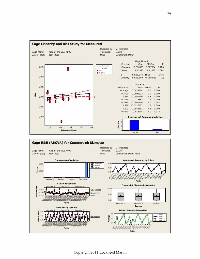
79
Copyright 2011 Lockheed Martin
0.80.70.60.50.4
0.075
0.050
0.025
0.000
-0.025
-0.050
Reference Value
Bia
s
0
Regression
95% CI
Data
Avg Bias
BiasLinearity
2
1
0
Pe
rce
nt
C onstant -0.010525 0.007934 0.186
Slope 0.02495 0.01437 0.084
Predictor C oef SE C oef P
Gage Linearity
S 0.0260344 R-Sq 1.6%
Linearity 0.0210960 %Linearity 2.5
A v erage 0.0028508 0.3 0.000
0.3709 0.0092222 1.1 0.000
0.374 -0.0054749 0.6 0.000
0.3764 0.0118382 1.4 0.000
0.3954 -0.0061149 0.7 0.002
0.396 -0.0127627 1.5 0.000
0.401 -0.0043691 0.5 0.000
0.4443 0.0013604 0.2 0.078
Reference Bias %Bias P
Gage Bias
Gage name: C ogniTens WLS 400M
Date of study : Nov 2011
Reported by : M. Hestness
Tolerance: ±.010
Misc: C ountersink Panel
Percent of Process Variation
Gage Linearity and Bias Study for Measured
Part-to-PartReprodRepeatGage R&R
4000
2000
0
Perc
ent
% Contribution
% Study Var
% Tolerance
Point
9
Point
8
Point
7
Poin t
6
Point
5
Point
4
Point
3
Point 21
Point 20
Poin t
2
Point 1 9
Point 18
Point 17
Point 16
Point 15
P oint
14
Point 1 3
Point 12
Point 11
Point 10
Point
1
Poin t
9
Point
8
Point
7
Point
6
Point
5
Point
4
Poin t
3
Point 2 1
Point 20
Point
2
Point 19
Point 18
P oint
17
Point 1 6
Point 15
Point 14
Point 13
Point 12
P oint
11
Point 1 0
Point
1
Point
9
Point
8
Point
7
Poin t
6
Point
5
Point
4
Point
3
Point 21
Point 20
Poin t
2
Point 1 9
Point 18
Point 17
Point 16
Point 15
P oint
14
Point 1 3
Point 12
Point 11
Point 10
Point
1
0.010
0.005
0.000
Points
Sam
ple
Range
_R=0.00350
UCL=0.00902
LCL=0
Operator 1 Operator 2 Operator 3
Point 9
Point 8
Point 7
Point 6
Point 5
Point 4
Point 3
Poin
t 21
Poin
t 20
Point 2
Poin
t 19
Poin
t 18
Poin
t 17
Poin
t 16
Poin
t 15
Poin
t 14
Poin
t 13
Poin
t 12
Poin
t 11
Poin
t 10
Point 1
Point 9
Point 8
Point 7
Point 6
Point 5
Point 4
Point 3
Poin
t 21
Poin
t 20
Point 2
Poin
t 19
Poin
t 18
Poin
t 17
Poin
t 16
Poin
t 15
Poin
t 14
Poin
t 13
Poin
t 12
Poin
t 11
Poin
t 10
Point 1
Point 9
Point 8
Point 7
Point 6
Point 5
Point 4
Point 3
Poin
t 21
Poin
t 20
Point 2
Poin
t 19
Poin
t 18
Poin
t 17
Poin
t 16
Poin
t 15
Poin
t 14
Poin
t 13
Poin
t 12
Poin
t 11
Poin
t 10
Point 1
0.8
0.6
0.4
Points
Sam
ple
Mean
__X=0.5390UCL=0.5426LCL=0.5354
Operator 1 Operator 2 Operator 3
Point 9
Poi n
t 8
Point 7
Point 6
Poi nt 5
Point 4
Poi n
t 3
Poi nt 2
1
Point 2
0
Poi nt 2
Point 1
9
Point 1
8
Poi nt 1
7
Point 1
6
Poi n
t 15
Point 1
4
Point 1
3
Poi nt 1
2
Point 1
1
Poi n
t 10
Point 1
0.8
0.6
0.4
Points
Operator 3Operator 2Operator 1
0.8
0.6
0.4
Operator
Point 9
P oint
8
Point 7
Point 6
P oin t 5
Point 4
Point 3
Poin
t 21
Poin
t 20
Point 2
Poin
t 19
Poin
t 18
Poin
t 17
Poin
t 16
Poin
t 15
Poin
t 14
Poin
t 13
Poin
t 12
Poin
t 11
Poin
t 10
P oint
1
0.8
0.6
0.4
Points
Avera
ge
Operator 1
Operator 2
Operator 3
Operator
Gage name: C ogniTens WLS 400M
Date of study : Nov 2011
Reported by : M. Hestness
Tolerance: ±.010
Misc: C ountersink Panel Point
Components of Variation
R Chart by Operator
Xbar Chart by Operator
Countersink Diameter by Points
Countersink Diameter by Operator
Points * Operator Interaction
Gage R&R (ANOVA) for Countersink Diameter
• D
I
1 m~ I 11'21&ZSZkl
I~ ~ ~I ~I lfZ)f&ZS1JD

80
Copyright 2011 Lockheed Martin
Gage R&R Study - ANOVA Method Gage R&R for Countersink Diameter
Gage name: CogniTens WLS 400M
Date of study: Nov 2011
Reported by: M. Hestness
Tolerance: ±.010
Misc: Countersink Panel Point
Two-Way ANOVA Table With Interaction Source DF SS MS F P
Points 20 3.57451 0.178725 50592.6 0.000
Operator 2 0.00003 0.000016 4.4 0.018
Points * Operator 40 0.00014 0.000004 0.7 0.859
Repeatability 126 0.00060 0.000005
Total 188 3.57528
Alpha to remove interaction term = 0.25
Two-Way ANOVA Table Without Interaction Source DF SS MS F P
Points 20 3.57451 0.178725 40100.8 0.000
Operator 2 0.00003 0.000016 3.5 0.032
Repeatability 166 0.00074 0.000004
Total 188 3.57528
Gage R&R %Contribution
Source VarComp (of VarComp)
Total Gage R&R 0.0000046 0.02
Repeatability 0.0000045 0.02
Reproducibility 0.0000002 0.00
Operator 0.0000002 0.00
Part-To-Part 0.0198579 99.98
Total Variation 0.0198625 100.00
Process tolerance = 0.02
Study Var %Study Var %Tolerance
Source StdDev (SD) (6 * SD) (%SV) (SV/Toler)
Total Gage R&R 0.002153 0.012917 1.53 64.58
Repeatability 0.002111 0.012667 1.50 63.33
Reproducibility 0.000421 0.002528 0.30 12.64
Operator 0.000421 0.002528 0.30 12.64
Part-To-Part 0.140918 0.845508 99.99 4227.54
Total Variation 0.140934 0.845606 100.00 4228.03
Number of Distinct Categories = 92
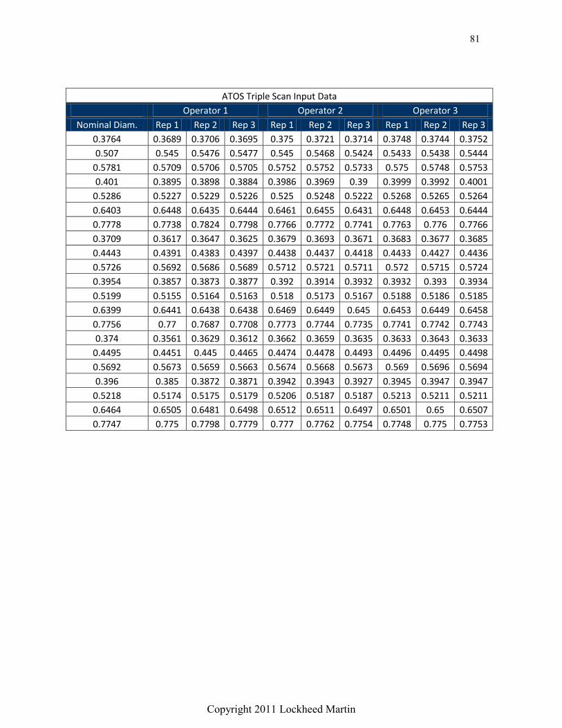
81
Copyright 2011 Lockheed Martin
ATOS Triple Scan Input Data
Operator 1 Operator 2 Operator 3
Nominal Diam. Rep 1 Rep 2 Rep 3 Rep 1 Rep 2 Rep 3 Rep 1 Rep 2 Rep 3
0.3764 0.3689 0.3706 0.3695 0.375 0.3721 0.3714 0.3748 0.3744 0.3752
0.507 0.545 0.5476 0.5477 0.545 0.5468 0.5424 0.5433 0.5438 0.5444
0.5781 0.5709 0.5706 0.5705 0.5752 0.5752 0.5733 0.575 0.5748 0.5753
0.401 0.3895 0.3898 0.3884 0.3986 0.3969 0.39 0.3999 0.3992 0.4001
0.5286 0.5227 0.5229 0.5226 0.525 0.5248 0.5222 0.5268 0.5265 0.5264
0.6403 0.6448 0.6435 0.6444 0.6461 0.6455 0.6431 0.6448 0.6453 0.6444
0.7778 0.7738 0.7824 0.7798 0.7766 0.7772 0.7741 0.7763 0.776 0.7766
0.3709 0.3617 0.3647 0.3625 0.3679 0.3693 0.3671 0.3683 0.3677 0.3685
0.4443 0.4391 0.4383 0.4397 0.4438 0.4437 0.4418 0.4433 0.4427 0.4436
0.5726 0.5692 0.5686 0.5689 0.5712 0.5721 0.5711 0.572 0.5715 0.5724
0.3954 0.3857 0.3873 0.3877 0.392 0.3914 0.3932 0.3932 0.393 0.3934
0.5199 0.5155 0.5164 0.5163 0.518 0.5173 0.5167 0.5188 0.5186 0.5185
0.6399 0.6441 0.6438 0.6438 0.6469 0.6449 0.645 0.6453 0.6449 0.6458
0.7756 0.77 0.7687 0.7708 0.7773 0.7744 0.7735 0.7741 0.7742 0.7743
0.374 0.3561 0.3629 0.3612 0.3662 0.3659 0.3635 0.3633 0.3643 0.3633
0.4495 0.4451 0.445 0.4465 0.4474 0.4478 0.4493 0.4496 0.4495 0.4498
0.5692 0.5673 0.5659 0.5663 0.5674 0.5668 0.5673 0.569 0.5696 0.5694
0.396 0.385 0.3872 0.3871 0.3942 0.3943 0.3927 0.3945 0.3947 0.3947
0.5218 0.5174 0.5175 0.5179 0.5206 0.5187 0.5187 0.5213 0.5211 0.5211
0.6464 0.6505 0.6481 0.6498 0.6512 0.6511 0.6497 0.6501 0.65 0.6507
0.7747 0.775 0.7798 0.7779 0.777 0.7762 0.7754 0.7748 0.775 0.7753

82
Copyright 2011 Lockheed Martin
0.80.70.60.50.4
0.04
0.03
0.02
0.01
0.00
-0.01
-0.02
Reference Value
Bia
s
0
Regression
95% CI
Data
Avg Bias
BiasLinearity
1.6
0.8
0.0
Pe
rce
nt
C onstant -0.008111 0.002879 0.005
Slope 0.014522 0.005214 0.006
Predictor C oef SE C oef P
Gage Linearity
S 0.0094474 R-Sq 4.0%
Linearity 0.0119675 %Linearity 1.5
A v erage -0.0003249 0.0 0.026
0.3709 -0.0044889 0.5 0.001
0.374 -0.0110333 1.3 0.000
0.3764 -0.0039667 0.5 0.001
0.3954 -0.0046333 0.6 0.001
0.396 -0.0044000 0.5 0.004
0.401 -0.0062889 0.8 0.002
0.4443 -0.0025222 0.3 0.004
Reference Bias %Bias P
Gage Bias
Gage name: A TO S Triple Scan
Date of study : Nov 2011
Reported by : M. Hestness
Tolerance: ±.010
Misc: C ountersink Panel
Percent of Process Variation
Gage Linearity and Bias Study for Measured
Part-to-PartReprodRepeatGage R&R
4000
2000
0
Perc
ent
% Contribution
% Study Var
% Tolerance
Point
9
Point
8
Point
7
Poin t
6
Point
5
Point
4
Point
3
Point 21
Point 20
Poin t
2
Point 1 9
Point 18
Point 17
Point 16
Point 15
P oint
14
Point 1 3
Point 12
Point 11
Point 10
Point
1
Poin t
9
Point
8
Point
7
Point
6
Point
5
Point
4
Poin t
3
Point 2 1
Point 20
Point
2
Point 19
Point 18
P oint
17
Point 1 6
Point 15
Point 14
Point 13
Point 12
P oint
11
Point 1 0
Point
1
Point
9
Point
8
Point
7
Poin t
6
Point
5
Point
4
Point
3
Point 21
Point 20
Poin t
2
Point 1 9
Point 18
Point 17
Point 16
Point 15
P oint
14
Point 1 3
Point 12
Point 11
Point 10
Point
1
0.008
0.004
0.000
Points
Sam
ple
Range
_R=0.001789
UCL=0.004605
LCL=0
Operator 1 Operator 2 Operator 3
Point 9
Point 8
Point 7
Point 6
Point 5
Point 4
Point 3
Poin
t 21
Poin
t 20
Point 2
Poin
t 19
Poin
t 18
Poin
t 17
Poin
t 16
Poin
t 15
Poin
t 14
Poin
t 13
Poin
t 12
Poin
t 11
Poin
t 10
Point 1
Point 9
Point 8
Point 7
Point 6
Point 5
Point 4
Point 3
Poin
t 21
Poin
t 20
Point 2
Poin
t 19
Poin
t 18
Poin
t 17
Poin
t 16
Poin
t 15
Poin
t 14
Poin
t 13
Poin
t 12
Poin
t 11
Poin
t 10
Point 1
Point 9
Point 8
Point 7
Point 6
Point 5
Point 4
Point 3
Poin
t 21
Poin
t 20
Point 2
Poin
t 19
Poin
t 18
Poin
t 17
Poin
t 16
Poin
t 15
Poin
t 14
Poin
t 13
Poin
t 12
Poin
t 11
Poin
t 10
Point 1
0.8
0.6
0.4
Points
Sam
ple
Mean
__X=0.5358UCL=0.5377LCL=0.5340
Operator 1 Operator 2 Operator 3
Point 9
Poi n
t 8
Point 7
Point 6
Poi nt 5
Point 4
Poi n
t 3
Poi nt 2
1
Point 2
0
Poi nt 2
Point 1
9
Point 1
8
Poi nt 1
7
Point 1
6
Poi n
t 15
Point 1
4
Point 1
3
Poi nt 1
2
Point 1
1
Poi n
t 10
Point 1
0.8
0.6
0.4
Points
Operator 3Operator 2Operator 1
0.8
0.6
0.4
Operator
Point 9
P oint
8
Point 7
Point 6
P oin t 5
Point 4
Point 3
Poin
t 21
Poin
t 20
Point 2
Poin
t 19
Poin
t 18
Poin
t 17
Poin
t 16
Poin
t 15
Poin
t 14
Poin
t 13
Poin
t 12
Poin
t 11
Poin
t 10
P oint
1
0.8
0.6
0.4
Points
Avera
ge
Operator 1
Operator 2
Operator 3
Operator
Gage name: A TO S Triple Scan
Date of study : Nov 2011
Reported by : M. Hestness
Tolerance: ±.010
Misc: C ountersink Panel
Components of Variation
R Chart by Operator
Xbar Chart by Operator
Countersink Diameter by Points
Countersink Diameter by Operator
Points * Operator Interaction
Gage R&R (ANOVA) for Countersink Diameter
I I:- I
•
1 ... m~ ~~~~
~I

83
Copyright 2011 Lockheed Martin
Gage R&R Study - ANOVA Method Gage R&R for Countersink Diameter
Gage name: ATOS Triple Scan
Date of study: Nov 2011
Reported by: M. Hestness
Tolerance: ±.010
Misc: Countersink Panel
Two-Way ANOVA Table With Interaction Source DF SS MS F P
Points 20 3.39445 0.169722 16786.1 0.000
Operator 2 0.00035 0.000177 17.5 0.000
Points * Operator 40 0.00040 0.000010 5.9 0.000
Repeatability 126 0.00022 0.000002
Total 188 3.39542
Alpha to remove interaction term = 0.25
Gage R&R %Contribution
Source VarComp (of VarComp)
Total Gage R&R 0.0000072 0.04
Repeatability 0.0000017 0.01
Reproducibility 0.0000054 0.03
Operator 0.0000027 0.01
Operator*Points 0.0000028 0.01
Part-To-Part 0.0188569 99.96
Total Variation 0.0188641 100.00
Process tolerance = 0.02
Study Var %Study Var %Tolerance
Source StdDev (SD) (6 * SD) (%SV) (SV/Toler)
Total Gage R&R 0.002678 0.016066 1.95 80.33
Repeatability 0.001313 0.007876 0.96 39.38
Reproducibility 0.002334 0.014003 1.70 70.01
Operator 0.001628 0.009768 1.19 48.84
Operator*Points 0.001672 0.010033 1.22 50.16
Part-To-Part 0.137320 0.823923 99.98 4119.61
Total Variation 0.137347 0.824079 100.00 4120.40
Number of Distinct Categories = 72

84
Copyright 2011 Lockheed Martin
Rexcan 4 White Light Scanner Input Data
Operator 1 Operator 2 Operator 3
Nominal Diam. Rep 1 Rep 2 Rep 3 Rep 1 Rep 2 Rep 3 Rep 1 Rep 2 Rep 3
0.3764 0.3838 0.3726 0.3708 0.3808 0.3803 0.3803 0.3685 0.3829 0.373
0.507 0.5417 0.5401 0.5379 0.543 0.5446 0.5442 0.5497 0.5366 0.5426
0.5781 0.5715 0.569 0.572 0.5785 0.5753 0.5824 0.5733 0.5758 0.5746
0.401 0.4026 0.3979 0.4008 0.4018 0.4058 0.4075 0.4032 0.402 0.4041
0.5286 0.5342 0.5226 0.5285 0.5262 0.5343 0.5323 0.5274 0.5273 0.5256
0.6403 0.6389 0.6384 0.6365 0.6453 0.6473 0.6438 0.6334 0.6433 0.639
0.7778 0.7767 0.771 0.7772 0.7746 0.7864 0.779 0.7731 0.7756 0.7809
0.3709 0.3677 0.3656 0.3664 0.3755 0.3842 0.3779 0.3601 0.3738 0.3605
0.4443 0.4415 0.4387 0.4329 0.4547 0.4522 0.4662 0.4355 0.4493 0.4361
0.5726 0.57 0.5654 0.5661 0.5731 0.5787 0.5776 0.566 0.5741 0.571
0.3954 0.3923 0.391 0.3904 0.3946 0.3985 0.4002 0.3894 0.3944 0.3883
0.5199 0.5173 0.5158 0.515 0.5224 0.5229 0.5281 0.5157 0.5199 0.5143
0.6399 0.6409 0.6402 0.6384 0.6468 0.6522 0.653 0.6425 0.6492 0.6427
0.7756 0.7716 0.7683 0.7648 0.7761 0.7775 0.7832 0.7704 0.7767 0.7692
0.374 0.3595 0.3604 0.3662 0.368 0.3766 0.3744 0.3509 0.3646 0.356
0.4495 0.4573 0.4578 0.4557 0.4582 0.4648 0.4582 0.4444 0.4556 0.4449
0.5692 0.5675 0.573 0.5754 0.577 0.5761 0.5755 0.5653 0.5742 0.5621
0.396 0.3902 0.392 0.3975 0.3955 0.4006 0.4022 0.3893 0.3993 0.3875
0.5218 0.518 0.5229 0.5234 0.5236 0.5237 0.5274 0.5207 0.5272 0.5123
0.6464 0.6468 0.6503 0.6479 0.6499 0.6557 0.651 0.6456 0.651 0.6465
0.7747 0.7752 0.7777 0.7719 0.7754 0.78 0.7781 0.7722 0.7788 0.7756

85
Copyright 2011 Lockheed Martin
0.80.70.60.50.4
0.05
0.04
0.03
0.02
0.01
0.00
-0.01
-0.02
Reference Value
Bia
s
0
Regression
95% CI
Data
Avg Bias
BiasLinearity
0.2
0.1
0.0
Pe
rce
nt
C onstant 0.000738 0.002970 0.804
Slope 0.001714 0.005379 0.750
Predictor C oef SE C oef P
Gage Linearity
S 0.0097462 R-Sq 0.1%
Linearity 0.0013954 %Linearity 0.2
A v erage 0.0016571 0.2 0.000
0.3709 -0.0007111 0.1 0.793
0.374 -0.0099333 1.2 0.009
0.3764 0.0006000 0.1 0.728
0.3954 -0.0021667 0.3 0.137
0.396 -0.0011000 0.1 0.512
0.401 0.0018556 0.2 0.117
0.4443 0.0009333 0.1 0.803
Reference Bias %Bias P
Gage Bias
Gage name: Rexcan 4 White Light Sy stem
Date of study : Nov 2011
Reported by : M. Hestness
Tolerance: ±.010
Misc: C ountersink Panel
Percent of Process Variation
Gage Linearity and Bias Study for Measured
Part-to-PartReprodRepeatGage R&R
4000
2000
0
Perc
ent
% Contribution
% Study Var
% Tolerance
Point
9
Point
8
Point
7
Point
6
Poin t
5
Point
4
Point
3
Point 21
Point 20
Point
2
Point 19
Point 18
P oin t
17
Point 1 6
Point 15
Point 14
Point 13
Point 12
Point 11
Point 10
Point
1
Point
9
Point
8
Point
7
Point
6
Point
5
P oint
4
Poin t
3
Point 2 1
Point 20
Point
2
Point 19
Point 18
Point 17
Point 16
P oin t
15
Point 1 4
Point 13
Point 12
Point 11
Point 10
Point
1
Poin t
9
Point
8
Point
7
Point
6
Point
5
Point
4
Point
3
Point 21
P oin t
20
Point
2
Point 19
Point 18
Point 17
Point 16
Point 15
Point 14
P oin t
1 3
Point 12
Point 11
Point 10
Point
1
0.02
0.01
0.00
Points
Sam
ple
Range
_R=0.00682
UCL=0.01756
LCL=0
Operator 1 Operator 2 Operator 3
Point 9
Point 8
Point 7
Point 6
P oin t
5
Point 4
Point 3
Poin
t 21
Poin
t 20
Point 2
Poin
t 19
Po in
t 18
Poin
t 17
Poin
t 16
Poin
t 15
Poin
t 14
Poin
t 13
Poin
t 12
Poin
t 11
Po in
t 10
Point 1
Point 9
Point 8
Point 7
Point 6
Point 5
P oint
4
Point 3
Poin
t 21
Poin
t 20
Point 2
Poin
t 19
Poin
t 18
Poin
t 17
Po in
t 16
Poin
t 15
Poin
t 14
Poin
t 13
Poin
t 12
Poin
t 11
Poin
t 10
Point 1
P oin t
9
Point 8
Point 7
Point 6
Point 5
Point 4
Point 3
Po in
t 21
Poin
t 20
Point 2
Poin
t 19
Poin
t 18
Poin
t 17
Poin
t 16
Poin
t 15
Po in
t 14
Poin
t 13
Poin
t 12
Poin
t 11
Poin
t 10
Point 1
0.8
0.6
0.4
Points
Sam
ple
Mean
__X=0.5378UCL=0.5448LCL=0.5308
Operator 1 Operator 2 Operator 3
Point 9
Poi n
t 8
Point 7
Point 6
Poi nt 5
Point 4
Poi n
t 3
Poi nt 2
1
Point 2
0
Poi nt 2
Point 1
9
Point 1
8
Poi nt 1
7
Point 1
6
Poi n
t 15
Point 1
4
Point 1
3
Poi nt 1
2
Point 1
1
Poi n
t 10
Point 1
0.8
0.6
0.4
Points
Operator 3Operator 2Operator 1
0.8
0.6
0.4
Operator
Point 9
P oint
8
Point 7
Point 6
P oin t 5
Point 4
Point 3
Poin
t 21
Poin
t 20
Point 2
Poin
t 19
Poin
t 18
Poin
t 17
Poin
t 16
Poin
t 15
Poin
t 14
Poin
t 13
Poin
t 12
Poin
t 11
Poin
t 10
P oint
1
0.8
0.6
0.4
Points
Avera
ge
Operator 1
Operator 2
Operator 3
Operator
Gage name: Rexcan 4 White Light Scanner
Date of study : Nov 2011
Reported by : M. Hestness
Tolerance: ±.010
Misc: C ountersink Panel
Components of Variation
R Chart by Operator
Xbar Chart by Operator
Countersink Diameter by Points
Countersink Diameter by Operator
Points * Operator Interaction
Gage R&R (ANOVA) for Countersink Diameter
D
lj~ I
I$ $ $1 ~EJ

86
Copyright 2011 Lockheed Martin
Gage R&R Study - ANOVA Method Gage R&R for Countersink Diameter
Gage name: Rexcan 4 White Light Scanner
Date of study: Nov 2011
Reported by: M. Hestness
Tolerance: ±.010
Misc: Countersink Panel
Two-Way ANOVA Table With Interaction Source DF SS MS F P
Points 20 3.30650 0.165325 6759.36 0.000
Operator 2 0.00212 0.001061 43.40 0.000
Points * Operator 40 0.00098 0.000024 1.45 0.063
Repeatability 126 0.00213 0.000017
Total 188 3.31172
Alpha to remove interaction term = 0.25
Gage R&R %Contribution
Source VarComp (of VarComp)
Total Gage R&R 0.0000359 0.19
Repeatability 0.0000169 0.09
Reproducibility 0.0000190 0.10
Operator 0.0000165 0.09
Operator*Points 0.0000025 0.01
Part-To-Part 0.0183667 99.81
Total Variation 0.0184026 100.00
Process tolerance = 0.02
Study Var %Study Var %Tolerance
Source StdDev (SD) (6 * SD) (%SV) (SV/Toler)
Total Gage R&R 0.005988 0.035929 4.41 179.64
Repeatability 0.004107 0.024641 3.03 123.21
Reproducibility 0.004358 0.026148 3.21 130.74
Operator 0.004057 0.024343 2.99 121.72
Operator*Points 0.001591 0.009545 1.17 47.73
Part-To-Part 0.135524 0.813143 99.90 4065.71
Total Variation 0.135656 0.813936 100.00 4069.68
Number of Distinct Categories = 31