a closer look at few shot classification

Published as a conference paper at ICLR 2019

A CLOSER LOOK AT FEW-SHOT CLASSIFICATION

Wei-Yu ChenCarnegie Mellon [email protected]

Yen-Cheng Liu & Zsolt KiraGeorgia Tech{ycliu,zkira}@gatech.edu

Yu-Chiang Frank WangNational Taiwan [email protected]

Jia-Bin HuangVirginia [email protected]

ABSTRACT

Few-shot classification aims to learn a classifier to recognize unseen classes duringtraining with limited labeled examples. While significant progress has been made,the growing complexity of network designs, meta-learning algorithms, and differ-ences in implementation details make a fair comparison difficult. In this paper,we present 1) a consistent comparative analysis of several representative few-shotclassification algorithms, with results showing that deeper backbones significantlyreduce the performance differences among methods on datasets with limited do-main differences, 2) a modified baseline method that surprisingly achieves com-petitive performance when compared with the state-of-the-art on both the mini-ImageNet and the CUB datasets, and 3) a new experimental setting for evaluatingthe cross-domain generalization ability for few-shot classification algorithms. Ourresults reveal that reducing intra-class variation is an important factor when thefeature backbone is shallow, but not as critical when using deeper backbones. Ina realistic cross-domain evaluation setting, we show that a baseline method witha standard fine-tuning practice compares favorably against other state-of-the-artfew-shot learning algorithms.

1 INTRODUCTION

Deep learning models have achieved state-of-the-art performance on visual recognition tasks suchas image classification. The strong performance, however, heavily relies on training a network withabundant labeled instances with diverse visual variations (e.g., thousands of examples for each newclass even with pre-training on large-scale dataset with base classes). The human annotation cost aswell as the scarcity of data in some classes (e.g., rare species) significantly limit the applicability ofcurrent vision systems to learn new visual concepts efficiently. In contrast, the human visual systemscan recognize new classes with extremely few labeled examples. It is thus of great interest to learnto generalize to new classes with a limited amount of labeled examples for each novel class.

The problem of learning to generalize to unseen classes during training, known as few-shot clas-sification, has attracted considerable attention Vinyals et al. (2016); Snell et al. (2017); Finn et al.(2017); Ravi & Larochelle (2017); Sung et al. (2018); Garcia & Bruna (2018); Qi et al. (2018).One promising direction to few-shot classification is the meta-learning paradigm where transfer-able knowledge is extracted and propagated from a collection of tasks to prevent overfitting andimprove generalization. Examples include model initialization based methods Ravi & Larochelle(2017); Finn et al. (2017), metric learning methods Vinyals et al. (2016); Snell et al. (2017); Sunget al. (2018), and hallucination based methods Antoniou et al. (2018); Hariharan & Girshick (2017);Wang et al. (2018). Another line of work Gidaris & Komodakis (2018); Qi et al. (2018) also demon-strates promising results by directly predicting the weights of the classifiers for novel classes.

Limitations. While many few-shot classification algorithms have reported improved performanceover the state-of-the-art, there are two main challenges that prevent us from making a fair compari-son and measuring the actual progress. First, the discrepancy of the implementation details amongmultiple few-shot learning algorithms obscures the relative performance gain. The performance of

1


baseline approaches can also be significantly under-estimated (e.g., training without data augmenta-tion). Second, while the current evaluation focuses on recognizing novel class with limited trainingexamples, these novel classes are sampled from the same dataset. The lack of domain shift betweenthe base and novel classes makes the evaluation scenarios unrealistic.

Our work. In this paper, we present a detailed empirical study to shed new light on the few-shotclassification problem. First, we conduct consistent comparative experiments to compare severalrepresentative few-shot classification methods on common ground. Our results show that using adeep backbone shrinks the performance gap between different methods in the setting of limited do-main differences between base and novel classes. Second, by replacing the linear classifier witha distance-based classifier as used in Gidaris & Komodakis (2018); Qi et al. (2018), the baselinemethod is surprisingly competitive to current state-of-art meta-learning algorithms. Third, we intro-duce a practical evaluation setting where there exists domain shift between base and novel classes(e.g., sampling base classes from generic object categories and novel classes from fine-grained cat-egories). Our results show that sophisticated few-shot learning algorithms do not provide perfor-mance improvement over the baseline under this setting. Through making the source code andmodel implementations with a consistent evaluation setting publicly available, we hope to fosterfuture progress in the field.1

Our contributions.

1. We provide a unified testbed for several different few-shot classification algorithms for a faircomparison. Our empirical evaluation results reveal that the use of a shallow backbone commonlyused in existing work leads to favorable results for methods that explicitly reduce intra-classvariation. Increasing the model capacity of the feature backbone reduces the performance gapbetween different methods when domain differences are limited.

2. We show that a baseline method with a distance-based classifier surprisingly achieves competitiveperformance with the state-of-the-art meta-learning methods on both mini-ImageNet and CUBdatasets.

3. We investigate a practical evaluation setting where base and novel classes are sampled from dif-ferent domains. We show that current few-shot classification algorithms fail to address such do-main shifts and are inferior even to the baseline method, highlighting the importance of learningto adapt to domain differences in few-shot learning.

2 RELATED WORK

Given abundant training examples for the base classes, few-shot learning algorithms aim to learnto recognizing novel classes with a limited amount of labeled examples. Much efforts have beendevoted to overcome the data efficiency issue. In the following, we discuss representative few-shotlearning algorithms organized into three main categories: initialization based, metric learning based,and hallucination based methods.

Initialization based methods tackle the few-shot learning problem by “learning to fine-tune”.One approach aims to learn good model initialization (i.e., the parameters of a network) so that theclassifiers for novel classes can be learned with a limited number of labeled examples and a smallnumber of gradient update steps Finn et al. (2017; 2018); Nichol & Schulman (2018); Rusu et al.(2019). Another line of work focuses on learning an optimizer. Examples include the LSTM-basedmeta-learner for replacing the stochastic gradient decent optimizer Ravi & Larochelle (2017) andthe weight-update mechanism with an external memory Munkhdalai & Yu (2017). While these ini-tialization based methods are capable of achieving rapid adaption with a limited number of trainingexamples for novel classes, our experiments show that these methods have difficulty in handlingdomain shifts between base and novel classes.

Distance metric learning based methods address the few-shot classification problem by “learn-ing to compare”. The intuition is that if a model can determine the similarity of two images, it canclassify an unseen input image with the labeled instances Koch et al. (2015). To learn a sophisticatedcomparison models, meta-learning based methods make their prediction conditioned on distance or

1https://github.com/wyharveychen/CloserLookFewShot

2

https://github.com/wyharveychen/CloserLookFewShot


metric to few labeled instances during the training process. Examples of distance metrics includecosine similarity Vinyals et al. (2016), Euclidean distance to class-mean representation Snell et al.(2017), CNN-based relation module Sung et al. (2018), ridge regression Bertinetto et al. (2019), andgraph neural network Garcia & Bruna (2018). In this paper, we compare the performance of threedistance metric learning methods. Our results show that a simple baseline method with a distance-based classifier (without training over a collection of tasks/episodes as in meta-learning) achievescompetitive performance with respect to other sophisticated algorithms.

Besides meta-learning methods, both Gidaris & Komodakis (2018) and Qi et al. (2018) developa similar method to our Baseline++ (described later in Section 3.2). The method in Gidaris &Komodakis (2018) learns a weight generator to predict the novel class classifier using an attention-based mechanism (cosine similarity), and the Qi et al. (2018) directly use novel class features astheir weights. Our Baseline++ can be viewed as a simplified architecture of these methods. Ourfocus, however, is to show that simply reducing intra-class variation in a baseline method using thebase class data leads to competitive performance.

Hallucination based methods directly deal with data deficiency by “learning to augment”. Thisclass of methods learns a generator from data in the base classes and use the learned generator tohallucinate new novel class data for data augmentation. One type of generator aims at transferringappearance variations exhibited in the base classes. These generators either transfer variance inbase class data to novel classes Hariharan & Girshick (2017), or use GAN models Antoniou et al.(2018) to transfer the style. Another type of generators does not explicitly specify what to transfer,but directly integrate the generator into a meta-learning algorithm for improving the classificationaccuracy Wang et al. (2018). Since hallucination based methods often work with other few-shotmethods together (e.g. use hallucination based and metric learning based methods together) andlead to complicated comparison, we do not include these methods in our comparative study andleave it for future work.

Domain adaptation techniques aim to reduce the domain shifts between source and target domainPan et al. (2010); Ganin & Lempitsky (2015), as well as novel tasks in a different domain Hsu et al.(2018). Similar to domain adaptation, we also investigate the impact of domain difference on few-shot classification algorithms in Section 4.5. In contrast to most domain adaptation problems wherea large amount of data is available in the target domain (either labeled or unlabeled), our problemsetting differs because we only have very few examples in the new domain. Very recently, themethod in Dong & Xing (2018) addresses the one-shot novel category domain adaptation problem,where in the testing stage both the domain and the category to classify are changed. Similarly, ourwork highlights the limitations of existing few-shot classification algorithms problem in handlingdomain shift. To put these problem settings in context, we provided a detailed comparison of settingdifference in the appendix A1.

3 OVERVIEW OF FEW-SHOT CLASSIFICATION ALGORITHMS

In this section, we first outline the details of the baseline model (Section 3.1) and its variant (Sec-tion 3.2), followed by describing representative meta-learning algorithms (Section 3.3) studied inour experiments. Given abundant base class labeled data Xb and a small amount of novel class la-beled data Xn, the goal of few-shot classification algorithms is to train classifiers for novel classes(unseen during training) with few labeled examples.

3.1 BASELINE

Our baseline model follows the standard transfer learning procedure of network pre-training andfine-tuning. Figure 1 illustrates the overall procedure.

Training stage. We train a feature extractor fθ (parametrized by the network parameters θ ) andthe classifier C(·|Wb) (parametrized by the weight matrix Wb ∈ Rd×c) from scratch by minimizinga standard cross-entropy classification loss Lpred using the training examples in the base classesxi ∈ Xb. Here, we denote the dimension of the encoded feature as d and the number of outputclasses as c. The classifier C(.|Wb) consists of a linear layer W>

b fθ (xi) followed by a softmaxfunction σ .

3


Baseline++Baseline

Training stage

ClassifierFeature extractor

Novel class data(Few)

Fine-tuning stageFixedFeature extractor

Base class data(Many)

Linearlayer So

ftmax

𝜎

Softmax

𝜎Cosine distance

Classifier

Classifier

…

…

Figure 1: Baseline and Baseline++ few-shot classification methods. Both the baseline andbaseline++ method train a feature extractor fθ and classifier C(.|Wb) with base class data in thetraining stage In the fine-tuning stage, we fix the network parameters θ in the feature extractor fθ

and train a new classifier C(.|Wn) with the given labeled examples in novel classes. Thebaseline++ method differs from the baseline model in the use of cosine distances between the inputfeature and the weight vector for each class that aims to reduce intra-class variations.

Fine-tuning stage. To adapt the model to recognize novel classes in the fine-tuning stage, we fixthe pre-trained network parameter θ in our feature extractor fθ and train a new classifier C(.|Wn)(parametrized by the weight matrix Wn) by minimizing Lpred using the few labeled of examples (i.e.,the support set) in the novel classes Xn.

3.2 BASELINE++

In addition to the baseline model, we also implement a variant of the baseline model, denoted asBaseline++, which explicitly reduces intra-class variation among features during training. The im-portance of reducing intra-class variations of features has been highlighted in deep metric learn-ing Hu et al. (2015) and few-shot classification methods Gidaris & Komodakis (2018).

The training procedure of Baseline++ is the same as the original Baseline model except for theclassifier design. As shown in Figure 1, we still have a weight matrix Wb ∈Rd×c of the classifier inthe training stage and a Wn in the fine-tuning stage in Baseline++. The classifier design, however, isdifferent from the linear classifier used in the Baseline. Take the weight matrix Wb as an example.We can write the weight matrix Wb as [w1,w2, ...wc], where each class has a d-dimensional weightvector. In the training stage, for an input feature fθ (xi) where xi ∈ Xb, we compute its cosinesimilarity to each weight vector [w1, · · · ,wc] and obtain the similarity scores [si,1,si,2, · · · ,si,c] forall classes, where si, j = fθ (xi)

>w j/‖ fθ (xi)‖‖w j‖. We can then obtain the prediction probabilityfor each class by normalizing these similarity scores with a softmax function. Here, the classifiermakes a prediction based on the cosine distance between the input feature and the learned weightvectors representing each class. Consequently, training the model with this distance-based classifierexplicitly reduce intra-class variations. Intuitively, the learned weight vectors [w1, · · · ,wc] can beinterpreted as prototypes (similar to Snell et al. (2017); Vinyals et al. (2016)) for each class and theclassification is based on the distance of the input feature to these learned prototypes. The softmaxfunction prevents the learned weight vectors collapsing to zeros.

We clarify that the network design in Baseline++ is not our contribution. The concept of distance-based classification has been extensively studied in Mensink et al. (2012) and recently has beenrevisited in the few-shot classification setting Gidaris & Komodakis (2018); Qi et al. (2018).

3.3 META-LEARNING ALGORITHMS

Here we describe the formulations of meta-learning methods used in our study. We consider threedistance metric learning based methods (MatchingNet Vinyals et al. (2016), ProtoNet Snell et al.

4


Meta-training stage Meta-testing stage

Support setconditioned model

Novel support set (Novel class data )

Base query set

Base support set

𝑌"

Sampled 𝑁 classes

Support set conditioned model

Feature extractor

MatchingNet

Cosine distance

RelationNet

RelationModule

𝜇ProtoNet

Euclideandistance

𝜇MAML

Gradient

LinearLinear

Base class data (Many)

Class mean

Class mean

Figure 2: Meta-learning few-shot classification algorithms. The meta-learning classifier M(·|S)is conditioned on the support set S. (Top) In the meta-train stage, the support set Sb and the queryset Qb are first sampled from random N classes, and then train the parameters in M(.|Sb) tominimize the N-way prediction loss LN−way. In the meta-testing stage, the adapted classifierM(.|Sn) can predict novel classes with the support set in the novel classes Sn. (Bottom) The designof M(·|S) in different meta-learning algorithms.

(2017), and RelationNet Sung et al. (2018)) and one initialization based method (MAML Finn et al.(2017)). While meta-learning is not a clearly defined, Vinyals et al. (2016) considers a few-shotclassification method as meta-learning if the prediction is conditioned on a small support set S,because it makes the training procedure explicitly learn to learn from a given small support set.

As shown in Figure 2, meta-learning algorithms consist of a meta-training and a meta-testing stage.In the meta-training stage, the algorithm first randomly select N classes, and sample small basesupport set Sb and a base query set Qb from data samples within these classes. The objective isto train a classification model M that minimizes N-way prediction loss LN−way of the samples inthe query set Qb. Here, the classifier M is conditioned on provided support set Sb. By makingprediction conditioned on the given support set, a meta-learning method can learn how to learn fromlimited labeled data through training from a collection of tasks (episodes). In the meta-testing stage,all novel class data Xn are considered as the support set for novel classes Sn, and the classificationmodel M can be adapted to predict novel classes with the new support set Sn.

Different meta-learning methods differ in their strategies to make prediction conditioned on supportset (see Figure 2). For both MatchingNet Vinyals et al. (2016) and ProtoNet Snell et al. (2017), theprediction of the examples in a query set Q is based on comparing the distance between the queryfeature and the support feature from each class. MatchingNet compares cosine distance between thequery feature and each support feature, and computes average cosine distance for each class, whileProtoNet compares the Euclidean distance between query features and the class mean of supportfeatures. RelationNet Sung et al. (2018) shares a similar idea, but it replaces distance with a learn-able relation module. The MAML method Finn et al. (2017) is an initialization based meta-learningalgorithm, where each support set is used to adapt the initial model parameters using few gradientupdates. As different support sets have different gradient updates, the adapted model is conditionedon the support set. Note that when the query set instances are predicted by the adapted model inthe meta-training stage, the loss of the query set is used to update the initial model, not the adaptedmodel.

4 EXPERIMENTAL RESULTS

4.1 EXPERIMENTAL SETUP

Datasets and scenarios. We address the few-shot classification problem under three scenarios: 1)generic object recognition, 2) fine-grained image classification, and 3) cross-domain adaptation.

5


For object recognition, we use the mini-ImageNet dataset commonly used in evaluating few-shotclassification algorithms. The mini-ImageNet dataset consists of a subset of 100 classes from theImageNet dataset Deng et al. (2009) and contains 600 images for each class. The dataset was firstproposed by Vinyals et al. (2016), but recent works use the follow-up setting provided by Ravi &Larochelle (2017), which is composed of randomly selected 64 base, 16 validation, and 20 novelclasses.

For fine-grained classification, we use CUB-200-2011 dataset Wah et al. (2011) (referred to as theCUB hereafter). The CUB dataset contains 200 classes and 11,788 images in total. Followingthe evaluation protocol of Hilliard et al. (2018), we randomly split the dataset into 100 base, 50validation, and 50 novel classes.

For the cross-domain scenario (mini-ImageNet →CUB), we use mini-ImageNet as our base classand the 50 validation and 50 novel class from CUB. Evaluating the cross-domain scenario allows usto understand the effects of domain shifts to existing few-shot classification approaches.

Implementation details. In the training stage for the Baseline and the Baseline++ methods, wetrain 400 epochs with a batch size of 16. In the meta-training stage for meta-learning methods, wetrain 60,000 episodes for 1-shot and 40,000 episodes for 5-shot tasks. We use the validation setto select the training episodes with the best accuracy.2 In each episode, we sample N classes toform N-way classification (N is 5 in both meta-training and meta-testing stages unless otherwisementioned). For each class, we pick k labeled instances as our support set and 16 instances for thequery set for a k-shot task.

In the fine-tuning or meta-testing stage for all methods, we average the results over 600 experiments.In each experiment, we randomly sample 5 classes from novel classes, and in each class, we alsopick k instances for the support set and 16 for the query set. For Baseline and Baseline++, we use theentire support set to train a new classifier for 100 iterations with a batch size of 4. For meta-learningmethods, we obtain the classification model conditioned on the support set as in Section 3.3.

All methods are trained from scratch and use the Adam optimizer with initial learning rate 10−3.We apply standard data augmentation including random crop, left-right flip, and color jitter in boththe training or meta-training stage. Some implementation details have been adjusted individuallyfor each method. For Baseline++, we multiply the cosine similarity by a constant scalar 2 to adjustoriginal value range [-1,1] to be more appropriate for subsequent softmax layer. For MatchingNet,we use an FCE classification layer without fine-tuning in all experiments and also multiply cosinesimilarity by a constant scalar. For RelationNet, we replace the L2 norm with a softmax layerto expedite training. For MAML, we use a first-order approximation in the gradient for memoryefficiency. The approximation has been shown in the original paper and in our appendix to havenearly identical performance as the full version. We choose the first-order approximation for itsefficiency.

4.2 EVALUATION USING THE STANDARD SETTING

We now conduct experiments on the most common setting in few-shot classification, 1-shot and5-shot classification, i.e., 1 or 5 labeled instances are available from each novel class. We use afour-layer convolution backbone (Conv-4) with an input size of 84x84 as in Snell et al. (2017) andperform 5-way classification for only novel classes during the fine-tuning or meta-testing stage.

To validate the correctness of our implementation, we first compare our results to the reported num-bers for the mini-ImageNet dataset in Table 1. Note that we have a ProtoNet#, as we use 5-wayclassification in the meta-training and meta-testing stages for all meta-learning methods as men-tioned in Section 4.1; however, the official reported results from ProtoNet uses 30-way for one shotand 20-way for five shot in the meta-training stage in spite of using 5-way in the meta-testing stage.We report this result for completeness.

From Table 1, we can observe that all of our re-implementation for meta-learning methods do notfall more than 2% behind reported performance. These minor differences can be attributed to our

2For example, the exact episodes for experiments on the mini-ImageNet in the 5-shot setting with a four-layer ConvNet are: ProtoNet: 24,600; MatchingNet: 35,300; RelationNet: 37,100; MAML: 36,700.

3Reported results are from Ravi & Larochelle (2017)

6


Table 1: Validating our re-implementation. We validate our few-shot classificationimplementation on the mini-ImageNet dataset using a Conv-4 backbone. We report the mean of600 randomly generated test episodes as well as the 95% confidence intervals. Our reproducedresults to all few-shot methods do not fall behind by more than 2% to the reported results in theliterature. We attribute the slight discrepancy to different random seeds and minor implementationdifferences in each method. “Baseline∗” denotes the results without applying data augmentationduring training. ProtoNet# indicates performing 30-way classification in 1-shot and 20-way in5-shot during the meta-training stage.

1-shot 5-shotMethod Reported Ours Reported OursBaseline - 42.11 ± 0.71 - 62.53 ±0.69Baseline∗3 41.08 ± 0.70 36.35 ± 0.64 51.04 ± 0.65 54.50 ±0.66

MatchingNet3 Vinyals et al. (2016) 43.56 ± 0.84 48.14 ± 0.78 55.31 ±0.73 63.48 ±0.66ProtoNet - 44.42 ± 0.84 - 64.24 ±0.72ProtoNet# Snell et al. (2017) 49.42 ± 0.78 47.74 ± 0.84 68.20 ±0.66 66.68 ±0.68MAML Finn et al. (2017) 48.07 ± 1.75 46.47 ± 0.82 63.15 ±0.91 62.71 ±0.71RelationNet Sung et al. (2018) 50.44 ± 0.82 49.31 ± 0.85 65.32 ±0.70 66.60 ±0.69

Table 2: Few-shot classification results for both the mini-ImageNet and CUB datasets. TheBaseline++ consistently improves the Baseline model by a large margin and is competitive with thestate-of-the-art meta-learning methods. All experiments are from 5-way classification with aConv-4 backbone and data augmentation.

CUB mini-ImageNetMethod 1-shot 5-shot 1-shot 5-shotBaseline 47.12 ± 0.74 64.16 ± 0.71 42.11 ± 0.71 62.53 ±0.69Baseline++ 60.53 ± 0.83 79.34 ± 0.61 48.24 ± 0.75 66.43 ±0.63

MatchingNet Vinyals et al. (2016) 61.16 ± 0.89 72.86 ± 0.70 48.14 ± 0.78 63.48 ±0.66ProtoNet Snell et al. (2017) 51.31 ± 0.91 70.77 ± 0.69 44.42 ± 0.84 64.24 ±0.72MAML Finn et al. (2017) 55.92 ± 0.95 72.09 ± 0.76 46.47 ± 0.82 62.71 ±0.71RelationNet Sung et al. (2018) 62.45 ± 0.98 76.11 ± 0.69 49.31 ± 0.85 66.60 ±0.69

modifications of some implementation details to ensure a fair comparison among all methods, suchas using the same optimizer for all methods.

Moreover, our implementation of existing work also improves the performance of some of the meth-ods. For example, our results show that the Baseline approach under 5-shot setting can be improvedby a large margin since previous implementations of the Baseline do not include data augmentationin their training stage, thereby leads to over-fitting. While our Baseline∗ is not as good as reportedin 1-shot, our Baseline with augmentation still improves on it, and could be even higher if our re-produced Baseline∗ matches the reported statistics. In either case, the performance of the Baselinemethod is severely underestimated. We also improve the results of MatchingNet by adjusting theinput score to the softmax layer to a more appropriate range as stated in Section 4.1. On the otherhand, while ProtoNet# is not as good as ProtoNet, as mentioned in the original paper a more chal-lenging setting in the meta-training stage leads to better accuracy. We choose to use a consistent5-way classification setting in subsequent experiments to have a fair comparison to other methods.This issue can be resolved by using a deeper backbone as shown in Section 4.3.

After validating our re-implementation, we now report the accuracy in Table 2. Besides additionallyreporting results on the CUB dataset, we also compare Baseline++ to other methods. Here, wefind that Baseline++ improves the Baseline by a large margin and becomes competitive even whencompared with other meta-learning methods. The results demonstrate that reducing intra-classvariation is an important factor in the current few-shot classification problem setting.

7


45%

55%

65%

75%

Conv-4

Conv-6

ResNet-10

ResNet-18

ResNet-34

60%

70%

80%

90%

Conv-4

Conv-6

ResNet-10

ResNet-18

ResNet-34

40%

45%

50%

55%

Conv-4

Conv-6

ResNet-10

ResNet-18

ResNet-34

60%

65%

70%

75%

80%

Conv-4

Conv-6

ResNet-10

ResNet-18

ResNet-34

Baseline Baseline++ MatchingNet ProtoNet MAML RelationNetCUB

1-shot 5-shotmini-ImageNet

1-shot 5-shot

Figure 3: Few-shot classification accuracy vs. backbone depth. In the CUB dataset, gaps amongdifferent methods diminish as the backbone gets deeper. In mini-ImageNet 5-shot, somemeta-learning methods are even beaten by Baseline with a deeper backbone. (Please refer toFigure A3 and Table A5 for larger figure and detailed statistics.)

However, note that our current setting only uses a 4-layer backbone, while a deeper backbone caninherently reduce intra-class variation. Thus, we conduct experiments to investigate the effects ofbackbone depth in the next section.

4.3 EFFECT OF INCREASING THE NETWORK DEPTH

In this section, we change the depth of the feature backbone to reduce intra-class variation for allmethods. See appendix for statistics on how network depth correlates with intra-class variation.Starting from Conv-4, we gradually increase the feature backbone to Conv-6, ResNet-10, 18 and 34,where Conv-6 have two additional convolution blocks without pooling after Conv-4. ResNet-18 and34 are the same as described in He et al. (2016) with an input size of 224×224, while ResNet-10 isa simplified version of ResNet-18 where only one residual building block is used in each layer. Thestatistics of this experiment would also be helpful to other works to make a fair comparison underdifferent feature backbones.

Results of the CUB dataset shows a clearer tendency in Figure 3. As the backbone gets deeper, thegap among different methods drastically reduces. Another observation is how ProtoNet improvesrapidly as the backbone gets deeper. While using a consistent 5-way classification as discussed inSection 4.2 degrades the accuracy of ProtoNet with Conv-4, it works well with a deeper backbone.Thus, the two observations above demonstrate that in the CUB dataset, the gap among existingmethods would be reduced if their intra-class variation are all reduced by a deeper backbone.

However, the result of mini-ImageNet in Figure 3 is much more complicated. In the 5-shot setting,both Baseline and Baseline++ achieve good performance with a deeper backbone, but some meta-learning methods become worse relative to them. Thus, other than intra-class variation, we canassume that the dataset is also important in few-shot classification. One difference between CUB andmini-ImageNet is their domain difference in base and novel classes since classes in mini-ImageNethave a larger divergence than CUB in a word-net hierarchy Miller (1995). To better understand theeffect, below we discuss how domain differences between base and novel classes impact few-shotclassification results.

4.4 EFFECT OF DOMAIN DIFFERENCES BETWEEN BASE AND NOVEL CLASSES

To further dig into the issue of domain difference, we design scenarios that provide such domainshifts. Besides the fine-grained classification and object recognition scenarios, we propose a newcross-domain scenario: mini-ImageNet →CUB as mentioned in Section 4.1. We believe thatthis is practical scenario since collecting images from a general class may be relatively easy (e.g.due to increased availability) but collecting images from fine-grained classes might be more difficult.

We conduct the experiments with a ResNet-18 feature backbone. As shown in Table 3, the Baselineoutperforms all meta-learning methods under this scenario. While meta-learning methods learn tolearn from the support set during the meta-training stage, they are not able to adapt to novel classesthat are too different since all of the base support sets are within the same dataset. A similar conceptis also mentioned in Vinyals et al. (2016). In contrast, the Baseline simply replaces and trains anew classifier based on the few given novel class data, which allows it to quickly adapt to a novel

8


mini-ImageNet→CUBBaseline 65.57±0.70Baseline++ 62.04±0.76

MatchingNet 53.07±0.74ProtoNet 62.02±0.70MAML 51.34±0.72RelationNet 57.71±0.73

Table 3: 5-shot accuracy under thecross-domain scenario with a ResNet-18backbone. Baseline outperforms all othermethods under this scenario.

40%

50%

60%

70%

80%

90%

CUB miniImageNet miniImageNet -> CUB

Baseline Baseline++ MatchingNet ProtoNet MAML RelationNet

Domain DifferenceLargeSmall

Figure 4: 5-shot accuracy in different scenarioswith a ResNet-18 backbone. The Baselinemodel performs relative well with larger domaindifferences.

CUB mini-ImageNet CUB→mini-ImageNet

Figure 5: Meta-learning methods with further adaptation steps. Further adaptation improvesMatchingNet and MAML, but has less improvement to RelationNet, and could instead harmProtoNet under the scenarios with little domain differences.All statistics are for 5-shot accuracywith ResNet-18 backbone. Note that different methods use different further adaptation strategies.

class and is less affected by domain shift between the source and target domains. The Baselinealso performs better than the Baseline++ method, possibly because additionally reducing intra-classvariation compromises adaptability. In Figure 4, we can further observe how Baseline accuracybecomes relatively higher as the domain difference gets larger. That is, as the domain differencegrows larger, the adaptation based on a few novel class instances becomes more important.

4.5 EFFECT OF FURTHER ADAPTATION

To further adapt meta-learning methods as in the Baseline method, an intuitive way is to fix thefeatures and train a new softmax classifier. We apply this simple adaptation scheme to MatchingNetand ProtoNet. For MAML, it is not feasible to fix the feature as it is an initialization method. Incontrast, since it updates the model with the support set for only a few iterations, we can adaptfurther by updating for as many iterations as is required to train a new classification layer, whichis 100 updates as mentioned in Section 4.1. For RelationNet, the features are convolution mapsrather than the feature vectors, so we are not able to replace it with a softmax. As an alternative, werandomly split the few training data in novel class into 3 support and 2 query data to finetune therelation module for 100 epochs.

The results of further adaptation are shown in Figure 5; we can observe that the performance ofMatchingNet and MAML improves significantly after further adaptation, particularly in the mini-ImageNet →CUB scenario. The results demonstrate that lack of adaptation is the reason they fallbehind the Baseline. However, changing the setting in the meta-testing stage can lead to inconsis-tency with the meta-training stage. The ProtoNet result shows that performance can degrade in sce-

9


narios with less domain difference. Thus, we believe that learning how to adapt in the meta-trainingstage is important future direction. In summary, as domain differences are likely to exist in manyreal-world applications, we consider that learning to learn adaptation in the meta-training stagewould be an important direction for future meta-learning research in few-shot classification.

5 CONCLUSIONS

In this paper, we have investigated the limits of the standard evaluation setting for few-shot classi-fication. Through comparing methods on a common ground, our results show that the Baseline++model is competitive to state of art under standard conditions, and the Baseline model achievescompetitive performance with recent state-of-the-art meta-learning algorithms on both CUB andmini-ImageNet benchmark datasets when using a deeper feature backbone. Surprisingly, the Base-line compares favorably against all the evaluated meta-learning algorithms under a realistic scenariowhere there exists domain shift between the base and novel classes. By making our source codepublicly available, we believe that community can benefit from the consistent comparative experi-ments and move forward to tackle the challenge of potential domain shifts in the context of few-shotlearning.

REFERENCES

Antreas Antoniou, Amos Storkey, and Harrison Edwards. Data augmentation generative adversarialnetworks. In Proceedings of the International Conference on Learning Representations Work-shops (ICLR Workshops), 2018. 1, 3

Luca Bertinetto, Joao F Henriques, Philip HS Torr, and Andrea Vedaldi. Meta-learning with dif-ferentiable closed-form solvers. In Proceedings of the International Conference on LearningRepresentations (ICLR), 2019. 3

Gregory Cohen, Saeed Afshar, Jonathan Tapson, and Andre van Schaik. Emnist: an extension ofmnist to handwritten letters. arXiv preprint arXiv:1702.05373, 2017. 13

David L Davies and Donald W Bouldin. A cluster separation measure. IEEE Transactions onPattern Analysis and Machine Intelligence, 1979. 14

Jia Deng, Wei Dong, Richard Socher, Li-Jia Li, Kai Li, and Li Fei-Fei. Imagenet: A large-scalehierarchical image database. In Proceedings of the IEEE Conference on Computer Vision andPattern Recognition (CVPR), 2009. 6

Nanqing Dong and Eric P Xing. Domain adaption in one-shot learning. In Joint European Con-ference on Machine Learning and Knowledge Discovery in Databases. Springer, 2018. 3, 12,13

Chelsea Finn, Pieter Abbeel, and Sergey Levine. Model-agnostic meta-learning for fast adaptationof deep networks. In Proceedings of the International Conference on Machine Learning (ICML),2017. 1, 2, 5, 7, 12

Chelsea Finn, Kelvin Xu, and Sergey Levine. Probabilistic model-agnostic meta-learning. In Ad-vances in Neural Information Processing Systems (NIPS), 2018. 2

Yaroslav Ganin and Victor Lempitsky. Unsupervised domain adaptation by backpropagation. InProceedings of the International Conference on Machine Learning (ICML), 2015. 3

Victor Garcia and Joan Bruna. Few-shot learning with graph neural networks. In Proceedings of theInternational Conference on Learning Representations (ICLR), 2018. 1, 3

Spyros Gidaris and Nikos Komodakis. Dynamic few-shot visual learning without forgetting. InProceedings of the IEEE Conference on Computer Vision and Pattern Recognition (CVPR), 2018.1, 2, 3, 4

Bharath Hariharan and Ross Girshick. Low-shot visual recognition by shrinking and hallucinatingfeatures. In Proceedings of the IEEE International Conference on Computer Vision (ICCV), 2017.1, 3

10


Kaiming He, Xiangyu Zhang, Shaoqing Ren, and Jian Sun. Deep residual learning for image recog-nition. In Proceedings of the IEEE Conference on Computer Vision and Pattern Recognition(CVPR), 2016. 8

Nathan Hilliard, Lawrence Phillips, Scott Howland, Artem Yankov, Courtney D Corley, andNathan O Hodas. Few-shot learning with metric-agnostic conditional embeddings. arXiv preprintarXiv:1802.04376, 2018. 6

Yen-Chang Hsu, Zhaoyang Lv, and Zsolt Kira. Learning to cluster in order to transfer across do-mains and tasks. 2018. 3, 12

Junlin Hu, Jiwen Lu, and Yap-Peng Tan. Deep transfer metric learning. In Proceedings of the IEEEConference on Computer Vision and Pattern Recognition (CVPR), 2015. 4

Gregory Koch, Richard Zemel, and Ruslan Salakhutdinov. Siamese neural networks for one-shotimage recognition. In Proceedings of the International Conference on Machine Learning Work-shops (ICML Workshops), 2015. 2

Brenden Lake, Ruslan Salakhutdinov, Jason Gross, and Joshua Tenenbaum. One shot learning ofsimple visual concepts. In Cogsci, 2011. 13

Thomas Mensink, Jakob Verbeek, Florent Perronnin, and Gabriela Csurka. Metric learning for largescale image classification: Generalizing to new classes at near-zero cost. In Proceedings of theEuropean Conference on Computer Vision (ECCV). Springer, 2012. 4

George A Miller. Wordnet: a lexical database for english. Communications of the ACM, 1995. 8

Saeid Motiian, Quinn Jones, Seyed Iranmanesh, and Gianfranco Doretto. Few-shot adversarialdomain adaptation. In Advances in Neural Information Processing Systems (NIPS), 2017. 12

Tsendsuren Munkhdalai and Hong Yu. Meta networks. In Proceedings of the International Confer-ence on Machine Learning (ICML), 2017. 2

Alex Nichol and John Schulman. Reptile: a scalable metalearning algorithm. arXiv preprintarXiv:1803.02999, 2018. 2

Sinno Jialin Pan, Qiang Yang, et al. A survey on transfer learning. IEEE Transactions on Knowledgeand Data Engineering (TKDE), 2010. 3

Hang Qi, Matthew Brown, and David G Lowe. Low-shot learning with imprinted weights. InProceedings of the IEEE Conference on Computer Vision and Pattern Recognition (CVPR), 2018.1, 2, 3, 4

Sachin Ravi and Hugo Larochelle. Optimization as a model for few-shot learning. In Proceedingsof the International Conference on Learning Representations (ICLR), 2017. 1, 2, 6, 12, 13

Andrei A Rusu, Dushyant Rao, Jakub Sygnowski, Oriol Vinyals, Razvan Pascanu, Simon Osindero,and Raia Hadsell. Meta-learning with latent embedding optimization. In Proceedings of theInternational Conference on Learning Representations (ICLR), 2019. 2

Jake Snell, Kevin Swersky, and Richard Zemel. Prototypical networks for few-shot learning. InAdvances in Neural Information Processing Systems (NIPS), 2017. 1, 3, 4, 5, 6, 7, 12, 13, 16

Flood Sung, Yongxin Yang, Li Zhang, Tao Xiang, Philip HS Torr, and Timothy M Hospedales.Learning to compare: Relation network for few-shot learning. In Proceedings of the IEEE Con-ference on Computer Vision and Pattern Recognition (CVPR), 2018. 1, 3, 5, 7

Oriol Vinyals, Charles Blundell, Tim Lillicrap, Daan Wierstra, et al. Matching networks for oneshot learning. In Advances in Neural Information Processing Systems (NIPS), 2016. 1, 3, 4, 5, 6,7, 8, 12, 13

Catherine Wah, Steve Branson, Peter Welinder, Pietro Perona, and Serge Belongie. The caltech-ucsdbirds-200-2011 dataset. 2011. 6

Yu-Xiong Wang, Ross Girshick, Martial Hebert, and Bharath Hariharan. Low-shot learning fromimaginary data. In Proceedings of the IEEE Conference on Computer Vision and Pattern Recog-nition (CVPR), 2018. 1, 3, 12

11


APPENDIX

A1 RELATIONSHIP BETWEEN DOMAIN ADAPTATION AND FEW-SHOT CLASSIFICATION

As mentioned in Section 2, here we discuss the relationship between domain adaptation and few-shot classification to clarify different experimental settings. As shown in Table A1, in general,domain adaptation aims at adapting source dataset knowledge to the same class in target dataset.On the other hand, the goal of few-shot classification is to learn from base classes to classify novelclasses in the same dataset.

Several recent work tackle the problem at the intersection of the two fields of study. For example,cross-task domain adaptation Hsu et al. (2018) also discuss novel classes in the target dataset. Incontrast, while Motiian et al. (2017) has “few-shot” in the title, their evaluation setting focuses onclassifying the same class in the target dataset.

If base and novel classes are both drawn from the same dataset, minor domain shift exists betweenthe base and novel classes, as we demonstrated in Section 4.4. To highlight the impact of domainshift, we further propose the mini-ImageNet→CUB setting. The domain shift in few-shot classifi-cation is also discussed in Dong & Xing (2018).

Table A1: Relationship between domain adaptation and few-shot classification. The twofield-of-studies have overlapping in the development. Notation ”*” indicates minor domain shiftsexist between base and novel classes.

Domain shift Source to target dataset Base to novel class

Domain adaptationMotiian et al. (2017) V V -

Cross-task domain adaptationHsu et al. (2018) V V V

Few-shot classificationOurs (CUB, mini-ImageNet ) * - V

Cross-domain few-shotOurs (mini-ImageNet→CUB)

Dong & Xing (2018)V V V

A2 TERMINOLOGY DIFFERENCE

Different meta-learning works use different terminology in their works. We highlight their differ-ences in appendix Table A2 to clarify the inconsistency.

Table A2: Different terminology used in other works. Notation ”-” indicates the term is the sameas in this paper.

Our termsMatchingNetVinyals et al.

ProtoNetSnell et al.

MAMLFinn et al.

Meta-learn LSTMRavi & Larochelle

ImaginaryWang et al.

meta-training stage training training - - -meta-testing stage test test - - -

base class training set training set task meta-training set -novel class test set test set new task meta-testing set -

support set - - sample training dataset training dataquery set batch - test time sample test dataset test data

12


A3 ADDITIONAL RESULTS ON OMNIGLOT AND OMNIGLOT→EMNIST

For completeness, here we also show the results under two additional scenarios in 4) characterrecognition 5) cross-domain character recognition.

For character recognition, we use the Omniglot dataset Lake et al. (2011) commonly used in eval-uating few-shot classification algorithms. Omniglot contains 1,623 characters from 50 languages,and we follow the evaluation protocol of Vinyals et al. (2016) to first augment the classes by rota-tions in 90, 180, 270 degrees, resulting in 6492 classes. We then follow Snell et al. (2017) to splitthese classes into 4112 base, 688 validation, and 1692 novel classes. Unlike Snell et al. (2017), ourvalidation classes are only used to monitor the performance during meta-training.

For cross-domain character recognition (Omniglot→EMNIST), we follow the setting of Dong &Xing (2018) to use Omniglot without Latin characters and without rotation augmentation as baseclasses, so there are 1597 base classes. On the other hand, EMNIST dataset Cohen et al. (2017)contains 10-digits and upper and lower case alphabets in English, so there are 62 classes in total. Wesplit these classes into 31 validation and 31 novel classes, and invert the white-on-black charactersto black-on-white as in Omniglot.

We use a Conv-4 backbone with input size 28x28 for both settings. As Omniglot characters areblack-and-white, center-aligned and rotation sensitive, we do not use data augmentation in this ex-periment. To reduce the risk of over-fitting, we use the validation set to select the epoch or episodewith the best accuracy for all methods, including baseline and baseline++.4

As shown in Table A3, in both Omniglot and Omniglot→EMNIST settings, meta-learning methodsoutperform baseline and baseline++ in 1-shot. However, all methods reach comparable performancein the 5-shot classification setting. We attribute this to the lack of data augmentation for the baselineand baseline++ methods as they tend to over-fit base classes. When sufficient examples in novelclasses are available, the negative impact of over-fitting is reduced.

Table A3: Few-shot classification results for both the Omniglot and Omniglot→EMNIST. Allexperiments are from 5-way classification with a Conv-4 backbone and without data augmentation.

Omniglot Omniglot→EMNISTMethod 1-shot 5-shot 1-shot 5-shotBaseline 94.89 ± 0.45 99.12 ± 0.13 63.94 ± 0.87 86.00 ± 0.59Baseline++ 95.41 ± 0.39 99.38 ± 0.10 64.74 ± 0.82 87.31 ± 0.58

MatchingNet 97.78 ± 0.30 99.37 ± 0.11 72.71 ± 0.79 87.60 ± 0.56ProtoNet 98.01 ± 0.30 99.15 ± 0.12 70.43 ± 0.80 87.04 ± 0.55MAML 98.57 ± 0.19 99.53 ± 0.08 72.04 ± 0.83 88.24 ± 0.56RelationNet 97.22 ± 0.33 99.30 ± 0.10 75.55 ± 0.87 88.94 ± 0.54

A4 BASELINE WITH 1-NN CLASSIFIER

Some prior work (Vinyals et al. (2016)) apply a Baseline with 1-NN classifier in the test stage. Weinclude our result as in Table A4. The result shows that using 1-NN classifier has better performancethan that of using the softmax classifier in 1-shot setting, but softmax classifier performs better in5-shot setting. We note that the number here are not directly comparable to results in Vinyals et al.(2016) because we use a different mini-ImageNet as in Ravi & Larochelle (2017).

Table A4: Baseline with softmax and 1-NN classifier in test stage. We note that we use cosinedistance in 1-NN.

1-shot 5-shotsoftmax 1-NN softmax 1-NN

Baseline 42.11±0.71 44.18±0.69 62.53±0.69 56.68±0.67Baseline++ 48.24±0.75 49.57±0.73 66.43±0.63 61.93±0.65

4The exact epoch of baseline and baseline++ on Omniglot and Omniglot→EMNIST is 5 epochs

13


A5 MAML AND MAML WITH FIRST-ORDER APPROXIMATION

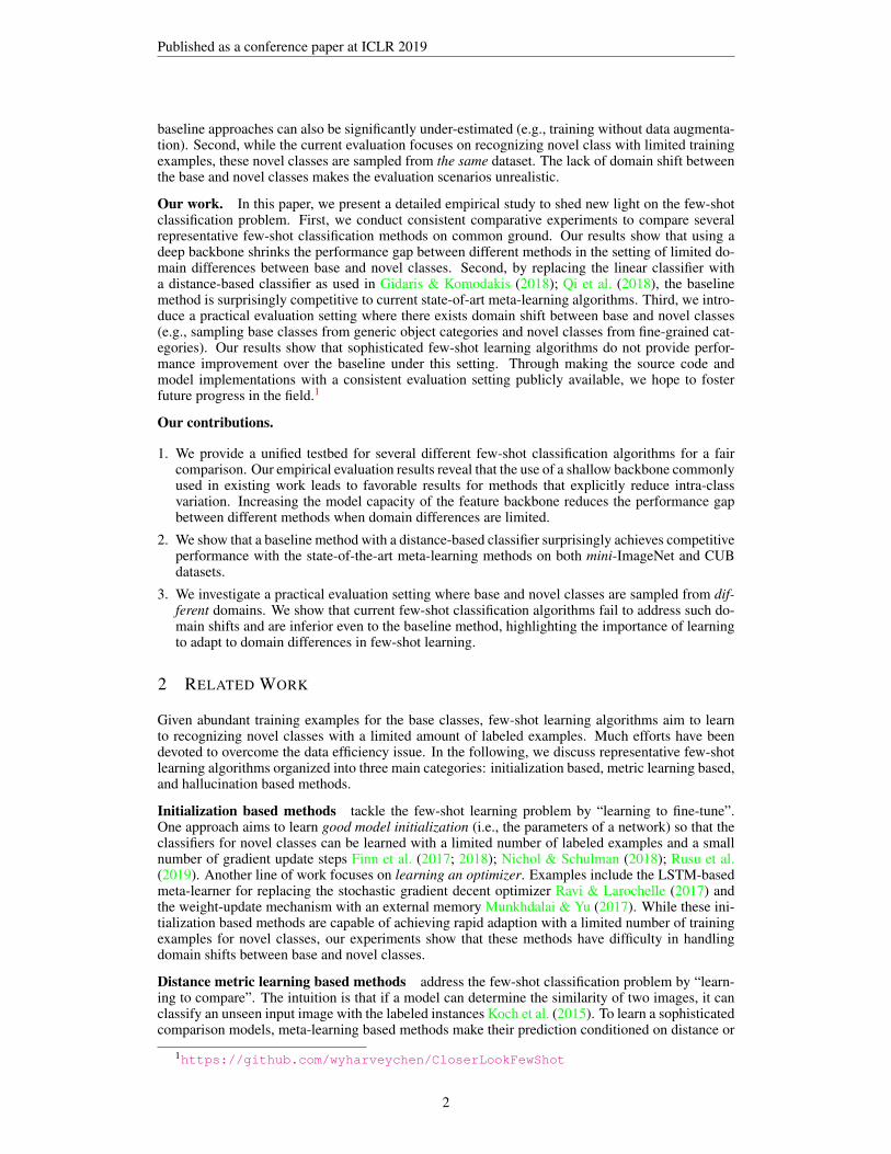
As discussed in Section 4.1, we use first-order approximation MAML to improve memory efficiencyin all of our experiments. To demonstrate this design choice does not affect the accuracy, we comparetheir validation accuracy trends on Omniglot with 5-shot as in Figure A1. We observe that while thefull version MAML converge faster, both versions reach similar accuracy in the end.

This phenomena is consistent with the difference of first-order (e.g. gradient descent) and second-order methods (e.g. Newton) in convex optimization problems. Second-order methods convergefaster at the cost of memory, but they both converge to similar objective value.

Figure A1: Validation accuracy trends of MAML and MAML with first order approximation.Both versions converge to the same validation accuracy. The experimental results are on Omniglotwith 5-shot with a Conv-4 backbone.

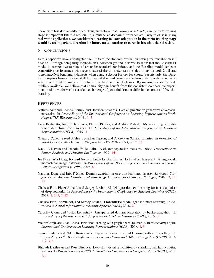
A6 INTRA-CLASS VARIATION AND BACKBONE DEPTH

As mentioned in Section 4.3, here we demonstrate decreased intra-class variation as the networkdepth gets deeper as in Figure A2. We use the Davies-Bouldin index Davies & Bouldin (1979) tomeasure intra-class variation. The Davies-Bouldin index is a metric to evaluate the tightness in acluster (or class, in our case). Our results show that both intra-class variation in the base and novelclass feature decrease using deeper backbones.

2

3

4

5

6

7

8

Conv-4 Conv-6 Resnet-10 Resnet-18 Resnet-343

4

5

6

7


Baseline Baseline++ MatchingNetProtoNet

Base class feature Novel class feature

Dav

ies-

Bou

ldin

inde

x(I

ntra

-cla

ssva

riat

ion)

Figure A2: Intra-class variation decreases as backbone gets deeper. Here we useDavies-Bouldin index to represent intra-class variation, which is a metric to evaluate the tightnessin a cluster (or class, in our case). The statistics are Davies-Bouldin index for all base and novelclass feature (extracted by feature extractor learned after training or meta-training stage) for CUBdataset under different backbone.

14


A7 DETAILED STATISTICS IN EFFECTS OF INCREASING BACKBONE DEPTH

Here we show a high-resolution version of Figure 3 in Figure A3 and show detailed statistics inTable A5 for easier comparison.

45%

55%

65%

75%

40%

45%

50%

55%

60%

70%

80%

90%

60%

65%

70%

75%

80%

Baseline Baseline++ MatchingNet ProtoNet MAML RelationNet

CUB mini-ImageNet

1-sh

ot5-

shot

Figure A3: Few-shot classification accuracy vs. backbone depth. In the CUB dataset, gapsamong different methods diminish as the backbone gets deeper. In mini-ImageNet 5-shot, somemeta-learning methods are even beaten by Baseline with a deeper backbone.

Table A5: Detailed statistics in Figure 3. We put exact value here for reference.


CUB1-shot

Baseline 47.12±0.74 55.77±0.86 63.34±0.91 65.51±0.87 67.96±0.89Baseline++ 60.53±0.83 66.00±0.89 69.55±0.89 67.02±0.90 68.00±0.83

MatchingNet 61.16±0.89 67.16±0.97 71.29±0.90 72.36±0.90 71.44±0.96ProtoNet 51.31±0.91 66.07±0.97 70.13±0.94 71.88±0.91 72.03±0.91MAML 55.92±0.95 65.91±0.97 71.29±0.95 69.96±1.01 67.28±1.08

RelationNet 62.45±0.98 63.11±0.94 68.65±0.91 67.59±1.02 66.20±0.99

CUB5-shot



RelationNet 76.11±0.69 77.81±0.66 81.12±0.63 82.75±0.58 82.30±0.58

mini-ImageNet1-shot



RelationNet 49.31±0.85 51.84±0.88 52.19±0.83 52.48±0.86 51.74±0.83

mini-ImageNet5-shot



RelationNet 66.60±0.69 64.55±0.70 70.20±0.66 69.83±0.68 69.61±0.67

15


A8 MORE-WAY IN META-TESTING STAGE

We experiment with a practical setting that handles different testing scenarios. Specifically, weconduct the experiments of 5-way meta-training and N-way meta-testing (where N = 5, 10, 20) toexamine the effect of testing scenarios that are different from training.

As in Table A6, we compare the methods Baseline, Baseline++, MatchingNet, ProtoNet, and Re-lationNet. Note that we are unable to apply the MAML method as MAML learns the initializationfor the classifier and can thus only be updated to classify the same number of classes. Our resultsshow that for classification with a larger N-way in the meta-testing stage, the proposed Baseline++compares favorably against other methods in both shallow or deeper backbone settings.

We attribute the results to two reasons. First, to perform well in a larger N-way classification setting,one needs to further reduce the intra-class variation to avoid misclassification. Thus, Baseline++ hasbetter performance than Baseline in both backbone settings. Second, as meta-learning algorithmswere trained to perform 5-way classification in the meta-training stage, the performance of thesealgorithms may drop significantly when increasing the N-way in the meta-testing stage because thetasks of 10-way or 20-way classification are harder than that of 5-way one.

One may address this issue by performing a larger N-way classification in the meta-training stage(as suggested in Snell et al. (2017)). However, it may encounter the issue of memory constraint.For example, to perform a 20-way classification with 5 support images and 15 query images in eachclass, we need to fit a batch size of 400 (20 x (5 + 15)) that must fit into the GPUs. Without specialhardware parallelization, the large batch size may prevent us from training models with deeperbackbones such as ResNet.

Table A6: 5-way meta-training and N-way meta-testing experiment. The experimental resultsare on mini-ImageNet with 5-shot. We could see Baseline++ compares favorably against othermethods in both shallow or deeper backbone settings.

Conv-4 ResNet-18N-way test 5-way 10-way 20-way 5-way 10-way 20-way

Baseline 62.53±0.69 46.44±0.41 32.27±0.24 74.27±0.63 55.00±0.46 42.03±0.25Baseline++ 66.43±0.63 52.26±0.40 38.03±0.24 75.68±0.63 63.40±0.44 50.85±0.25

MatchingNet 63.48±0.66 47.61±0.44 33.97±0.24 68.88±0.69 52.27±0.46 36.78±0.25ProtoNet 64.24±0.68 48.77±0.45 34.58±0.23 73.68±0.65 59.22±0.44 44.96±0.26

RelationNet 66.60±0.69 47.77±0.43 33.72±0.22 69.83±0.68 53.88±0.48 39.17±0.25

16

a closer look at few shot classification

Documents