A CLASSIFICATION ALGORITHM USING MAHALANOBIS

DISTANCE CLUSTERING OF DATA WITH APPLICATIONS

ON BIOMEDICAL DATA SETS

A THESIS SUBMITTED TO

THE GRADUATE SCHOOL OF NATURAL AND APPLIED SCIENCES

OF

MIDDLE EAST TECHNICAL UNIVERSITY

BY

BAHADIR DURAK

IN PARTIAL FULFILLMENT OF THE REQUIREMENTS

FOR

THE DEGREE OF MASTER OF SCIENCE

IN

INDUSTRIAL ENGINEERING

JANUARY 2011

Approval of the thesis:

A CLASSIFICATION ALGORITHM USING MAHALANOBIS DISTANCE

CLUSTERING OF DATA WITH APPLICATIONS ON BIOMEDICAL DATA

SETS

submitted by BAHADIR DURAK in partial fulfillment of the requirements for the degree of Master of Science in Industrial Engineering Department, Middle East Technical University by, Prof. Dr. Canan Özgen _____________________ Dean, Graduate School of Natural and Applied Sciences, METU Prof. Dr. Sinan Kayalıgil _____________________ Department Chair, Industrial Engineering Dept., METU Assistant Professor Cem Đyigün _____________________ Supervisor, Industrial Engineering Dept., METU Examining Committee Members: Assoc. Prof. Inci Batmaz, _____________________ Department of Statistics, METU Assistant Professor Cem Đyigün _____________________ Industrial Engineering Dept., METU Assistant Professor Pelin Bayındır _____________________ Industrial Engineering Dept., METU Assistant Professor Serhan Duran _____________________ Industrial Engineering Dept., METU Assistant Prof. Sedef Meral, _____________________ Industrial Engineering Dept., METU

Date: 17.12.2010

iii

I hereby declare that all information in this document has been obtained and

presented in accordance with academic rules and ethical conduct. I also

declare that, as required by these rules and conduct, I have fully cited and

referenced all material and results that are not original to this work.

Bahadır DURAK

iv

ABSTRACT

A CLASSIFICATION ALGORITHM USING MAHALANOBIS DISTANCE

CLUSTERING OF DATA WITH APPLICATIONS ON BIOMEDICAL DATA

SETS

Durak, Bahadır

M.S, Industrial Engineering Department

Supervisor: Assistant Professor Cem Đyigün

January 2011, 91 pages

The concept of classification is used and examined by the scientific community

for hundreds of years. In this historical process, different methods and algorithms

have been developed and used.

Today, although the classification algorithms in literature use different methods,

they are acting on a similar basis. This basis is setting the desired data into classes

by using defined properties, with a different discourse; an effort to establish a

relationship between known features with unknown result. This study was

intended to bring a different perspective to this common basis.

In this study, not only the basic features of data are used, the class of the data is

also included as a parameter. The aim of this method is also using the information

in the algorithm that come from a known value. In other words, the class, in which

the data is included, is evaluated as an input and the data set is transferred to a

higher dimensional space which is a new working environment. In this new

environment it is not a classification problem anymore, but a clustering problem.

Although this logic is similar with Kernel Methods, the methodologies are

different from the way that how they transform the working space. In the

v

projected new space, the clusters based on calculations performed with the

Mahalanobis Distance are evaluated in original space with two different heuristics

which are center-based and KNN-based algorithm. In both heuristics, increase in

classification success rates achieved by this methodology. For center based

algorithm, which is more sensitive to new input parameter, up to 8% of

enhancement is observed.

Keywords: Data Mining, Classification, Clustering, Mahalanobis Distance,

Kernel Function.

vi

ÖZ

BĐOMEDĐKAL VERĐ KÜMELERĐ ÜZERĐNDE MAHALANOBIS UZAKLIĞI

VERĐ KÜMELENMESĐ ĐLE SINIFLANDIRMA ALGORĐTMASI

Durak, Bahadır

Yüksek Lisans, Endüstri Mühendisliği Bölümü

Tez Yöneticisi: Assist. Prof. Cem Đyigün

Ocak 2011, 91 sayfa

Sınıflandırma kavramı bilimsel çevrelerce yüzlerce yıldır kullanılmakta ve

incelenmektedir. Bu tarihsel süreç içerisinde farklı yöntemler ve algoritmalar

geliştirilmiş ve kullanılmıştır.

Bugün literature geçmiş olan sınıflandırma algoritmaları, farklı yöntemler

kullanmakta olsalar da benzer bir temel üzerinde hareket etmektedirler. Bu temel,

tanımlı özellikleri kullanarak, istenen verileri belirlenmiş sınıflarda toplama, farklı

bir söylemle, tanımlanmış nedenler ile sonuç arasında bir ilişki kurabilme

çabasıdır. Bu çalışma, bugüne kadar kullanılmakta olan bu temele farklı bir bakış

açısı getirmeyi amaçlamıştır.

Bu çalışmada, verilerin sadece temel özellikleri değil, sınıfları da bir parametre

olarak kullanılmıştır. Söz konusu yöntemdeki amaç, bilinen bir değerden gelecek

olan bilgiyi de algoritmada kullanma çabasıdır. Diğer bir ifadeyle, verinin dahil

olduğu sınıf, bir girdi olarak değerlendirilmiş ve veri kümesi üst bir uzaya transfer

edilerek yeni bir çalışma ortamı yaratılmıştır. Aynı zamanda bu yeni ortamda artık

problem bir sınıflandırma problemi değil, kümeleme problemidir. Her ne kadar bu

mantık Kernel Yöntemini çağrıştırsa da, yöntemin kullanılış biçimi tamamen

farklıdır. Oluşturulan yeni uzayda Mahalanobis Uzaklığı ile yapılan hesaplamalar

vii

ve oluşturulan kümeler, orijinal uzayda merkez temelli ve KNN temelli 2 farklı

sınıflandırma algoritması ile değerlendirilmiştir. Bu yeni yöntem ile her iki

algoritmada da ulaşılan başarı oranlarında artış yakalanmıştır. Yeni yönteme daha

duyarlı olan merkez temelli algoritma ile başarı oranındaki artışın %8 seviyelerine

kadar çıktığı gözlenmiştir.

Anahtar Kelimeler: Veri Madenciliği, Sınıflandırma, Kümeleme, Mahalanobis,

Kernel.

viii

ACKNOWLEDGMENTS

I would like to thank my supervisor Assist. Prof. Cem Iyigün who guided and

motivated me in this study.

Special thanks are for my family for their patience, love, motivation and

encouragement from the beginning of this long story.

ix

TABLE OF CONTENTS

ABSTRACT ....................................................................................................... iii

ÖZ……... ............................................................................................................ v

LIST OF TABLES ............................................................................................... x

LIST OF FIGURES ............................................................................................ xi

CHAPTERS

1. INTRODUCTION ................................................................................................ 1

2. GENERAL BACKGROUND ............................................................................ 3

2.1. Data ........................................................................................................................ 3

2.2. Data mining ........................................................................................................... 3

2.3. Estimation ............................................................................................................... 4

2.4. Distances ................................................................................................................. 4

2.4.1. Euclidean distance .................................................................... 5

2.4.2. Manhattan distance ................................................................... 5

2.4.3. L∞ norm .................................................................................... 6

2.4.4. Mahalanobis Distance ............................................................... 6

2.5. Learning ................................................................................................................ 10

2.5.1. Supervised Learning ............................................................... 10

2.5.2. Unsupervised Learning ........................................................... 11

2.5.3. Supervised Learning vs. Unsupervised Learning ..................... 11

2.6. Classification Methods .......................................................................................... 12

2.6.1. K-nearest neighbor algorithm ................................................. 13

2.6.2. Neural Networks..................................................................... 14

2.3.3. Support Vector Machine ......................................................... 15

2.3.4. Kernel Methods ...................................................................... 18

2.4. Clustering Methods ............................................................................................... 19

2.4.1. Hierarchical Clustering ........................................................... 20

x

2.4.1.1. Agglomerative Hierarchical Approach ........................ 21

2.4.1.2. Divisive Hierarchical Approach .................................. 24

2.4.2. Center-Based Clustering Algorithms ...................................... 25

2.4.2.1. K-means algorithm ...................................................... 26

2.4.2.2. Fuzzy k-means ............................................................ 28

2.5. Validation .............................................................................................................. 28

2.5.1. K fold cross validation ............................................................ 29

2.5.2. Type-I and Type-II Error ........................................................ 31

3. METHODOLOGY ............................................................................................. 32

3.1. Terminology ............................................................................................................... 32

3.2. Effect of α and Geometrical Interpretation ................................................................ 36

3.3. Center Based Algorithm............................................................................................. 38

3.4. KNN Based Algorithm .............................................................................................. 40

4. APPLICATION .................................................................................................. 42

5. DISCUSSIONS AND EVALUATIONS ........................................................ 45

6. CONCLUSION AND FURTHER STUDIES ................................................ 49

REFERENCES .................................................................................................. 51

APPENDICES ................................................................................................... 55

Appendix A – Algorithms in MATLAB ..................................................................... 55

Appendix B – Source Code for Data set Generation ................................................ 74

Appendix C – Application in MATLAB..................................................................... 76

C.1. Center Based Algorithm ........................................................................................... 76

C.2. KNN Based Algorithm ............................................................................................. 84

C.3. Center Based Algorithm Results on Biomedical Data sets ...................................... 85

C.4. KNN Based Algorithm Results on Biomedical Data sets ........................................ 91

xi

LIST OF TABLES

TABLE 2.1- SUPERVISED LEARNING VS. UNSUPERVISED LEARNING . 11

TABLE 3.1- THE MEANINGS OF X-SPACE AND Y-SPACE ........................ 32

TABLE 4.1- PROPERTIES OF BIOMEDICAL DATA SETS........................... 43

TABLE 4.2- EXECUTION TIMES WITH BIOMEDICAL DATA SETS .......... 44

TABLE 5.1- ENHANCEMENT IN CENTER BASED HEURISTIC BY � WITH

BIOMEDICAL DATA SETS ..................................................................... 48

TABLE 5.2- ENHANCEMENT IN KNN BASED HEURISTIC BY � WITH

BIOMEDICAL DATA SETS ..................................................................... 48

xii

LIST OF FIGURES

FIGURE 2-1 - GENERATED DATA AND SELECTED POINTS A, B .............. 8

FIGURE 2-2 - GENERATED DATA AND SELECTED POINTS C, D .............. 9

FIGURE 2-3 - CLASSIFICATION PROCESS .................................................. 12

FIGURE 2-4 - GEOMETRICAL REPRESENTATION OF K-NEAREST

NEIGHBOR ALGORITHM ................................................................... 14

FIGURE 2-5 - THE BASIC ARCHITECTURE OF THE FEED FORWARD NEURAL NETWORK ........................................................................... 15

FIGURE 2-6 - PRINCIPLE OF SUPPORT VECTOR MACHINE ..................... 17

FIGURE 2-7 - MATHEMATICAL EXPRESSIONS OF SUPPORT VECTOR MACHINE ............................................................................................. 18

FIGURE 2-8 - PRINCIPLE OF KERNEL METHODS ...................................... 19

FIGURE 2-9 - SAMPLE DENDOGRAM .......................................................... 21

FIGURE 2-10 - K-FOLD CROSS VALIDATION PROCESS ......................... 30

FIGURE 3-1 - SEPARABLE CASE .................................................................. 34

FIGURE 3-2 - HALF - SEPARABLE CASE ..................................................... 35

FIGURE 3-3 - NOT-SEPARABLE CASE ......................................................... 36

FIGURE 3-4 - EFFECT OF � TO EXAMPLE 1 (SEPARABLE CASE) ........... 37

FIGURE 3-5 - EFFECT OF � TO EXAMPLE 2 (HALF-SEPARABLE CASE) 37

FIGURE 3-6 - EFFECT OF � TO EXAMPLE 3 (NOT-SEPARABLE CASE) .. 38

FIGURE 4-1 - CLASSIFICATION SUCCESS RATES OF CENTER BASED HEURISTIC WITH EUCLIDEAN DISTANCE ..................................... 42

FIGURE 5-1 - CLASSIFICATION SUCCESS RATES OF WINE DATA SET

(CENTER BASED HEURISTIC WITH MAHALANOBIS DISTANCE) ............................................................................................................... 45

FIGURE C-1- SUCCESS RATE VS. VALUE, CENTER BASED

ALGORITHM WITH EUCLIDEAN DISTANCE SUCCESS RATE OF

SEPARATED, EUCLIDEAN, K=2 ........................................................ 76

FIGURE C-2- SUCCESS RATE VS. VALUE, CENTER BASED ALGORITHM WITH MAHALANOBIS DĐSTANCE .......................... 77

xiii

FIGURE C-3- SUCCESS RATE VS. NUMBER OF CLUSTERS, CENTER

BASED ALGORITHM ON SEPARATED DATA WITH EUCLIDEAN

DISTANCE ........................................................................................... 78

FIGURE C-4- SUCCESS RATE VS. NUMBER OF CLUSTERS, CENTER

BASED ALGORITHM ON HALF-SEPARATED DATA WITH EUCLIDEAN DISTANCE .................................................................... 79

FIGURE C-5- SUCCESS RATE VS. NUMBER OF CLUSTERS, CENTER

BASED ALGORITHM ON NOT-SEPARATED DATA WITH

EUCLIDEAN DISTANCE .................................................................... 80

FIGURE C-6- SUCCESS RATE VS. NUMBER OF CLUSTERS, CENTER

BASED ALGORITHM ON SEPARATED DATA WITH

MAHALANOBIS DISTANCE ............................................................. 81

FIGURE C-7- SUCCESS RATE VS. NUMBER OF CLUSTERS, CENTER

BASED ALGORITHM ON HALF-SEPARATED DATA WITH MAHALANOBIS DISTANCE ............................................................. 82

FIGURE C-8- SUCCESS RATE VS. NUMBER OF CLUSTERS, CENTER

BASED ALGORITHM ON NOT-SEPARATED DATA WITH MAHALANOBIS DISTANCE ............................................................. 83

FIGURE C-9- SUCCESS RATE VS. � VALUE, KNN BASED ALGORITHM

............................................................................................................... 84

FIGURE C-10- SUCCESS RATE OF DIABETIS DATA SET, CENTER BASED ALGORITHM WITH MAHALANOBIS DISTANCE ......................... 85

FIGURE C-11- SUCCESS RATE OF HEPAITIS DATA SET, CENTER BASED ALGORITHM WITH MAHALANOBIS DISTANCE ......................... 86

FIGURE C-12- SUCCESS RATE OF LIVER CANCER DATA SET, CENTER

BASED ALGORITHM WITH MAHALANOBIS DISTANCE ............ 87

FIGURE C-13- SUCCESS RATE OF VOTING DATA SET, CENTER BASED ALGORITHM WITH MAHALANOBIS DISTANCE ......................... 88

FIGURE C-14- SUCCESS RATE OF WINE DATA SET, CENTER BASED ALGORITHM WITH MAHALANOBIS DISTANCE ......................... 89

FIGURE C-15- SUCCESS RATE OF BREAST CANCER DATA SET, CENTER BASED ALGORITHM WITH MAHALANOBIS DISTANCE ............ 90

FIGURE C-16- SUCCESS RATE OF BIOMEDICAL DATA SETS, KNN

BASED ALGORITHM WITH MAHALANOBIS DISTANCE ............ 91

1

CHAPTER 1

INTRODUCTION

Various classification approaches try to find a function that estimates the class

labels from the feature-space in a data set. In these methodologies, named

“supervised learning”, the features are accepted as input while the class labels are

accepted as output. On the other hand, in the clustering approaches (unsupervised

learning) there are no class labels. Instead, they try to create groups according to

similarities of the data points. In this approach there is no class information and

only feature space is used in clustering process.

Both classification and clustering approaches do not use the information from

class labels as a parameter in the process. This study searches a methodology

which takes this information into consideration. There are two new heuristics

developed in which the information from the class is integrated: Center based

algorithm and KNN based algorithm.

In center based heuristic, information from the class labels is included to feature

space in training stage. By this, the dimension of feature space increases by one

and the problem becomes a clustering problem. There are two important processes

which are hidden in this methodology. First, data points are mapped to a high

dimensional space, so that kernel logic is used in this methodology. Second the

classification problem turns into a clustering problem, such that the original

problem is transformed into a new clustering problem.

In KNN based heuristic the class information is included in feature space similar

with center based heuristic. The difference is the algorithm keeps this information

as class information, too. There is also kernel logic since the original problem

mapped to a high dimensional space, but the original problem is still a

classification problem.

2

This new methodology arises new questions. One of these questions is how to

weight the information from the class labels, which is a new parameter, to

produce better classification results. The label information can have equal effect

or the feature can have higher effect with different weights. In order to find the

effects of new parameter, a compound distance is generated unifying the distance

in the feature space and class labels. This approach is explained and studied in this

thesis.

Other question is which distance measure should be used as a basis of this new

distance function. The distance measure may differ in various classification

problems, the content and the application area mostly determines the selection of

the distance function used. The data types and the relationships between them

determine the type of the distance measure. For example, in biomedical data sets

there are some correlations within the features (variables). In this study the data

sets are numerical and to take into account the correlations, Mahalanobis

Distance is chosen. In order to measure the effect of this choice, Euclidean

distance is also used to compare the results. If the variables are not numeric

(which is common in biological and biomedical data sets), then a suitable

distance, i.e. hamming distance, need to be used.

Another question is how the other parameters affect the classification success rate.

The effect of number of clusters in center based algorithm and number of

neighbours in KNN based algorithm are investigated. The effects of these

parameters are explained and illustrated in the study.

3

CHAPTER 2

GENERAL BACKGROUND

2.1. Data

Observations (data points) are the objects of data mining. Data points are consist

of different attributes which are in an order. A data point x with m attributes is an

m-dimensional vector, x = (x1, x2, ... , xm). N data points xi form a set

� = ���, ��, … , � ⊂ ℝ� (1.1)

Called the data set. � can be represented by an N × m matrix

� = ����� (1.2)

where ��� is the ��� component of the data point xi.

2.2.Data mining

Generally speaking, data mining is the process of extracting or ‘mining’ implicit

and relevant information from large sets of data. A more precise definition of the

term would be “the non trivial extraction of implicit, previously unknown, and

potentially useful knowledge from large volumes of actual data” (Piateski &

Frawley, 1991, cited by Lee & Kim, 2002, pp. 42) Data mining is also known by

several other terms depending on the situation and context, such as knowledge

mining from data, knowledge extraction, data/pattern analysis, data archaeology,

and data dredging. The primary aim of data mining is to gather sense, or extract

predictive information, from large amounts of mostly unsupervised data, in a

particular domain. The largest group of data mining users is businesses, since

collecting large amount of data and making sense out of it happens to be one of

their routine activities. (Cios et. al., 2007, pp. 3-4)

4

2.3.Estimation

Estimating outputs based on input variables is one of the most important problems

in empirical research. The meaning of estimation is the calculated approximation

of a result when there is an uncertainty in finding the output or the inputs are not

known exactly. In a wide range of engineering areas, estimation techniques are

used. Aerospace systems, communications, manufacturing and biomedical

engineering are the areas that estimation techniques are mostly used. The

estimation of the health of a person’s hearth based on an electrocardiogram (ECG)

is a specific example of usage in biomedical engineering (Kamen & Su, 1999, pp.

1).

2.4.Distances

There are several techniques used for data mining. Several such techniques, for

instance nearest neighbor classification methods, cluster analysis, and

multidimensional scaling methods, are based on the measures of similarity

between objects. Instead of measuring similarity, dissimilarity between the objects

too will give the same results. For measuring dissimilarity one of the parameters

that can be used is distance. This category of measures is also known as

separability, divergence or discrimination measures. (Hand, Mannila, & Smyth,

2001, pp. 31) A distance metric is a real-valued function d, such that for any

points x, y, and z:

���, � ≥ 0 , and ��, � = 0 , if and only if � = � (2.1)

���, � = ���, � (2.2)

���, � ≤ ���, � + ���, � (2.3)

The first property, positive definiteness, assures that distance is always a non-

negative quantity, so the only way distance can be zero is for the points to be the

same. The second property indicates the symmetry nature of distance. The third

5

property is the triangle inequality, according to which introducing a third point

can never shorten the distance between two points. (Larose, 2005, pp. 99) There

are several measures of distance which satisfy the metric properties, some of

which are discussed below:

2.4.1. Euclidean distance

The Euclidean distance is the most common distance metric used in low

dimensional data sets. It is also known as the L2 norm. The Euclidean distance is

the usual manner in which distance is measured in real world. In this sense,

Manhattan distance tends to be more robust to noisy data.

�� !"�#�$%��, � = &∑ ��� − )��� (2.4)

where x and y are m-dimensional vectors and denoted by x = (x1, x2, x3... xm) and

y = (y1, y2, y3... ym) represent the m attribute values of two records. (Larose, 2005,

pp. 99) While Euclidean metric is useful in low dimensions, it doesn’t work well

in high dimensions and for categorical variables. The drawback of Euclidean

distance is that it ignores the similarity between attributes. Each attribute is treated

as totally different from all of the attributes. (Ertöz, Steinbach & Kumar, 2003, pp.

49)

2.4.2. Manhattan distance

This metric is also known as the L1 norm or the rectilinear distance. This is also

a common distance metric and gets its name from the rectangular grid patterns of

streets in midtown Manhattan. Hence, another name for the distance metric is also

city block distance. It is defined as the sum of distances travelled along each axis.

The Manhattan distance looks at the absolute differences between coordinates. In

some situations, this metric is more preferable to Euclidean distance, because the

distance along each axis is not squared so a large difference in one dimension will

not dominate the total distance. (Berry & Linoff, 2009: 363)

�*$%�$��$%��, � = ∑ |�� − )�|��,� (2.5)

6

2.4.3. L∞ norm

The L∞ norm is the maximum of the absolute differences in any single dimension.

It is also known as sup norm or the maximum norm. Another name for L∞ norm

is Chebyshev norm. Chebyshev norm is also called as chessboard distance;

since it is equal to the number of moves it takes a chess king to occupy any other

point on the chessboard. This distance metric looks only at the measurement on

which attributes deviates the most. Chebyshev distances are piecewise linear. In

fact, like the Manhattan distance, the Chebyshev distance examines the absolute

magnitude of the element-wise differences between the attributes. (Bock &

Krischer, 1998, pp. 13)

�-.��, � = max�,�,�,…,�|�� −)�| (2.6)

2.4.4. Mahalanobis Distance

Mahalanobis distance is a well known statistical distance function. Here, a

measure of variability can be incorporated into the distance metric directly.

Mahalanobis distance is a distance measure between two points in the space

defined by two or more correlated variables. That is to say, Mahalanobis distance

takes the correlations within a data set between the variable into consideration. If

there are two non-correlated variables, the Mahalanobis distance between the

points of the variable in a 2D scatter plot is same as Euclidean distance. In

mathematical terms, the Mahalanobis distance is equal to the Euclidean distance

when the covariance matrix is the unit matrix. This is exactly the case then if the

two columns of the standardized data matrix are orthogonal. The Mahalanobis

distance depends on the covariance matrix of the attribute and adequately

accounts for the correlations. Here, the covariance matrix is utilized to correct the

effects of cross-covariance between two components of random variable. (Hill &

Lewicki, 2006, pp. 164)

7

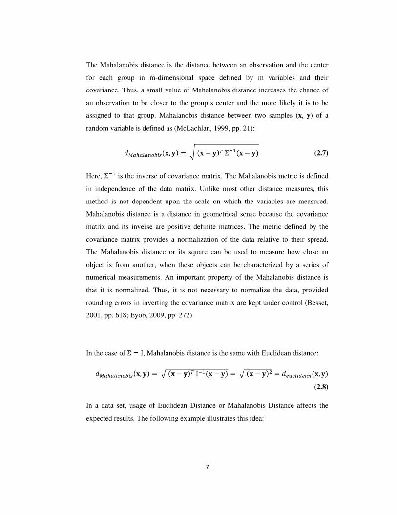
The Mahalanobis distance is the distance between an observation and the center

for each group in m-dimensional space defined by m variables and their

covariance. Thus, a small value of Mahalanobis distance increases the chance of

an observation to be closer to the group’s center and the more likely it is to be

assigned to that group. Mahalanobis distance between two samples (x, y) of a

random variable is defined as (McLachlan, 1999, pp. 21):

�*$�$"$%23�4��, � = 5�� − �6Σ7��� − � (2.7)

Here, Σ7� is the inverse of covariance matrix. The Mahalanobis metric is defined

in independence of the data matrix. Unlike most other distance measures, this

method is not dependent upon the scale on which the variables are measured.

Mahalanobis distance is a distance in geometrical sense because the covariance

matrix and its inverse are positive definite matrices. The metric defined by the

covariance matrix provides a normalization of the data relative to their spread.

The Mahalanobis distance or its square can be used to measure how close an

object is from another, when these objects can be characterized by a series of

numerical measurements. An important property of the Mahalanobis distance is

that it is normalized. Thus, it is not necessary to normalize the data, provided

rounding errors in inverting the covariance matrix are kept under control (Besset,

2001, pp. 618; Eyob, 2009, pp. 272)

In the case of Σ = Ι, Mahalanobis distance is the same with Euclidean distance:

�*$�$"$%23�4��, � = &�� − �6I7��� − � = &�� − �� = �� !"�#�$%��, � (2.8)

In a data set, usage of Euclidean Distance or Mahalanobis Distance affects the

expected results. The following example illustrates this idea:

8

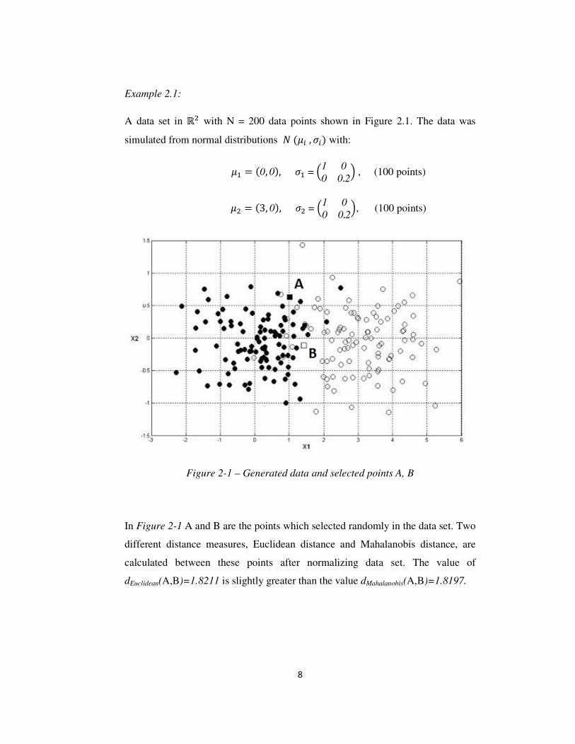
Example 2.1:

A data set in ℝ� with N = 200 data points shown in Figure 2.1. The data was

simulated from normal distributions ;�<�, =� with:

<� = �0, 0,=� = >1 0

0 0.2@ , (100 points)

<� = �3, 0,=� = >1 0

0 0.2@, (100 points)

Figure 2-1 – Generated data and selected points A, B

In Figure 2-1 A and B are the points which selected randomly in the data set. Two

different distance measures, Euclidean distance and Mahalanobis distance, are

calculated between these points after normalizing data set. The value of

dEuclidean(A,B)=1.8211 is slightly greater than the value dMahalanobis(A,B)=1.8197.

9

Example 2.2:

A data set in ℝ�with N = 200 data points shown in Figure 2-1. The data was

simulated from normal distributions ;�<�, =� with:

<� = �0, 0,=� = >1 0

0 0.2@ , (100 points)

<� = �6, 0,=� = >1 00 0.2@, (100 points)

Figure 2-2 – Generated data and selected points C, D

In Figure 2-2 C and D are the points which selected randomly in the data set.

Same with example 2.1, two different distance measures, Euclidean distance and

Mahalanobis distance, are calculated between these points after normalizing data

set. Contrary to example 2.1, the value of dEuclidean(C,D) = 1.9099 is now smaller

than the value dMahalanobis(C,D) = 7.7996.

10

So, it can be seen from the results of examples 2.1 and 2.2 that:

�E !"�#�$%�A, B > �*$�$"$%23�4�A, B (2.9)

But on the contrary,

�E !"�#�$%�C, D < �*$�$"$%23�4�C, D (2.10)

It illustrates the effect of covariance matrix Σ on the distance. Depending on the

structure of the data, Σ can produce a shorter distance or longer distance than

Euclidean Distance.

2.5. Learning

The term learning refers acquiring knowledge from a set of data or briefly

understanding the data. The learning process is executed in a partition of the

original set which is called training set. Since training sets are finite and the future

is not certain, the performance of the learning process should be measured. This

can be done by using test set, another partition of original data set. In the area of

data mining, learning techniques are classified in two classes:

2.5.1. Supervised Learning

This is also known as directed data mining. In supervised learning the variables

that are under investigation are first separated into two groups: input variables,

and one output variable or more than one output variables (labels). (Taylor &

Agah, 2008, pp. 50) Pre-classification is a prerequisite for supervised learning.

That is to say, the variables in the data set need to be already placed in groups or

assigned some value or result. (Shmueli et. al., 2008, pp. 11) Supervised learning

is predictive in nature i.e. data is learnt with an answer. The aim of the data

mining exercise is to find a relationship between these two types of variables. An

important requirement for supervised learning is that the values of the output

variable (label) must be known for a sufficiently large part of the data set.

(Wübben, 2008, pp. 137)

11

2.5.2. Unsupervised Learning

Unlike for supervised learning, unsupervised learning does not require the target

variable to be well defined and that a sufficiently large number of values are

known. In case of unsupervised learning, the target variable is unknown. (Taylor

& Agah, 2008, pp. 50) Unsupervised learning occurs when the data is not

previously classified. Here, the data mining process cannot take value decisions.

The data mining process can find correlations within data, but cannot make any

inferences on what the patterns mean. (Shmueli et. al., 2008, pp. 11)

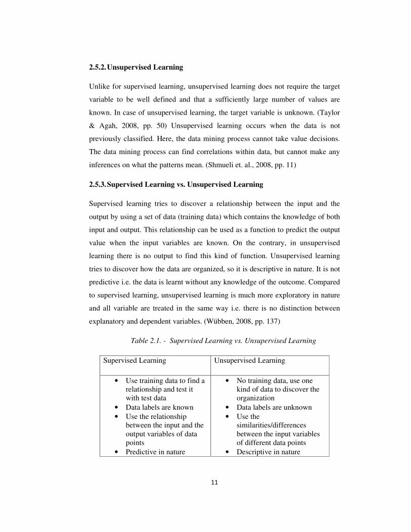
2.5.3. Supervised Learning vs. Unsupervised Learning

Supervised learning tries to discover a relationship between the input and the

output by using a set of data (training data) which contains the knowledge of both

input and output. This relationship can be used as a function to predict the output

value when the input variables are known. On the contrary, in unsupervised

learning there is no output to find this kind of function. Unsupervised learning

tries to discover how the data are organized, so it is descriptive in nature. It is not

predictive i.e. the data is learnt without any knowledge of the outcome. Compared

to supervised learning, unsupervised learning is much more exploratory in nature

and all variable are treated in the same way i.e. there is no distinction between

explanatory and dependent variables. (Wübben, 2008, pp. 137)

Table 2.1. - Supervised Learning vs. Unsupervised Learning

Supervised Learning Unsupervised Learning

• Use training data to find a

relationship and test it

with test data

• Data labels are known

• Use the relationship

between the input and the

output variables of data

points

• Predictive in nature

• No training data, use one

kind of data to discover the

organization

• Data labels are unknown

• Use the

similarities/differences

between the input variables

of different data points

• Descriptive in nature

12

2.6. Classification Methods

One of the most commonly applied data mining methods is classification. It is a

form of predictive modeling and defines groups within the population. The

process of classification aims to find a model or function describing and

distinguishing data classes or concepts. The aim of classification is to use the

derived function to predict label of data points with unknown class labels. Using

classification method, one can learn functions or rules that form categories of

data. (Han & Kamber, 2006, pp. 24) The functions or rules are derived by an

analysis of a set of data objects with known labels which can be called as training

data. The process of classification has several applications in varied fields such as

medicine, credit card portfolio and credit ranking, customer purchase behavior,

and strategic management. (Li and Shi, 2005, pp. 758)

For classification task, input data is a collection of observations. Each

observation, also known as example or instance, is denoted by (x, y), where x is

the vector of attributes and y is the class label or category of the observation.

Classification is the process of learning a function f that matches each attribute

vector x with one of previously defined class labels y. This process is shown

simply in the Figure 2-3.

Input Output

Attribute vector

(x)

Class Label

(y)

Figure 2-3 – Classification Process

The probability of a class membership can be predicted by classification models

which use the information gathered from input variables. The process of

Classification

Model

13

classification is done in two steps. First, a model is built which describes a

previously determined set of data classes or concepts; second, the model is used

for classification. The first step is known as training phase, where algorithms are

used to learn models to fit training data. The second step is known as testing phase

where testing data is used on obtained models to measure learning success by

predicting class labels of this data set. (Leondes, 2005, pp. 117) From the

description of the process above, two main goals of the classification process can

be gleaned: an accurate model, which can be used in the prediction; and an

explanation of the models itself i.e. a comprehensible explanation for human

experts. Classification focuses primarily on inclusion or exclusion in small set of

specific categories. In case of classification in data mining, the focus is less on

model assumptions and more on the model’s ability to actually predict outcomes.

The classification methods used in data mining are similar, if not identical, to

those used for statistical inference. These methods are explained in the following

sections in an order of increasing complexity. (Cerrito, 2007, pp. 242-243)

2.6.1. K-nearest neighbor algorithm

The K-nearest neighbor algorithm (KNN) is one of the basic and common

classification algorithms. No pre-processing of labeled data samples is needed

before using this algorithm. A dominated class label in K-nearest neighbors of a

data point is assigned as class label to that data point. A tie occurs when

neighborhood has same amount of labels from multiple classes. To break the tie,

the distances of neighbors can be summed up in each class that is tied and vector f

is assigned to the class with minimal distance. Or, the class can be chosen with the

nearest neighbor. Clearly, tie is still possible here, in which case an arbitrary

assignment is taken.

The KNN algorithm is very easy to implement. It performs well in practice

provided that the different attributes or dimensions are normalized, and that the

attributes are independent of one another and relevant to the prediction task at

hand. The main drawback of the KNN algorithm is that each of the K-nearest

14

neighbors is equally important. However, it is obvious that the closer a neighbor

is, the more is the possibility of having the vector f in the class of this neighbor.

Hence, it is better to assign the neighbors with different voting weights based on

their distance with the vector f. (Thuraisingham, et. al., 2009, pp. 196)

Figure 2-4- Geometrical representation of k-nearest neighbor algorithm

2.6.2. Neural Networks

A neural network, when used for classification, is typically a collection of neuron-

like processing units with weighted connections between the units. Artificial

neural networks (ANN) are simple computer programs which can automatically

find relationships in data without any predefined model. ANNs are highly

parameterized nonlinear statistical models. An ANN transforms a real-valued

vector in the input space to a real-valued vector in some output space. They can be

used to predict new characteristics e.g. class membership of points in the input

space. ANNs first linearly transform the input vector by multiplying it with a

weight matrix (Weight matrix = [L��] in Figure 2-4). Then, a nonlinear function is

applied to each coordinate of the resulting vector to produce a value. An

activation function (g in Figure 2-4) produces the output by comparing this value

with threshold (t in Figure 2-4). This is an example of a single layer network. A

multilayer network can be constructed by subsequent application to another

weight matrix and a nonlinear transformation. Training an ANN involves

determining the weight matrix that minimizes the prediction error for a set of

15

training data for which there is knowledge of what the output vector should be.

(Han and Kamber, 2006, pp. 327; Maimon and Rokach, 2005, pp. 488)

The most common application of neural network is to train it on historical data

and then use this model to predict the outcome for new combinations of inputs.

The network possibly extracts a general relationship which holds for all

combination of inputs. In classification problems, the output will have one of two

values, representing belongs to the set and does not belong to the set, whereas in

regression problems the output is a continuous variable. Neural networks do not

give an exact physical model but learn to represent the relationship in terms of the

activation functions of the neurons. (Maimon and Rokach, 2005, pp. 488)

Figure 2-5 - The basic architecture of the feed forward neural network

2.3.3. Support Vector Machine

Support Vector Machines (SVMs) are one of the most recent additions to machine

learning algorithms. Basically, the SVM is binary learning with some highly

elegant property. They calculate a hyperplane between that separates two different

16

classes in the training set. Each object can be transformed as another point in a

high-dimensional space. Sometimes it is not possible to separate the points of two

different classes by a hyperplane in the original space. That is why a

transformation may be needed. Transformed points may be separated by a

hyperplane in a high-dimensional space. These kind of transformations may not

be so easy. In SVM, the kernel is introduced so that computing the hyperplane

becomes very fast. (Hearst, 1998, pp. 19)

Support vectors are the data vectors with shortest distance to the separating

hyperplane. Vectors are simply those data points (for the linearly separable case)

that are the most difficult to classify and optimally separated from each other.

That’s why the hyperplane which has maximum margin is the best separator. In a

support vector machine, the selection of basis function is required to satisfy

Mercer’s theorem; that is, each basis function is in the form of a positive definite

inner-product kernel:

M��N, �O� = P��N ∙ P��O (2.11)

Here, xi, xj are input vectors examples i and j, and φ is the vector of hidden-unit

outputs for inputs xj. The hidden (feature) space is chosen as a high dimensional

space, since transformation of the problem from a nonlinear separable

classification to a linear separable classification becomes possible. The above

condition is also known as the kernel trick. When there are K>2 classes, SVMs

can be used to build K hyperplanes each separating one class from the union of all

other classes. Classification of a test data point starts with computing its distance

to each of the K hyperplanes. The data point is assigned to the class for which this

distance is maximal. (Zhang et. al., 2005, pp. 62)

SVM is currently the best of all classification techniques available. SVMs are

usually considered to be non-parametric models, not because they do not have any

parameters, but because these parameters are not previously defined and their

number depends on the training data used. The only drawback of SVM is the

complexity of training. The SVM also faces problems due to optimization, but this

17

is solved in a dual formulation which makes its size dependent on the number of

the support vectors and not on the dimensionality of the input space. This allows

the use of kernel functions in the linearly separable case without increasing the

algorithmic complexity of the method. These advantages coupled with the sound

and well developed theoretical foundations in mathematical optimizations make

SVM one of the most widely implemented classification methods. (Gallus, et. al.

2008, pp. 62)

• Possible hyperplanes that

separate data

The hyperplane that has maximum

margin is the best separator

Figure 2-6 - Principle of Support Vector Machine

18

Figure 2-7 - Mathematical Expressions of Support Vector Machine

2.3.4. Kernel Methods

Most of the methods usually consider classification as a linear function of the

training data or a hyperplane that can be defined by a set of linear equations on the

training data. However, it is also possible that there exists no hyperplane to

separate the data. As an alternative, a way to build a nonlinear decision surface

can also be a solution. An extremely useful generalization that can give nonlinear

surfaces and improved separation of data are possible. The solution given was by

means of a Kernel Transformation. The Kernel method is to note that there are

classes of function Ф that satisfy the special property of a kernel function K

where,

M��N, �O� = P��N ∙ P��O (2.11)

Then everywhere that �N ∙ �O occurs, it is replaced by M��N, �O�. It is not necessary

to compute P�� explicitly. Only Kernel functions need to be computed. In fact,

an explicit representation of P is not necessary at all, only K is required. A

function can be defined as a Kernel function if it satisfies Mercer’s condition.

(Camps-Valls and Bruzzone, 2009, pp. 66-67)

19

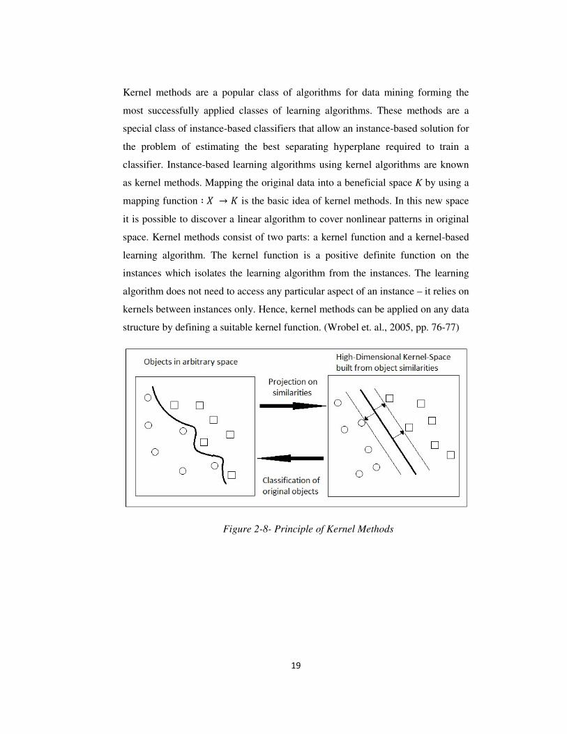
Kernel methods are a popular class of algorithms for data mining forming the

most successfully applied classes of learning algorithms. These methods are a

special class of instance-based classifiers that allow an instance-based solution for

the problem of estimating the best separating hyperplane required to train a

classifier. Instance-based learning algorithms using kernel algorithms are known

as kernel methods. Mapping the original data into a beneficial space K by using a

mapping function ∶ S → M is the basic idea of kernel methods. In this new space

it is possible to discover a linear algorithm to cover nonlinear patterns in original

space. Kernel methods consist of two parts: a kernel function and a kernel-based

learning algorithm. The kernel function is a positive definite function on the

instances which isolates the learning algorithm from the instances. The learning

algorithm does not need to access any particular aspect of an instance – it relies on

kernels between instances only. Hence, kernel methods can be applied on any data

structure by defining a suitable kernel function. (Wrobel et. al., 2005, pp. 76-77)

Figure 2-8- Principle of Kernel Methods

20

2.4. Clustering Methods

Clustering arises as an algorithmic framework for data mining. It is an important

task in several data mining applications including document retrieval and image

segmentation. The word clustering is a kind of decomposition of a set of data

points into natural groups. In other words, it is process of finding and describing

cluster i.e. homogenous groups of entities, in data sets. There are two aspects to

this task: the first involves algorithmic issues on how to find such decompositions

i.e. tractability, while the second concerns quality assignment, i.e. how good is the

computer decomposition. Clustering was originally introduced to the data mining

research as the unsupervised classification of patterns into groups. Clustering

techniques help us to form groups that are internally dense and that are similar

with each other. (Rastegar et. al., 2005, pp. 144)

Clustering needs two basic processes. First one is the creation of a similarity

matrix or distance matrix. A number of techniques can be used to calculate the

distance metric such as Euclidean distance or the use of a standard correlation

coefficient.

2.4.1. Hierarchical Clustering

Hierarchical clustering is a methodology to form good clusters in the data set

using a computationally efficient technique. This type of method allows a user to

ascertain for a comprehensible solution without having to investigate all possible

arrangements. Hierarchical clustering algorithms include a consecutive process and

are a type of unsupervised learning. Algorithms are found to figure out how to

cluster an unordered set of input data without ever being given any training data

with the correct answer. As the name implies, the output of a hierarchical

clustering algorithm is a bunch of fully nested sets. The smallest sets are the

individual sets while the largest is the whole data set. (Minh, et. al, 2006, pp. 160)

After hierarchical clustering is completed, the results are usually viewed in a type

of graph called dendogram, which displays the nodes arranged into their

21

hierarchy. A dendogram not only uses connections to show which items ended up

in each cluster, it also shows how far apart the items were. Figure 2-9 below

shows a sample dendogram. From the figure, it is clear that the EF cluster is a lot

closer to the individual E and F items than the BC cluster is to the individual B

and C items. Rendering the graph this way can help to determine how similar the

items within a cluster are, which could be interpreted as the tightness of the

cluster.

Figure 2-9- Sample Dendogram

Hierarchical clustering techniques can be classified into the following two types

(In practice, both approaches often result in similar trees):

2.4.1.1. Agglomerative Hierarchical Approach

This approach is bottom-up and consists of clumping. In each step of the

agglomerative hierarchical approach, a new cluster is formed by merging an

observation into a previously defined cluster. This process is irreversible; in other

words, any two items merged into a cluster cannot be separated in any following

steps. The relationship between the two items joined is defined by a metric such

as the Euclidean distance. In this process, the clusters grow larger while the

number of cluster shrinks. If one starts with n clusters i.e. individual items, they

end with one single cluster containing the entire data set. A clustering tree is

defined by the path taken to achieve the structure. Agglomerative techniques

conduce to give more precision at the bottom of a tree. Agglomerative approach is

the more preferred choice. As the process of hierarchical method is irreversible,

an optional approach is to carry a hierarchical procedure followed by a

22

partitioning procedure in which items can be moved from one cluster to another.

(Pedrycz, 2005, pp. 6) The number of ways of partitioning a set of n items into k

clusters is given by

;�U, V = �W! ∑ �VY�−1W7�Y%W�,� (2.12)

Algorithms that are representative of the agglomerative clustering approach

include the ones given below. The algorithms differ from each other in terms of

their definition of the distances between two clusters. The closest clusters or the

clusters with the smallest distance between them are merged (Seber, 2004, pp.

359).

Algorithm 2.1 - Agglomerative Hierarchical Approach Algorithm

Step 0. Begin with the disjoint clustering having level L(0) = 0 and

sequence number m = 0

Step 1. Find the least dissimilar pair of clusters, say pair (r), (s):

d[(r),(s)] = min d[(i),(j)] for all pairs i ,j where i ≠ j.

Step 2. Update m :=m +1. Merge clusters (r) and (s) into a single

cluster, Set the level of this clustering to L(m) = d[(r),(s)]

Step 3. Update the proximity matrix by deleting the rows and columns

corresponding to clusters (r) and (s) and adding a row and

column corresponding to the newly formed cluster.

Step 4. If all objects are in one cluster, stop. Else, go to step 1.

23

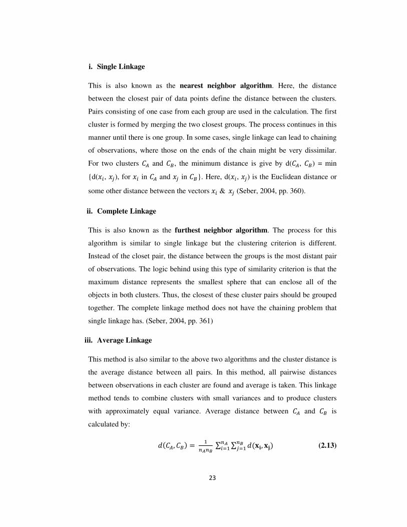
i. Single Linkage

This is also known as the nearest neighbor algorithm. Here, the distance

between the closest pair of data points define the distance between the clusters.

Pairs consisting of one case from each group are used in the calculation. The first

cluster is formed by merging the two closest groups. The process continues in this

manner until there is one group. In some cases, single linkage can lead to chaining

of observations, where those on the ends of the chain might be very dissimilar.

For two clusters Z[ and Z\, the minimum distance is give by d(Z[, Z\) = min

{d(��, ��), for �� in Z[ and �� in Z\}. Here, d(��, ��) is the Euclidean distance or

some other distance between the vectors �� & �� (Seber, 2004, pp. 360).

ii. Complete Linkage

This is also known as the furthest neighbor algorithm. The process for this

algorithm is similar to single linkage but the clustering criterion is different.

Instead of the closet pair, the distance between the groups is the most distant pair

of observations. The logic behind using this type of similarity criterion is that the

maximum distance represents the smallest sphere that can enclose all of the

objects in both clusters. Thus, the closest of these cluster pairs should be grouped

together. The complete linkage method does not have the chaining problem that

single linkage has. (Seber, 2004, pp. 361)

iii. Average Linkage

This method is also similar to the above two algorithms and the cluster distance is

the average distance between all pairs. In this method, all pairwise distances

between observations in each cluster are found and average is taken. This linkage

method tends to combine clusters with small variances and to produce clusters

with approximately equal variance. Average distance between Z[ and Z\ is

calculated by:

��Z[, Z\ = �%]%^ ∑ ∑ ���N, �O%^�,�

%]�,� (2.13)

24

where U[ and U\ refers to number of data points in Z[ and Z\, respectively.

(Seber, 2004, pp. 363)

iv. Centroid Linkage

In this method, the distance between the centers is the distance between the two

clusters (the m-dimensional sample mean for those observations that belong to the

different cluster). Whenever clusters are merged together or an observation is

added to a cluster, the center is recalculated. Distance between two clusters A and

B is

d�Z[, Z\ = ���[___, �\___ (2.14)

Here, �[___, �\___ are the mean vectors for the observation vectors in Z[ and

observation vectors in Z\ respectively. After the two clusters Z[ and Z\ are

joined, the center of the new cluster Z[\ is given by the weighted average (Seber,

2004, pp. 362):

�[\_____ = %]`]____a%^`^____%]a%^ (2.15)

v. Wald’s Algorithm

The distance between two clusters is defined as the incremental sum of the

squares between the two clusters. To merge clusters, the within-group sum-of-

squares (sum of squared distances between all observations in a cluster and its

center) is minimized over all partitions obtained by combining two clusters. This

method produces clusters with about the same number of observations in each

one. (Seber, 2004, pp. 363)

2.4.1.2. Divisive Hierarchical Approach

This approach is top-down and consists of splitting. In the initial phase of this

approach, all items are in one cluster. At each step, one cluster is divided into two

clusters. The items cannot be moved to another cluster, after the splitting is done.

25

At the end of this approach, there are n clusters and each cluster contains only one

data point in it. A clustering tree is defined by the path taken to achieve the

structure. Divisive approach is the less preferred choice. Several analysts however

consider divisive method to be superior because: the approach begins with the

maximum information content; divisions till n clusters of one object are available

is not needed; also if the number of variables/ characteristics is less than the

objects, the computation needed is less. In case of large n and moderate m, the

divisive methods are the only realistic option. Divisive techniques offer more

precision at the top of a tree; better suited for finding few, large cluster. (Pedrycz,

2005, pp. 6)

Divisive algorithms are generally of two classes: monothetic and polythetic.

Division into two groups is based on presence or absence of an attribute. The

variable is chosen that maximizes a chi-square statistic or an information statistic.

In a monothetic approach, the division of a group into two subgroups is based on a

single variable, whereas, the polythetic approach uses all m variables to make the

split. If the variables are binary, the monothetic approach can easily be applied.

With divisive methods, dividing the n objects into two groups is the first step.

There is 2n-1

-1 different ways to complete this step, so that it is hard to examine

every such division even with a large computer. Because of that, most of the early

techniques were monothetic. However, this method was sensitive to errors in

recording or coding the variable used for the division so that the outliers can lead

to progression down a wrong branch of the hierarchy. By contrast, agglomerative

methods are polythetic by nature as the fusion process is based on all the

variables. A monothetic system can be made polythetic using iterative relocation

of all objects at each division. According to many researchers, monothetic

divisive programs are still the only realistic approach to cluster analysis when n is

very large and m is moderate. However, monothetic divisive programs are not

favored in taxonomic studies, as they frequently lead to misclassifications. (Seber,

2004, pp. 377-378)

26

2.4.2. Center-Based Clustering Algorithms

Center-based clustering algorithms use the distances between the data points and

centers of the clusters while forming the clusters. The objective of these

algorithms is minimizing the total distance between the points and their clusters.

The best-known and most commonly used center-based clustering algorithm, k-

means algorithm, is explained in the following part. (Iyigun, 2010, pp.4-5)

2.4.2.1. K-means algorithm

It is also known as the centroid-based technique. The K-means approach is a

much faster clustering method that is more suitable for large-scale applications.

K-means is a partitioning method where there are “K” randomly generated seed

clusters. Each data points associated with each of the clusters based on similarity

and the mean of each cluster is generated. K-means is a common clustering

algorithm. Its purpose is to divide n data points (x1, x2, ...., xn) into K clusters. The

initial clusters centers (c1, c2, ...., ck) are assigned randomly and are updated by a

concordant method. The main characteristic of the clustering method is that the

resulting similarity within a cluster is high but the similarity between different

clusters is low. (Han and Kamber, 2006, pp. 402) The algorithm works as follows:

Algorithm 2.2. - K-means clustering algorithm

Step 0. Initialization: Given Data Set b, Decide the number of clusters K and

assign values to centers (c1, c2, ...., ck)

Step 1. Calculate the distances ���N, cd for all i and k.

Step 2. Assign every data point to the closest cluster

Step 3. Re-calculate the distances ���N, cd for all i and k.

Step 4. Re-assign every data point to the closest cluster. If the centers have not

change stop, otherwise go to Step 3.

27

K-means is advantageous for clustering large data sets due to its faster running

time O(KnrD), where K is the number of clusters and n is the total number of

inputs. (Thuraisingham, et. al., 2009, pp. 159)

K-means is an iterative clustering algorithm that searches from the best splitting

of the data into a predetermined number of clusters (k). K random points are

chosen to be the centers of the k clusters at the first iteration and each instance is

assigned to the closest cluster centre. The next step is to recalculate the centers of

each cluster to be the centroid i.e. mean of the instances belonging to the cluster.

All instances are reassigned again to the closest cluster center. This step is

repeated until no more reassigning occurs and the cluster centers are established.

As with all clustering algorithms, a distance function needs to be chosen to

measure the closeness of the instances to the cluster centers. Here, also Euclidean

distance is the most commonly used metric; however, the choice of the function

depends primarily on the problem being solved. For a given value of the

parameter k, the k-means algorithm with always find k clusters, regardless of the

quality of clustering. This makes the choice of parameter k very important. In the

cases when there is no prior knowledge of k, the algorithm might start with a

minimum two clusters and then the value of k can increase until a certain limit of

the distance between the centre of a cluster and instances assigned to it is reached.

The k-means clustering algorithm is very sensitive to choice of the initial cluster

centers. Since, the sum of distances from each instance to its respective cluster

center is minimized, only a local minimum can be found. To attempt to find the

global minimum, the algorithm might have to be run several times for choosing

the best clustering.

There are some points that should be decided carefully for the K-means algorithm.

First, the reassigned K could not be optimal. Even if K is optimal, because the

initial K centers are selected randomly, it cannot be ensured that the clustering

result is optimal. In addition, because K-means is essentially a hill-climbing

algorithm, it is guaranteed to converge on a local optimum, but there is no

28

guarantee for reaching a global optimum. In other words, the quality of the results

is sensitive to the choices of the initial centers. (Thuraisingham, et. al., 2009, pp.

159)

2.4.2.2. Fuzzy k-means

Fuzzy k-means algorithm is the adapted k-means algorithm to soft clustering. The

algorithm has an objective function to be minimized:

e =∑ ∑ f�W�gW,�%�,� ��W� (2.16)

Where f�W are the probabilities that �N belongs to hi, ��W are the distance between

data point �N and center of hi and m is the fuzzifier that satisfy the conditions

below (Iyigun, 2010, pp.4-5):

∑ ∑ f�W = 1gW,�%�,� (2.17)

f�W ≥ 0 , for all i and k (2.18)

j ≥ 1 (2.19)

The centers of the cluster are calculated by:

kW =∑ lmn`lolpq∑ lmnolpq

, k = 1, … , K. (2.20)

2.5. Validation

The meaning of term “Validation” is to test to find if the desired specifications are

met. The specifications are defined before the validation process. During the

validation, one controls the data according to these specifications. Cases which

are not consistent with the specifications are accepted as error. If the model is

unable to satisfy the expected requirements or the error rate is too high to

confirmation, one should redesign the model. One of the most common validation

method, and the validation method used in this study, is k fold cross validation.

The details of this method are explained in the next section.

29

2.5.1. K fold cross validation

The cross-validation method is one of the most common complexity regulation

methods for estimating the empirical out-of-sample error. Ideally, if enough data

was available, a validation set would be set aside and used for asses the

performance of the prediction mode. (Principe, et. al., 2010, pp. 36)

However, as data are often scarce, this is usually not possible. K-fold cross-

validation is adopted when the number of instances is small to finesse the

problem. K-fold cross validation is actually a powerful and common model

validation procedure in its own right, regardless of the size of the data set. It is an

extension of the holdout method in that the data set is split for model training and

testing. Here, part of the available data is used to fit the model, and a different part

of the data is used to test it. Ten-fold cross-validation is often used i.e. model is

divided into 10 parts. Model is then trained on nine-tenths of the data before

calculating the error rate. Once this is complete, the next tenth of the data is held

back while the model is continued to be trained on the remaining none-tenths.

Again the error rate is calculated. This process is repeated until all 10 parts have

been held out and the resultant model will have been trained and evaluated on ten

different individual data sets. each case will have been included nine times in the

overall training process and once in the evaluation process. The mean of the 10

error rates is then calculated to provide an overall estimate of the error. (Priddy

and Keller, 2005, pp. 102)

K-fold cross-validation is a common approach to estimating prediction accuracy.

K-fold cross-validation means that k is left out off the cross validation. Here, the

data set which comprises on n instances is randomly partitioned into k disjoint

subsets. k is typically a small number such as 5 or 10. Each of the k parts have

equal number of observations if n is exactly divisible by k; otherwise the final

partition will have less observation than the other k-1 parts. At each of these k

iterations or fold of cross-validation process, k-1 data subsets are used for

classifier and remaining subset is used for testing, which becomes the test set.

30

That is to say, a total of k runs is carried out in which each of the k parts in turn is

used as a test set and the other k-1 parts are used as a training set. (Principe, et. al.,

2010, pp. 36) The process is illustrated in the figure below.

Figure 2-10 - K-fold Cross Validation Process

While the k test sets in k-fold cross-validation are disjoint, the learning sets may

overlap. The use of a testing i.e. validation set is necessary to avoid over-learning

the training data, especially when no statistical significance test is included in the

learning algorithm. k-fold cross-validation is a costly way to estimate the true

predictive accuracy of data mining method: It requires building k different

models, each using a different part of the training set. Due to the high variance of

cross-validation results, there is a need for running k-fold cross-validation on the

same data set many and then averaging the obtained validation accuracy. For k-

fold cross validation, it is always recommended to retain a third fraction of the

complete data set for testing. In other words, some data needs to be held back so

that the model can be applied to the data that is not a part of the training or the

testing process. (Principe, et. al., 2010, pp. 36)

31

2.5.2. Type-I and Type-II Error

The case that an individual is accepted as free of disease when he has the disease

is different from the case that the individual accepted that has the disease when he

is free of disease. Because of this difference two types of incorrect results can be

concluded:

Type-I Error

It is also known as “error of the first kind”. In this case the test gives a positive

result, when actually the truth is not the same. An example of this would be if a

test shows that a woman is unproductive when in reality she is not. That is why

type-I error is accepted as “false positive”.

Type-II Error

It is also known as “error of the second kind”. In this case the test gives a

negative result, when actually there is a positive situation. An example of this

would be if a test shows that a woman is not pregnant when in reality she is. That

is why type-II error is accepted as “false negative”.

32

CHAPTER 3

METHODOLOGY

3.1. Terminology

Every data point, in m dimensional space, is shown as a vector x which has

parameters (x1, x2, x3, ... , xm). This m dimensional space is denoted as x-space.

Similarly every data point has a class or label, shown as yi. This 1 dimensional

space is denoted as y-space.

Table 3.1 - The meanings of x-space and y-space

x-space (variables) y-space

(labels)

x11 x12 x13 . . . x1m

x21 x22 x23 . . . x2m

...

xn1 xn2 xn3 . . . xnm

y1

y2

...

yn

The distances, explained in section 2.1. , are shown as d(x1,x2) in the following

parts. Here, x1 is the x-space parameters of point 1 and x2 is the x-space

parameters of point 2. So the distance d(x1,x2) is the x-space distance between

these two points. Similarly we name the distance d(y1,y2) as the y-space distance

33

between the labels y1 and y2 . As a result, the term distance, in this paper, is used

as a combination of these two distances:

b��r, �s = d��r, �s + u. d�)�, )� (3.1)

u ≥ 0 (3.2)

Here, u is the coefficient of y-space distance. In the case of u = 0 the distance is

equal to x-space distance. In the case of very large u values the effect of x-space

distance become negligible. But the other cases the distance is affected by both

x-space distance and y-space distance. The value of u changes the weights of

the effects of x-space distance and y-space distance on the distance function.

Three types of data set can be observed and expressed as follows:

• Separable Case: Different classes of data set can be separated easily. At least

one hyperplane (a line in two dimensions) can separate the data into classes.

Figure 3-1. is the geometrical representation of the following example which is

a separable case.

Example 3.1: A data set in ℝ2with N = 200 data points shown in Figure 3-1. The

data was simulated from normal distributions ;�<� , =� with:

<� = �0, 0,=� = >1 0

0 0.2@ , (100 points)

<� = �8, 0,=� = >1 0

0 0.2@, (100 points)

34

Figure 3-1 - Separable Case

• Half-Separable Case: Different classes of data set can be separated with small

errors. At least one hyperplane (a line in two dimensions) can separate the data

with a low misclassification rate. Figure 3-2 is the geometrical representation

of the following example which is a half - separable case.

Example 3.2: A data set in ℝ� with N = 200 data points shown in Figure 3-2. The

data was simulated from normal distributions ;�<�, =� with:

<� = �0, 0,=� = >1 0

0 0.2@ , (100 points)

<� = �4, 0,=� = >1 0

0 0.2@, (100 points)

35

Figure 3-2 – Half - Separable Case

• Not-Separable Case: Different classes of data set cannot be separated. Figure

3-3 is the geometrical representation of an example of not-separable case.

Example 3.3: A data set in ℝ�with N = 200 data points shown in Figure 3-3. The

data was simulated from normal distributions ;�<�, =� with:

<� = �0, 0,=� = >1 0

0 0.2@ , (100 points)

<� = �1, 0,=� = >1 0

0 0.2@, (100 points)

36

Figure 3-3 – Not-Separable Case

3.2. Effect of α and Geometrical Interpretation

In kernel methods, the not-separable data can be transformed to separable data by

mapping the data points into a high-dimensional space. The α value has a similar

effect. By the value α, a new dimension is included to the x-space, so the point is

mapped to a high-dimensional space. The difference is that there is no

transformation in the data values, but addition of a new dimension is in question.

The Figure 3-4, Figure 3-5 and Figure 3-6 are the figures which are demonstrate

the geometrical effect of value α. Although in the separable case the effect of α is

relatively small, in the other two cases it is not the same. α transforms the half-

separable and not-separable data to separable data by using another dimension.

37

u = 0 u > 0

Figure3-4– Effect of u to example 1 (separable case)

u = 0 u > 0

Figure 3-5 – Effect of u to example 2 (half-separable case)

38

u = 0 u > 0

Figure 3-6– Effect of u to example 3 (not-separable case)

3.3. Center Based Algorithm

Algorithm 3.1. - Center Based Algorithm

Step 0. Initialization – Assign # of clusters, α value and normalize data matrix

Step 1. Define training and test data sets

Step 2. Learning - Find the clusters and their centers by using training data

Step 3. Prediction – Assign labels to test data

Step 4. Compare the predicted labels with real labels and find the error rate

Step 5. If all partitions of data set are used once as test set go to step 6

Otherwise change the test set and go to Step 2

Step 6. Find the average error rate and stop

Before working with data set, it might have to be normalized in order to avoid any

parameter to dominate the classification. Number of clusters that will be used in

training part is important and set in initialization step. Optimum number for

39

clusters changes depend on the structure of data set. Addition to that, as it is

explained in section 3.2, the value α plays an important role. Choosing α as a very

small number reduces the effect of labels, and the x-space becomes dominant. On

the contrary, choosing α as very large number become y-space dominant and x-

space negligible. A suitable value of α is crucial for using the information of both

x-space and y-space.

Splitting data set into training and test sets is a part of the methodology. The

normalized data set split into ten parts. Each of them used as test set once and

remaining parts are used as training set. So the steps 2,3,4 are repeated 10 times in

the algorithm. This methodology is called ten-fold-cross-validation, which is

previously explained in section 2.5.1.

In the learning part, the aim is forming the clusters and giving labels to each one.

The methodology in this step is k-means clustering which is previously explained

in section 2.4.2.1. Firstly, we randomly set values to centers of clusters, according

to the defined number of clusters. Then, assign each data point to the center which

is the closest one. In order to find the closest center, the algorithm finds the

distances to the centers by using equation (3.1) and accepts the smallest one. In

the case of an equation, it assigns the data point to any of the clusters that have the

smallest distance. Secondly the centers are updated with the information of its

new data elements. After that, a reassignment of data points to new centered

clusters takes place. This cycle ends when no data point changes its cluster in the

reassignment phase. The last process of the learning part is the assignment of

labels to the clusters. A cluster is labeled the same value with label of data points

which it contains mostly.

The previously determined test data is used in prediction part. Only variables in x-

space are considered and algorithm tries to predict the labels (y-space values) of

the points. The distances to the cluster centers are found by using x-space

distance. The label of the closest cluster is assigned the data point as predicted

value. All data points in the test set are processed in the same way.

40

The original labels and the predicted ones are compared in order to find the error.

The error is then classified type-I error and type-II error. When all the repetitions

of cross-validation are completed, the average error, type-I error and type-II error

rates are calculated. These error rates are then analyzed to interpret the efficiency

of the algorithm with the determined number of clusters and α value.

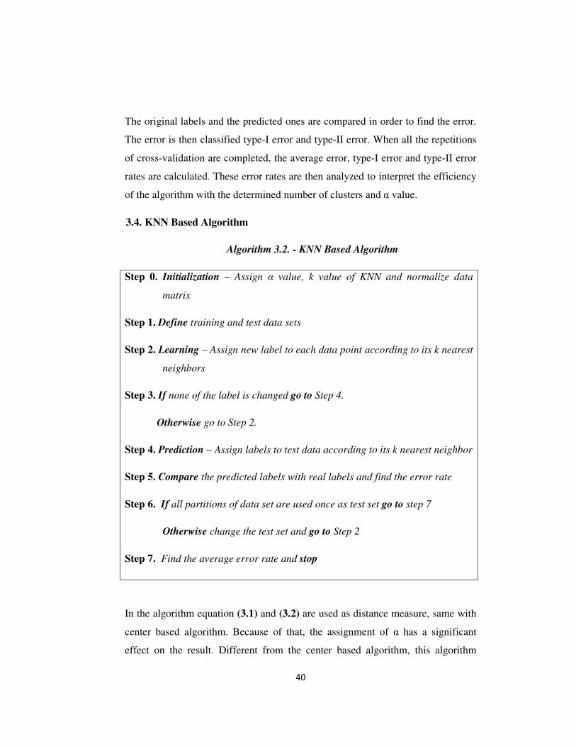
3.4. KNN Based Algorithm

Algorithm 3.2. - KNN Based Algorithm

Step 0. Initialization – Assign α value, k value of KNN and normalize data

matrix

Step 1. Define training and test data sets

Step 2. Learning – Assign new label to each data point according to its k nearest

neighbors

Step 3. If none of the label is changed go to Step 4.

Otherwise go to Step 2.

Step 4. Prediction – Assign labels to test data according to its k nearest neighbor

Step 5. Compare the predicted labels with real labels and find the error rate

Step 6. If all partitions of data set are used once as test set go to step 7

Otherwise change the test set and go to Step 2

Step 7. Find the average error rate and stop

In the algorithm equation (3.1) and (3.2) are used as distance measure, same with

center based algorithm. Because of that, the assignment of α has a significant

effect on the result. Different from the center based algorithm, this algorithm

41

requires the value of k for the number of neighborhood. By this assignment the

algorithm assigns the label to a data point according to the labels of its k nearest

neighbors. The structure of the data set may require normalizing operation in

initializing phase.

Splitting data set into training and test sets is a part of this methodology, too.

Similar with center based algorithm, the normalized data set split into ten parts.

Each of them used as test set once and remaining parts are used as training set. So

the steps 2, 3, 4 and 5 of the algorithm are repeated 10 times in the algorithm. This

means that ten-fold-cross-validation is used here which is previously explained in

section 2.5.1.

Each data point in data set has an original label. This methodology requires

assigning a new label to each data point, assigned label. k nearest neighbors of

each data point are taken into consideration and the dominated label is assigned to

the data point as assigned label. After completing the process for all the data

points in the data set, we control the number of data points that change its label. If

there is no data point that changes its label, algorithm continues with the next step.

Otherwise algorithm repeats the learning phase until the number of data points

that change its label drops to zero.

The prediction phase occurs similar with the learning phase, but executed once.

All data points in the learning phase gather an assigned label from the assigned

labels of its k nearest neighbors of training set. The difference between the

assigned labels and the original labels gives the error rate for current loop of

cross-validation process. After all loops are completed the average error rate can

be calculated to evaluate the performance of the algorithm.

42

CHAPTER 4

APPLICATION

Both algorithms are tested with generated data sets presented in Chapter 3. These

data sets are generated with MATLAB Version 7.5.0.342 (R2007b) by using the

source code shown in Appendix–B. All cases, named “separated”, “half-

separated”, “not-separated” are tested with different parameter values, using

center based heuristic and KNN based heuristic. Below, the figure shows the

classification success rate of center-based heuristic:

Center Based, Euclidean Distance, K = 2

Separable Case

Center Based, Euclidean Distance, K = 2

Half-Separable Case

Center Based, Euclidean Distance, K = 2

Not-Separable Case

Figure 4-1 Classification Success Rates of Center Based Heuristic with Euclidean

Distance

43

The u value is not effective on classification success rate in separable and half-

separable data sets. Appendix-C shows the success rates of both heuristics on the

data sets for different parameters.

After testing the algorithms by using generated data sets, both heuristics applied

to real biomedical data sets taken from University of California, Irvine. These data

sets contain the observations of different parameters in case of disease or health.

In addition to becoming real data sets, they have different number of dimensions

and also different numbers of classes (labels). The properties of these data sets are

shown in Table 4-1.

Table 4-1 Properties of biomedical data sets

Name Number of points Dimensions Labels

Breast Cancer 699 9 2

Diabetis 768 8 2

Hepatitis 155 19 2

Liver Cancer 345 6 2

Voting 435 16 2

Wine 178 13 3

In order to test the algorithms with these data sets, both algorithms executed with

different parameters. For center-based heuristic 2, 3 and 4 clusters are used with

an α scale. In this scale, α is increasing by 1 from 0 to 100. For KNN based

heuristic 3 nearest neighbors is used. In this algorithm 100 different α values are

also examined incrementing between 0 and 100. These experiments are performed

on a computer that is Pentium(R) Dual Core CPU with 2.20 GHz, 2GB installed

44

memory(RAM) and 32-bit operating system. The execution times are shown in

Table 4-2.

Table 4-2 Execution times with biomedical data sets

Data Set Time with Center-Based

Algorithm (seconds)

Time with KNN-Based

Algorithm (seconds)

Breast Cancer 11.22 132.99

Diabetis 14.20 259.57

Hepatitis 2.88 13.77

Liver Cancer 5.30 32.70

Voting 9.25 90.38

Wine 3.88 8.94

Appendix–C gives the classification success rates of heuristics on these data sets.

45

CHAPTER 5

DISCUSSIONS AND EVALUATIONS

In Chapter 4, two heuristics are applied on real data sets, there are lots of

experiments on generated data sets investigating the effects of parameters on

classification success rates. One of these parameters for center based heuristics is

the number of clusters, K. Although the success rates are changing according to

K, there is no pattern to conclude for number of clusters; but the only important

thing is choosing a cluster number greater than or equal to number of labels in the

data set. If not, there will be at least one label that is not assigned to any of the

clusters. It means that all data points which should have this particular label will

be assigned to another label and it cause incorrect predictions. One of the

biomedical data set “Wine” is a good example for this issue.

Wine Data Set, Mahalanobis Distance

K = 2

Wine Data Set, Mahalanobis Distance,

K = 3

Figure 5-1 Classification Success Rates of Wine Data Set (Center Based Heuristic

with Mahalanobis Distance)

46

Wine data set contains three labels. When two clusters are used in the algorithm,

the minimum error is around 34%, because all clusters are labeled with dominated

data points and at the end there are two labeled clusters. So, one or two labels are

used for labeling the clusters. It means that at least one label is not assigned to a

cluster. Any data point which has this label is assigned to one of the other labels,

causing high classification error rate. On the contrary, when 3 clusters are used in

the algorithm, all labels can be used for labeling the clusters. It provides an

opportunity to assign all data points to its real clusters. In this case error is

reduced to 7% (Figure 5-1).

Similarly choice of K in KNN based heuristic is also important. If K is an even

number, it can be difficult to find dominated label in a data point’s neighborhood.

When K is an even number, the points forced to be assigned arbitrarily in the case

of tie. For this reason the choice of odd number for K, is a better choice in KNN

based heuristics and K = 3 is used in this thesis. It is also possible to work with

bigger odd numbers instead of 3, but since all the neighbors have the same

importance in the heuristic, bigger K values lead to loose the local structure. This

would be against the logic of KNN based algorithm.

Since Mahalanobis distance takes the correlations within a data set between the

variable into consideration, this distance is used in both of the algorithms. The

main reason for this choice is the structure of biomedical data sets. Correlations

within the biomedical data sets make this distance type a better option for

heuristics. In addition to this, Euclidean distance is also used for testing the

heuristics in generated data sets.

The most important part of the algorithm, u value, has a strong effect up to a

level. The main effect of u is to help the clustering in training phase. It maps the

different labels to different areas in the new space, so classification becomes easy

comparing with the original space (Figure 3-6). Small u values means small

distances, large u values means large distances between these areas. This is why

the clustering error reduces while u is increasing. In some value of u, the distance

47

between these areas becomes so large which makes the clustering error zero. After

that value increasing u has no effect on clustering, since clustering error already

reaches zero. After that point the cluster centers and cluster labels can easily be

found without any error. This effect can also be seen on the result diagrams of the

algorithms. Error rates reduce up to a value and after that value, error rates get

settled down. (See Appendix-C)

It is also valid for KNN based heuristics. While u maps different labeled data

groups to different spaces, it increases the distances between different labeled data

points. This reduces the probability of including any data points to a

neighborhood of different labeled data point. When u reaches an optimal value,

this probability and also training error becomes zero.

The particular value of alpha that makes the training error zero varies according to

the structure of data set. If the data set contains separable classes, small alpha

values may be sufficient, since the training error is already very small without any

u value. On the contrary, half-separable or not-separable cases need higher

uvalues to decrease the classification error in the training set.

Dimensions of data set also affect the optimal value of u. The way that u supports

the training phase is adding a new dimension to data set. Adding a new dimension

to 2-dimensional data set is more effective than adding a new dimension to

20-dimensional space. Because in the second case there are many other

parameters that affect the distance calculation, so this additional dimension should

have more weight to make the same affect with first case, and this weight is u.

To sum up, u value decreases the error rate in the testing data but it may take

different values for different sets. Overall, higher the u value is, better the

classification success rate is. In six biomedical data sets, the error rates are

reduced by the help of u up to 8% comparing with the algorithms without u value

(or u = 0).

48

Table 5-1 Enhancement in Center Based Heuristic by u with biomedical data sets

Data Set α = 0 α = 100 ∆ Error

Breast Cancer 3,86% 3,83% 0,03%

Wine 7,02% 6,26% 0,76%

Voting 13,70% 11,46% 2,24%

Diabetis 34,50% 31,89% 2,61%

Hepatitis 48,88% 42,71% 6,17%

Liver Cancer 41,89% 33,77% 8,12%

Table 5-2 Enhancement in KNN Based Heuristic by u with biomedical data sets

Data Set α = 0 α = 100 ∆ Error

Breast Cancer 3,92% 3,53% 0,39%

Wine 5,77% 4,26% 1,51%

Voting 10,71% 9,77% 0,94%

Diabetis 26,48% 26,42% 0,06%

Hepatitis 42,49% 42,31% 0,18%

Liver Cancer 36,91% 34,73% 2,18%

49

CHAPTER 6

CONCLUSION AND FURTHER STUDIES

In this study, a new classification approach is examined. Information from class

labels is combined with information from variables (features) by mapping the

original space to a high dimensional space. In other words, a new kernel function

is created by using a distance measure combining the feature space and class

labels. This measure not only considers the distances between features but also the

distance between class labels with a predefined weight value, u. This approach is

implemented to two new heuristics which are tested with generated data sets and

real biomedical data sets.

In “center based heuristic”, u value does not affect the classification error rates

significantly in separable data sets. In contrary, u value affects the results on half-

separable and not-separable cases. Up to 8% of enhancement in classification

error rate is observed in biomedical data sets with center based heuristics. In

Breast Cancer data set even with zero value for u, high success classification rate

is obtained and incremented u value is not improving success rate. In Liver

Cancer data set with u = 0 classification success rate equals to 58% which is

improved up to 66% with high u values. Although Voting data set has high

classification success rate (86%) when u = 0, it also shows similar behavior with

high u values.

Changing distance basis from Euclidean distance to Mahalanobis distance also

increases the classification success rate, since the features are correlated in the

biomedical data sets. Mahalanobis Distance considering the correlations, works

better. On the contrary, for generated data sets, the effect of distance basis

becomes less important since there is no correlation. Unlike u value and distance

basis, number of clusters has no significant effect on classification success rates.

While the classification success rate improves with increasing K (number of

50

clusters) in Hepatitis data set, the classification success rate is affected negatively

with increasing K in Breast Cancer data set.

In KNN based heuristic, success rates are relatively high for low u values

comparing with center based algorithm. But the change with u value is not as high

as the previous algorithm. Similarly in the separable case, it is hard to say that

there is an effect of u on classification success rates. For not separable case, an

improvement in success rate is observed by increasing u value, but it is not as

effective as center based algorithm. The enhancement is up to 2% in biomedical

data sets. Because of the data structure, changing distance basis from Euclidean to

Mahalanobis also affects the results on biomedical data sets. Changing number of

neighbors, determined by the user in advance, in KNN based heuristic, has no

significant effect. But it is better to choose an odd number for the number of

neighbors.

In this study, a projection approach to a higher space (in training set) using a

compound distance measure combined feature space and class labels is developed.

The effect of label information, represented by u value, is investigated in

classification success rate. Although effect of label information measured with u

is different for center-based and KNN based heuristic, there is a common

behaviour in both algorithms. The improvement of the classification success rate

depends on the complexity of data set. In other words, u affects non-separable sets

more than separable sets. This common behaviour creates a question that should

be examined in further studies. Can u value be a measure for separability?

It is observed that only u value is not enough to define separability, but a function

of u with some other properties of data set, may produce meaningful results for

this issue. This study shows that the dimensions of data, or number of variables in

the data set, are important for effect ofu. In addition to this, algorithm used for

error calculation is also important for effect ofu. These observations give a clue

to find a separability measure for future research.

51

REFERENCES

Berry, M.J.A., Linoff, G.S., (2009), Data Mining Techniques: For Marketing,

Sales and Customer Relationship Management, 2nd

edition, New York:

Wiley Publishing

Besset, D.H., (2001), Object-Oriented Implementation of Numerical Methods: An

Introduction with Java and Smalltalk, California: Morgan Kaufmann

Bock, R.K., Krischer, W., (1998), The Data Analysis Briefbook, New York:

Springer-Verlag

Camps-Valls, G., Bruzzone, L., (2009), Kernel methods for Remote Sensing Data

Analysis, New Jersey: John Wiley and Sons

Cerrito, P.B., (2007), Introduction to Data Mining Using SAS Enterprise Miner,

North Carolina: SAS Publishing

Cios, K.J., Pedrycz, W., Swiniarski, R.W., Kurgan, L.A., (2007), Data Mining: A

Knowledge Discovery Approach, New York: Springer

Cumby, C., Roth, D., (2003), “On Kernel Methods for Relational Learning”,

Proceedings of the Twentieth International Conference on Machine

Learning (ICML-2003), Washington DC, Article accessed on 16th

April

2009, http://l2r.cs.uiuc.edu/~danr/Papers/CumbyRo03.pdf

Ertöz, L., Steinbach, M., Kumar, V., (2003), “Finding Clusters of Different Sizes,

Shapes, and Densities in Noisy, High Dimensional Data”, January 24 2003,

52

D. Barbara, C. Kamath, (Eds.), Proceedings of the Third SIAM International

Conference on Data Mining, Volume 3, 2003, San Francisco: SIAM

Eyob, E., (2009), Social Implications of Data Mining and Information Privacy:

Interdisciplinary Frameworks and Solutions, Pennsylvania: Idea Group Inc.

Gallus, D., Abecker, A., Richter, D., (2008), “Classification of Landslide

Susceptibility in the Development of Early Warning Systems”, A. Ruas, and

C. Gold, (Eds), 2008Headway in Spatial Data Handling, 13th

International

Symposium, Berlin Heidelberg: Springer-Verlag

Han, J., Kamber, M., (2006), Data Mining: Concepts and Techniques, 2nd

edition,

California: Morgan Kaufmann

Hand, D.J., Mannila, H., Smyth, P., (2001), Principles of Data Mining,

Massachusetts: MIT Press

Hearst, M.A., (1998), “Support Vector Machines”, IEEE Intelligent Systems and

Their Applications, July/August 1998, Vol. 13, Issue 4, pp. 18-28, ISSN

1094-

Hill, T., Lewicki, P., (2006), Statistics: Methods and Applications, A

Comprehensive Reference for Science, Tulsa: StatSoft Inc.

Iyigun, C., (2011), Clustering, The Wiley Encyclopedia of Operations Research

and Management Science (in print).

Kamen, E.W., Su, J.K., (1999), Introduction to optimal estimation, pp. 1, 1999,

Berlin Heidelberg: Springer-Verlag

Larose, D.T., (2005), Discovering Knowledge in Data: An Introduction to Data

Mining, New Jersey: John Wiley and Sons

Lee, D., Kim, M.H., (2002), “Data Mining”, Published in Leondes, C.T.,

Database and Data Communication Network Systems, Vol. 1, Copyright

2002, California: Elsevier Science (U.S.A.)

53

Leondes, C.T., (2005), Intelligent Knowledge-Based Systems: Volume 1:

Knowledge-based Systems, Norwell, Massachusetts; Birkhäuser & Kluwer

Academic Publishers

Li, A., Shi, Y., (2005), “An Integrated Classification Method: Combination of LP

and LDA”, X. Deng and Y. Ye, (Eds.): Internet and Network Economies:

First International Workshop, WINE 2005, LNCS 3828, pp. 758-767, 2005,

Berlin Heidelberg: Springer-Verlag

Maimon, O.Z., Rokach, L., (2005), Data Mining and Knowledge Discovery

Handbook, New York: Springer Science & Business

McLachlan, G.J., (1999), “Mahalanobis Distance”, RESONANCE, June 1999, pp.

20-26, Article accessed on 16th

April 2009,

http://www.ias.ac.in/resonance/June1999/pdf/June1999p20-26.pdf

Minh, L.H., An, L.T.H., Tao, P. D., (2006), “Hierarchical Clustering Based on

Mathematical Optimization”, W. K. Ng, M. Kitsuregawa, and J. Li, (Eds):

Advances in Knowledge Discovery and Data Mining: 10th

Pacific-Asia

Conference, PAKDD 2006, LNAI 3918, pp. 160-173, 2006, Berlin

Heidelberg: Springer-Verlag

Pedrycz, W., (2005), Knowledge-Based Clustering: From Data to Information

Granules, New Jersey: John Wiley & Sons

Priddy, K.L., Keller, P.E., (2005), Artificial Neural Networks, Washington: SPE

Press

Principe, J.C., Liu, W., Haykin S., (2010), Kernel Adaptive Filtering: A

Comprehensive Introduction, New Jersey: John Wiley and Sons

Rastegar, R., Rahmati, M., Meybodi, M.R., (2005), “A Clustering Algorithm

using Cellular Learning Automata Based Evolutionary Algorithm”, B.

Riberio, R.F. Albrecht, A. Dobnikar, (Eds), Adaptive and Natural

Computing Algorithm, New York: Springer-Verlag

54

Seber, G.A.F., (2004), Multivariate Observations, New Jersey: John Wiley and

Sons.

Shmueli. G., Patel, N.R., Bruce, P.C., (2008), Data Mining for Business

Intelligence: Concepts, Techniques, and Application in Microsoft Office

Excel with XLMiner, New York: John Wiley & Sons

Taylor, C.M., Agah, A., (2008), “Data Mining and Genetic Algorithms: Finding

Hidden Meaning in Biological and Biomedical Data”, T.G. Simolinski,

M.G. Milanova, A.E. Hassanien, (Eds.): Computational Intelligence in

Biomedical and Bioinformatics: Current Trends and Applications, SCI 151,

pp. 49-68, 2008, Berlin Heidelberg: Springer-Verlag

Thuraisingham, B., Awad, M., Khan, L., Wang, L., (2009), Design and

Implementation of Data Mining Tools, Florida: CRC Press.

Wrobel, S., Gärtner, T., Horváth, T., (2005), “Kernels for Predictive Graph

Mining”, From Data and Information Analysis to Knowledge Engineering,

Volume 2005-2006, New York: Springer-Verlag

Wübben, M., (2008), Analytical CRM: Developing and Maintaining Profitable

Customer Relationships in Non-Contractual Setting, 1st edition, Frankfurt:

Gabler Verlag

Zhang, Y., Su, H.Y., Jia, T., Chu, J., (2005), “Rule Extraction from Trained

Support Vector Machines”, T.B. Ho., D. Cheung, H. Liu, (Eds.): Advances

in Knowledge Discovery and Data Mining: 9th

Pacific-Asia Conference

PAKDD 2005, LNAI 3518, pp. 61-70, 2005, Berlin Heidelberg: Springer-

Verlag

55

APPENDICES

APPENDIX A

Algorithms in MATLAB

Center Based Algorithm

clear all

gennum = 500;

mu = [0 0];

SIGMA = [1 0; 0 0.2];

data1 = mvnrnd(mu,SIGMA,gennum);

unit = ones(gennum,1);

data1 = [data1 unit];

mu2 = [1 0];

data2 = mvnrnd(mu2,SIGMA,gennum);

unit = zeros(gennum,1);

data2 = [data2 unit];

data3 = [data1 ; data2] ;

[B,C] = size(data3); %% B==number of CMUPDATE = [];

%% Matrix for CMUPDATE2 = []; %% Matrix for

TRERROR = [];

TRAVER = [];

V = 10; %% Number of parts (Cross validation)

N = 10; %% Number of repeats (Cross validation)

%% 1) Variables

K = 3; %% K==number of clusters

for alfverr = 1 : 100

alf = alfverr / 10;

56

KONTROLX = alfverr

%% 2) Keep The Labels

data = data3 ;

for i = 1:B

LABEL(i,1) = i;

LABEL(i,2) = data(i,C);

data(i,C) = 0 ;

end

%% 3) Find STD Of Attributes

STD_MAT = std(data);

%% 4) Normalize Matrix

for i= 1:C

if STD_MAT(1,i)~= 0 %% To avoid dividing 0.

NORM_DATA(:,i) = data(:,i)/STD_MAT(i) ;

else

NORM_DATA(:,i) = 0 ;

end

end

%% 5) Repeat Cross Vaidation N Times

for h = 1 : N

%% 6)Divide The Set For Cross Validation

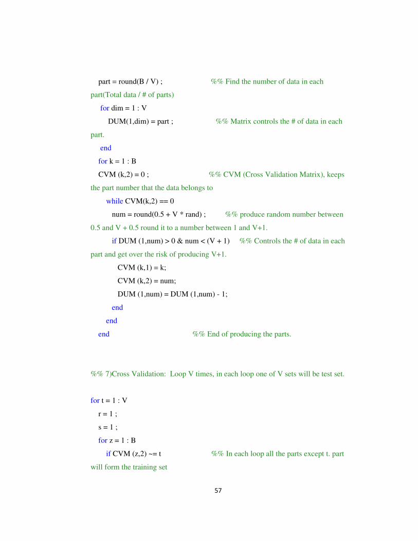
57

part = round(B / V) ; %% Find the number of data in each

part(Total data / # of parts)

for dim = 1 : V

DUM(1,dim) = part ; %% Matrix controls the # of data in each

part.

end

for k = 1 : B

CVM (k,2) = 0 ; %% CVM (Cross Validation Matrix), keeps

the part number that the data belongs to

while CVM(k,2) == 0

num = round(0.5 + V * rand) ; %% produce random number between

0.5 and V + 0.5 round it to a number between 1 and V+1.

if DUM (1,num) > 0 & num < (V + 1) %% Controls the # of data in each

part and get over the risk of producing V+1.

CVM (k,1) = k;

CVM (k,2) = num;

DUM (1,num) = DUM (1,num) - 1;

end

end

end %% End of producing the parts.

%% 7)Cross Validation: Loop V times, in each loop one of V sets will be test set.

for t = 1 : V

r = 1 ;

s = 1 ;

for z = 1 : B

if CVM (z,2) ~= t %% In each loop all the parts except t. part

will form the training set

58

TRAINING (r,:) = NORM_DATA (z,:) ; %% TRAINIG matrix

contains training data without labels.

TRAINING2 (r,:) = TRAINING (r,:) ;

TRAINING2 (r,C) = LABEL (z,2) ; %% TRAINIG2 matrix contains

training data with labels.

r = r + 1 ;

else %% t. part will be the test set

TEST (s,:) = NORM_DATA (z,:) ; %% TEST matrix contains test

data without labels.

TEST2 (s,:) = TEST (s,:) ;

TEST2 (s,C) = LABEL (z,2) ; %% TEST2 matrix contains test data

with labels.

s = s + 1 ;

end

end

r = r - 1; %% # of data in the training set

s = s - 1; %% # of data in the test set

%% 8)Initialine The Centers Of The Clusters

for u = 1 : K %% Initializing the centers or K clusters

CENTERS2(u,:) = TRAINING2 (u,:) ; %% CENTERS2 matrix

contains centers of clusters with labels.

CENTERS(u,:) = CENTERS2(u,:) ;

CENTERS(u,C) = 0 ; %% CENTERS matrix contains centers

of clusters without labels.

end

for v = 1 : r

CLUSTER(v,2) = 0 ; %% Initialize CLUSTER matrix.

end

59

%% 9)Produce The Distance Matrix (Initially Covariance Matrix = I)

CM = eye (C); %% Initialize Covariance Matrix as I.

for v = 1 : r %% Find the distances by using initial centers

and I as Covariance Matrix.

for w = 1 : K

DISTANCE (v,w) = sqrt(abs((TRAINING(v,:) -

CENTERS(w,:))*(TRAINING(v,:) - CENTERS(w,:))') + alf *

abs(TRAINING2(v,C) - CENTERS2(w,C)));

end

end

counter = 1 ;

%% 10)Determine The Centers Of Clusters

while counter ~= 0 %% Loop until the centers of clusters will

be determined.

counter = 0 ;

for v = 1 : r %% Assign data to the clusters.

[dis,cls] = min (DISTANCE (v,:)) ; %% Find the closest cluster.

CLUSTER (v,1) = v ;

if CLUSTER (v,2) ~= cls %% Control if the data transfers to

another cluster or not.

CLUSTER (v,2) = cls ; %% Assing new cluster number to the

data.

counter = counter + 1 ; %% Count the changes.

end

60

end %% End of assignments.

for w = 1 : K %% Update the centers.

for z = 1 : C

SUM(1,z) = 0 ;

end

NUMSUM = 0;

for v = 1 : r %% Find the new center by taking average of

the dimensions.

if CLUSTER (v,2) == w

SUM(1,:) = SUM(1,:) + TRAINING2(v,:) ;

NUMSUM = NUMSUM + 1;

CMUPDATE(NUMSUM,:) = TRAINING(v,:) ;

for m = 1 : (C-1)

CMUPDATE2(NUMSUM,m) = CMUPDATE(NUMSUM,m) ;

end

end

end

CENTERS2(w,:) = SUM(1,:) / NUMSUM ; %% Update the centers.

CENTERS2(w,C) = round (CENTERS2(w,C)) ; %% Find the labels of the

centers.

CENTERS (w,:) = CENTERS2 (w,:) ;

CENTERS (w,C) = 0 ; %% Unlabeled center matrix for

calculations.

for z = 1 : (C - 1)

TRAINING3(:,z) = TRAINING2(:,z) ; %% Unlabeled training matrix

for distance calculations.

CENTERS3(:,z) = CENTERS2(:,z) ; %% Unlabeled center matrix for

distance calculations.

61

TEST3(:,z) = TEST2(:,z) ; %% Unlabeled test matrix for distance

calculations.

end

COVMAT (:,:,w) = cov (CMUPDATE2) ; %% Update Covariance

Matrix for each cluster w.

end

for v = 1 : r %% Update DISTANCE matrix.

for w = 1 : K

DISTANCE (v,w) = sqrt(abs((TRAINING3(v,:) -

CENTERS3(w,:))*(TRAINING3(v,:) - CENTERS3(w,:))') + alf *

abs(TRAINING2(v,C) - CENTERS2(w,C)));

end

end

end %% Return line 106 until the centers of clusters

will be determined.

cntr = 0;

terr = 0;

TRERROR(alfverr,t) = 0;

for v = 2 : r

if CLUSTER(v,2) == CLUSTER ((v-1),2)

else

terr = terr + 1;

end

end

TRERROR(alfverr,t) = terr - K + 1;

%% 11)Test: Predict The Classes

62

for v = 1 : s

for w = 1 : K

CONTROL (v,w) = sqrt(abs((TEST3(v,:) - CENTERS3(w,:))*(TEST3(v,:) -

CENTERS3(w,:))'));

end

end

for v = 1 : s

[dis,cls] = min (CONTROL (v,:)) ; %% Find the minimum distance.

PREDIC (v,1) = v ;

PREDIC (v,2) = CENTERS2(cls,C) ; %% Predict the class according

to the label of cluster.

end

%% 12)Find The Errors For The Current Cross Validation

error = 0 ;

type1 = 0 ;

type2 = 0 ;

for v = 1 : s %% Compare the predictions with the real

data.

if PREDIC (v,2) ~= TEST2 (v,C)

error = error + 1; %% Add the error if there is a mismatch.

end

if PREDIC (v,2) > TEST2 (v,C)

type1 = type1 + 1; %% Add the error if there is an

overestimation.

end

if PREDIC (v,2) < TEST2 (v,C)

63

type2 = type2 + 1; %% Add the error if there is an

underestmation.

end

end

PERROR(h,t) = error / s ; %% Keep the errors for each run.

PTYPE1(h,t) = type1 / s ; %% Keep the errors for each run.

PTYPE2(h,t) = type2 / s ; %% Keep the errors for each run.

end

TRAVER(alfverr,2) = 0;

TRAVER(alfverr,1) = alfverr;

for v = 1 : V

TRAVER(alfverr,2) = TRAVER(alfverr,2)+ TRERROR(alfverr,V) ;

end

TRAVER(alfverr,2) = TRAVER(alfverr,2) / (V * r) ;

end

%% 13)Find The Average Errors

Avererror = (sum(PERROR(:)) / V) /N ; %% Find the averages of the

errors.

Avertype1 = (sum(PTYPE1(:)) / V) /N ; %% Find the averages of the

errors.

Avertype2 = (sum(PTYPE2(:)) / V) /N ; %% Find the averages of the

errors.

TOTERROR = [Avererror Avertype1 Avertype2]; %% Result Matrix

Log(alfverr,:) = [alf ([1 1 1] - TOTERROR)] ;

end

64

plot(Log(:,1)',Log(:,2)',':dg','MarkerFaceColor','g');

hold on ;

plot(Log(:,1)',Log(:,3)',':*b','MarkerFaceColor','b');

plot(Log(:,1)',Log(:,4)',':or','MarkerFaceColor','r');

hold off;

65

KNN Based Algorithm:

%% 0) Initialization

clear all;

gennum = 500;

mu = [0 0];

SIGMA = [1 0; 0 0.2];

data1 = mvnrnd(mu,SIGMA,gennum);

unit = ones(gennum,1);

data1 = [data1 unit];

mu2 = [8 0];

data2 = mvnrnd(mu2,SIGMA,gennum);

unit = zeros(gennum,1);

data2 = [data2 unit];

data3 = [data1 ; data2] ;

[B,C] = size(data3); %% B==number of data points &

C==dimension of data set

CMUPDATE = []; %% Matrix for Updating Covariance

Matrix (with labels)

CMUPDATE2 = []; %% Matrix for Updating Covariance

Matrix (without labels)

TRERROR = [];

TRAVER = [];

V = 10; %% Number of parts (Cross validation)

N = 10; %% Number of repeats (Cross validation)

%% 1) Variables

K = 3; %% K==number of clusters (KNN)

%% alf= coefficient in the distance

for alfverr = 1 : 100

alf = alfverr / 10;

%% alf = alfverr ;

66

KONTROLX = alfverr

%% 2) Keep The Labels

data = data3 ;

for i = 1:B

LABEL(i,1) = i;

LABEL(i,2) = data(i,C);

data(i,C) = 0 ;

end

%% 3) Find STD Of Attributes

STD_MAT = std(data);

%% 4) Normalize Matrix

for i= 1:C

if STD_MAT(1,i)~= 0 %% To avoid dividing 0.

NORM_DATA(:,i) = data(:,i)/STD_MAT(i) ;

else

NORM_DATA(:,i) = 0 ;

end

end

%% 5) Repeat Cross Vaidation N Times

for h = 1 : N

%% 6)Divide The Set For Cross Validation

part = round(B / V) ; %% Find the number of data in each

part(Total data / # of parts)

for dim = 1 : V

DUM(1,dim) = part ; %% Matrix controls the # of data in each

part.

end

for k = 1 : B

CVM (k,2) = 0 ; %% CVM (Cross Validation Matrix), keeps

the part number that the data belongs to

while CVM(k,2) == 0

67

num = round(0.5 + V * rand) ; %% produce random number between

0.5 and V + 0.5 round it to a number between 1 and V+1.

if DUM (1,num) > 0 & num < (V + 1) %% Controls the # of data in each

part and get over the risk of producing V+1.

CVM (k,1) = k;

CVM (k,2) = num;

DUM (1,num) = DUM (1,num) - 1;

end

end

end %% End of producing the parts.

%% 7)Cross Validation: Loop V times, in each loop one of V sets will be test set.

for t = 1 : V

r = 1 ;

s = 1 ;

for z = 1 : B

if CVM (z,2) ~= t %% In each loop all the parts except t. part

will form the training set

TRAINING (r,:) = NORM_DATA (z,:) ; %% TRAINIG matrix

contains training data without labels.

TRAINING2 (r,:) = TRAINING (r,:) ;

TRAINING2 (r,C) = LABEL (z,2) ; %% TRAINIG2 matrix contains

training data with labels.

r = r + 1 ;

else %% t. part will be the test set

TEST (s,:) = NORM_DATA (z,:) ; %% TEST matrix contains test

data without labels.

TEST2 (s,:) = TEST (s,:) ;

TEST2 (s,C) = LABEL (z,2) ; %% TEST2 matrix contains test data

with labels.

s = s + 1 ;

end

68

end

r = r - 1; %% # of data in the training set

s = s - 1; %% # of data in the test set

%% 8)Find the labels according to KNN

TRAINKNN2 (:,:) = TRAINING2 (:,:) ;

for b = 1 : r

for a = 1 : C

TRAINKNN (b,a) = TRAINKNN2 (b,a) ;

end

TRAINKNN (b,C+1) = TRAINKNN2 (b,C) ;

end

for b = 1 : r

for a = 1 : (C - 1)

TRAINXS (b,a) = TRAINKNN (b,a);

end

end

for i = 1 : r

for j = 1 : r

KNN(i,j) = 0 ;

end

end

m = 1 ;

while m ~= 0

i = 0 ;

j = 0 ;

m = 0 ;

COVKNN (:,:) = cov (TRAINXS) ;

for i = 1 : r

for j = 1 : r

KNN(i,j) = sqrt(abs((TRAINXS(i,:) - TRAINXS(j,:)) *(TRAINXS (i,:) -

TRAINXS (j,:))') + alf * abs(TRAINKNN(i,C+1) - TRAINKNN(j,C+1))) ;

69

end

end

i = 0 ;

j = 0 ;

u = 0 ;

w = 1 ;

for i = 1 : r

x = 0 ;

for u = 1 : K

v = 1000000 ;

for j = 1 : r

if i ~= j

if KNN (i,j) >= 0

if KNN (i,j) < v

v = KNN (i,j) ;

w = j;

end

end

end

end

if i ~= w

x = x + TRAINKNN (w,C+1) ;

end

KNN (i,w) = -1 ;

end

x = round (x / K) ;

if TRAINKNN (w,C+1) ~= x

m = m + 1 ;

TRAINKNN (w,C+1) = x ;

end

end

70

end

%% 11)Test: Predict The Classes

TESTKNN2 (:,:) = TEST2 (:,:) ;

for a = 1 : C

TESTKNN (:,a) = TESTKNN2 (:,a) ;

end

TESTKNN (:,C+1) = TESTKNN2 (:,C) ;

for b = 1 : s

for a = 1 : (C - 1)

TESTXS (b,a) = TESTKNN(b,a);

end

end

COVKNN (:,:) = cov ([TRAINXS;TESTXS]) ;

for i = 1 : s

for j = 1 : r

TKNN(i,j) = sqrt(abs((TESTXS(i,:) - TRAINXS (j,:))

*(TESTXS(i,:) - TRAINXS (j,:))'));

end

end

i = 0 ;

j = 0 ;

u = 0 ;

w = 1 ;

for i = 1 : s

x = 0 ;

for u = 1 : K

v = 1000000 ;

for j = 1 : r

if TKNN (i,j) >= 0

if TKNN (i,j) < v

v = TKNN (i,j) ;

71

w = j;

end

end

end

x = x + TRAINKNN (w,C+1) ;

TKNN (i,w) = -1 ;

end

x = round (x / K) ;

TESTKNN (i,C+1) = x ;

end

%% 12)Find The Errors For The Current Cross Validation

error = 0 ;

type1 = 0 ;

type2 = 0 ;

for v = 1 : s %% Compare the predictions with the real

data.

if TESTKNN (v,C) ~= TESTKNN (v,C+1)

error = error + 1; %% Add the error if there is a mismatch.

end

if TESTKNN (v,C) > TESTKNN (v,C+1)

type1 = type1 + 1; %% Add the error if there is an

overestimation.

end

if TESTKNN (v,C) < TESTKNN (v,C+1)

type2 = type2 + 1; %% Add the error if there is an

underestmation.

end

end

% Training error

terror = 0 ;

ttype1 = 0 ;

72

ttype2 = 0 ;

for v = 1 : r %% Compare the predictions with the real

data.

if TRAINKNN (v,C) ~= TRAINKNN (v,C+1)

terror = terror + 1; %% Add the error if there is a mismatch.

end

if TRAINKNN (v,C) > TRAINKNN (v,C+1)

ttype1 = ttype1 + 1; %% Add the error if there is an

overestimation.

end

if TRAINKNN (v,C) < TRAINKNN (v,C+1)

ttype2 = ttype2 + 1; %% Add the error if there is an

underestmation.

end

end

TPERROR(h,t) = terror / r ; %% Keep the errors for each run.

TPTYPE1(h,t) = ttype1 / r ; %% Keep the errors for each run.

TPTYPE2(h,t) = ttype2 / r ; %% Keep the errors for each run.

% End of training error

PERROR(h,t) = error / s ; %% Keep the errors for each run.

PTYPE1(h,t) = type1 / s ; %% Keep the errors for each run.

PTYPE2(h,t) = type2 / s ; %% Keep the errors for each run.

end

end

%% 13)Find The Average Errors

% training error

Trainerror = (sum(TPERROR(:)) / V) /N ; %% Find the averages of the

errors.

Traintype1 = (sum(TPTYPE1(:)) / V) /N ; %% Find the averages of the

errors.

73

Traintype2 = (sum(TPTYPE2(:)) / V) /N ; %% Find the averages of the

errors.

TTRERROR = [Trainerror Traintype1 Traintype2]; %% Result Matrix

TLog(alfverr,:) = [alf TTRERROR] ;

% training error

Avererror = (sum(PERROR(:)) / V) /N ; %% Find the averages of the

errors.

Avertype1 = (sum(PTYPE1(:)) / V) /N ; %% Find the averages of the

errors.

Avertype2 = (sum(PTYPE2(:)) / V) /N ; %% Find the averages of the

errors.

TOTERROR = [Avererror Avertype1 Avertype2]; %% Result Matrix

Log(alfverr,:) = [alf ([1 1 1] - TOTERROR)] ;

%%Log(alfverr,:) = [alf TOTERROR] ;

end

plot(Log(:,1)',Log(:,2)',':dg','MarkerFaceColor','g');

hold on ;

plot(Log(:,1)',Log(:,3)',':*b','MarkerFaceColor','b');

plot(Log(:,1)',Log(:,4)',':or','MarkerFaceColor','r');

hold off;

74

APPENDIX B

Source Code for Data Set Generation

a. Separated Data:

clear all

gennum = 500;

mu = [0 0];

SIGMA = [1 0; 0 0.2];

data1 = mvnrnd(mu,SIGMA,gennum);

unit = ones(gennum,1);

data1 = [data1 unit];

mu2 = [8 0];

data2 = mvnrnd(mu2,SIGMA,gennum);

unit = zeros(gennum,1);

data2 = [data2 unit];

data3 = [data1 ; data2] ;

b. Half-Separated Data:

clear all

gennum = 500;

mu = [0 0];

SIGMA = [1 0; 0 0.2];

data1 = mvnrnd(mu,SIGMA,gennum);

unit = ones(gennum,1);

data1 = [data1 unit];

mu2 = [4 0];

data2 = mvnrnd(mu2,SIGMA,gennum);

unit = zeros(gennum,1);

data2 = [data2 unit];

data3 = [data1 ; data2] ;

75

c. Not-Separated Data:

clear all

gennum = 500;

mu = [0 0];

SIGMA = [1 0; 0 0.2];

data1 = mvnrnd(mu,SIGMA,gennum);

unit = ones(gennum,1);

data1 = [data1 unit];

mu2 = [1 0];

data2 = mvnrnd(mu2,SIGMA,gennum);

unit = zeros(gennum,1);

data2 = [data2 unit];

data3 = [data1 ; data2] ;

76

APPENDIX C

Application in MATLAB

C.1. Center Based Algorithm

Center Based, Euclidean Distance, K = 3

Separable Case

Center Based, Euclidean Distance, K = 3

Half-Separable Case

Center Based, Euclidean Distance, K = 3

Not-Separable Case

Figure C-1 - Success Rate vs. u value, Center Based Algorithm with Euclidean

Distance

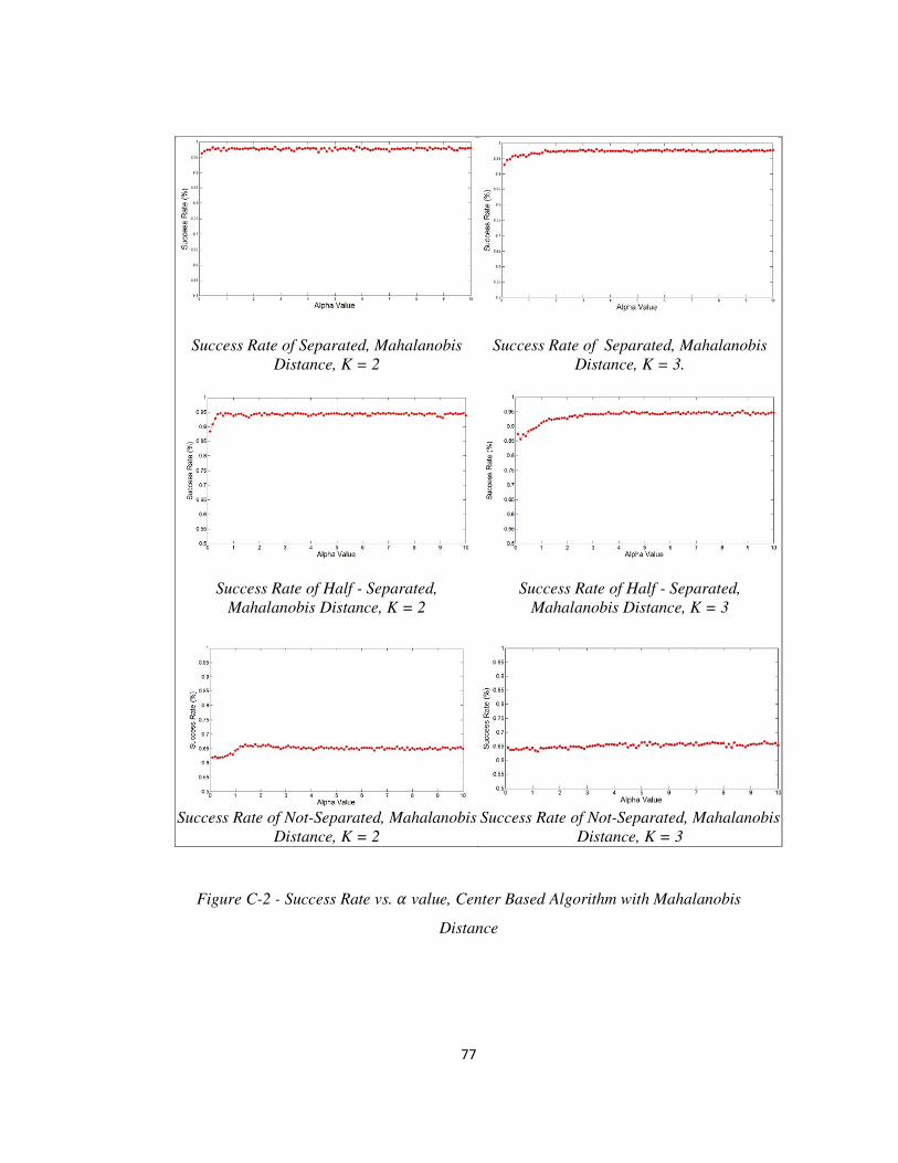
77

Success Rate of Separated, Mahalanobis

Distance, K = 2

Success Rate of Separated, Mahalanobis

Distance, K = 3.

Success Rate of Half - Separated,

Mahalanobis Distance, K = 2

Success Rate of Half - Separated,

Mahalanobis Distance, K = 3

Success Rate of Not-Separated, Mahalanobis

Distance, K = 2

Success Rate of Not-Separated, Mahalanobis

Distance, K = 3

Figure C-2 - Success Rate vs. u value, Center Based Algorithm with Mahalanobis

Distance

78

Success Rate of Separated, Euclidean

Distance, u = 10

Success Rate of Separated, Euclidean

Distance, u = 3

Success Rate of Separated, Euclidean

Distance, u = 1

Success Rate of Separated, Euclidean

Distance, u = 0.1

Figure C-3 - Success Rate vs. Number of Clusters, Center Based Algorithm on

Separated Data with Euclidean Distance

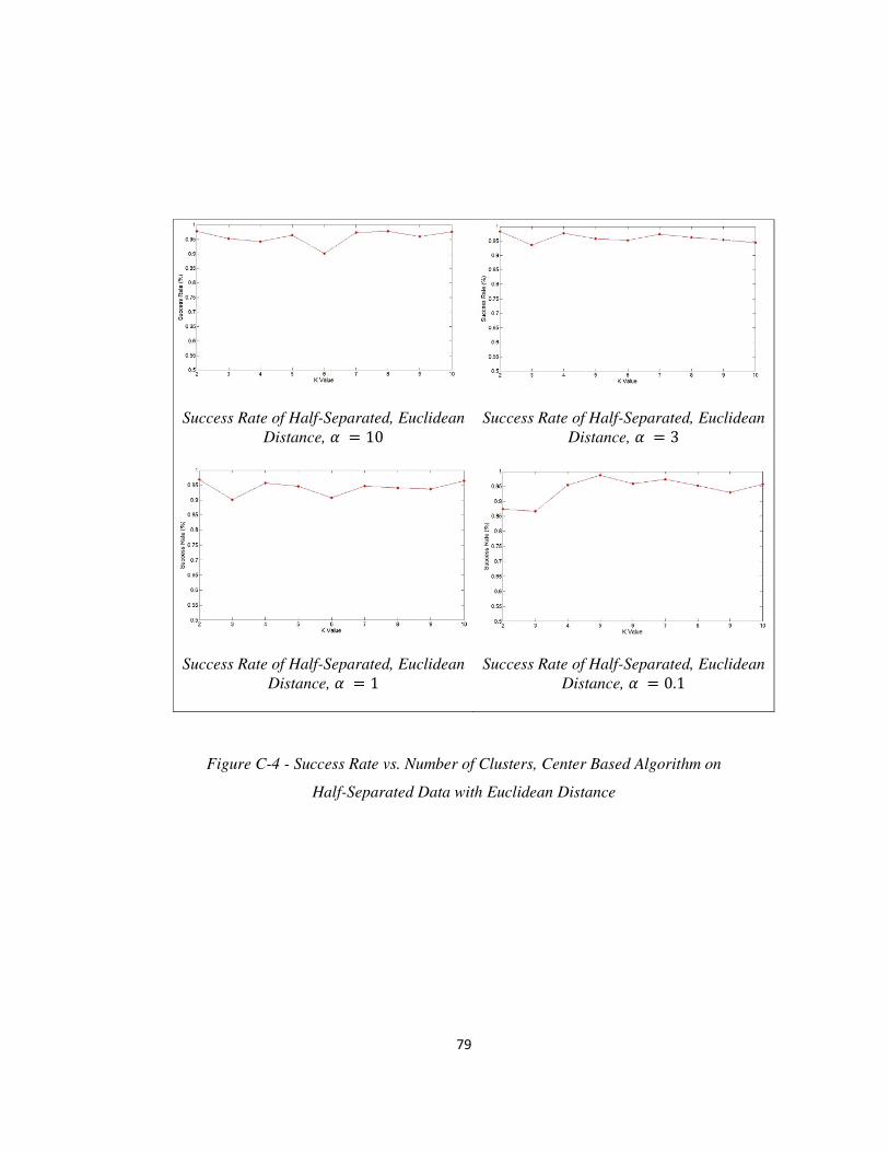
79

Success Rate of Half-Separated, Euclidean

Distance, u = 10

Success Rate of Half-Separated, Euclidean

Distance, u = 3

Success Rate of Half-Separated, Euclidean

Distance, u = 1

Success Rate of Half-Separated, Euclidean

Distance, u = 0.1

Figure C-4 - Success Rate vs. Number of Clusters, Center Based Algorithm on

Half-Separated Data with Euclidean Distance

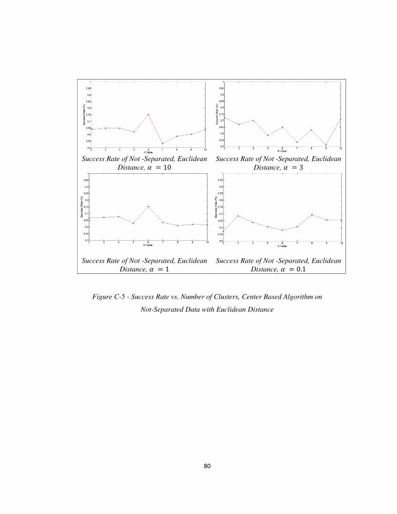
80

Success Rate of Not -Separated, Euclidean

Distance, u = 10

Success Rate of Not -Separated, Euclidean

Distance, u = 3

Success Rate of Not -Separated, Euclidean

Distance, u = 1

Success Rate of Not -Separated, Euclidean

Distance, u = 0.1

Figure C-5 - Success Rate vs. Number of Clusters, Center Based Algorithm on

Not-Separated Data with Euclidean Distance

81

Success Rate of Separated, Mahalanobis

Distance, u = 10

Success Rate of Separated, Mahalanobis

Distance, u = 3

Success Rate of Separated, Mahalanobis

Distance, u = 1

Success Rate of Separated, Mahalanobis

Distance, u = 0.1

Figure C-6 - Success Rate vs. Number of Clusters, Center Based Algorithm on

Separated Data with Mahalanobis Distance

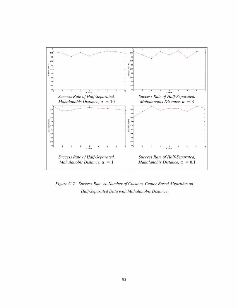
82

Success Rate of Half-Separated,

Mahalanobis Distance, u = 10

Success Rate of Half-Separated,

Mahalanobis Distance, u = 3

Success Rate of Half-Separated,

Mahalanobis Distance, u = 1

Success Rate of Half-Separated,

Mahalanobis Distance, u = 0.1

Figure C-7 - Success Rate vs. Number of Clusters, Center Based Algorithm on

Half-Separated Data with Mahalanobis Distance

83

Success Rate of Not-Separated, Mahalanobis

Distance, u = 10

Success Rate of Not-Separated,

Mahalanobis Distance, u = 3

Success Rate of Not-Separated, Mahalanobis

Distance, u = 1

Success Rate of Not-Separated, Mahalanobis

Distance, u = 0.1

Figure C-8 - Success Rate vs. Number of Clusters, Center Based Algorithm on

Not-Separated Data with Mahalanobis Distance

84

C.2. KNN Based Algorithm

Success Rate of Separated, Euclidean

Distance, K = 3

Success Rate of Separated, Mahalanobis

Distance, K = 3

Success Rate of Half-Separated, Euclidean

Distance, K = 3

Success Rate of Half-Separated,

Mahalanobis Distance, K = 3

Success Rate of Not-Separated, Euclidean

Distance, K = 3

Success Rate of Not-Separated,

Mahalanobis Distance, K = 3

Figure C-9 - Success Rate vs. u Value, KNN Based Algorithm

85

C.3. Center Based Algorithm Results on Biomedical Data sets

i. Diabetis:

Success rate of Diabetis, Mahalanobis

Distance, K = 2, uЄ[0100]

Success rate of Diabetis, Mahalanobis

Distance, K = 3, uЄ[0100]

Success rate of Diabetis, Mahalanobis

Distance, K = 4, uЄ[0100]

Success rate of Diabetis, Mahalanobis

Distance, u = 50

Figure C-10 - Success Rate of Diabetis Data Set, Center Based Algorithm with

Mahalanobis Distance

86

ii. Hepatitis:

Success rate of Hepatitis, Mahalanobis

Distance, K = 2, uЄ[0100]

Success rate of Hepatitis, Mahalanobis

Distance, K = 3, uЄ[0100]

Success rate of Hepatitis, Mahalanobis

Distance, K = 4, uЄ[0100]

Success rate of Hepatitis, Mahalanobis

Distance, u = 50

Figure C-11 - Success Rate of Hepatitis Data Set, Center Based Algorithm with

Mahalanobis Distance

87

iii. Liver Cancer:

Success Rate of Liver Cancer, Mahalanobis

Distance, K = 2, uЄ[0100]

Success Rate of Liver Cancer, Mahalanobis

Distance, K = 3, uЄ[0100]

Success Rate of Liver Cancer, Mahalanobis

Distance, K = 4, uЄ[0100]

Success Rate of Liver Cancer, Mahalanobis

Distance, u = 50

Figure C-12 - Success Rate of Liver Cancer Data Set, Center Based Algorithm

with Mahalanobis Distance

88

iv. Voting:

Success Rate of Voting, Mahalanobis

Distance, K = 2, uЄ[0100]

Success Rate of Voting, Mahalanobis

Distance, K = 3, uЄ[0100]

Success Rate of Voting, Mahalanobis

Distance, K = 4, uЄ[0100]

Success Rate of Voting, Mahalanobis

Distance, u = 50

Figure C-13 - Success Rate of Voting Data Set, Center Based Algorithm with

Mahalanobis Distance

89

v. Wine:

Success Rate of Wine, Mahalanobis

Distance, K = 2, uЄ[0100]

Success Rate of Wine, Mahalanobis

Distance, K = 3, uЄ[0100]

Success Rate of Wine, Mahalanobis

Distance, K = 4, uЄ[0100]

Success Rate of Wine, Mahalanobis

Distance, u = 50

Figure C-14 - Success Rate of Wine Data Set, Center Based Algorithm with

Mahalanobis Distance

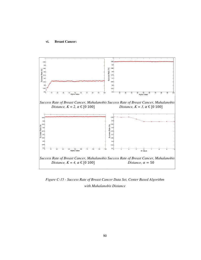
90

vi. Breast Cancer:

Success Rate of Breast Cancer, Mahalanobis

Distance, K = 2, uЄ[0100]

Success Rate of Breast Cancer, Mahalanobis

Distance, K = 3, uЄ[0100]

Success Rate of Breast Cancer, Mahalanobis

Distance, K = 4, uЄ[0100]

Success Rate of Breast Cancer, Mahalanobis

Distance, u = 50

Figure C-15 - Success Rate of Breast Cancer Data Set, Center Based Algorithm

with Mahalanobis Distance

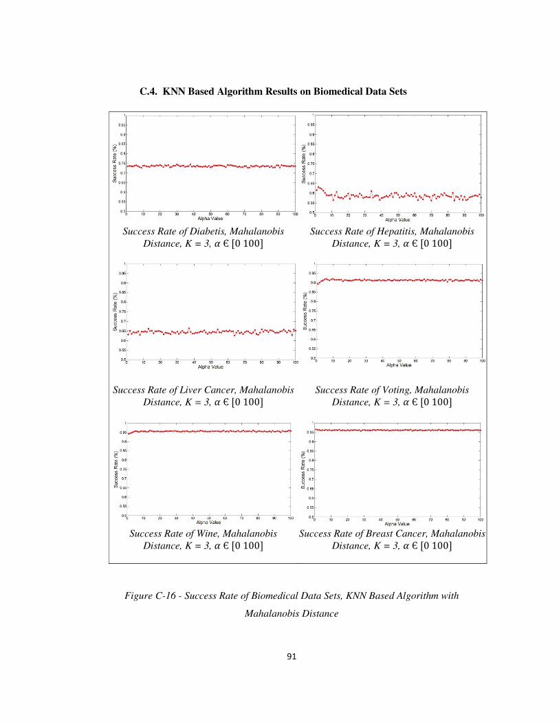
91

C.4. KNN Based Algorithm Results on Biomedical Data Sets

Success Rate of Diabetis, Mahalanobis

Distance, K = 3, uЄ[0100]

Success Rate of Hepatitis, Mahalanobis

Distance, K = 3, uЄ[0100]

Success Rate of Liver Cancer, Mahalanobis

Distance, K = 3, uЄ[0100]

Success Rate of Voting, Mahalanobis

Distance, K = 3, uЄ[0100]

Success Rate of Wine, Mahalanobis

Distance, K = 3, uЄ[0100]

Success Rate of Breast Cancer, Mahalanobis

Distance, K = 3, uЄ[0100]

Figure C-16 - Success Rate of Biomedical Data Sets, KNN Based Algorithm with

Mahalanobis Distance