A CLASSICALINTRODUCTIONTO GALOIS THEORY

A CLASSICALINTRODUCTIONTO GALOIS THEORY

STEPHEN C. NEWMANUniversity of Alberta,Edmonton, Alberta, Canada

A JOHN WILEY & SONS, INC., PUBLICATION

Copyright © 2012 by John Wiley & Sons, Inc. All rights reserved

Published by John Wiley & Sons, Inc., Hoboken, New JerseyPublished simultaneously in Canada

No part of this publication may be reproduced, stored in a retrieval system, or transmitted in anyform or by any means, electronic, mechanical, photocopying, recording, scanning, or otherwise,except as permitted under Section 107 or 108 of the 1976 United States Copyright Act, withouteither the prior written permission of the Publisher, or authorization through payment of theappropriate per-copy fee to the Copyright Clearance Center, Inc., 222 Rosewood Drive, Danvers,MA 01923, (978) 750-8400, fax (978) 750-4470, or on the web at www.copyright.com. Requeststo the Publisher for permission should be addressed to the Permissions Department, John Wiley &Sons, Inc., 111 River Street, Hoboken, NJ 07030, (201) 748-6011, fax (201) 748-6008, or online athttp://www.wiley.com/go/permission.

Limit of Liability/Disclaimer of Warranty: While the publisher and author have used their bestefforts in preparing this book, they make no representations or warranties with respect to theaccuracy or completeness of the contents of this book and specifically disclaim any impliedwarranties of merchantability or fitness for a particular purpose. No warranty may be created orextended by sales representatives or written sales materials. The advice and strategies containedherein may not be suitable for your situation. You should consult with a professional whereappropriate. Neither the publisher nor author shall be liable for any loss of profit or any othercommercial damages, including but not limited to special, incidental, consequential, or otherdamages.

For general information on our other products and services or for technical support, please contactour Customer Care Department within the United States at (800) 762-2974, outside the UnitedStates at (317) 572-3993 or fax (317) 572-4002.

Wiley also publishes its books in a variety of electronic formats. Some content that appears in printmay not be available in electronic formats. For more information about Wiley products, visit ourweb site at www.wiley.com.

Library of Congress Cataloging-in-Publication Data:

Newman, Stephen C., 1952–A classical introduction to Galois theory / Stephen C. Newman.

p. cm.Includes index.

ISBN 978-1-118-09139-5 (hardback)1. Galois theory. I. Title.QA214.N49 2012512′.32–dc23

2011053469

Printed in the United States of America

10 9 8 7 6 5 4 3 2 1

To Sandra

CONTENTS

PREFACE xi

1 CLASSICAL FORMULAS 1

1.1 Quadratic Polynomials / 31.2 Cubic Polynomials / 51.3 Quartic Polynomials / 11

2 POLYNOMIALS AND FIELD THEORY 15

2.1 Divisibility / 162.2 Algebraic Extensions / 242.3 Degree of Extensions / 252.4 Derivatives / 292.5 Primitive Element Theorem / 302.6 Isomorphism Extension Theorem and Splitting Fields / 35

3 FUNDAMENTAL THEOREM ON SYMMETRICPOLYNOMIALS AND DISCRIMINANTS 41

3.1 Fundamental Theorem on Symmetric Polynomials / 413.2 Fundamental Theorem on Symmetric Rational Functions / 483.3 Some Identities Based on Elementary Symmetric

Polynomials / 50

vii

viii CONTENTS

3.4 Discriminants / 533.5 Discriminants and Subfields of the Real Numbers / 60

4 IRREDUCIBILITY AND FACTORIZATION 65

4.1 Irreducibility Over the Rational Numbers / 654.2 Irreducibility and Splitting Fields / 694.3 Factorization and Adjunction / 72

5 ROOTS OF UNITY AND CYCLOTOMIC POLYNOMIALS 80

5.1 Roots of Unity / 805.2 Cyclotomic Polynomials / 82

6 RADICAL EXTENSIONS AND SOLVABILITY BYRADICALS 89

6.1 Basic Results on Radical Extensions / 896.2 Gauss’s Theorem on Cyclotomic Polynomials / 936.3 Abel’s Theorem on Radical Extensions / 1046.4 Polynomials of Prime Degree / 109

7 GENERAL POLYNOMIALS AND THE BEGINNINGS OFGALOIS THEORY 117

7.1 General Polynomials / 1177.2 The Beginnings of Galois Theory / 124

8 CLASSICAL GALOIS THEORY ACCORDING TO GALOIS 135

9 MODERN GALOIS THEORY 151

9.1 Galois Theory and Finite Extensions / 1529.2 Galois Theory and Splitting Fields / 156

10 CYCLIC EXTENSIONS AND CYCLOTOMIC FIELDS 171

10.1 Cyclic Extensions / 17110.2 Cyclotomic Fields / 179

11 GALOIS’S CRITERION FOR SOLVABILITYOF POLYNOMIALS BY RADICALS 185

12 POLYNOMIALS OF PRIME DEGREE 192

CONTENTS ix

13 PERIODS OF ROOTS OF UNITY 200

14 DENESTING RADICALS 225

15 CLASSICAL FORMULAS REVISITED 231

15.1 General Quadratic Polynomial / 23115.2 General Cubic Polynomial / 23315.3 General Quartic Polynomial / 236

APPENDIX A COSETS AND GROUP ACTIONS 245

APPENDIX B CYCLIC GROUPS 249

APPENDIX C SOLVABLE GROUPS 254

APPENDIX D PERMUTATION GROUPS 261

APPENDIX E FINITE FIELDS AND NUMBER THEORY 270

APPENDIX F FURTHER READING 274

REFERENCES 277

INDEX 281

PREFACE

The quadratic formula for solving polynomials of degree 2 has been known forcenturies, and it is still an important part of mathematics education. Less familiarare the corresponding formulas for solving polynomials of degrees 3 and 4. Theseexpressions are more complicated than their quadratic counterpart, but the factthat they exist comes as no surprise. It is therefore altogether unexpected thatno such formulas are available for solving polynomials of degrees 5 and higher.Why should this be so? A complete answer to this intriguing problem is providedby Galois theory. In fact, Galois theory was created precisely to address this andrelated questions about polynomials, a feature that might not be apparent froma survey of current textbooks on university level algebra. The reason for thischange in focus is that Galois theory long ago outgrew its origin as a methodof studying the algebraic properties of polynomials. The elegance of the modernapproach to Galois theory is undeniable, but the attendant abstraction tends toobscure the satisfying concreteness of the ideas that underlie and motivate thisprofoundly beautiful area of mathematics.

This book develops Galois theory from a historical perspective. Throughout,the emphasis is on issues related to the solvability of polynomials by radicals.This gives the book a sense of purpose, and far from narrowing the scope,it provides a platform on which to develop much of the core curriculum ofGalois theory. Classical results by Abel, Gauss, Kronecker, Lagrange, Ruffini,and, of course, Galois are presented as background and motivation leading up toa modern treatment of Galois theory. The celebrated criterion due to Galois forthe solvability of polynomials by radicals is presented in detail. The power ofGalois theory as both a theoretical and computational tool is illustrated by a studyof the solvability of polynomials of prime degree, by developing the theory of

xi

xii PREFACE

periods of roots of unity (due to Gauss), by determining conditions for a type ofdenesting of radicals, and by deriving the classical formulas for solving generalquadratic, cubic, and quartic polynomials by radicals.

The reader is expected to have a basic knowledge of linear algebra, but otherthan that the book is largely self-contained. In particular, most of what is neededfrom the elementary theory of polynomials and fields is presented in the earlychapters of the book, and much of the necessary group theory is provided in aseries of appendices. When planning and writing this book, I had in mind that itmight be used as a resource by mathematics students interested in understandingthe origins of Galois theory and the reason it was created in the first place. To thisend, proofs are quite detailed and there are numerous worked examples, whileon the other hand, exercises have not been included.

Several acknowledgements are in order. It is my pleasure to thank ProfessorDavid Cox of Amherst College, Professor Jean-Pierre Tignol of the Universitecatholique de Louvain, and Professor Al Weiss of the University of Alberta fortheir valuable comments on drafts of the manuscript. I am further indebted toProfessors Cox and Tignol for their exceptional books on Galois theory fromwhich I benefitted greatly (see the References section). The commutative dia-grams were prepared using the program diagrams.sty developed by Paul Taylor,who kindly answered technical questions on its use.

Needless to say, any errors or other shortcomings in the book are solelythe responsibility of the author. I am most interested in receiving yourcomments, which can be e-mailed to me at stephennewman@telus.net . Theinevitable corrections to follow will be posted and periodically updated on thewebsites http://www.stephennewman.net and ftp://ftp.wiley.com/public/sci_tech_med/galois_theory .

Finally, and most importantly, I want to thank my wife, Sandra, for her stead-fast support and encouragement throughout the writing of the manuscript. It isto her, with love, that this book is dedicated.

CHAPTER 1

CLASSICAL FORMULAS

The historical backdrop to this book is the search for methods of solvingpolynomial equations by radicals, a challenge embraced by many of the greatestmathematicians of the past. There are polynomial equations of any given degreen that can be solved in this way. For example, xn − 2 = 0 has such a solution,usually denoted by the symbol n

√2. The question that arises is whether there is

a solution by radicals of the so-called general equation of degree n ,

anxn + an−1xn−1 + · · · + a1x + a0 = 0

where the coefficients a0, a1, . . . , an are indeterminates. When a solution exists,it provides a “formula” into which numeric coefficients can be substituted forspecific cases. The quadratic formula for second degree equations is no doubtfamiliar to the reader (see the following discussion).

In fact, methods of solving quadratic equations were known to the Baby-lonians as long ago as 2000 B.C. The book Al Kitab Al Jabr Wa’al Muqabelah bythe Persian mathematician Mohammad ibn Musa al-Khwarizmi appeared around830 A.D. In this work, the title of which gives us the word “algebra,” techniquesavailable at that time for solving quadratic equations were systematized. Around1079, the Persian mathematician and poet Omar Khayyam (of Rubaiyat fame)presented a geometric method for solving certain cubic (third degree) equations.

An algebraic solution of a particular type of cubic equation was discoveredby the Italian mathematician Scipione del Ferro (1465–1526) around 1515, but

A Classical Introduction to Galois Theory, First Edition. Stephen C. Newman.© 2012 John Wiley & Sons, Inc. Published 2012 by John Wiley & Sons, Inc.

1

2 CLASSICAL FORMULAS

this accomplishment was not published in his lifetime. About 1535, a morecomplete set of solutions was developed by the Italian mathematician NiccoloFontana (ca 1500–1557), nicknamed “Tartaglia” (the “Stammerer”). Theseresults were further developed by another Italian mathematician, GirolamoCardano (1501–1576), who published them in his book Artis Magnae, Sive deRegulis Algebraicis (The Great Art, or the Rules of Algebra), which appearedin 1545. The solution of the quartic (fourth degree) equation was discoveredby yet another Italian mathematician, Ludovico Ferrari (1522–1565), a pupil ofCardano.

The next challenge faced by the mathematical scholars of the Renaissance wasto find the solution of the quintic (fifth degree) equation. Since the quadratic,cubic, and quartic equations had given up their secrets, there was every reasonto believe that with sufficient effort and ingenuity the same would be true ofthe quintic. Yet, despite the efforts of some of the greatest mathematicians ofEurope over the ensuing two centuries, the quintic equation remained stubbornlyresistant. In 1770, the Italian mathematician Joseph-Louis Lagrange (1736–1813,born Giussepe Lodovico Lagrangia) published his influential Reflexions sur laresolution algebrique des equations. In this journal article of over 200 pages,Lagrange methodically analyzed the known techniques of solving polynomialequations. The principles uncovered by Lagrange, along with his introduction ofwhat would ultimately become group theory, opened up an entirely new approachto the problem of solving polynomial equations by radicals.

Nevertheless, the methods developed by Lagrange did not lead to a solution ofthe general quintic. In 1801, the eminent German mathematician and scientist CarlFriedrich Gauss (1777–1855) published Disquisitiones Arithmeticae (NumberResearch), a landmark in which he demonstrated, among other things, that forany degree n , the roots of the polynomial equation xn − 1 = 0 can be expressedin terms of radicals. Despite this success, it seems that Gauss was of the opinionthat the general quintic equation could not be solved by radicals.

This was certainly the view held by the Italian mathematician and physicianPaolo Ruffini (1765–1822), who published a treatise of over 500 pages on thetopic in 1799. An important feature of his work was the extensive use of grouptheory, albeit in what would now be considered rudimentary form. Although spe-cific objections to the proofs Ruffini presented were not forthcoming, there seemsto have been a reluctance on the part of the mathematical community to accepthis claims. Perhaps this was related to the novelty of his approach, or maybe itwas simply because his proofs were excessively complex, and therefore suspect.Over the years, Ruffini greatly simplified his methods, but his arguments neverseemed to achieve widespread approval, at least not during his lifetime. A notableexception was the French mathematician Augustin-Louis Cauchy (1789–1857),who was supportive of Ruffini and an early contributor to the development ofgroup theory.

In any event, the matter was definitively settled by the Norwegian mathemati-cian Niels Henrik Abel (1802–1829) with the publication in 1824 of a succinctand accessible proof showing that it is impossible to solve the general quintic

QUADRATIC POLYNOMIALS 3

equation by radicals. This result, along with its various generalizations, will bereferred to here as the Impossibility Theorem . As remarkable as this achievementwas, the methods used by Abel shed relatively little light on why the quinticequation is insolvable.

This question was answered in a spectacular manner by the French mathe-matician Evariste Galois (1811–1832). In fact, his approach encompasses notonly general polynomial equations but also the more complicated case wherethe coefficients of the polynomial are numeric. In the manuscript Memoire surles conditions de resolubilite des equations par radicaux, submitted to the ParisAcademy of Sciences when he was just 18 years of age, and published posthu-mously 14 years after his tragic death, Galois provides the foundations for whatwould become the mathematical discipline with which his name has becomesynonymous.

This book presents an introduction to Galois theory along both classical andmodern lines, with a focus on questions related to the solvability of polynomialequations by radicals. The classical content includes theorems on polynomials,fields, and groups due to such luminaries as Gauss, Kronecker, Lagrange, Ruffini,and, of course, Galois. These results figured prominently in earlier expositions ofGalois theory but seem to have gone out of fashion. This is unfortunate because,aside from being of intrinsic mathematical interest, such material provides pow-erful motivation for the more modern treatment of Galois theory presented laterin this book.

Over the course of the book, three versions of the Impossibility Theoremare presented. The first relies entirely on polynomials and fields, the secondincorporates a limited amount of group theory, and the third takes full advantageof modern Galois theory. This progression through methods that involve moreand more group theory characterizes the first part of the book. The latter partof the book is devoted to topics that illustrate the power of Galois theory asa theoretical and computational tool, but again in the context of solvability ofpolynomial equations by radicals.

In this chapter, we derive the classical formulas for solving quadratic, cubic,and quartic polynomial equations by radicals. It is assumed that the polynomialshave coefficients in Q, the field of rational numbers. This choice of underlyingfield is made for the sake of concreteness, but the arguments to follow applyequally to “general” polynomials as defined in Chapter 7. The discussion pre-sented here is somewhat informal. In Chapter 2 and later in the book, we introduceconcepts that allow the material given below to be made more rigorous. Sugges-tions for further reading on the material in this chapter, and other portions of thebook devoted to classical topics, can be found in Appendix F.

1.1 QUADRATIC POLYNOMIALS

Let

f (x) = x 2 − ax + b (1.1)

4 CLASSICAL FORMULAS

be a quadratic polynomial with coefficients in Q. A root of f (x) is an elementα (in some field) such that f (α) = 0. It is a fundamental result that, since f (x)

has degree 2, there are precisely two such roots, which we denote by α1 and α2.Consequently, f (x) can be expressed as

f (x) = (x − α1)(x − α2). (1.2)

The roots of f (x) are given by the quadratic formula:

α1, α2 = a ± √a2 − 4b

2. (1.3)

Here and throughout, the notation ± is to be interpreted as follows: α1 corre-sponds to the + sign and α2 to the − sign. Accordingly, (1.3) is equivalentto

α1 = a + √a2 − 4b

2and α2 = a − √

a2 − 4b

2.

A corresponding interpretation is given to the notation ∓.To derive (1.3), we substitute x = y + a/2 into (1.1), producing the so-called

reduced quadratic polynomial

g(y) = y2 + p

where

p = −a2

4+ b.

The roots of g(y) are

β1, β2 = ±√−p = ±√a2 − 4b

2.

Setting βi = αi − a/2 for i = 1, 2, gives (1.3). It is readily verified that (1.2)holds:

f (x) =(

x − a + √a2 − 4b

2

)(x − a − √

a2 − 4b

2

). (1.4)

When α1 = α2, we say that f (x) has a repeated root . The preceding statementthat f (x) has two roots remains true, provided that we take the repetition of rootsinto account.

CUBIC POLYNOMIALS 5

The quantity a2 − 4b is referred to as the discriminant of f (x) and is denotedby disc(f ). We have from (1.3) that

disc(f ) = a2 − 4b = (α1 − α2)2. (1.5)

Thus, f (x) has a repeated root if and only if disc(f ) = 0. In this case, the repeatedroot is α1 = α2 = a/2, and (1.4) becomes

f (x) =(

x − a

2

)2. (1.6)

This gives us a way of deciding whether a quadratic polynomial has a repeatedroot based solely on its coefficients. We will see a significant generalization ofthis finding in Chapter 3.

The symbol√

a2 − 4b deserves a comment. In the absence of further con-ditions,

√a2 − 4b represents either of the two roots of x2 − (a2 − 4b). When

a2 − 4b > 0,√

a2 − 4b is a real number, and it is common practice to take√a2 − 4b to be the positive square root of a2 − 4b. To take a simpler example,√2 is typically regarded as the positive square root of 2, that is,

√2 = 1.414 . . .

The negative square root of 2 is then −√2 = −1.414 . . . The distinction between

the positive and negative square roots of 2 rests on metric properties of realnumbers. In this book, we are focused almost exclusively on algebraic matters.Accordingly, unless otherwise indicated,

√2 stands for either the positive or neg-

ative square root of 2. Expressed differently but more algebraically,√

2 representseither of the roots of x2 − 2. As such, we are not obligated to specify whether√

2 equals 1.414 . . . or −1.414 . . ., only that it is one of these two quantities;by default, −√

2 is the other. Returning to√

a2 − 4b, we observe that switchingfrom one root of x2 − (a2 − 4b) to the other merely interchanges the values ofα1 and α2, leaving us with the same two roots of f (x).

1.2 CUBIC POLYNOMIALS

Let

f (x) = x 3 − ax2 + bx − c (1.7)

be a cubic polynomial with coefficients in Q. Consistent with the quadratic case,f (x) has three roots, which we denote by α1, α2, and α3. To find formulas forthese roots, we resort to a series of ad hoc devices. First, we eliminate thequadratic term in (1.7) by making the substitution x = y + a/3. This producesthe reduced cubic polynomial

g(y) = y3 + py + q (1.8)

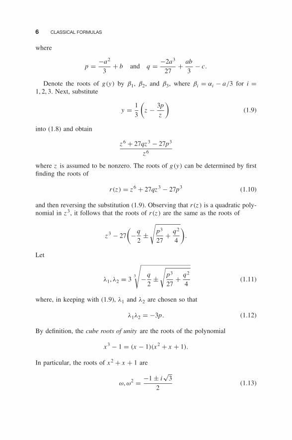
6 CLASSICAL FORMULAS

where

p = −a2

3+ b and q = −2a3

27+ ab

3− c.

Denote the roots of g(y) by β1, β2, and β3, where βi = αi − a/3 for i =1, 2, 3. Next, substitute

y = 1

3

(z − 3p

z

)(1.9)

into (1.8) and obtain

z 6 + 27qz 3 − 27p3

z 6

where z is assumed to be nonzero. The roots of g(y) can be determined by firstfinding the roots of

r(z ) = z 6 + 27qz 3 − 27p3 (1.10)

and then reversing the substitution (1.9). Observing that r(z ) is a quadratic poly-nomial in z 3, it follows that the roots of r(z ) are the same as the roots of

z 3 − 27

(−q

2±√

p3

27+ q2

4

).

Let

λ1, λ2 = 33

p−q

2±√

p3

27+ q2

4(1.11)

where, in keeping with (1.9), λ1 and λ2 are chosen so that

λ1λ2 = −3p. (1.12)

By definition, the cube roots of unity are the roots of the polynomial

x 3 − 1 = (x − 1)(x2 + x + 1).

In particular, the roots of x2 + x + 1 are

ω, ω2 = −1 ± i√

3

2(1.13)

CUBIC POLYNOMIALS 7

where, as usual, i = √−1. In (1.13), we take√

3 to be the positive square rootof 3. The notation ω will be reserved for (−1 + i

√3)/2 for the rest of the book.

We note in passing that

ω2 + ω + 1 = 0. (1.14)

It follows that the roots of r(z ) are

λ1 ωλ1 ω2λ1 λ2 ωλ2 and ω2λ2.

At first glance, it appears that the cubic polynomial g(y) also has six roots, whichis impossible. However, because of (1.12), the following identities hold:

1

3

(λ1 − 3p

λ1

)= λ1 + λ2

3= 1

3

(λ2 − 3p

λ2

)

1

3

(ω2λ1 − 3p

ω2λ1

)= ω2λ1 + ωλ2

3= 1

3

(ωλ2 − 3p

ωλ2

)

1

3

(ωλ1 − 3p

ωλ1

)= ωλ1 + ω2λ2

3= 1

3

(ω2λ2 − 3p

ω2λ2

).

The three roots of g(x) are therefore

β1 = λ1 + λ2

3

β2 = ω2λ1 + ωλ2

3

β3 = ωλ1 + ω2λ2

3.

(1.15)

Substituting from (1.11), we obtain

β1 = 3

p−q

2+√

p3

27+ q2

4+ 3

p−q

2−√

p3

27+ q2

4

β2 = ω2 3

p−q

2+√

p3

27+ q2

4+ ω

3

p−q

2−√

p3

27+ q2

4

β3 = ω3

p−q

2+√

p3

27+ q2

4+ ω2 3

p−q

2−√

p3

27+ q2

4

(1.16)

which are known as Cardan’s formulas .

8 CLASSICAL FORMULAS

Example 1.1. Setting p = 3 and q = 4, we have

g(y) = y3 + 3y + 4.

The graph of g(y) is shown below.

–2

–5

5

10

15

–10

0–1 1 2y

Clearly, g(y) has one real root, hence two nonreal complex roots. As suggestedby the graph, the real root is −1. We have from (1.16) that

β1 = 3√

−2 +√

5 + 3√

−2 −√

5

β2 = ω2 3√

−2 +√

5 + ω3√

−2 −√

5

β3 = ω3√

−2 +√

5 + ω2 3√

−2 −√

5.

(1.17)

The roots of x 2 − 5 are√

5 and −√5, and the three roots of x3 + 2 − √

5 are

3√

−2 +√

5 ω3√

−2 +√

5 and ω2 3√

−2 +√

5.

We now take√

5 and3√

−2 + √5 to be positive real numbers. For (1.12) to be

satisfied,3√

−2 − √5 = − 3

√2 + √

5 must be a negative real number. It can be

CUBIC POLYNOMIALS 9

shown that

3√

−2 +√

5 = −1 + √5

2and

3√

2 +√

5 = 1 + √5

2.

Using (1.13) and (1.14), we can simplify (1.17) to

β1 = −1 and β2, β3 = 1 ∓ i√

15

2. (1.18)

Alternatively, since −1 is a root of g(y), we have

g(y) = (y + 1)(y2 − y + 4)

which again leads to (1.18). ♦

Example 1.2. Setting p = −6 and q = −4, we have

g(y) = y3 − 6y − 4.

The graph of g(y) is shown below.

–4

–40

–30

–20

–10

10

20

30

0–3 –2 –1 1 2 3

y

4

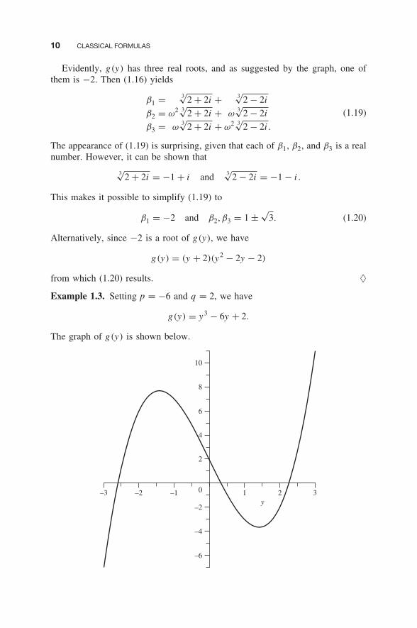
10 CLASSICAL FORMULAS

Evidently, g(y) has three real roots, and as suggested by the graph, one ofthem is −2. Then (1.16) yields

β1 = 3√

2 + 2i + 3√

2 − 2i

β2 = ω2 3√

2 + 2i + ω3√

2 − 2i

β3 = ω3√

2 + 2i + ω2 3√

2 − 2i .

(1.19)

The appearance of (1.19) is surprising, given that each of β1, β2, and β3 is a realnumber. However, it can be shown that

3√

2 + 2i = −1 + i and 3√

2 − 2i = −1 − i .

This makes it possible to simplify (1.19) to

β1 = −2 and β2, β3 = 1 ±√

3. (1.20)

Alternatively, since −2 is a root of g(y), we have

g(y) = (y + 2)(y2 − 2y − 2)

from which (1.20) results. ♦

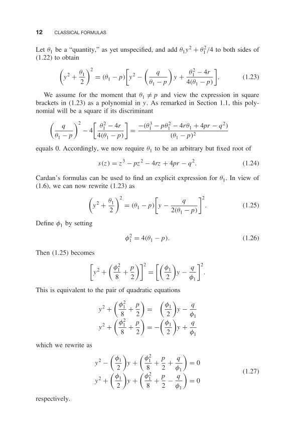
Example 1.3. Setting p = −6 and q = 2, we have

g(y) = y3 − 6y + 2.

The graph of g(y) is shown below.

–3 –2 –1

–6

–4

–2

2

4

6

8

10

0 1 2y

3

QUARTIC POLYNOMIALS 11

We see that g(y) has three real roots, but this time the numerical value of aroot is not empirically obvious. According to (1.16),

β1 = 3√

−1 + i√

7 + 3√

−1 − i√

7

β2 = ω2 3√

−1 + i√

7 + ω3√

−1 − i√

7

β3 = ω3√

−1 + i√

7 + ω2 3√

−1 − i√

7.

It is reasonable to expect that, just as in Example 1.2, we should be able toexpress β1, β2, and β3 entirely in terms of real numbers. Surprisingly, it is notpossible to do so, as will follow from Theorem 6.21. This counterintuitive resultis an example of a classical problem called the Casus Irreducibilis (IrreducibleCase). ♦

1.3 QUARTIC POLYNOMIALS

Let

f (x) = x 4 − ax3 + bx2 − cx + d (1.21)

be a quartic polynomial with coefficients in Q, and denote its roots by α1, α2,α3, and α4. Analogous to the approach used to solve the quadratic and cubicpolynomials, we begin by substituting x = y + a/4 into (1.21) and obtain thereduced quartic polynomial

g(y) = y4 + py2 + qy + r

where

p = −3a2

8+ b q = −a3

8+ ab

2− c

and

r = −3a4

256+ a2b

16− ac

4+ d .

Denote the roots of g(y) by β1, β2, β3, and β4, where βi = αi − a/4 for i =1, 2, 3, 4. To find the roots of g(y), we again resort to a series of contrivances.First, rewrite g(y) = 0 as

y4 = −py2 − qy − r . (1.22)

12 CLASSICAL FORMULAS

Let θ1 be a “quantity,” as yet unspecified, and add θ1y2 + θ21 /4 to both sides of

(1.22) to obtain(y2 + θ1

2

)2

= (θ1 − p)

[y2 −

(q

θ1 − p

)y + θ2

1 − 4r

4(θ1 − p)

]. (1.23)

We assume for the moment that θ1 �= p and view the expression in squarebrackets in (1.23) as a polynomial in y . As remarked in Section 1.1, this poly-nomial will be a square if its discriminant(

q

θ1 − p

)2

− 4

[θ2

1 − 4r

4(θ1 − p)

]= −(θ3

1 − pθ21 − 4rθ1 + 4pr − q2)

(θ1 − p)2

equals 0. Accordingly, we now require θ1 to be an arbitrary but fixed root of

s(z ) = z 3 − pz 2 − 4rz + 4pr − q2. (1.24)

Cardan’s formulas can be used to find an explicit expression for θ1. In view of(1.6), we can now rewrite (1.23) as(

y2 + θ1

2

)2

= (θ1 − p)

[y − q

2(θ1 − p)

]2

. (1.25)

Define φ1 by setting

φ21 = 4(θ1 − p). (1.26)

Then (1.25) becomes[y2 +

(φ2

1

8+ p

2

)]2

=[(

φ1

2

)y − q

φ1

]2

.

This is equivalent to the pair of quadratic equations

y2 +(

φ21

8+ p

2

)=

(φ1

2

)y − q

φ1

y2 +(

φ21

8+ p

2

)= −

(φ1

2

)y + q

φ1

which we rewrite as

y2 −(

φ1

2

)y +

(φ2

1

8+ p

2+ q

φ1

)= 0

y2 +(

φ1

2

)y +

(φ2

1

8+ p

2− q

φ1

)= 0

(1.27)

respectively.

QUARTIC POLYNOMIALS 13

Denote the roots of the first equation in (1.27) by β1 and β2, and those of thesecond by β3 and β4. We then have

β1, β2 = φ1

4± 1

2

√−φ2

1

4− 2p − 4q

φ1

β3, β4 = −φ1

4± 1

2

√−φ2

1

4− 2p + 4q

φ1

(1.28)

which will be referred to as Ferrari’s formulas . Note that if we replace φ1 with−φ1 in (1.28), we obtain the same roots for g(y) but with the rows of (1.28)reversed.

It remains to consider the case θ1 = p. In this situation, (1.24) becomes

s(z ) = z 3 − θ1z 2 − 4rz + 4θ1r − q2.

Then s(θ1) = 0 implies that q = 0, hence g(y) = y4 + py2 + r . This is aquadratic polynomial in y2, the roots of which are easily found.

Example 1.4 (5th root of unity). Consider the polynomial

�5(x) = x 4 + x3 + x2 + x + 1.

The reason for the choice of notation will be made clear in Chapter 5. Wereturn to �5(x) several times later in the book. To give �5(x) a more familiarinterpretation, observe that

x5 − 1 = (x − 1)�5(x).

In the terminology of Chapter 5, the roots of x5 − 1 are the 5th roots of unity.More specifically, the roots of �5(x) are ζ5, ζ 2

5 , ζ 35 , and ζ 4

5 , where

ζ5 = cos

(2π

5

)+ i sin

(2π

5

).

The reduced polynomial corresponding to �5(x) is

g(y) = y4 +(

5

8

)y2 +

(5

8

)y + 205

256.

In the above notation,

s(z ) = z 3 −(

5

8

)z 2 −

(205

64

)z + 825

512.

14 CLASSICAL FORMULAS

The reduced polynomial corresponding to s(z ) is

h(y) = y3 −(

10

3

)y + 25

27.

Using Cardan’s formulas, we find that h(y) has the roots

5

3and − 5

6±

√5

2.

It follows that the roots of s(z ) are

15

8and − 5

8±

√5

2.

The respective values of φ1 are

√5 and

√−5 ± 2

√5.

Choosing φ1 = √5 and taking all square roots to be positive, we find from

Ferrari’s formulas that the roots of �5(x) are

ζ5, ζ 45 = −1 + √

5 ± i√

10 + 2√

5

4

ζ 25 , ζ 3

5 = −1 − √5 ± i

√10 − 2

√5

4.

(1.29)

In (1.29), the assignment of the powers of ζ5 to their expressions in terms ofradicals was made on the basis of their respective numerical values. ♦

CHAPTER 2

POLYNOMIALS AND FIELD THEORY

This chapter provides the background material on polynomials and fields neededas a foundation for the remainder of the book. We begin with a few remarks onnotation. The ring of integers will be denoted by Z, and the fields of rational,real, and complex numbers by Q, R, and C, respectively. The letters E , F , K ,and L will always denote fields; x , y , and z will always denote indeterminates;and m and n will always denote integers, usually natural numbers.

Recall that a field F has characteristic 0 if for all natural numbers n ,

1 + 1 + · · · + 1 �= 0. [n terms]

Otherwise F is said to have nonzero characteristic. Any field of characteristic 0contains an isomorphic copy of Q. If F has nonzero characteristic, then thesmallest natural number n violating the characteristic 0 property is a prime, sayp. In this case, F is said to have characteristic p. Up to isomorphism, there is aunique field Fp of p elements, and it has characteristic p. We adopt the followingconvention:

With the exception of F in Theorem E.3, all fields other than Fp are assumedto have characteristic 0.

Most of the results to follow do not require such a strong assumption, but weproceed on this basis as a matter of convenience, and because it is the classicalcase.

A Classical Introduction to Galois Theory, First Edition. Stephen C. Newman.© 2012 John Wiley & Sons, Inc. Published 2012 by John Wiley & Sons, Inc.

15

16 POLYNOMIALS AND FIELD THEORY

2.1 DIVISIBILITY

We denote by F [x ] the ring of polynomials in x with coefficients in the field F .An element f (x) of F [x ] is said to be a polynomial over F . Let

f (x) = anxn + an−1xn−1 + · · · + a1x + a0.

For convenience of notation, we sometimes denote f (x) by f . By writing f (x)

in this manner, it is implicit, here and throughout, that an �= 0, except whenn = 0 and a0 = 0. We refer to an as the leading coefficient of f (x). If an = 1,f (x) is said to be a monic polynomial . When n = 0, in which case f (x) = a0,we say that f (x) is a constant polynomial . If f (x) is a constant polynomial anda0 = 0, that is, f (x) = 0, we refer to f (x) as the zero polynomial . (It will be clearfrom the context when the expression f (x) = 0 is meant to indicate that f (x) isthe zero polynomial, and when it represents a nonzero polynomial equation tobe “solved” for x .)

If f (x) is a nonzero polynomial, its degree is defined to be deg(f ) = n . Inparticular, the degree of a nonzero constant polynomial is 0. The degree of thezero polynomial is not defined . Let g(x) be a nonzero polynomial in F [x ]. We saythat g(x) divides f (x), or that g(x) is a divisor of f (x), if there is a polynomialh(x) in F [x ] such that f (x) = g(x)h(x).

Theorem 2.1 (Division Algorithm). Let f (x) and g(x) be nonzero polynomialsin F [x ]. Then there are unique polynomials q(x) and r(x) in F [x ] such that

f (x) = q(x)g(x) + r(x)

with deg(r) < deg(g) or r(x) = 0. If f (x) and g(x) are in Z[x ] and g(x) ismonic, then q(x) and r(x) are also in Z[x ].

Proof. Let

f (x) = anxn + an−1xn−1 + · · · + a1x + a0

and

g(x) = bmxm + bm−1xm−1 + · · · + b1x + b0.

Recall the convention that an , bm �= 0. If m > n , we set q(x) = 0 and r(x) = f (x).For m ≤ n , the proof is by induction on n . Suppose that n = 0. Then m = 0,hence f (x) = a0 �= 0 and g(x) = b0 �= 0. In this case, we set q(x) = a0/b0 andr(x) = 0. Now, assume that n ≥ 1 and let

h(x) = f (x) −(

an

bm

)xn−mg(x).