A class of neutral to the right priors inducedby superposition of beta processes

Pierpaolo De BlasiStefano FavaroPietro Muliere

No. 130

December 2009

www.carloalberto.org/working_papers

© 2009 by Pierpaolo De Blasi, Stefano Favaro and Pietro Muliere. Any opinions expressed here arethose of the authors and not those of the Collegio Carlo Alberto.

A class of neutral to the right priors induced by superpositionof beta processes

P. De Blasi1, S. Favaro2, P. Muliere3

1 Universita degli Studi di Torino and Collegio Carlo Alberto, Torino, Italy.

E-mail : pierpaolo.deblasi@unito.it

2 Universita degli Studi di Torino and Collegio Carlo Alberto, Torino, Italy.

E-mail : stefano.favaro@unito.it

3 Universita L. Bocconi, Milano, Italy.

E-mail : pietro.muliere@unibocconi.it

October 2009

Abstract

A random distribution function on the positive real line which belongs to the class of

neutral to the right priors is defined. It corresponds to the superposition of independent

beta processes at the cumulative hazard level. The definition is constructive and starts

with a discrete time process with random probability masses obtained from suitably defined

products of independent beta random variables. The continuous time version is derived as

the corresponding infinitesimal weak limit and is described in terms of completely random

measures. It takes the interpretation of the survival distribution resulting from independent

competing failure times. We discuss prior specification and illustrate posterior inference on

a real data example.

Key words and phrases: Bayesian nonparametrics, beta process, beta-Stacy process, com-

pletely random measures, neutral to the right priors, survival analysis

1 Introduction

Let FR+ be the space of all cumulative distribution functions on the positive real line. In this

paper we introduce a stochastic process Ft, t ≥ 0 with trajectories in FR+ which belongs to

the class of neutral to the right (NTR) priors. A random distribution function F on R+ is NTR

if, for any 0 ≤ t1 < t2 < . . . < tk <∞ and for any k ≥ 1, the random variables (r.v.s)

Ft1 ,Ft2 − Ft11− Ft1

, . . . ,Ftk − Ftk−1

1− Ftk−1

(1)

are independent, see Doksum (1974). NTR priors share some remarkable theoretical properties,

among which the most celebrated one is the conjugacy with respect to right-censored survival

1

data. The form of the posterior distribution and its large sample properties are now well known

(see, e.g., Ferguson and Phadia (1979), Kim and Lee (2001, 2004). An interesting extension

of NTR priors has been recently introduced by James (2006) with the family of spatial NTR

processes.

NTR priors can be represented as suitable transformations of completely random measures

(CRMs), i.e. random measures that give rise to mutually independent random variables when

evaluated on pairwise disjoint sets. Appendix A.1 provides a brief account of CRMs, as well

as justification of the following statements. It is important to recall that F is NTR if and

only if Ft = 1 − e−µ((0,t]) for some CRM µ on B(R+) (Borel σ-algebra of R+) such that

P[limt→∞ µ((0, t]) = ∞] = 1. The nonatomic part of µ (that is the part without fixed jumps)

is characterized by its Levy intensity ν, which is a nonatomic measure on R+ × R+, so that

the law of F is uniquely determined by ν and the density of the fixed jumps. The conjugacy

property of NTR priors can be then expressed as follows: the posterior distribution of F , given

(possibly) right-censored data, is described by a NTR process for a CRM µ∗ with fixed jump

points at uncensored observations. This result is of great importance for statistical inference;

indeed, the posterior distribution, conditional on right-censored data, is still NTR and one can

fully describe the associated CRM in terms of the updated Levy intensity and the densities of

the jumps at fixed points of discontinuity. Therefore, one can resort to the simulation algorithm

suggested in Ferguson and Klass (1972) to sample the trajectories of the underlying CRM, thus

obtaining approximate evaluations of posterior inferences.

The beta-Stacy process of Walker and Muliere (1997) is an important example of NTR prior.

Its main properties are (i) a parametrization with a straightforward interpretation in terms of

survival analysis that facilitates prior specification; (ii) a simple description of the posterior

process in terms of the parametrization used in the prior. For later reference, we recall these

two properties. As for (i), we adopt the parametrization in Walker and Muliere (1997, Definition

3) and we suppose, as is usual in applications, that the underlying CRM µ does not have fixed

jump points in the prior. To this end, let α be a diffuse measure on B(R+) and β : R+ → R+

a piecewise continuous and positive function such that∫ t

0 β(x)−1α(dx) → +∞ as t → +∞. A

beta-Stacy process Ft, t > 0 with parameter (α, β) is NTR for a CRM µ whose Levy intensity

is defined by

ν(ds, dx) =ds

1− e−se−sβ(x) α(dx). (2)

In particular, E(Ft) = 1−exp−∫ t

0 β(x)−1α(dx), see equation (32) in Appendix A.1, suggesting

that H0(t) =∫ t

0 β(x)−1α(dx) takes on the interpretation of the prior guess at the cumulative

hazard rate of F . The role played by α and β is better explained when one considers the

nonparametric distribution induced by the beta-Stacy process on the space of cumulative hazard

2

functions, i.e. the stochastic process Ht, t > 0 defined as

Ht = Ht(F ) =

∫ t

0

dFx1− Fx−

. (3)

It can be shown that Ht, t > 0 is distributed as a beta process of Hjort (1990) (see the

forthcoming Remark 3.1), so that E(Ht) = H0(t) and Var(Ht) =∫ t

0 [β(x)+1]−1dH0(x). Then, β

plays the role of concentration parameter: a large β makes for tighter concentration around H0.

As for (ii), consider data (T1,∆1) . . . , (Tn,∆n) arising from n lifetimes subject to right censoring,

where T stands for the time observed and ∆ is the censoring indicator (∆ = 1 indicates an exact

observation, ∆ = 0 a censored one). We adopt a point process formulation, which is standard

in survival analysis, by defining N(t) =∑

i≤n 1(Ti≤t,∆i=1) and Y (t) =∑

i≤n 1(Ti≥t). Based

on this notation, one can describe the posterior distribution of F as a beta-Stacy process,

that is Ft|data = 1 − e−µ∗((0,t]) where µ∗ is a CRM with fixed jumps defined by (2) with

updated parameter (α, β + Y ) and fixed jumps Vk, k ≥ 1 at locations tk, k ≥ 1 such that

1 − e−Vk ∼ beta(Ntk, β(tk) + Y (tk) −Ntk). Here, beta(a, b) denotes the beta distribution

and Ntk = N(tk)−N(t−k ) is the number of uncensored observations occurring at time tk.

Our aim is to introduce a new class of NTR priors and to investigate its properties with

respect to (i) and (ii). The definition is constructive and starts with a discrete time process

which satisfies the independence condition in (1). Following the idea of Walker and Muliere

(1997), we adopt a stick breaking construction: let 0 < t1 < t2 < . . . be a countable sequence of

time points indexed by k = 1, 2, . . . and define

Ftk =

k∑j=1

Vj

j−1∏l=1

(1− Vl) (4)

for V1, V2, . . . a sequence of independent r.v.s with values in the unit interval. Each Vj is recov-

ered from the product of independent beta distributed r.v.s so that the conditional probability

of an event at time tk given survival at time tk−1 is the result of a series of m independent

Bernoulli experiments. In Section 2, we discuss properties and possible simplifications of the

proposed parametrization, then we provide formulas for the finite dimensional distributions.

The continuous time version of the process is derived through a passage to the limit which leads

to the specification of the underlying CRM in terms of a Levy intensity of the form (see the

forthcoming Theorem 2.1)

ν(ds, dx) =ds

1− e−s

m∑i=1

e−sβi(x)αi(dx).

The beta-Stacy process can be recovered as a particular case either by setting m = 1 or by taking

βi = β for any i. In Section 3, we provide discussion on the proposed NTR prior by studying

3

the induced distribution on the space of cumulative hazard functions. One obtains that the

corresponding random cumulative hazard is given by the superposition of m independent beta

processes (see the forthcoming Proposition 3.1), which motivates the name m-fold beta NTR

process we will give to the new prior. It also suggests that the prior beliefs can be specified

reasoning in terms of survival times generated by independent competing failure times. In

Section 4, we give a complete description of the posterior distribution given right-censored data

and we detail a Ferguson-Klass type simulation algorithm for obtaining approximate evaluation

of posterior quantities for a real data example. In Section 5 some concluding remarks and future

research lines are presented.

2 The m-fold beta NTR process

2.1 Discrete time construction

Form ≥ 1, let us considerm sequences of positive real numbers (α1,•, β1,•) := (α1,k, β1,k), k ≥1, . . . , (αm,•, βm,•) := (αm,k, βm,k), k ≥ 1 and m independent sequences of r.v.s Y1,• :=

Y1,k, k ≥ 1, . . . , Ym,• := Ym,k, k ≥ 1 such that Yi,• is a sequence of independent r.v.s with

Yi,k ∼ beta(αi,k, βi,k). Define the sequence of r.v.s Xk, k ≥ 1 via the following construction:

X1d= 1−

m∏i=1

(1− Yi,1)

X2|X1d= (1−X1)

(1−

m∏i=1

(1− Yi,2)

)...

Xk|X1, . . . , Xk−1d= (1− Fk−1)

(1−

m∏i=1

(1− Yi,k))

(5)

where

Fk :=k∑j=1

Xj

with the proviso X1 := X1|X0. By using Theorem 7 in Springer and Thompson (1970) it can

be checked that the conditional distribution of Xk|X1, . . . , Xk−1 is absolutely continuous with

respect to the Lebesgue measure with density given by

fXk|X1,...,Xk−1(xk|x1, . . . , xk−1) =

1

1−∑k−1

j=1 xj

m∏i=1

Γ(αi,k + βi,k)

Γ(βi,k)

×Gn,0n,0(

1− xk1−

∑k−1j=1 xj

∣∣∣∣ α1,k + β1,k − 1, . . . , αm,k + βm,k − 1

β1,k − 1, . . . , βm,k − 1

)1(0<xk<1).

4

Here Gl,mp,q stands for the Meijer G-function. Refer to Erdelyi et al. (1953, Section 5) for a

thorough discussion of the Meijer G-functions which are very general functions whose special

cases cover most of the mathematical functions such as the trigonometric functions, Bessel

functions and generalized hypergeometric functions. Under the construction (5), Xk < 1−Fk−1

almost surely (a.s.), so that Fk ≤ 1 a.s.. Moreover, we have

E[Fk] =

m∏i=1

αi,kαi,k + βi,k

+

m∏i=1

αi,kβi,k + βi,k

E[Fk−1]

Based on this recursive relation, one can prove that a sufficient condition for Fk → 1 a.s. is that∏k≥1

∏mi=1 βi,k/(αi,k + βi,k) = 0. Hence, we can state the following result.

Lemma 2.1 Let tk, k ≥ 0 be a sequence of time points in R+ with t0 := 0 and let Ft, t ≥ 0be defined by Ft :=

∑tk≤tXk for any t ≥ 0 according to construction (5). If F0 = 0 and

∏k≥1

m∏i=1

(1−

αi,kαi,k + βi,k

)= 0,

then the sample paths of Ft, t ≥ 0 belong to FR+ a.s.

Note that the random process Ft, t ≥ 0 in Lemma 2.1 is a discrete time NTR random

probability measure, see (1). We term Ft, t ≥ 0 a discrete time m-fold beta NTR, according

to the following definition.

Definition 2.1 Let Xk, k ≥ 1 be a sequence of r.v.s defined via construction (5) and let

tk, k ≥ 0 be a sequence of time points in R+ with t0 := 0. The random process Ft, t ≥ 0defined by Ft :=

∑tk≤tXk and satisfying conditions of Lemma 2.1 is a discrete time m-fold beta

NTR process with parameter (α1,•, β1,•), . . . , (αm,•, βm,•) and jumps at tk, k ≥ 0.

Definition 2.1 includes as particular case the discrete time version of the beta-Stacy process.

In fact, construction (5) is similar to the construction proposed in Walker and Muliere (1997,

Section 3) which has, for any k ≥ 1, Xk|X1, . . . , Xk−1d= (1 − Fk−1)Yk for Yk ∼ beta(αk, βk).

Hence, (5) generalizes the construction in Walker and Muliere (1997) by nesting for any k ≥ 1

the product of independent beta distributed r.v.s.: the latter can be recovered by setting m = 1.

Moreover, using some known properties for the product of independent beta distributed r.v.s,

further relations between the two constructions can be established. We focus on a result that

will be useful in the sequel and that can be proved by using a well known property of the product

of beta r.v.s, see Theorem 2 in Jambunathan (1954).

Proposition 2.1 A discrete time m-fold beta NTR process with parameter (α1,•, β•), (α2,•, β•+

α1,•), . . . , (αm,•, β•+∑m−1

i=1 αi,•) is a discrete time beta-Stacy process with parameter (∑m

i=1 αi,•, β•).

5

The interpretation is as follows. The random quantity Xk/(1 − Fk−1) represents the con-

ditional probability of observing the event at time tk given survival up to tk. By construction

(5), Xk/(1− Fk−1) is the result of m independent Bernoulli experiments: we observe the event

if at least one of the m experiment has given a positive result, where the probability of suc-

cess in the i-th experiment is Yi,k ∼ beta(αi,k, βi,k). The particular parameter configuration

βi,k = βk +∑i−1

j=1 αj,k, 2 ≤ i ≤ m, yields that the probability of at least one success is beta

distributed, hence we recover the construction in Walker and Muliere (1997).

Let ∆(s) denote the s-dimensional simplex, ∆(s) = (x1, . . . , xs) ∈ Rs+ :∑s

j=1 xj ≤ 1. By

the construction (5) and by using the solution of integral equation of type B in Wilks (1932), it

can be checked that, for any integer s, the r.v.s X1, . . . , Xs have joint distribution on ∆(s) which

is absolutely continuous with respect to the Lebesgue measure on Rs with density given by

fX1,...,Xs(x1, . . . , xs) ∝s∏j=1

xα1,j−1j (1−

∑jl=1 xl)

βm,j−1

(1−∑j−1

l=1 xl)α1,j+βm,j−1

×∫

(0,1)m−1

m−1∏i=1

vαi,ji (1− vi)αi+1,j−1

(1−

xj [1−∏il=1(1− vl)]

1−∑j−1

l=1 xl

)ci,jdvi

1(x1,...,xs)∈∆(s) (6)

where

αi,j :=m∑l=i

αl,j , ci,j := βi,j − (βi+1,j + αi+1,j).

In particular, from (6) it can be checked that, for any k ≥ 1, the r.v.sX1, X2/(1−F1), . . . , Xk/(1−Fk−1) are independent and Xk/(1 − Fk−1)

d= 1 −

∏mi=1(1 − Yi,k). Due to the more elaborated

definition of the discrete time m-fold beta NTR process, the joint density (6) appears less

manageable than in the case of the discrete time beta-Stacy process, i.e. the generalized Dirichlet

distribution introduced in Connor and Mosimann (1969). However, in (6) one can recognize the

generalized Dirichlet distribution multiplied by the product of integrals which disappears when

m = 1 or under the condition of Proposition 2.1.

2.2 Infinitesimal weak limit

The next theorem proves the existence of the continuous version of the process as infinitesimal

weak limit of a sequence of discrete time m-fold beta NTR processes. We start by considering

the case of no fixed points of discontinuity.

Theorem 2.1 Let α1, . . . , αm, m ≥ 1, be a collection of diffuse measures on B(R+) and let

β1, . . . , βm be piecewise continuous and positive functions defined on R+ such that∫ t

0

∑mi=1 βi(x)−1

αi(dx)→ +∞ as t→ +∞ for any i. Then, there exists a CRM µ without fixed jump points and

Levy intensity

ν(ds, dx) =ds

1− e−s

m∑i=1

e−sβi(x)αi(dx). (7)

6

In particular, there exists a NTR process Ft, t > 0 defined by Ft = 1− e−µ((0,t]) such that, at

the infinitesimal level, dFt|Ftd= (1−Ft)[1−

∏mi=1(1− Yi,t)] where Y1,t, . . . , Ym,t are independent

r.v.s with Yi,t ∼ beta(αi(dt), βi(t)).

A detailed proof of Theorem 2.1 is deferred to Appendix A.2. The strategy of the proof consists

in defining, for any integer n, the process F(n)t =

∑k/n≤tX

(n)k where X(n)

k , k ≥ 1 is a sequence

of r.v.s as in (5) upon the definition of m sequences (α(n)1,• , β

(n)1,• ), . . . , (α

(n)m,•, β

(n)m,•) that suitably

discretize α1, . . . , αm and β1, . . . , βm over the time grid 0, 1/n, 2/n, . . . , k/n, . . .. By writing

F(n)t as F

(n)t = 1 − exp−Z

(n)t for Z(n)

t , t ≥ 0 the independent increments process defined by

Z(n)t = −

∑k/n≤t log[1−X(n)

k /(1− F (n)(k−1)/t)], the following limit as n→ +∞ can be derived:

E[e−φZ(n)t ]→ exp

−∫ +∞

0(1− e−φs)

m∑i=1

∫ t

0e−sβi(x)αi(dx)

ds

1− e−s

, (8)

which ensures the convergence of the finite dimensional distributions of Z(n)t , t ≥ 0 to those

of µ((0, t]), t ≥ 0 for a CRM with Levy intensity in (7).

When the measures αi have point masses, the limiting process is described in terms of a

CRM µ with fixed jump points. Let tk, k ≥ 1 be now the sequence obtained by collecting all

tk such that αitk > 0 for some i = 1, . . . ,m and let αi,c be the non-atomic part of αi. Then

the limit in (8) becomes

E[e−φZ(n)t ]→ exp

−∫ +∞

0(1− e−φs)

m∑i=1

∫ t

0e−sβi(x)αi,c(dx)

ds

1− e−s

+∑tk≤t

m∑i=1

∫ +∞

0(e−φs − 1)

e−βi(tk)s(1− e−αitks)

s(1− e−s)ds

where the second integral in the right hand side corresponds to log(E[eφ log(1−Yi,tk )]) with Yi,tk ∼beta(αitk, βi(tk)), see Lemma 1 in Ferguson (1974). This motivates the following definition of

a continuous time NTR process.

Definition 2.2 Let α1, . . . , αm, m ≥ 1, be a collection of measures on B(R+) and let β1, . . . , βm

be positive and piecewise continuous functions defined on R+ such that,

limt→+∞

∫ t

0

αi(dx)

βi(x) + αix= +∞, i = 1, . . . ,m. (9)

The random process Ft, t > 0 is a m-fold beta NTR process on R+ with parameters (α1, β1), . . . ,

(αm, βm) if, for all t > 0, Ft = 1− e−µ((0,t]) for µ a CRM characterized by the Levy intensity

ν(ds, dx) =ds

1− e−s

m∑i=1

e−sβi(x)αi,c(dx) (10)

7

and fixed jump Vk at any tk with αitk > 0 for some i = 1, . . . ,m so that Vk distributed

according to

1− e−Vkd= 1−

m∏i=1

(1− Yi,tk), Yi,tk ∼ beta(αitk, βi(tk)). (11)

Using equation (32) in Appendix A.1, the prior mean of the survival function is recovered as

E[1− Ft] = exp

−∫ t

0

m∑i=1

αi,c(dx)

βi(x)

∏tk≤t

m∏i=1

(1− αitk

βi(tk) + αitk

)

=m∏i=1

∏[0,t]

(1− αi(dx)

βi(x) + αix

). (12)

Note that, in the second equality,∏

[0,t] stands for the product integral operator. Condition (9)

implies that (12) goes to zero when t grows to infinity, see Lemma 2.1 for a comparison with the

discrete time case. Actually (9) implies more, namely that each of the m factors in (12) vanishes

for t→ +∞. In particular, (9) is consistent with the interpretation of∫ t

0 [βi(x)+αix]−1αi(dx)

as a proper cumulative hazard function for each i. We will come back to this point later in

Section 3.

Remark 2.1 The beta-Stacy process is a special case of Definition 2.2. It is clearly recovered

by setting m = 1, cfr. Walker and Muliere (1997, Definition 3). Moreover, a second possibility

is if we set, for m ≥ 2, βi(x) = β(x) +∑i−1

j=1 αjx for some fixed function β(·), then

ν(ds, dx) =ds

1− e−s

m∑i=1

e−sβ(x)αi,c(dx) =ds

1− e−se−sβ(x)

(∑mi=1 αi,c

)(dx),

and, for any tk such that αitk > 0 for some i = 1, . . . ,m, we have that the jump at tk is

distributed according to

1− e−Vkd= 1−

m∏i=1

(1− Yi,tk) ∼ beta(∑m

i=1 αitk, β(tk)),

see Proposition 2.1. Hence, Ft, t ≥ 0 is a beta-Stacy process with parameters (∑m

i=1 αi, β).

3 Superposition of beta processes

3.1 Prior on the space of cumulative hazards

In order to investigate further the properties of the m-fold beta NTR process, it is convenient

to reason in terms of the induced prior distribution on the space of cumulative hazard functions.

8

In the sequel we rely on the key result that the random cumulative hazard generated by a NTR

process can be described in terms of a CRM with Levy intensity whose jump part is concentrated

on [0, 1], see Appendix A.1.

The most relevant example of nonparametric prior on the space of cumulative hazard func-

tions is the beta process. According to Hjort (1990), a beta process Ht, t > 0 is defined by

two parameters, a piecewise continuous function c : R+ → R+ and a baseline cumulative hazard

H0 such that, if H0 is continuous, Ht = η((0, t]) for a CMR η without fixed jump points and

Levy intensity

ν(dv,dx) = 1(0<v<1)c(x)v−1(1− v)c(x)−1dv dH0(x). (13)

The case of fixed points of discontinuity is accounted for by taking H0 with jumps at tk, k ≥ 1and Ht = η((0, t]) for η = ηc+

∑k≥1 Jkδtk where (a) the Levy intensity of ηc is given by (13) after

substituting H0 for H0(t) −∑

tk≤tH0t; (b) the distribution of the jump Jk at tk is defined

according to Jk ∼ beta(c(tk)H0tk, c(tk)(1 − H0tk)). The formulas for the mean and the

variance of Ht are as follows, see Hjort (1990, Section 3.3),

E(Ht) = H0(t), and Var(Ht) =

∫ t

0

dH0(x)[1− dH0(x)]

c(x) + 1. (14)

Remark 3.1 If Ft, t > 0 is a beta-Stacy process of parameter (α, β) and Levy intensity given

in (2), then

νH(dv,dx) = 1(0<v<1)v−1(1− v)β(x)−1dv α(dx)

see (33) in Appendix A.1. It turns out that νH corresponds to the Levy intensity of the beta

process of parameter (c,H0) where c(x) = β(x) and H0(t) =∫ t

0 β(x)−1α(dx). By inspection

of Definition 3 in Walker and Muliere (1997) one sees that the conversion formulas, when the

parameter measure α has point masses, become

c(x) = β(x) + αx and H0(t) =

∫ t

0

α(dx)

β(x) + αx.

Let now Ft, t ≥ 0 be a m-fold beta NTR process with parameter (α1, β1), . . . , (αm, βm) and

αi’s diffuse measures. Then, by using (33) in Appendix A.1,

νH(dv,dx) = 1(0<v<1)dv

v(1− v)

m∑i=1

(1− v)βi(x)αi(dx)

=m∑i=1

1(0<v<1)βi(x)v−1(1− v)βi(x)−1dvαi(dx)

βi(x)(15)

that is the sum of m Levy intensities of the type (13). It follows that H(F ) is the superposition

of m beta processes, according to

Ftd= 1−

∏[0,t]

1−

m∑i=1

dHi,x

(16)

9

where Hi,t, t > 0 is a beta processes of parameter (ci, H0,i) where ci(x) = βi(x) and H0,i(t) =∫ t0 βi(x)−1αi(dx). Note that F can be seen as the distribution function of the minimum of m

independent failure times,

Ft = Pmin(X1, . . . , Xm) ≤ t, P(Xi ≤ t) = 1−∏

[0,t]

(1− dHi,x

)(17)

and Hi,x takes the interpretation of the random cumulative hazard associated to the i-th failure

type (i-th failure-specific cumulative hazard).

It is also interesting to see the similarity of (16) to the waiting time distribution in state 0 of

a continuous time Markov chain Xt, t > 0 in the state space 0, 1, . . . ,m where 0 is the initial

state and Hi,x is the cumulative intensity of the transition from 0 to i, i = 1, . . . ,m, cfr. Andersen

et al. (1993, Section II.7). Then P(Xt = 0) =∏

[0,t]1−∑m

i=1 dHi,x. The cumulative transition

intensities are constrained to∑m

i=1 dHi,x ≤ 1 since, conditionally on the past, the transition out

of state 0 in an infinitesimal time interval is the result of a multinomial experiment. However,

in (16) the transition is rather the result of a series of independent Bernoulli experiments, which

is equivalent to considering a competing risks model generated by independent latent lifetimes,

see Andersen et al. (1993, Section III.1.2). The difference between the two representations is

clarified when one consider the case of fixed points of discontinuity. By inspection of Definition

2.2, one has that (15) holds for αi,c substituted for αi and, for any tk such that αitk > 0,

i = 1, . . . ,m,

Jk := Htk(F )−Ht−k(F ) = 1− e−Vk

d= 1−

m∏i=1

(1− Yi,tk) (18)

where Yi,tk ∼ beta(αitk, βi(tk)

)takes on the interpretation of the conditional probability

Yi,tk := P (Xi = tk|Xi ≥ tk) according to (17). Hence Jk corresponds to the (random) proba-

bility that at least one success occurs in m independent Bernoulli trials with beta distributed

probabilities of success. If the αis have point masses in common, (18) can not be recovered from

(16). In fact, instead of (18) we would have that Jkd=∑m

i=1 Yi,tk which is not in [0, 1] unless

exactly m − 1 of the beta jumps Yi,tk are identically zero. This suggests that, in general, (16)

is not the correct way of extending the notion of superposition of independent beta processes

at the cumulative hazard level since there is no guarantee that infinitesimally∑m

i=1 dHi,t takes

values on the unit interval.

Remark 3.2 The condition that the beta processes Hi,t, t > 0 and Hj,t, t > 0 have disjoint

sets of discontinuity points when i 6= j implies that the jump Jk is beta distributed. Such an

assumption is the device used in Hjort(1990, Section 5) for the definition of the waiting time

distribution of a continuous time Markov chain with independent beta process priors for the

cumulative transition intensities.

10

In order to derive the counterpart of (16) in the case of fixed points of discontinuity, we

rewrite Hi,t, t ≥ 0 as Hi,t = ηi((0, t]) for a beta CRM ηi defined as

ηi = ηi,c +∑k≥1

Yi,tkδtk (19)

where ηi,c has Levy intensity

νi(dv,dx) = 1(0<v<1)βi(x)v−1(1− v)βi(x)−1dvαi,c(dx)

βi(x)(20)

Then

Ftd= 1−

∏[0,t]

1−

m∑i=1

ηi,c(dx)

×∏tk≤t

m∏i=1

(1− Yi,tk)

= 1−m∏i=1

∏[0,t]

1− dHi,x (21)

by writing the sum inside the product integral as a product (the CRMs ηi,c cannot jump simul-

taneously). This is consistent with equation (12), hence with the interpretation of the m-fold

beta NTR process Ft, t > 0 as the random distribution function of the minimum of m inde-

pendent failure times, see (17). The following proposition clarifies how the m-fold beta NTR

process corresponds to the superposition of beta processes at the cumulative hazard level in the

presence of fixed points of discontinuity.

Proposition 3.1 Let Ft, t > 0 be a m-fold beta NTR process with parameter (α1, β1), . . . , (αm, βm)

and let tk, k ≥ 1 be the collection of time points such that αitk > 0 for some i = 1, . . . ,m.

Also, let η1, . . . , ηm be independent beta CRMs defined as in (19)–(20). Then

Ht(F )d=

m∑i=1

ηi,c((0, t]) +∑k: tk≤t

(1−

m∏i=1

(1− Yi,tk)

).

Remark 3.3 Even the beta-Stacy process can be interpreted as a random distribution function

of the minimum of m independent failure times. Actually, as a counterpart of Remark 2.1, the

cumulative hazard of a beta-Stacy process of parameter (α, β) can be expressed as in Proposition

3.1 by decomposing the measure α as α(dx) =∑m

i=1 αi(dx) (both the absolutely continuous part

and point masses) and by defining βi(x) = β(x) + αix. However, the m independent beta

CRMs ηi are constrained to have similar concentration around the corresponding prior means,

cfr. equation (14), whereas the m-fold beta NTR does not suffer from such a restriction.

3.2 Prior specification

11

We exploit the description of F as the random distribution in presence of m independent

competing risks, see (21), aiming at expressing different prior beliefs for the m different failure-

specific lifetime distributions. We start by considering the case of no fixed points of discontinuity

and we assume all αi’s to be absolutely continuous on B(R+). Suppose we model the random

failure-specific cumulative hazards Hi,t, t > 0, i = 1, . . . ,m, by specifying the prior guess of

the i-th failure-specific cumulative hazard to be H0,i(t) =∫ t

0 h0,i(x)dx. For ki a positive integer,

the parameter choice

αi(dt) = kih0,i(t)e−H0,i(t)dt, βi(t) = kie

−H0,i(t). (22)

gives to ki a prior sample size interpretation: with independent and identically distributed (iid)

survival times from H0,i, βi(t) may be interpreted as the number at risk at t in an imagined

prior sample of uncensored survival times, with ki the sample size, see Hjort (1990, Remark

2B). Different ki’s allow to specify different degrees of prior beliefs on each of the m components

H0,i, see Remark 3.3, while keeping the prior mean of the cumulative hazard equal to the sum

E[Ht(F )] =∑m

i=1H0,i(x).

A different prior specification of the αi’s and βi’s parameters is possible by resorting to the

methods set forth in Walker and Muliere (1997, Section 2.1), which consist in specifying the

uncertainty of the random distribution function Ft about its center by assigning arbitrarily the

second moment. Let µ(t) = − logE(1 − Ft) and λ(t) = − logE[(1 − Ft)2], both assumed

to be derivable. Since the αi’s are absolutely continuous, µ(t) coincides with the prior guess of

the cumulative hazard and µ′(t) =∑m

i=1 h0,i(t) where h0,i(t)dt = βi(t)−1αi(dt). The quantity

λ(t) can be also decomposed into a sum: by using the Levy-Khinchine representation (31) in

Appendix A.1, one finds that λ(t) =∑m

i=1 λi(t) for λi(t) =∫ t

0

∫∞0 (1 − e−2s) e−sβi(x)

1−e−s ds αi(dx).

Note that λi corresponds to the second moment of the random distribution function of the i-th

failure-specific lifetime. Then, for each i, αi and βi are defined in terms of h0,i and λi as follows

βi(t) =λ′i(t)− h0,i(t)

2h0,i(t)− λ′i(t), αi(dt) = βi(t)h0,i(t)dt.

It is interesting to consider the application in a meta analysis experiment where one specifies

the prior on the random distribution function on the basis of former posterior inferences. In

this context, a m-fold beta NTR process with fixed points of discontinuity will be needed.

Consider a system of two components, where each of them is subject to independent failure.

The system fails when the the first component experiences a failure, so that, denoting by X1

and X2 the failure times specific to component 1 and 2, respectively, the system lifetime is given

by T = min(X1, X2). Suppose that estimation on the distribution of X1 and X2 have been

performed on two initial samples by using a beta process prior in each case. For i = 1, 2, let the

12

posterior distribution of the cumulative hazard of Xi be described by the updated parameters

(ci + Yi, H∗i ), where

H∗i (t) =

∫ t

0

ci(x)dH0,i(x) + dNi(dx)

ci(x) + Yi(x)

In the equation above, Ni and Yi refer to the point process formulation of the i-th initial sample,

possibly including right-censored observations, while H0,i is the prior guess for the cumulative

hazard of Xi. Suppose we are now given a new sample of failure times of the system where

the type of component which has caused the failure is not specified. We can draw inference on

the distribution F of T by specifying the prior according to a m-fold beta NTR process with

parameters

αi(dx) = ci(x)dH0,i(x) + dNi(dx), βi(x) = ci(x) + Yi(x)−Nix

for i = 1, 2. This corresponds to specify Ft = 1− e−µ((0,t]) for a CRM µ with fixed jump points

characterized by the Levy intensity

ν(ds, dx) =ds

1− e−s

m∑i=1

e−s[ci(x)+Yi(x)]ci(x)dH0,i(x)

and jump Vk at time tk distributed according to

1− e−Vkd= 1−

m∏i=1

(1− Yi,tk), Yi,tk ∼ beta(Nitk, ci(tk) + Yi(tk)−Nitk

).

4 Illustration

4.1 Posterior distribution

We start with the derivation of the posterior distribution given a set of possibly right censored

observations. Let Ft, t ≥ 0 be am-fold beta NTR process with parameters (α1, β1), . . . , (αm, βm)

and αi diffuse measure for any i. Consider right-censored data (T1,∆1) . . . , (Tn,∆n) summarized

by the point processes N(t) =∑

i≤n 1(Ti≤t,∆i=1) and Y (t) =∑

i≤n 1(Ti≥t). In view of Theorem

5.1 in Appendix A.1, the posterior distribution of F is given by a NTR process for a CRM with

fixed jump points at exact observations, µ∗d= µ∗c+

∑k:Ntk>0 V

∗k δtk where µ∗c has Levy intensity

ν∗(ds, dx) =ds

1− e−s

m∑i=1

e−s[βi(x)+Y (x)]αi(dx), (23)

(cfr. (34) in Appendix A.1) while the density ftk of the jump V ∗k at time point tk such that

Ntk > 0 is given by

ftk(s) = κ(1− e−s)Ntk−1m∑i=1

e−s[βi(tk)+Y (tk)−Ntk], (24)

13

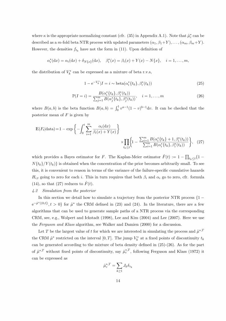
where κ is the appropriate normalizing constant (cfr. (35) in Appendix A.1). Note that µ∗c can be

described as a m-fold beta NTR process with updated parameters (α1, β1+Y ), . . . , (αm, βm+Y ).

However, the densities ftk have not the form in (11). Upon definition of

α∗i (dx) = αi(dx) + δNx(dx), β∗i (x) = βi(x) + Y (x)−Nx, i = 1, . . . ,m,

the distribution of V ∗k can be expressed as a mixture of beta r.v.s,

1− e−V∗k |I = i ∼ beta(α∗i tk, β∗i (tk)) (25)

P(I = i) =B(α∗i tk, β∗i (tk))∑mj=1B(α∗jtk, β∗j (tk))

, i = 1, . . . ,m (26)

where B(a, b) is the beta function B(a, b) =∫ 1

0 va−1(1 − v)b−1dv. It can be checked that the

posterior mean of F is given by

E(Ft|data)=1− exp

−∫ t

0

m∑i=1

αi(dx)

βi(x) + Y (x)

×∏tk≤t

1−

∑mi=1B(α∗i tk+ 1, β∗i (tk))∑mi=1B(α∗i tk, β∗i (tk))

, (27)

which provides a Bayes estimator for F . The Kaplan-Meier estimator F (t) := 1 −∏tk≤t1 −

Ntk/Y (tk) is obtained when the concentration of the prior becomes arbitrarily small. To see

this, it is convenient to reason in terms of the variance of the failure-specific cumulative hazards

Hi,t going to zero for each i. This in turn requires that both βi and αi go to zero, cfr. formula

(14), so that (27) reduces to F (t).

4.2 Simulation from the posterior

In this section we detail how to simulate a trajectory from the posterior NTR process 1−e−µ

∗((0,t]), t > 0 for µ∗ the CRM defined in (23) and (24). In the literature, there are a few

algorithms that can be used to generate sample paths of a NTR process via the corresponding

CRM, see, e.g., Wolpert and Ickstadt (1998), Lee and Kim (2004) and Lee (2007). Here we use

the Ferguson and Klass algorithm, see Walker and Damien (2000) for a discussion.

Let T be the largest value of t for which we are interested in simulating the process and µ∗,T

the CRM µ∗ restricted on the interval [0, T ]. The jump V ∗k at a fixed points of discontinuity tk

can be generated according to the mixture of beta density defined in (25)-(26). As for the part

of µ∗,T without fixed points of discontinuity, say µ∗,Tc , following Ferguson and Klass (1972) it

can be expressed as

µ∗,Tc =∑k≥1

Jkδτk

14

where the random jumps Jk can be simulated in a decreasing order according to their size.

Specifically, let dν∗t (s) = ν∗(ds, (0, t]), then the Jk’s are obtained as solution of the equation

θk = M(Jk), where M(s) = ν∗T ([s,+∞)) and θ1, θ2, . . . are jump times of a standard Poisson

process at unit rate. The random locations τk’s are obtained according to the distribution

function

P(τk ≤ t|Jk) = nt(Jk) where nt(s) =dν∗tdν∗T

(s) (28)

Hence, one can set τk as the solution of uk = nτk(Jk) where u1, u2, . . . are iid from the uniform

distribution on the interval (0, 1), independent of the Jks.

The implementation of the algorithm requires both the calculation of integrals (single in

dν∗t (s) and double in M(s)) and the solution of equations such as θk = M(Jk) and uk = nτk(Jk).

Some devices can be used to avoid, in part, the recourse to numerical subroutines. The measure

dν∗t (s) involves a sum of integrals of the type∫ t

0 e−s[βi(x)+Y (x)]αi(dx) which have closed form for

a prior specification such as in (22) (note that Y (x) is a step function). Then, we can avoid to

solve numerically the equation uk = nτk(Jk) if we write nt(Jk) (the cumulative distribution of

τk|Jk when seen as a function of t, see (28)) in a mixture form as follows

nt(s) =m∑i=1

ωi(s)ni,t(s)

for weights ωi(s) = νi(ds, (0, T ])/∑m

j=1 νj(ds, (0, T ]), νi the Levy intensity of a beta-Stacy pro-

cess of parameter (βi + Y, αi), see (2), and ni,t(s) = νi(ds, (0, t])/νi(ds, (0, T ]). Then, con-

ditionally on I = i, where P(I = i) = ωi(Jk), τk can be generated by solving the equation

uk = ni,τk(Jk), which can be done analytically under the prior specifications (22). As for the

computation of M(s), note that it can be written as

M(s) =

m∑i=1

∫ T

0Be−s(βi(x) + Y (x), 0)αi(dx)

where Bz(a, b) =∫ z

0 sa−1(1 − s)b−1ds denotes the incomplete beta function. Bz(a, 0) can be

computed as the limit of the rescaled tail probabilities of a beta r.v.,

Bz(a, 0) ≈ B(a, ε) · P(Y ≤ z), Y ∼ beta(a, ε) (29)

for ε small. The second integration in M(s) and the solution of the equation θk = M(Jk) needs

to be done numerically.

4.3 Real data example

As an illustrative example, we consider the Kaplan and Meier (1958) data set, already

extensively used by many authors in the Bayesian nonparametric literature. The data consists of

15

the lifetimes 0.8, 1.0∗, 2.7∗, 3.1, 5.4, 7.0∗, 9.2, 12.1∗, where ∗ denotes a right censored observation.

The prior on the random distribution function F is specified by a m-fold beta NTR process with

m = 2 and parameters as in (22) with k1 = k2 = 1 and h0,i(t) = κiλi

(tλi

)κi−1e−(t/λi)

κi , i = 1, 2,

that is two hazard rates of the Weibull type. We choose λ1 = λ2 = 20, κ1 = 1.5 and κ2 = 0.5,

so that the prior process is centered on a survival distribution with non monotonic hazard rate,

see Figure 1.

[Figure 1 about here]

We sample 5000 trajectories from the posterior process on the time interval [0, T ] for T = 50.

In the implementation of the Ferguson and Klass algorithm we set ε = 10−15 in the approx-

imation of Be−s(βi(x) + Y (x), 0), see (29), and we truncate the number of jumps in µ∗,Tc by

keeping only the jumps which induce a relative error in the computation of M smaller than

0.001. It results in a smallest jump of order 2e−15. We evaluate the posterior distribution of the

probability Ft for t = 5 and the exponential-type functional of µ∗,

IT (µ∗) =1

1− e−µ∗((0,T ])

[ ∫ T

0e−µ

∗((0,t])dt− T e−µ∗((0,T ])

]

which corresponds to the random mean of the distribution obtained via normalization of Ft

over [0, T ]. IT (µ∗) can be used to approximate, for T large, the random mean of the posterior

NTR process which takes the interpretation of expected lifetimes. T = 50 can be considered

sufficiently large since direct computation using formula (27) leads to E(FT |data) = 0.996.

The reader is referred to Epifani, Lijoi and Prunster (2003) for a study on the distribution of

the mean of a NTR distribution function where the same data set is used with a beta-Stacy

process prior. Note that the Ferguson and Klass algorithm is not implementable for generating

a trajectory of Ft on the entire positive real axis. In fact, ν∗T ([s,+∞)) → +∞ as T → +∞ for

any s unless the βi functions explode at infinity, which is unlikely to be adopted in applications

where one typically takes decreasing βi’s in order to induce a decreasing concentration of the

prior distribution for large time horizons.

Figure 2(a) displays the histogram and the kernel density estimate of the posterior distribu-

tion of Ft for t = 5 (sample mean 0.3041, sample standard deviation 0.1587), while in Figure

2(b) we compare the density of the distribution of IT (µ∗) with the density of IT (µ), the latter

calculated over 5000 trajectories of the prior process. Sample mean and standard deviation for

IT (µ∗) are 10.7619 and 4.1692, respectively, while IT (µ) has mean 8.9093 and standard deviation

6.2368.

[Figure 2 about here]

16

5 Concluding remarks

In the present paper we have introduced and investigated the properties of a new NTR prior,

named m-fold beta NTR process, for the lifetime distribution which corresponds to the super-

position of independent beta processes at the cumulative hazard level. The use of the proposed

prior is justified in presence of independent competing risks, therefore, it finds a natural area

of application in reliability problems, where such an assumption is often appropriate. The typ-

ical situation is a system consisting of m components that fail independently from each other.

The lifetime of the system is determined by the first component failure, so that the cumulative

hazard results into the sum of the m failure-specific cumulative hazard. The m-fold beta NTR

process allows to specify different prior beliefs for the components’ failure time distribution and

represents a suitable extension of the beta-Stacy process to this setting.

An interesting development consists in studying the case of a system failing when at least

k out of the m components experience a failure (k > 1). The lifetime T of the system would

correspond to the k-th smallest value among the m component failure times X1, . . . , Xm. It is

no more appropriate to model the distribution of T with a NTR process since the conditional

probability of a failure time at t does depend on the past, namely on how many components have

experience a failure up to time t. One can still put independent NTR priors on the distributions

of the Xi’s and study the induced nonparametric prior for the distribution of T . In the simple

case of X1, . . . , Xm iid with common random distribution F , the random distribution of T is

described by the process F(k)t :=

∑mj=k

(mj

)[Ft]

j [1−Ft]m−j . Further work is needed to establish

the existence of the corresponding nonparametric prior.

Future work will also focus on adapting the idea of superposition of stochastic processes

at the cumulative hazard level into a regression framework. The goal is to provide a Bayesian

nonparametric treatment of the additive regression model of Aalen (1989), which specifies the

hazard rate of an individual with covariate vector z = (z1, . . . , zp) as the sum h(t, z) = h0(t) +

γ1(t)z1 + . . . + γp(t)zp, for h0 a baseline hazard and γi’s the regression functions. There are

two main issues to address this task. First, the shapes of the regression functions γi’s are left

completely unspecified, therefore they are not constrained to define proper hazards. Secondly,

the nonparametric prior on h0 and γi can not be taken as independent because of the restriction

imposed by h(t, z) ≥ 0. Work on this is ongoing.

Appendix

A.1 NTR priors and CRMs

Here we review some basic facts on the connections between NTR priors and CRMs. The

17

reader is referred to Lijoi and Prunster (2008) for an exhaustive account. Denote by M the

space of boundedly finite measures on B(R+) (that is µ in M has µ((0, t]) < ∞ for any fi-

nite t) endowed with the Borel σ-algebra M . A CRM µ on B(R+) is a measurable mapping

from some probability space (Ω,F ,P) into (M,M ) and such that, for any collection of disjoint

sets A1, . . . , An in B(R+), the r.v.s µ(A1), . . . , µ(An) are mutually independent. This entails

that the random distribution function induced by µ, namely µ((0, t]), t ≥ 0, is an indepen-

dent increment process. CRMs are discrete measures with probability 1 as they can always be

represented as the sum of two components:

µ = µc +M∑k=1

Vkδxk (30)

where µc =∑

i≥1 JiδXi is a CRM where both the positive jumps Ji’s and the locations Xi’s are

random, and∑M

k=1 Vkδxk is a measure with random masses V1, . . . , VM , independent from µc, at

fixed locations x1, . . . , xM . Finally, µc is characterized by the Levy-Khintchine representation

which states that

E

[e−

∫R+

f(x)µc(dx)]

= exp

−∫R+×R+

[1− e−sf(x)

]ν(ds, dx)

(31)

where f is a real-valued function µc-integrable almost surely and ν, referred to as the Levy

intensity of µc, is a nonatomic measure on R+ × R+ such that∫B

∫R+

mins, 1ν(ds, dx) < ∞for any bounded B in B(R+).

As pointed out by Doksum (1974), a random distribution function F is NTR (see definition

in (1)) if and only if

Ft = 1− e−µ((0,t]), t ≥ 0

for some CRM µ on B(R+) such that P[limt→∞ µ((0, t]) = ∞] = 1. We will use the notation

F ∼ NTR(µ). A consequence of this characterization is that, by using (31), the expected value

of Ft is expressed in terms of the Levy intensity ν of µ (no fixed jumps case) as

E[Ft] = 1− E[e−µ((0,t])

]= 1− exp

−∫ t

0

∫ ∞0

(1− e−s)ν(ds, dx). (32)

A second characterization of NTR prior in terms of CRMs arise while assessing the prior

distribution induced by F on the space of cumulative hazards, see Hjort (1990). Let F ∼ NTR(µ)

for a CRM µ without fixed jumps and let ν(ds, dx) = ν(s, x)ds dx (with a little abuse of notation)

be the corresponding Levy intensity. The random cumulative hazard H(F ), see (3), is given by

Ht(F ) =

∫ t

0

dFx1− Fx−

= η((0, t]), t ≥ 0

18

where η is a CRM with Levy intensity νH(dv,dx) = νH(v, x)dv dx such that νH(v, x) = 0 for

any v > 1. The conversion formula for deriving the Levy intensity of η from that of µ is as

follows:

νH(v, x) =1

1− vν(− log(1− v), x), (v, x) ∈ [0, 1]×R+ (33)

that is νH(dv,dx) is the distribution of (s, x) 7→ (1 − e−s, x) under ν, see Dey, Erickson and

Ramamoorthi (2003).

Consider now an exchangeable sequence of lifetimes (Xi)i≥1 such that the law of the sequence

is directed by a NTR process F for some CRM µ,

Xi|Fiid∼ F i ≥ 1 F ∼ NTR(µ)

We derive the posterior distribution of F given X1, . . . , Xn subject to censoring times c1, . . . , cn,

which can be either random or non–random. The actual data consist in the observed lifetimes

Ti = min(Xi, ci) and the censoring indicators ∆i = 1(Xi≤ci). Define N(t) =∑

i≤n 1(Ti≤t,∆i=1)

and Y (t) =∑

i≤n 1(Ti≥t), where N(t) counts the number of events occurred before time t and

Y (t) is equal to the number of individuals at risk at time t.

Theorem 5.1 (Ferguson and Phadia (1979)). Suppose F ∼ NTR(µ) where µ has no fixed jump

points. Then the posterior distribution of F , given

(T1,∆1), . . . , (Tn,∆n) is NTR(µ∗) with

µ∗ = µ∗c +∑

k:Ntk>0 V∗k δtk

where µ∗c is a CRM without fixed jump points and it is independent of the jumps V ∗k ’s, which

occur at the exact observations.

Let ν(ds, dx) = ρx(s)ds α(dx) be the Levy intensity of µ. Then the Lvey measure ν∗ of µ∗c is

given by

ν∗(ds, dx) = e−sY (x)ρx(s)ds α(dx) (34)

whereas the density of the jump V ∗k at time point tk is given by

ftk(s) =(1− e−s)Ntke−s[Y (tk)−Ntk]ρtk(s)∫∞

0 (1− e−u)Ntke−u[Y (tk)−Ntk]ρtk(u)du. (35)

A.2 Proof of Theorem 2.1.

Following the lines of the proof of Theorem 2 in Walker and Muliere (1997) we define, for

any integer n, m sequences of positive real numbers (α(n)1,• , β

(n)1,• ), . . . , (α

(n)m,•, β

(n)m,•) such that

α(n)i,k := αi

(k − 1

n,k

n

], β

(n)i,k := βi

(k

n− 1

2n

)19

for i = 1, . . . ,m and for any k ≥ 1. Moreover, let us consider m independent sequences

Y(n)

1,• , . . . , Y(n)m,• such that Y

(n)i,• is a sequence of independent r.v.s with Y

(n)i,k ∼ beta(α

(n)i,k , β

(n)i,k ).

Based on this setup of r.v.s, for any n we define the random process Z(n) := Z(n)t , t ≥ 0 as

Z(n)t := −

∑k/n≤t

log

(1−

X(n)k

1− F (n)k−1

)

with Z(n)0 := 0 and X(n)

k , k ≥ 1 a sequence of r.v.s defined according to (5).

The first step consists in showing that the sequence of random processes Z(n)t , t ≥ 0n≥1

converges weakly to the process µ((0, t]), t ≥ 0 for µ the CRM having Levy intensity in (7).

Let Γ(x) =∫∞

0 yx−1e−ydy be the gamma function. By using the recursive relation Γ(x) =

(x− 1)Γ(x− 1) and the Stirling formula Γ(x) ∼= (2πx)1/2(x/e)x when x is large, we have

log(E[e−φZ(n)t ]) = log

(E[e−φ

∑k/n≤t

∑mi=1− log(1−Y (n)

i,k )])

=∑k/n≤t

m∑i=1

logΓ(α

(n)i,k + β

(n)i,k )Γ(β

(n)i,k + φ)

Γ(β(n)i,k )Γ(α

(n)i,k + β

(n)i,k + φ)

=∑k/n≤t

m∑i=1

logr−1∏j=0

(β(n)i,k + j)(α

(n)i,k + β

(n)i,k + φ+ j)

(α(n)i,k + β

(n)i,k + j)(β

(n)i,k + φ+ j)

Γ(α(n)i,k + β

(n)i,k + r)Γ(β

(n)i,k + φ+ r)

Γ(β(n)i,k + r)Γ(α

(n)i,k + β

(n)i,k + φ+ r)

=∑k/n≤t

m∑i=1

log∏j≥0

(β(n)i,k + j)(α

(n)i,k + β

(n)i,k + φ+ j)

(α(n)i,k + β

(n)i,k + j)(β

(n)i,k + φ+ j)

=∑k/n≤t

m∑i=1

∫ +∞

0(e−φs − 1)

e−β(n)i,k s(1− e−α

(n)i,k s)

s(1− e−v)ds

=

∫ +∞

0

e−φs − 1

s(1− e−s)

∑k/n≤t

m∑i=1

e−β(n)i,k s(1− e−α

(n)i,k s)ds.

Since for i = 1, . . . ,m, as n→ +∞,∑k/n≤t

e−β(n)i,k s(1− e−α

(n)i,k s)→ s

∫ t

0e−sβi(x)αi(dx),

one has that, as n→ +∞,

log(E[e−φZ(n)t ])→

∫ +∞

0

e−φs − 1

1− e−s

m∑i=1

∫ t

0e−sβi(x)αi(dx)ds.

This result ensures the convergence of the finite dimensional distributions of Z(n)t , t ≥ 0

to those of µ((0, t]), t ≥ 0, cfr. Levy-Khintchine representation (31). The tightness of the

sequence (Z(n))n≥1 follows by the same arguments used in Walker and Muliere (1997).

20

For any n ∈ N, let us define the discrete time m-fold beta NTR process F (n)t , t ≥ 0 such

that F(n)t :=

∑k/n≤tX

(n)k with F

(n)0 = 0. Since

− log(1− F (n)t ) = −

∑k/n≤t

log

(m∏i=1

(1− Yi,k)

)= −

∑k/n≤t

log

(1−

X(n)k

1− F (n)k−1

)= Z

(n)t

then F(n)t = 1 − eZ

(n)t . Note that, for t = k/n, F

(n)t− = F

(n)(k−1)/n and dF

(n)t := F

(n)t+dt − F

(n)t− is

given by F(n)k/n − F

(n)(k−1)/n for dt small, where

F(n)k/n − F

(n)(k−1)/n

∣∣F (n)(k−1)/n

d=(1− F (n)

(k−1)/n

)(1−

∏mi=1(1− Y (n)

i,k )).

The same arguments used when taking the limit above yields, at the infinitesimal level, dFt|Ftd=

(1 − Ft−) (1−∏mi=1(1− Yi,t)) where Ft = 1 − e−µ((0,t]) and Y1,t, . . . , Ym,t are independent r.v.s

such that Yi,t ∼ beta(αi(dt), βi(t)). The fact that Ft, t ≥ 0 defines a random distribution

function is assured by E[Ft] → 0 as t → +∞, which can be checked by using (32) under the

hypothesis on∫ t

0

∑mi=1 βi(x)−1αi(dx) since E[1−Ft] = exp−

∫ t0

∑mi=1 βi(x)−1αi(dx). It follows

that Ft, t ≥ 0 is a NTR process according to definition (1), which completes the proof.

Acknowledgements

The authors are grateful to Fabrizio Ruggieri for a useful discussion. This work is partially

supported by MIUR grant 2008MK3AFZ.

References

[1] Aalen, O.O. (1989). A linear regression model for the analysis of life times. Stat. Med. 8,

907–925.

[2] Andersen, P.K., Borgan, Ø., Gill, R.D. and Keiding, N. (1993). Statistical models based on

counting processes. Springer, New York.

[3] Connor, R. J. and Mosimann, I. E. (1969). Concepts of independence for proportions with

a generalization of the Dirichlet distribution. J. Amer. Statist. Assoc. 64, 194-206.

[4] Dey, J., Erickson, R.V. and Ramamoorthi, R.V. (2003). Some aspects of neutral to the

right priors. Internat. Statist. Rev. 71, 383–401.

[5] Doksum, K. A. (1974). Tailfree and neutral random probabilities and their posterior distri-

butions. Ann. Probab. 2, 183–201.

21

[6] Epifani, I., Lijoi, A., Prunster, I. (2003). Exponential functionals and means of neutral-to-

the-right priors. Biometrika 90, 791–808.

[7] Erdelyi, A., Magnus, W., Oberhettinger, F., and Tricomi, F. G. (1976). Higher trascenden-

tal functions Vol. I. McGraw-Hill, New York.

[8] Ferguson, T. S. (1974). Prior distributions on spaces of probability measures. Ann. Statist.

2, 615–629.

[9] Ferguson, T. S., Phadia, E. G. (1979). Bayesian nonparametric estimation based on cen-

sored data. Ann. Statist. 7, 163–186.

[10] Ferguson, T. S., Klass, M. J. (1972). A representation of independent increment processes

without Gaussian components. Ann. Math. Statist. 43, 1634–1643.

[11] Hjort, N. L. (1990). Nonparametric Bayes estimators based on Beta processes in models for

life history data. Ann. Statist. 18, 1259–1294.

[12] Jambunathan, M.V. (1954). Some properties of beta and gamma distributions. Ann. Math.

Stat. 25, 401–405.

[13] James, L. F. (2006). Poisson calculus for spatial neutral to the right processes. Ann. Statist.

34, 416–440.

[14] Kaplan, E.L., Meier, P. (1958). Nonparametric estimation from incomplete observations. J.

Am. Statist. Assoc. 53, 457–481.

[15] Kim, Y., Lee, J. (2001). On posterior consistency of survival models. Ann. Statist. 29, 666–

686.

[16] Kim, Y., Lee, J. (2004). A Bernstein-von Mises theorem in the nonparametric right-

censoring model. Ann. Statist. 32, 1492–1512.

[17] Lee, J. (2007). Sampling methods for neutral to the right processes. J. Comput. Graph.

Statist. 25, 401–405.

[18] Lee, J., Kim, Y. (2004). A new algorithm to generate beta processes. Comput. Statist. Data

Anal. 25, 401–405.

[19] Lijoi, A., Prunster, I. (2008). Models beyond the Dirichlet process. In Bayesian Nonpara-

metrics (Eds. N.L. Hjort, C.C. Holmes, P. Muller and S.G. Walker). Cambridge University

Press, in press.

22

[20] Springer, M.D., Thompson, W.E. (1970). The distribution of products of Beta, Gamma and

Gaussian random variables. SIAM J. Appl. Math. 18, 721–737.

[21] Walker, S.G. and Damien P. (2000). Representation of Levy processes without Gaussian

components. Biometrika 87, 477–483.

[22] Walker, S. G., Muliere, P. (1997). Beta-Stacy processes and a generalization of the Polya-

urn scheme. Ann. Statist. 25, 1762–1780.

[23] Wilks, S.S. (1932). Certain generalizations in the analysis of variance. Biometrika. 24, 471–

494.

[24] Wolpert, R. L., Ickstadt, K. (1998). Simulation of Levy random fields. In Practical Non-

parametric and Semiparametric Bayesian Statistics (Eds. D. Dey, P. Muller and D. Sinha),

volume 133 of Lecture Notes in Statistics. Springer, New York, 227–242.

23

0 10 20 30 40 50

0.00

0.05

0.10

0.15

0.20

0.25

Time

Haz

ard

rate

(a)

0 10 20 30 40 50

01

23

45

Time

Cum

ulat

ive

haza

rd

(b)

Figure 1: (a) Hazard rate (—) and failure-specific hazard rates h0,1 (- - -) and h0,2 (-·-·-) in the

prior. (b) The same for the cumulative hazard.

Ft

dens

ity

(a)

0.0 0.2 0.4 0.6 0.8 1.0

0.0

0.5

1.0

1.5

2.0

2.5

0 10 20 30 40

0.00

0.02

0.04

0.06

0.08

0.10

0.12

Time

dens

ity

(b)

Figure 2: (a) Histogram and density estimates of the posterior distribution of Ft for t = 5. (b)

Density estimate of IT (µ∗) (—) and IT (µ) (- - -) for T = 50; sample mean and sample s.d. of

IT (µ∗)

24