JOURNAL OF MULTIVARIATE ANALYSIS 25, 25-30 (1988)

A Characterization of Dirichlet Distributions

B. V. RAO AND BIKAS K. SINHA*

Indian Statistical Institute, Calcutta, India

Communicated by C. G. Khatri

J. N. Darroch and D. Ratcliff (J. Amer. Statist. Assoc. 66 (1971), 641643) have given a characterization of the Dirichlet distributions based on the properties of independence of various functions of the random variables (X,, X,, . . . . X,) having a joint continuous distribution over the k-dimensional simplex: 0 < x, <x x, < 1. In this paper we provide a further characterization of this family of distributions essen- tially based on the properties of linear regression. Some extra conditions have been imposed and these are indeed indispensable. 0 1988 Academic Press. Inc.

1. INTRODUCTION

Characterizations in statistics form a fascinating area of study and research. There is a huge literature on characterizations of statistical distributions based on various properties of such distributions. This paper aims at incorporating a characterization of the Dirichlet family of dis- tributions based on the properties of regression. The motivation came from a recent work [2] in which Neyman’s problem of characterization of the family of multinomial distributions based on the properties of regression was properly studied and the present problem posed.

In [l], a characterization of the Dirichlet family of distributions is available. Note that a two-dimensional random variable (X, Y) is said to have Dirichlet distribution if the joint density f(x, y) is of the form

fi,8,y(~,y)=Const.xa-1yB-1(l-x-y)~~1;

a,~,y>O;O<x,y<x+y<l. (1.1)

For the two-dimensional case, the result in [l] may be stated as follows:

Received November 26, 1984; revised January 7, 1987. AMS 1980 subject classifications: primary 62El0, secondary 62505. Key words and phrases: Dirichlet distributions, linearity of regression. * Currently visiting the Department of Mathematics. Statistics and Computer Science,

University of Illinois, Chicago, IL 60680.

25 0047-259X/88 $3.00

Copyright 0 1988 by Academic Press, Inc. All rights of reproduction in any form reserved.

26 RAOANDSINHA

Suppose (X, Y)-f(x, y) over the simplex O<x, y<?c+ y< 1. Assume f(x, y), f(x, .), and f( ., y) (the marginals) to be continuous. Then (X, Y) N Dirichlet iff the following two conditions hold simultaneously:

(a) (X/( 1 - Y), Y) are independently distributed,

(b) ( Y/( 1 - X), X) are independently distributed.

Clearly, for the Dirichlet distribution (l.l),

E(XI Y) =- a;y(l- n E(w)=B+v P(l -X). (1.2)

The present investigation arose in trying to characterize the Dirichlet dis- tribution through the regression equations alone. Obviously, the two linear equations by themselves are not strong enough to characterize the Dirichlet (see Remarks 1 and 2). The extra conditions needed are that the density be of the product form and one of these terms be a power function. These conditions seem too strong but in spite of these, the proof that the density must be Dirichlet turns out to be interesting. That these conditions are the best possible is shown by Remark 2.

2. SOME PRELIMINARY RESULTS

LEMMA 1. Let X, Y be jointly distributed with law P having full support on the simplex 0 < x, y, x + y < 1. Assume that the two regressions E(X( Y) and E( Y ( X) are linear. Then there exist constants 0 < c < 1, 0 < d < 1 such that

E(X( Y) = c( 1 - Y) a.e. [Y]

E(YlX)=d(l-X) a.e. [Xl.

Proof: Assume that E(XI Y)=a( I- Y)+ /I so that 0 < a(1 - Y) + /3 < 1 - y a.e. [PI. Since the support of P is the full simplex, take { yn} --f 1 such that for each y, this inequality holds. This gives p =O. It is now immediate that 0 < a < 1. This completes the proof.

LEMMA 2. Let 4 be a positive integrable function on (0, 1). Suppose that

J b’(Y4 “+‘d(t)dt=cyJY(y-t)a&t)dt forall y~(O,l), 0

where 0 CC < 1, a > -1 and the integral on the right-hand side exists. Then $(t) = cotY-’ for alf t E (0, l), co is a constant, and q = (a + l)( 1 -c) > 0.

DIRICHLET DISTRIBUTIONS 27

Proof. Let ~(y)=joY(~-t)“l~(t)dt. Then J/‘(y)=(a+l) j,‘(y--t)“&t)dt and taking cl = (tl + 1)/c, the given equation can be written as

Hence

V(YMY) = Cl/Y

$(Y) = co YC’

for all y E (0, 1).

for all y E (0, 1 ),

where c0 is some constant of integration. Then, we can write

j~(z-y)"-1(j~(y-l)"m(t)dl)dy=(c&)j~(z-y)6-' y"'-'dy

for all z E (0, 1) and for all 6 > 0. After interchanging the integrations of t and y, we can write

(y-tydy dt=(CO/C)z6+c’--B(6,cl)

Or

f 1(1-t)“+~~(1Z)dt=(co/c)z~-1B(P+6+1,y)/B(a+1,Y)

0

for all z E (0, 1) and y = cI - CI - 1 ( >O). This gives Mellin’s transform of t”#( (1 - r)), namely,

s ‘r~{r~~((l-t)2)~dt=(co/c)~Y~1B(a+6+~,y)/B(~+1,y),

0

and then using the uniqueness of Mellin’s transformation, we get the required result. This proves Lemma 2.

3. MAIN RESULTS: TWO-DIMENSIONAL CASE

THEOREM 1. Let (X, Y) be a random vector having joint distribution over the simplex S = { 0 < x, y, x + y < 11 with density function f (x, y ). Assume that

6) fk y)>Ofor all k y)ES;

6) f(x, y)=fl(x)f2(y)f3(1 -x-v)for all (x2 Y)ES;

(iii) f, or f3 is a power function; and

(iv) regression of X on Y is linear.

28 RAOANDSINHA

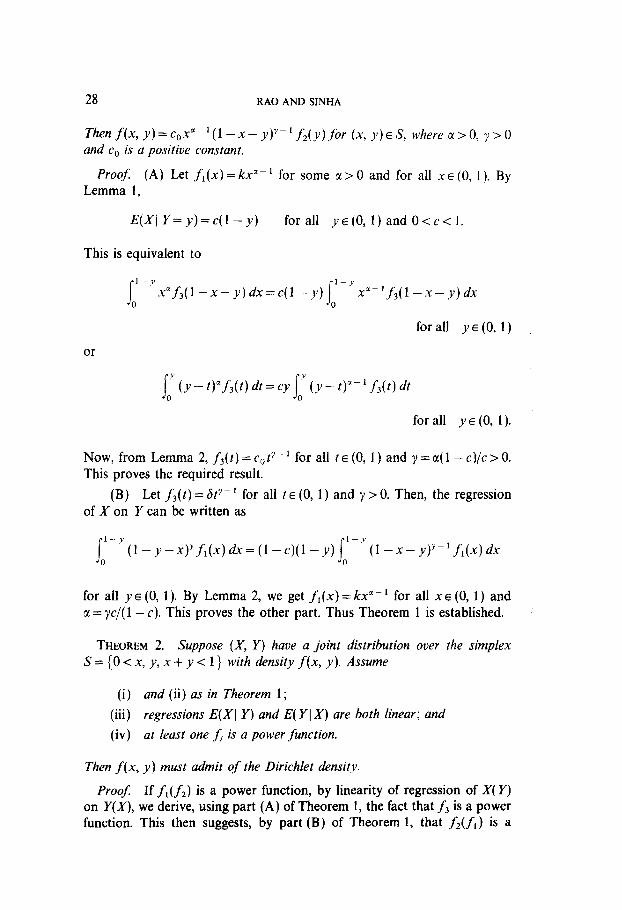
Then f(x, y) = cOxa ~ ’ (1 - x - y)‘~ ’ f*(y) for (x, y) E S, where a > 0, y > 0 and c0 is a positive constant.

Proof (A) Let f,(x) = kx”- ’ for some c( > 0 and for all x E (0, 1). By Lemma 1.

E(XI Y=y)=c(l-JJy) forall yE(O,l)andO<c<l.

This is equivalent to

id--‘xCf3(l-x-y)dx=c(l-g) j;-‘x2-‘f3(l-x+x

for all YE (0, 1)

or

1’ ; (y-t)OLf3(t)dt=cy s o (Y-V-'f&W

for all yE (0, 1).

Now, from Lemma 2, f3(t) = c,ty- ’ for all t E (0, 1) and y = a( 1 - c)/c > 0. This proves the required result.

(B) Let f3(t)=BtY-’ for all t E (0, 1) and y >O. Then, the regression of X on Y can be written as

I ‘-y(l-y-x)yf,(x)dx=(l-~)(l-y)jd-i(l-x-y)’-’f,(x)dx 0

for all y E (0, 1). By Lemma 2, we get fr (x) = kx” ~ ’ for all x E (0, 1) and a = yc/( I- c). This proves the other part. Thus Theorem 1 is established.

THEOREM 2. Suppose (X, Y) have a joint distribution over the simplex S = { 0 < x, y, x + y < 1) with density f (x, y ). Assume

(i ) and (ii) as in Theorem 1;

(iii) regressions E(XI Y) and E( Y 1 X) are both linear; and (iv) at least one f, is a power function.

Then f(x, y) must admit of the Dirichlet density.

Proof: If fi(fi) is a power function, by linearity of regression of X(Y) on Y(X), we derive, using part (A) of Theorem 1, the fact that f3 is a power function. This then suggests, by part (B) of Theorem 1, that f2(f,) is a

DIRICHLET DISTRIBUTIONS 29

power function since linearity of regression of Y(X) on X(Y) is also assumed here. This essentially proves the result.

Remark 1. Unless f(x, y) is of the product form (ii), we do not have the CharacterizationThis is seen through the following example. Recall that

where G.,, is a normalizing constant. Here, as always below, CC > 0, j > 0, y~O.Fixsuchana,~,y.Fixk#l,k~O.FixO~p~landq=l-p.Put

f(X? .Y) = Pf,,pJx? y) + qf/cN?.ky(x7 Y).

Then f(x, y) is a density for which conditions (i) and (iii) of Theorem 2 hold. But f(x, y) is not of the product form and f(x, y) is not Dirichlet. Actually, we can take any nondegenerate probability I7 on (0, co) and define

Ax, Y) = Iorn fwcg.ky(x> Y) dn(k).

Remark 2. Unless one of the fi’s is a power function, we may again come up with a counterexample as is shown below.

Take any positive continuous function 6 on [O, I], e.g., 6(x) = x + x2. Put f(x, y) = kS(x) 6(y) 6( 1 - x - y), where k is a normalizing constant. Assuming that S > 0 a.e., we see that f(x, y) satisfies conditions (i) and (ii) of either theorem. We shall verify that both regressions are indeed linear. If jg x6(x) S(y - x) dx = LX, then changing x to y - x and adding the resulting equation to this, we get

or

That is, E(XI Y = y) = (1 - y)/2. By symmetry, the other regression is also linear. However, f(x, y) is not

Dirichlet unless 6(x) is a power function. Of course, here, though f (x, y) is of the product form, none of the f;s is a power function.

Remark 3. We have not been able to give a nice statistical inter- pretation to condition (iv) of Theorem 2.

30 RAOANDSINHA

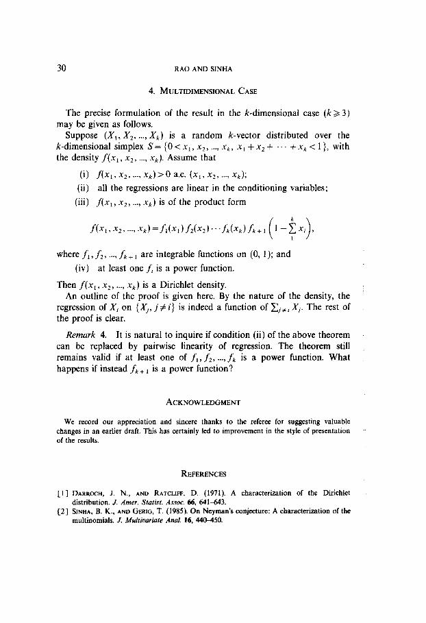
4. MULTIDIMENSIONAL CASE

The precise formulation of the result in the k-dimensional case (k z 3) may be given as follows.

Suppose (X,, X2, . . . . X,) is a random k-vector distributed over the k-dimensional simplex S = (0 < x1, x2, . . . . xk, x, + x2 + . . . + xk < 1 }, with the density j-(x,, x2, . . . . xk). Assume that

(i) fb,, x2, . . . . xk) > 0 a.e. (x,, x2, . . . . x,);

(ii) all the regressions are linear in the conditioning variables;

(iii) f(xr , x2, . . . . xk) is of the product form

f&l 9 x2 9 . . . . xk)=~~(x,)fZ(x~)“‘fk(xk)fk+,

where h, f2, . . . . fk + , are integrable functions on (0, 1); and

(iv) at least one fi is a power function.

Then f(x,, x2, . . . . xk) is a Dirichlet density. An outline of the proof is given here. By the nature of the density, the

regression of Xi on {Xi, j# i} is indeed a function of cj+ i X,. The rest of the proof is clear.

Remark 4. It is natural to inquire if condition (ii) of the above theorem can be replaced by pairwise linearity of regression. The theorem still remains valid if at least one of fr, f2, . . . . fk is a power function. What happens if instead fk+ r is a power function?

ACKNOWLEDGMENT

We record our appreciation and sincere thanks to the referee for suggesting valuable changes in an earlier draft. This has certainly led to improvement in the style of presentation of the results.

REFERENCES

[l] DARROCH, J. N., AND RATCLIFF, D. (1971). A characterization of the Dirichlet distribution. J. Amer. Statist. Assoc. 66, 64143.

[Z] SINHA, B. K., AND GERIG, T. (1985). On Neyman’s conjecture: A characterization of the multinomials. J. h4ultioariate Anal. 16, 440450.