a central california coastal ocean modeling study: 1...

A central California coastal ocean modeling study:

1. Forward model and the influence of realistic versus

climatological forcing

M. Veneziani,1 C. A. Edwards,1 J. D. Doyle,2 and D. Foley3

Received 14 February 2008; revised 3 September 2008; accepted 22 January 2009; published 25 April 2009.

[1] We report on a numerical simulation of the California Current circulation using theRegional Ocean Modeling System model, focusing on the region of northern andcentral California during the 5-year period from 2000 to 2004. Unlike previous modelstudies of the California Current System, the present configuration is characterized by bothrealistic external forcing and a spatial domain covering most of the North AmericanWest Coast. Specifically, this configuration is driven at the surface by high-resolutionmeteorological fields from the Coupled Ocean-Atmosphere Mesoscale Prediction Systemand at the lateral open boundaries by output from the project Estimating theCirculation and Climate of the Ocean supported by the Global Ocean Data AssimilationExperiment. The simulation is evaluated favorably through quantitative comparisonswith the California Cooperative Fisheries Investigations data set, satellite-derivedsea surface temperature, and surface drifters–derived eddy kinetic energy. The impact ofadopting realistic versus climatological surface forcing is demonstrated by comparingmean and mesoscale circulation characteristics. Realistic surface forcing qualitativelyalters the seasonal cycle of the mean alongshore jet and better reproduces the summerspatial structure and intensity of the eddy kinetic energy field along the centralCalifornia coast.

Citation: Veneziani, M., C. A. Edwards, J. D. Doyle, and D. Foley (2009), A central California coastal ocean modeling study:

1. Forward model and the influence of realistic versus climatological forcing, J. Geophys. Res., 114, C04015,

doi:10.1029/2008JC004774.

1. Introduction

[2] The California Current is a typical eastern boundarycurrent whose coastal dynamics are directly tied to theatmospheric wind forcing and highly influenced by thesteep bathymetry, narrow continental shelf, and shape ofthe coastline. Its circulation has been widely studied throughobservational efforts [e.g., Rosenfeld et al., 1994; Swensonand Niiler, 1996; Ramp et al., 1997; Barth et al., 2000;Strub and James, 2000] and numerical modeling [e.g.,McCreary et al., 1987; Batteen, 1997; Gan and Allen,2002a, 2002b; Marchesiello et al., 2003; J. M. Pringleand E. P. Dever, Dynamics of wind-driven upwelling andrelaxation between Monterey Bay and Pt. Arena: Local,regional and gyre scale controls, submitted to Journal ofGeophysical Research, 2009]. The California Current Sys-tem (CCS) is composed of the wind-driven, broad, weakequatorward flow found offshore, and a coastal flow whosespatial and temporal characteristics are subject to the strong

seasonal cycle induced by changes in the atmosphericpressure field (excellent reviews of the CCS can be foundin the papers by Hickey [1979, 1998]). In winter, theAleutian low-pressure system is well established over theGulf of Alaska, producing predominantly west-southwest-erly winds along the Washington and Oregon coast, inshoreEkman transport, and consequent downwelling conditions.To the south, the North Pacific high-pressure system gen-erally occupies a vast area over most of the North PacificOcean, causing northwesterly winds along the Californiaand Mexico coast south of Cape Mendocino (key geograph-ical locations are indicated in Figure 1), and upwellingconditions year-round. In winter, however, the strengthen-ing of the Aleutian low occurs, while the North Pacific highshifts to the south, thus weakening considerably the centralCalifornia coastal northwesterly winds and associated up-welling circulation. During the so-called ‘‘spring transition’’[Lynn et al., 2003], the Aleutian low retreats northward, theNorth Pacific high strengthens and northwesterly windsextend uninterruptedly along the North American WestCoast south of Washington. These events mark the start ofthe upwelling season in the ocean with the formation of astrong, surface intensified, coastal equatorward jet. As theseason progresses, the coastal jet evolves from a narrowfeature tightly hugging the coastline to a highly meanderingstructure, with standing meanders extending several hun-

JOURNAL OF GEOPHYSICAL RESEARCH, VOL. 114, C04015, doi:10.1029/2008JC004774, 2009ClickHere

for

FullArticle

1Ocean Sciences Department, University of California, Santa Cruz,California, USA.

2Naval Research Laboratory, Monterey, California, USA.3Environmental Research Division, NOAA Southwest Fisheries

Science Center, Pacific Grove, California, USA.

Copyright 2009 by the American Geophysical Union.0148-0227/09/2008JC004774$09.00

C04015 1 of 16

http://dx.doi.org/10.1029/2008JC004774

dred kilometers offshore in correspondence of the majorcoastal promontories (from north to south: Cape Blanco,Cape Mendocino, Point Arena, Point Sur, Point Concep-tion). Internal instabilities of the meandering jet cause theformation of eddies and filaments during the summer andearly fall season [e.g., Chereskin et al., 2000; Strub andJames, 2000; Marchesiello et al., 2003]. Finally, in the fall,when the Aleutian low-pressure system strengthens and thewinds along the California coast weaken, coastal upwellingis reduced considerably and the equatorward jet is replacedby a coastal poleward flow, often called the DavidsonCurrent.[3] While this broad picture of the CCS circulation is well

established, several open questions remain about the detailsof its variability and forcing, particularly on the extent oflocal versus remote driving mechanisms [Davis and Bogden,1989; Hickey et al., 2003, 2006], and on the physics andvariability of the subsurface and deep circulation on thecontinental shelf and slope [Werner and Hickey, 1983;Collins et al., 2000; Noble and Ramp, 2000; Pierce et al.,2000]. In this and a companion paper [Veneziani et al., 2009](hereinafter referred to as part 2), we address some of thesequestions by investigating the sensitivity of the centralCalifornia coastal circulation to the local external forcingand internal dynamics versus the large-scale and remoteforcing mechanisms. Our methodology is to perform a high-resolution modeling study of the CCS using the RegionalOcean Modeling System (ROMS) model. In part 2, we carryout sensitivity studies using the adjoint model approach bytaking advantage of the powerful tangent-linear and adjointmodules recently developed for ROMS [Moore et al., 2004].In the present paper, the objective is twofold. First, we intendto present the results of the ROMS forward simulation (werefer to ‘‘forward’’ simulation when describing the fullnonlinear ROMS model results, whereas ‘‘adjoint’’ refersto the backward in time adjoint model simulation), which

differs from other model studies of the California Currentregion in the application of realistic forcing over a spatialdomain covering most of the U.S. West Coast. Indeed,former investigations are either realistic but local [e.g.,Gan and Allen, 2002b; Shulman et al., 2002; Di Lorenzo,2003; Cervantes and Allen, 2006; Shulman et al., 2007] orextend over a large domain but adopt climatological externalforcing data [e.g.,Marchesiello et al., 2003]. Second, we aimat assessing the importance of adopting realistic externalforcing versus climatological fields to determine the struc-ture of the CCS circulation. At this scope, we performtraditional sensitivity analyses by changing the type ofproduct used as surface and lateral boundary conditions(BCs), and by observing the impact on metrics representa-tive of both the mean and mesoscale circulation. The resultsare quite revealing for they show that the realistic surfaceforcing better reproduces not only key features of the meanalongshore jet along the U.S. West Coast, but also theintensity of its mesoscale structures in proximity of the maincoastal promontories.[4] The paper is organized as follows. The model con-

figuration is described in section 2, while the simulatedcirculation and a comparison with observations are pre-sented in section 3. The results of the sensitivity studies tothe type of external forcing are described in section 4, and adiscussion of the conclusions of this paper is included insection 5.

2. Regional Ocean Modeling System

[5] ROMS is a primitive equation, hydrostatic, freesurface ocean general circulation model [Shchepetkin andMcWilliams, 2005], which has been widely used forregional and coastal ocean applications [e.g., Di Lorenzo,2003; Capet et al., 2004; Cervantes and Allen, 2006;Doglioli et al., 2006; Wilkin and Zhang, 2007; J M Pringleand E P Dever, submitted manuscript, 2009] as well aslarge-scale studies [e.g., Marchesiello et al., 2003; Wangand Chao, 2004; Curchitser et al., 2005; Gruber et al.,2006]. Its terrain-following s-coordinate scheme isdesigned to provide higher vertical resolution near theocean surface and bottom, where small-scale, turbulentdynamics occur and the influence of topographic featuresis greatest [Song and Haidvogel, 1994; Haidvogel et al.,2000; Shchepetkin and McWilliams, 2005].[6] The ROMS configuration chosen for the present study

(Figure 1) covers a large domain extending zonally from134�W to 115.5�Wand meridionally from Washington State(48�N) to northern Baja California (30�N). It features a 1/10�horizontal resolution and 42 s-levels. The vertical resolutionvaries spatially and is equal to �0.3–8 m over the conti-nental shelf, while ranging offshore between 7 m at thesurface and 300 m in the deep ocean. The model topographyis obtained by bicubic interpolation of the ETOPO2 analysis[Amante and Eakins, 2001] and by using a Shapiro filter tosmooth depth gradients such that jd hj/2h < 0.35 (where h =depth). This is a common practice used in terrain-followingcoordinate models to avoid large errors in the pressuregradient computation [Haney, 1991].[7] The data used to constrain the circulation at the three

open boundaries of the domain is provided by the Estimat-ing the Circulation and Climate of the Ocean project

Figure 1. Spatial domain and topography of the presentROMS configuration. Contour lines are every 500 m depth.Thick black lines indicate the three cross-shore sections forwhich vertical profiles of alongshore currents are considered(see section 3.2 and Figures 8 and 11).

C04015 VENEZIANI ET AL.: CCS SENSITIVITY TO EXTERNAL FORCING

2 of 16

C04015

[Wunsch and Heimbach, 2007; Wunsch et al., 2007], whichhas been developed in the framework of the Global OceanData Assimilation Experiment, and is therefore commonlyreferred to as ECCO-GODAE. It is based on the global,z-level, primitive equation Massachusetts Institute of Tech-nology General Circulation Model (MITgcm) [Marshall etal., 1997a, 1997b], featuring a 1� horizontal resolution and23 vertical levels. ECCO-GODAE employs an adjoint-based assimilation technique to assimilate a variety ofglobal observations, such as WOCE hydrography, satellitealtimetry data, and ARGO floats.[8] In order to build the necessary ROMS boundary

conditions, the ECCO-GODAE product is interpolated fromz- to s-level coordinates: a bilinear interpolation is used forfree surface, h, temperature, T, and salinity, S, while abicubic scheme is adopted for the horizontal velocity field,u, v. The vertically integrated (barotropic) velocity, ubar, vbar,is computed by enforcing volume conservation across theboundaries. A combination of radiation and clamped con-ditions is employed to nest the interior ROMS solution tothe ECCO-GODAE data. In particular, radiation conditionsare imposed on the free surface and barotropic velocityfollowing Chapman [1985] and Flather [1976], respectively.A 1.5� wide sponge layer is also applied at the boundaries toavoid the formation of spurious eddy-like structures at thenorthwestern and southwestern corners of the domain.Finally, temperature and salinity are slowly nudged towardtheir ECCO-GODAE boundary values within a 1.5� widenudging layer in order to reduce inconsistencies between theinterior and boundary area circulation. Because of the lowerresolution of the ECCO-GODAE data with respect to ourROMS configuration and the differences between the twomodel setups, we expect these inconsistencies to still bepresent. Nevertheless, results from a sensitivity study usinghigher-temporal-resolution and higher-spatial-resolutionECCO BCs were not as satisfactory as in our control run,as is discussed more extensively in section 5.[9] The external surface forcing data is provided by the

atmospheric component of the Coupled Ocean-AtmosphereMesoscale Prediction System (COAMPS) model [Hodur,1997; Hodur et al., 2002]. The COAMPS configurationconsists of four nested grids centered around Monterey Baywith horizontal resolution ranging from 3 to 81 km (inner toouter grid, respectively). Only the data from the three innerCOAMPS grids are necessary to cover the ROMS horizon-tal domain. The resulting surface forcing data set has highresolution (3–9 km) along the California and Oregon coast,allowing the representation of complex wind structurestypical of this region [Doyle et al., 2008]. The actual ROMSsurface fluxes are computed internally using an ocean-atmosphere boundary layer routine [Liu et al., 1979; Fairall

et al., 1996a, 1996b], and the following atmospheric fields:wind velocities at 10 m, air temperature and relativehumidity at 2 m, sea level pressure, precipitation rate(hourly accumulation), surface net shortwave and longwaveradiation.[10] The parameterization of turbulent phenomena is

accomplished using a Generic Length Scale (GLS) mixingscheme in the vertical direction [Umlauf and Burchard,2003; Warner et al., 2005], while the horizontal mixingof momentum, temperature, and salinity is performed alongs-surfaces.[11] The circulation is spun up from an arbitrary initial

condition (obtained by using a 1992 snapshot of the ECCO-GODAE model solution) for a period of 7 years usingLevitus [Conkright et al., 1998] and Comprehensive Ocean-Atmosphere Data Set (COADS) [Conkright et al., 2002]climatological fields as boundary conditions and externalforcing, respectively. The result provides initialization fieldsfor our control run, which is the base for both the presentand part 2 study: a 6-year simulation spanning the timeperiod 1999–2004, using the monthly averaged ECCO-GODAE output (ECCO-GODAE Iteration 199) as BCs andthe daily averaged COAMPS product as surface forcing.Four additional experiments are also carried out to performthe sensitivity analysis of section 4. They feature unchangedhorizontal resolution and the following choices for surfaceforcing/lateral BCs (run properties are also summarized inTable 1): COADS/Levitus for an additional 6 years follow-ing the spin-up period (RUN2); COADS/ECCO-GODAE(RUN3); daily COAMPS/Levitus (RUN4); and monthlyCOAMPS climatology/ECCO-GODAE (RUN5, where theCOAMPS climatology is computed by averaging the dailyfields over the 1999–2004 period). Hereafter, we will referto the last 5 years (2000–2004) of the daily COAMPS/ECCO-GODAE simulation as the ‘‘realistic’’ run, and to thelast 5 years of RUN2 as the ‘‘COADS climatological’’ run.

3. Modeled Circulation and Comparison WithObservations

[12] In this section, we present the main results of therealistic run in terms of mean circulation features andmesoscale dynamics, and compare them with observationalproducts when available. In section 4, we show how theseresults are affected by changes in the external forcing.

3.1. Surface Fields: Mean SST and SSH

[13] We first compare the annual cycle of the model seasurface temperature (SST) field with a blended satelliteproduct. The latter is developed at the CoastWatch/NOAAFisheries in Pacific Grove, California (its error statistics isdescribed by Powell et al. [2008]), and combines the high-resolution but cloud-obscured infrared measurements ofthe NOAA and NASA geostationary and polar-orbitingsatellites (GOES Imager, AVHRR, and MODIS on Aquaand Terra spacecraft), with the lower-resolution but cloud-penetrating data of the Advanced Microwave ScanningRadiometer (AMSR-E, on the Aqua spacecraft). The endproduct is a 5-d averaged data set with horizontal resolu-tion of 0.1�, covering most of our model spatial domainand the time period September 2002 to December 2004(late 2002 is when the Microwave Radiometer sensor

Table 1. Main Properties of the Different Runs Discussed in This

Paper

Run Name Surface Forcing Lateral BCs

RUN1 (realistic) daily COAMPS ECCO-GODAERUN2 (COADSclimatological)

COADS Levitus

RUN3 COADS ECCO-GODAERUN4 daily COAMPS LevitusRUN5 monthly COAMPS climatology ECCO-GODAE


3 of 16

C04015

Figure 2. Model SST for (a) January, (b) April, (c) June, and (d) September; satellite SST productfor (e) January, (f) April, (g) June, and (h) September; and difference between model and data results for(i) January, (j) April, (k) June, and (l) September. Contour interval in Figures 2i, 2j, 2k, and 2l is 1�C, andthe thick contour corresponds to model-data difference equal to 0. Monthly averages are computed overthe period from September 2002 to December 2004 when satellite data is available. Also shown are thecontours of the three coastal regions where a quantitative model-data comparison is performed (seesection 3.1 and Figure 3).


4 of 16

C04015

became operative). The SST field from the ROMS realisticrun, monthly averaged over the same time period, isshown in Figures 2a, 2b, 2c, and 2d (for January, April,June, and September), and compared with the corres-ponding monthly satellite data (Figures 2e, 2f, 2g, and2h). The spatial distribution of the difference betweenmodel and satellite SST is also displayed in Figures 2i,2j, 2k, and 2l.[14] Generally, the model SST has a cold bias of �1�C

over the whole domain in January and April, with slightlywarmer temperature than the data at the coast south of PointArena in April. The situation is different during the secondpart of the year, when the model-data difference alternatessign in various part of the domain and reaches a localmaximum of �±2.5�C offshore Washington, Cape Blanco,and Cape Mendocino in September. The overall spatialstructure of the model SST field is nevertheless very similarto the satellite product, especially between the northernOregon coast and Point Conception. We are able to repro-duce the onset of the upwelling season near the Californiacoast in April–May, and the meandering structure andupwelling centers downstream of Cape Blanco, Cape Men-docino, Point Arena, and Point Sur (see also the results interms of stratification in section 3.2). Higher-amplitudemodel-data SST differences in summer are most likelydue to the higher eddy activity and to the difficulty inreproducing the jet meandering and filament formation atexactly the same time and location as in the observations.This scenario is also evident in Figure 3, which shows the15-d averaged model-data difference, DT (Figure 3a), thedifference standard deviation, std(DT) (Figure 3b), andthe ratio between the model and data SST variances, C =sm/sd (Figure 3c). The statistics are computed by spatiallyaveraging over the following three coastal subregions (theircontours are displayed in Figures 2i, 2j, 2k, and 2l): theSouthern California Bight (SCB, box 1); the central andnorthern California coast (box 2); and the northern U.S.West Coast (box 3). While DT (Figure 3a) does not showa definite seasonal variability at all locations, std(DT)(Figure 3b) is always higher during late summer and earlyfall, when the eddy activity of the coastal jet is strongest.However, the averaged DT (std(DT)) ranges between�0.17� and �0.68�C (0.76� and 0.93�C) in the threeregions, which is either below or slightly above the typicalsatellite data uncertainty, estimated at ±0.5�C. Furthermore,the ratio C between the model and data SST variances(Figure 3c) is always rather close to 1 (except for a singleevent in box 1 in mid-June 2003), which suggests that ourmodel solution contains very similar SST spatial structuresas the observations. The averaged value of C is 0.97 in thecentral California region (box 2), which corresponds to thearea where the highest-resolution COAMPS external forc-ing is available.[15] The model annual mean sea level h computed over

the 2000–2004 period is presented in Figure 4, and can becompared with the unbiased surface velocity field obtainedfrom satellite-tracked drifters by Centurioni et al. [2008,Figure 12]. The comparison shows a very good agreementwith the data-derived geostrophic velocities. In particular,the modeled mean h exhibits all of the four standingmeanders whose axis are found in correspondence of CapeMendocino, San Francisco Bay, north of Point Conception,

Figure 3. (a) Mean and (b) standard deviation value of thedifference between model and satellite SST and (c) ratiobetween the model and data SST variances, C = sm/sd. Thestatistics are computed spatially over the three box regionsoutlined in Figure 2 (dashed line for box 1, thick solid linefor box 2, and thin solid line for box 3).


5 of 16

C04015

and south of the Channel Islands, respectively. Furthermore,narrower h isolines coincide with regions of intensificationof the unbiased drifter flow, offshore of Cape Mendocinoand Point Arena, and south of the Channel Islands. We alsocomputed the annual cycle of the mean h by averaging theJanuary–March, April–June, July–September, and Octo-ber–December fields for the 2000–2004 period (Figure 5).These results compare quite well with the sea surface height(SSH) maps derived from satellite altimetry and coastal tidegauge data in the paper by Strub and James [2000, Figures 4and 10]. Spring (Figure 5b) is characterized by a sharpdecrease of mean sea level in a narrow coastal band fromthe northern U.S. West Coast to the SCB. This is consistentwith the onset and subsequent strengthening of the upwell-ing season from April through June, and corresponds tothe period of minimum SST at the coast and maximumvalues of stratification and equatorward surface current (seesection 3.2). Weak meandering of the jet appears offshore ofCape Mendocino, Point Reyes, and Point Sur. Meandersbecome more convoluted in summer and fall (Figures 5cand 5d) south of Cape Blanco, as observed from altimetryand ADCP data [Strub and James, 2000; Barth et al., 2000],

Figure 4. Annual mean h computed by averaging the2000–2004 model results. Contour interval is 0.02 m, andthe thick contour corresponds to h = 0.

Figure 5. Seasonal cycle of h computed by averaging the 2000–2004 model results for (a) winter(January–March), (b) spring (April–June), (c) summer (July–September), and (d) fall (October–December).


6 of 16

C04015

producing local, enclosed circulation patterns between theequatorward jet and the main coastal promontories (such asthe Point Arena anticyclone in June–July [Lagerloef,1992]).

3.2. Stratification: Hydrography and AlongshoreCurrents

[16] We first consider the model results in terms ofvertical profiles of potential temperature and salinity in

the SCB region, which can be directly compared with thefour-monthly hydrographic cruise data from the CaliforniaCooperative Oceanic Fisheries Investigations (CalCOFI)program. We then complete the description of the meanmodeled circulation by presenting vertical cross-shore sec-tions of alongshore currents at key locations, which arecompared to previous observational studies.[17] Since 1949, the CalCOFI field program has provided

an invaluable source of physical, chemical, and biological

Figure 6. (a) Location of CalCOFI lines. Potential temperature and salinity sections along CalCOFILine 90 for the (b, c, d, e) January and (f, g, h, i) July 2002 CalCOFI cruises. Model (data) sections areplotted in Figures 6b, 6c, 6f, and 6g (Figures 6d, 6e, 6h, and 6i). Contour interval is 1�C for temperatureand 0.2 practical salinity units (psu) for salinity.


7 of 16

C04015

property information for the southern California region.Cruises are typically conducted quarterly following sixtransect lines orthogonal to the SCB coast (publicationsand data reports are available at http://www.calcofi.org/newhome/publications/publications.htm). We interpolatedthe model potential temperature and salinity onto theposition and depth of the cruise stations, and comparedtheir profile to the corresponding CalCOFI data. An exam-ple of T/S section along CalCOFI Line 90 for January andJuly 2002 is presented in Figure 6. Figure 6 also illustratesthe remarkable difference in stratification between thewinter and summer seasons, and the ability of the model

to reproduce it, especially in terms of temperature stratifi-cation. Given the large number of total CalCOFI sections(6 lines for each of the 20 cruises in 2000–2004), wesynthesize the model-data comparison by computing verticalprofiles of model-data differences and standard deviationvalues. The statistics are obtained by averaging over the totalnumber of stations and over the two periods January–February and June–July 2000–2004. The results are pre-sented in Figure 7, together with the vertical profiles of thestandard deviations of the model and data fields alone (thinand thick solid line, respectively). In agreement with the SSTresults, the model potential temperature over the SCB dis-plays a cold (warm) bias (see lines with stars in Figures 7aand 7b) of up to 0.5�C (1�C) in the upper 50 m of the watercolumn in winter (summer). The deeper model-data T differ-ences tend to be lower (less than 0.5�C) in both winter andsummer. This is also exemplified by the temperature sectionsin Figures 6b, 6d, 6f, and 6h. Furthermore, while the standarddeviation difference (lines with open circles in Figures 7aand 7b) reaches higher values in the subsurface between50 and 150 m, the ROMS and CalCOFI T standarddeviation values (thin and thick solid lines in Figures 7aand 7b) present a very similar profile, suggesting that themodel captures well the variability of the sections temper-ature at all depths. The situation is different for the salinityprofiles (Figures 7c and 7d) in the upper 250 m of the watercolumn: the model displays a fresh (salty) water biasbetween 150 and 300 m (the surface and �75 m) of up to0.2 practical salinity units (psu) (0.1 psu) in the SCB regionduring both winter and summer. The standard deviationdifferences are slightly higher. Furthermore, the differencebetween the model and data salinity standard deviationvalues ranges between 0.1 and 0.2 psu in the upper 200 mdepth. This behavior is also illustrated by the salinitysections of Figures 6c, 6e, 6g, and 6i, which additionallyindicate that a less sharp halocline in the model may beresponsible for the subsurface fresh water bias. In the upperocean, salinity is usually difficult to reproduce in oceanmodels because of the high uncertainty associated with theexternal surface fresh water fluxes [Ebert et al., 2003]. Inparticular, rainfall is a challenging parameter to predict foratmospheric models [Doyle, 1997]; our surface salinityresults can be considered quite satisfactory if compared withthose obtained using climatological forcing (not shown,surface DS � 0.15 psu versus the �0.1 value in Figures7c and 7d). Further investigation is needed to assess themodel-data discrepancy in the 150–300 m depth range(Figures 7c and 7d). Indeed, the subsurface bias is notaffected by either a change in surface forcing or lateralboundary conditions (the results of RUN2, RUN3, andRUN4 are not shown but are similar to those in Figures 7cand 7d), and may also be related to the particular choice ofvertical mixing scheme.[18] In order to gain a better understanding of the model

performance in terms of actual mean circulation, verticalsections of alongshore velocity (velocity vector rotated of33� angle clockwise with respect to the positive x axis) arecomputed at key coastal locations as monthly averages overthe 2000–2004 period. Results for the sections at 40.1�N(Cape Mendocino), 36.8�N (mid–Monterey Bay), and35.8�N (south of Point Sur) are presented in Figure 8 forthe months of January and June (section locations are also

Figure 7. Synthesis of comparison between model andCalCOFI hydrographic data. Lines marked with stars (opencircles) represent the vertical profiles of the mean (standarddeviation) model-data difference for (a, b) potential tem-perature and (c, d) salinity. Units are �C for temperature andpractical salinity units for salinity. Also shown are theprofiles of standard deviation of the model and data fieldsalone (thin and thick solid lines, respectively). The statisticsare computed by averaging over the total number of stationsand over the two periods January–February and June–July2000–2004.


8 of 16

C04015

Figure 8. Vertical profile of alongshore velocity from the realistic run at the three cross-shore sectionsdepicted in Figure 1 for the months of (a, c, e) January and (b, d, f) June for Cape Mendocino, 40.1�N(Figures 8a and 8b); mid–Monterey Bay, 36.8�N (Figures 8c and 8d); and south of Point Sur, 35.8�N(Figures 8e and 8f). Shaded areas and solid (dashed) contours indicate poleward (equatorward) flow.Contour interval is 2 cm s�1, and the thick solid contour corresponds to 0 velocity.


9 of 16

C04015

indicated by the thick black lines in Figure 1). Poleward,slightly subsurface intensified flow, ranging between 2 cms�1 (Monterey Bay) and 8 cm s�1 (south of Point Sur),prevails in January at all locations (Figures 8a, 8c, and 8e),becoming weakly equatorward at the surface in mid–Monterey Bay. The flow reverses to the weak equatorwardCalifornia Current �100 km from the coast at Cape Men-docino, much further offshore near Monterey Bay, andagain �80 km from the coast south of Point Sur. In June(Figures 8b, 8d, and 8f), the coastal equatorward jetassociated with the summer upwelling conditions is alreadywell established at all locations, featuring a core velocity ofup to 35 cm s�1 (strongest south of Point Sur) and extend-ing down to depths of �100 m. A poleward CaliforniaUndercurrent is also visible near the continental slope, withvelocities of up to 8 cm s�1. As also seen from observations[Ramp et al., 1997; Noble and Ramp, 2000; Pierce et al.,

2000], the Undercurrent weakens considerably near Mon-terey Bay.[19] These results are consistent with the surface signals

in SST and h, and are remarkably similar to the seasonalcycle of alongshore currents in the paper by Hickey [1979,Figure 8]. Pierce et al. [2000] analyzes ADCP data collect-ed in July–August 1995 along the entire U.S. West Coast toinvestigate the continuity of the California Undercurrent.Two of the vertical cross sections of alongshore velocity[Pierce et al., 2000, Figure 2] can be compared with ourresults at Cape Mendocino and Point Sur (Figures 8b and8f, respectively). The vertical extension and velocity struc-ture of the modeled equatorward jet is similar to the ADCPresults; an even stronger (and thus more consistent with thedata) jet is present at Cape Mendocino in July and August(not shown) when the observations were collected. Themodel Undercurrent is weaker than in the paper by Pierce etal. [2000], especially south of Point Sur, while its core tendsto be less pronounced and to encompass a larger range ofdepths (�50–400 m versus the observed 100–250 m).

3.3. Mesoscale Dynamics: Eddy Kinetic Energy

[20] We conclude this section by showing the performanceof the model simulation in terms of mesoscale eddy vari-ability. Typically, the California Current System exhibitshigher eddy activity east of 130�W during the summerseason, because of the meandering of the coastal jet southof Cape Blanco and the formation of filaments and vorticesin correspondence of the main coastal promontories [e.g.,Chereskin et al., 2000; Strub and James, 2000;Marchesielloet al., 2003]. We evaluate the eddy variability by computinga surface Eddy Kinetic Energy (EKE) field with respect tothe seasonal mean flow. The latter is calculated by averagingthe model velocities over trimester periods between 2000and 2004. The results are presented in Figure 9a for thesummer season, and compared with those obtained fromsurface satellite–tracked drifters (data available from theNOAA/AOML Data Assembly Center at http://www.aoml.noaa.gov/phod/dac/gdpdrifter.html) (Figure 9b). The driftersspan the time period 1992–2006 and mainly sample theoffshore part of the CCS (the upwelling coastal area beinga region of strong flow divergence). Drifters’ EKE iscomputed from the Lagrangian velocities along the driftertrajectories, with respect to the 0.5� � 0.5� binned meanflow. The latter is in turn calculated by separating theLagrangian velocities according to their season, and byaveraging all values that fall in 0.5� squared boxes (this isthe most common methodology for computing pseudo-Eulerian fields from Lagrangian data [see, e.g., Fratantoni,2001; Veneziani et al., 2004]). No error bias, possiblyresulting from inhomogeneities in the drifter concentrationand/or Lagrangian diffusivity tensor [Freeland et al., 1975;Davis, 1991] are considered in the computation of the drifterstatistics. Only bins with a number of independent measure-ments higher than 5 are shown in Figure 9b. (The number ofindependent data is calculated as nobsDt/TL, where nobs is thetotal number of observations, Dt = 6 h is the drifterssampling interval, and TL � 2 d is the Lagrangian decorre-lation timescale.)[21] The lower model EKE levels with respect to the

observations, and the fact that the energy pattern does notextend as far offshore as in the drifters EKE distribution,

Figure 9. Surface EKE field for the summer period,obtained from (a) the realistic model run and (b) 0.5� � 0.5�binned in situ drifter velocities. White contour in Figure 9ais the 200 cm2 s�2 contour. White squares in Figure 9bdenote regions where fewer than five independent observa-tions were available from drifters.


10 of 16

C04015

may be a result of the model resolution. Indeed, since theformation of the CCS mesoscale eddy field is mainlythrough internal baroclinic instabilities [e.g., Pares-Sierraet al., 1993; Tisch and Ramp, 1997; Marchesiello et al.,2003], and considering that the baroclinic Rossby radius canbe smaller than 10 km at the coast, the 1/10� modelresolution may be insufficient to capture all of the regioneddy variability. Other model-data discrepancies are foundwithin two model grid points of the western boundary,where the model EKE values are unrealistically high. Thisresult may reflect the presence of spurious perturbations atthe open boundary, but does not seem to impact the interiorEKE distribution. In fact, our model configuration is able toreproduce the most important structural characteristics ofthe EKE field, which are the high-energy bands extendingoffshore of the main capes: Cape Blanco, Cape Mendocino,Point Arena, and northwestward and southwestward ofMonterey Bay (around 124.5�W, 36.5�N and 123�W,35�N, respectively). In particular, Point Arena exhibits thehighest EKE values as in the observations. Between capes,EKE is low near the coast, as also seen from altimetry dataand other model studies. Eddy activity is weak in theinterior west of 128–130�W, for what is believed to be a

geostrophic turbulence ‘‘barotropization’’ process [Rhines,1979], i.e., a transformation of energy from the barocliniceddy field toward the barotropic large-scale flow [Haney etal., 2001].

4. Sensitivity to External Forcing Data

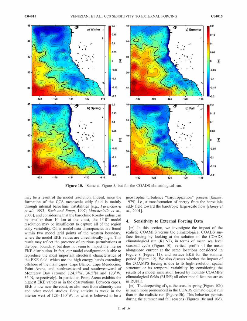
[22] In this section, we investigate the impact of therealistic COAMPS versus the climatological COADS sur-face forcing by looking at the solution of the COADSclimatological run (RUN2), in terms of mean sea levelseasonal cycle (Figure 10), vertical profile of the meanalongshore current at the same locations considered inFigure 8 (Figure 11), and surface EKE for the summerperiod (Figure 12). We also discuss whether the impact ofthe COAMPS forcing is due to its high-resolution spatialstructure or its temporal variability by considering theresults of a model simulation forced by monthly COAMPSclimatological fields (RUN5; all other model features are asin RUN1).[23] The deepening of h at the coast in spring (Figure 10b)

is much more pronounced in the COADS climatological runthan in the realistic run (Figure 5b). This behavior persistsduring the summer and fall seasons (Figures 10c and 10d),

Figure 10. Same as Figure 5, but for the COADS climatological run.


11 of 16

C04015

with a marked decrease in the meandering structure ofthe coastal jet with respect to the realistic run (Figures 5cand 5d). RUN3 (with COADS surface forcing and ECCO

BCs) presents very similar results (not shown), suggestingthat the climatological surface forcing is responsible for thereduction of the SSH meandering structure in summer and

Figure 11. Same as Figure 8, but for the COADS climatological run.


12 of 16

C04015

fall. In particular, its lower spatial resolution (compared toCOAMPS) may be a key factor in the simulation of the SSHdistribution. This is indicated by the results of RUN5 (notshown), which reveal a similar h seasonal cycle as in therealistic run.[24] The strong SSH deepening at the coast in the

COADS climatological run is consistent with a muchstronger coastal jet than that simulated in the realistic runin June (compare Figures 11b, 11d, and 11f with Figures 8b,8d, and 8f). Even more importantly, the equatorward jet isalso present at all locations in January (Figures 11a, 11c,and 11e), instead of the poleward Davidson current that isreproduced in the realistic run (Figures 8a, 8c, and 8e).RUN3 produces very similar results to the climatologicalrun, whereas RUN4 (with daily COAMPS surface forcingand Levitus BCs) as well as the run with COAMPSclimatology are able to simulate a Davidson current southof Point Sur in January (not shown). This confirms that thesurface forcing, and in particular its spatial distribution, ismainly responsible for the differences between the COADSclimatological and realistic run in the structure and seasonalcycle of the mean upper ocean circulation. The character-istics of the California Undercurrent are less affected by thechange in surface forcing, with higher discrepancies foundat Cape Mendocino (Figures 11a and 11b), but generallysimilar vertical structures found in the realistic and clima-tological runs near Monterey Bay and Point Sur (Figures 8c,8d, 8e, 8f, 11c, 11d, 11e, and 11f).[25] The impact of the COAMPS surface forcing is also

evident in the surface EKE field (compare Figures 9b and12). In the COADS climatological run, the EKE levels eastof �126W are on average almost half as much as those inthe realistic run. Moreover, the EKE spatial structure inFigure 12 less faithfully reproduces that observed fromin situ drifters (Figure 9b), exhibiting less developed bandsnear Cape Mendocino and Point Arena, no energy offshoreof Cape Blanco, and only one energetic band extendingoffshore of Point Reyes and Monterey Bay. These resultsare in agreement with the reduced meandering structure of

the mean sea level field (Figure 10), suggesting that theclimatological surface forcing in our simulation inhibitsthe development of a convoluted equatorward jet duringthe summer and fall seasons, and in the end produces a lessenergetic coastal California circulation. Inspection of thesummer EKE from RUN5 (not shown) reveals a similarspatial structure as in the realistic run, but generally lowervalues of EKE. This indicates that the temporal variabilityof the atmospheric forcing, as well as its spatial distribution,contribute to the overall energy structure of the CCS.

5. Discussion

[26] In this paper, we perform a high-resolution ROMSsimulation of the CCS, with an emphasis on the circulationof the northern and central California region, using arealistic model data product as external forcing for boththe ocean surface (COAMPS) and the lateral open bound-aries (ECCO-GODAE). By comparing the model resultswith available observations and previous modeling efforts,we find that the present model solution well represents themean features and seasonal cycle of the California coastalcirculation. We also perform a sensitivity analysis to spe-cifically study the effect of realistic versus climatologicalforcing on the large-scale and mesoscale dynamics of theCCS.[27] We concentrate on this type of forcing comparison,

time-dependent, high-resolution forcing versus climatology,mainly because previous regional model investigations ofthe CCS [e.g., Marchesiello et al., 2003; Batteen et al.,2003; Batteen, 1997] adopt climatological forcing for boththe surface and lateral boundary conditions. Our focus hereis on the impact that realistic atmospheric forcing has on theannual cycle of the CCS. Studies of interannual variabilitywould obviously also require the use of time-dependentrealistic surface forcing. This is, for instance, addressed byCurchitser et al. [2005], who carried out multiscale modelsimulations of the North Pacific, downscaling from a basin-wide, climatologically forced setup to a regional, realisti-cally forced configuration, with the objective of studyingthe effects of interannual and climate processes on thephysical and ecosystem dynamics of the northeast Pacific.Another atmospheric product commonly used to driveoceanic models is the NCEP/NCAR reanalysis product,which has the advantage of covering a long period of timebetween the 1950s to the present, but is characterized by alower horizontal resolution (�2.5�) than that of COADS.Our own experience using NCEP/NCAR for the presenthigh-resolution CCS study indicate that the resulting circu-lation is not as well reproduced as when using the clima-tological forcing. In particular, the mesoscale eddy energy isvery weak south of Cape Blanco and the energetic bands offthe main promontories are almost absent.[28] While the use of a realistic, high-resolution forcing

data product such as COAMPS versus the use of a clima-tological forcing is generally not considered fundamentalfor reproducing the mesoscale internal variability of anoceanic system, this is possibly not true for a complexsystem like the CCS. It is reasonable to think, for example,that a highly resolved spatial wind structure in a coastalupwelling region (COAMPS resolution is 3–9 km along theCalifornia coast while COADS resolution is 1� everywhere)

Figure 12. Same as Figure 9a, but for the COADSclimatological run.


13 of 16

C04015

leads to a better representation of the upper ocean stratifi-cation and associated cross-shore and alongshore circulationstructure. Furthermore, a high-resolution wind field is ableto reproduce the locally intensified wind stress curl thatoccurs within 50–100 km from the coast, and which is nowrecognized to contribute substantially to coastal upwellingthrough the Ekman pumping mechanism [Enriquez andFriehe, 1995; Pickett and Paduan, 2003; Koracin et al.,2004]. Di Lorenzo [2003] also finds that spatially wellresolved wind stress and wind stress curl are fundamentalin reproducing the seasonal cycle of the mean SouthernCalifornia Bight circulation and the SCB coastal polewardflow in late summer and fall. Finally, numerical studies byCastelao and Barth [2006] show that both the presence ofan irregular coastline geometry (capes) and phenomena ofwind intensification in proximity of the coastal promonto-ries are responsible for the separation of an upwelling jetfrom the coast. Such results suggest that a spatially wellresolved wind field would enhance the coastal jet separationat the main capes located along the U.S. West Coast southof Cape Blanco, likely intensifying the jet turbulent behav-ior and consequent eddy activity downstream of theselocations.[29] An important contribution of this paper is indeed to

confirm that realistic surface forcing such as COAMPS, andin particular their high-resolution spatial structure, greatly

improve not only the simulation of the CCS mean circula-tion but also of its mesoscale eddy activity. The seasonalcycle of the upper ocean coastal alongshore jet is betterrepresented, as well as its spatial structure. Moreover, themesoscale eddy field associated with the jet instabilities ismore intense and displays a more realistic spatial distribu-tion than that in the COADS climatological run. The nextstep of this investigation will be to increase the horizontalresolution of the ROMS model, in order to better resolve thebaroclinic Rossby radius of deformation and provide aneven more realistic representation of the coastal jet insta-bility processes.[30] Although not discussed within this text, we investi-

gate the impact of using different lateral boundary forcingfields on the model solution. Sensitivity studies are con-ducted to verify whether higher-temporal-resolution andhigher-spatial-resolution BC products provide an improve-ment over using 1� monthly ECCO-GODAE fields. Wetherefore perform simulations using the 1/8� monthlyECCO2 product (High-Resolution Global-Ocean and SeaIce Data Synthesis Phase II of the ECCO project available athttp://ecco2.jpl.nasa.gov/products/output/cube/), a 1� dailyECCO-GODAE product (ECCO-GODAE Iteration 216available at http://www.ecco-group.org/products.htm), andvarious choices of boundary condition schemes (clamped andradiation). The results show that, while certain improvements

a)

b)

c)

d)

e)

f )

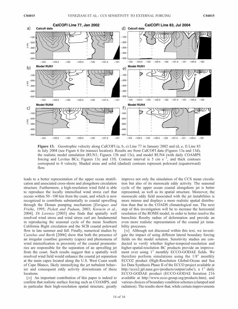
Figure 13. Geostrophic velocity along CalCOFI (a, b, c) Line 77 in January 2002 and (d, e, f) Line 83in July 2004 (see Figure 6 for transect location). Results are from CalCOFI data (Figures 13a and 13d),the realistic model simulation (RUN1; Figures 13b and 13e), and model RUN4 (with daily COAMPSforcing and Levitus BCs; Figures 13c and 13f). Contour interval is 5 cm s�1, and thick contourscorrespond to 0 velocity. Shaded areas and solid (dashed) contours represent poleward (equatorward)flow.


14 of 16

C04015

are introduced (lower boundary EKE values when usingradiation conditions, and a better representation of thegeostrophic transport across northern CalCOFI Lines whenusing ECCO2 BCs), the overall circulation is not as wellrepresented as in our control RUN1. This is likely becauselarger inconsistencies exist between the ROMS interiorcirculation and the considered higher-resolution ECCO prod-ucts, which are more difficult to eliminate by the openboundary condition scheme.[31] Finally, we investigate the difference between using

realistic (ECCO-GODAE) and climatological (Levitus) lat-eral boundary forcing fields. Though we find quantitativechanges to our measures characterizing the circulation, ourresults are not conclusive as some metrics improve withrealistic boundary conditions and others with climatologicalfields. For instance, the subsurface salinity bias in theCalCOFI region is slightly improved with realistic lateralforcing, whereas the surface bias is slightly worsened.An example of geostrophic velocity derived from theCalCOFI temperature and salinity sections for RUN1 andRUN4 is presented in Figure 13, for Line 77 in January2002 (Figures 13a, 13b, and 13c) and Line 83 in July 2004(Figures 13d, 13e, and 13f). As exemplified in Figure 13,while the realistic boundary forcing produces much betterresults in some cases, a different scenario may occur atdifferent times and/or locations. Furthermore, the qualitativestructure of meridional velocity within the previously con-sidered cross-shore sections (not shown) is not substantiallyaltered when using the realistic versus the climatologicalBCs, nor is there a significant change to the EKE structure.Future studies (and additional in situ data sets available formodel evaluation) may further identify the impact of thespecific choice of lateral boundary forcing, particularly onsubsurface features, but our initial investigation indicatesthat surface forcing plays a more dominant role on chosenCCS metrics than do lateral boundary fields. This outcomeleads naturally to part 2, where we quantitatively investigatethe sensitivities of the California coastal circulation to large-scale external forcing mechanisms and to internal dynamicsby adopting an adjoint model approach.

[32] Acknowledgments. The authors wish to thank Patrick Heimbachfor his helpful comments on the paper and Gregoire Broquet and EnriqueCurchitser for useful scientific discussions. The ECCO-GODAE data wasprovided by the ECCOConsortium for Estimating the Circulation and Climateof the Ocean funded by the National Oceanographic Partnership Program(NOPP). This research was funded by NOPP project NA05NOS4731242.

ReferencesAmante, C., and B. W. Eakins (2001), 2-Minute Gridded Global Relief Data(ETOPO2), http://www.ngdc.noaa.gov/mgg/global/, Natl. Geophys. DataCent., Boulder, Colo.

Barth, J. A., S. D. Pierce, and R. L. Smith (2000), A separating coastalupwelling jet at Cape Blanco, Oregon and its connection to the CaliforniaCurrent System, Deep Sea Res., Part II, 47, 783–810.

Batteen, M. L. (1997), Wind-forced modeling studies of currents, mean-ders, and eddies in the California Current System, J. Geophys. Res., 102,985–1010.

Batteen, M. L., N. J. Cipriano, and J. T. Monroe (2003), A large-scaleseasonal modeling study of the California Current System, J. Oceanogr.,59, 545–562.

Capet, X. J., P. Marchesiello, and J. C. McWilliams (2004), Upwellingresponse to coastal wind profiles, Geophys. Res. Lett., 31, L13311,doi:10.1029/2004GL020123.

Castelao, R. M., and J. A. Barth (2006), The relative importance of windstrength and along-shelf bathymetric variations on the separation of acoastal upwelling jet, J. Phys. Oceanogr., 36, 412–425.

Centurioni, D. C., J. C. Ohlmann, and P. P. Niiler (2008), Permanentmeanders in the California Current System, J. Phys. Oceanogr., 38,1690–1710.

Cervantes, B. T. K., and J. S. Allen (2006), Numerical model simulations ofcontinental shelf flows off northern California, Deep Sea Res., Part II, 53,2956–2984.

Chapman, D. C. (1985), Numerical treatment of cross-shelf open bound-aries in a barotropic coastal ocean model, J. Phys. Oceanogr., 15,1060–1075.

Chereskin, T. K., M. Y. Morris, P. P. Niiler, P. M. Kosro, R. L. Smith, S. R.Ramp, C. A. Collins, and D. L. Musgrave (2000), Spatial and temporalcharacteristics of the mesoscale circulation of the California Current fromeddy-resolving moored and shipboard measurements, J. Geophys. Res.,105, 1245–1269.

Collins, C. A., N. Garfield, T. A. Rago, F. W. Rischmiller, and E. Carter(2000), Mean structure of the inshore countercurrent and California under-current off Point Sur, California, Deep Sea Res., Part II, 47, 765–782.

Conkright, M., S. Levitus, T. O’Brien, T. Boyer, J. Antonov, and C. Stephens(1998), World Ocean Atlas 1998, CD-ROM Data Set Documentation,Tech. Rep. 15, Natl. Oceanogr. Data Cent., Silver Spring, Md.

Conkright, M., R. A. Locarnini, H. E. Garcia, T. D. O’Brien, T. P. Boyer,C. Stephens, and J. I. Antonov (2002), World Ocean Atlas 2001: ObjectiveAnalyses, Data Statistics, and Figures, CD-ROM Documentation, Tech.Rep. 17, Natl. Oceanogr. Data Cent., Silver Spring, Md.

Curchitser, E. N., D. B. Haidvogel, A. J. Hermann, E. L. Dobbins, T. M.Powell, and A. Kaplan (2005), Multi-scale modeling of the North PacificOcean: Assessment and analysis of simulated basin-scale variability (1996–2003), J. Geophys. Res., 110, C11021, doi:10.1029/2005JC002902.

Davis, R. E. (1991), Observing the general circulation with floats, DeepSea Res., Part A, 38, 531–571.

Davis, R. E., and P. S. Bogden (1989), Variability on the California shelfforced by local and remote winds during the Coastal Ocean DynamicsExperiment, J. Geophys. Res., 94, 4763–4783.

Di Lorenzo, E. (2003), Seasonal dynamics of the surface circulation inthe Southern California Current System, Deep Sea Res., Part II, 50,2371–2388.

Doglioli, A. M., M. Veneziani, B. Blanke, S. Speich, and A. Griffa (2006), ALagrangian analysis of the Indian-Atlantic interocean exchange in a regio-nal model, Geophys. Res. Lett., 33, L14611, doi:10.1029/2006GL026498.

Doyle, J. D. (1997), The influence of mesoscale orography on a coastal jetand rainband, Mon. Weather Rev., 125, 1465–1488.

Doyle, J. D., Q. Jiang, Y. Chao, and J. Farrara (2008), High-resolutionatmospheric modeling over the Monterey Bay during AOSN II, DeepSea Res., Part II, in press.

Ebert, E. E., U. Damrath, W. Wergen, and M. E. Baldwin (2003), TheWGNE assessment of short-term quantitative precipitation forecasts,Bull. Am. Meteorol. Soc., 84, 481–492.

Enriquez, A. G., and C. A. Friehe (1995), Effects of wind stress and windstress effects of wind stress and wind stress curl variability on coastalupwelling, J. Phys. Oceanogr., 25, 1651–1671.

Fairall, C. W., E. F. Bradley, J. S. Godfrey, G. A. Wick, J. B. Edson, andG. S. Young (1996a), Cool-skin and warm-layer effects on sea surfacetemperature, J. Geophys. Res., 101, 1295–1308.

Fairall, C. W., E. F. Bradley, D. P. Rogers, J. B. Edson, and G. S. Young(1996b), Bulk parameterization of air-sea fluxes for tropical ocean globalatmosphere Coupled-Ocean Atmosphere Response Experiment, J. Geo-phys. Res., 101, 3747–3764.

Flather, R. A. (1976), A tidal model of the north-west European continentalshelf, Mem. Soc. R. Sci. Liege, 6(10), 141–164.

Fratantoni, D. M. (2001), North Atlantic surface circulation during the1990s observed with satellite-tracked drifters, J. Geophys. Res., 106,22,067–22,093.

Freeland, H., P. Rhines, and H. T. Rossby (1975), Statistical observations ofthe trajectories of neutrally buoyant floats in the North Atlantic, J. Mar.Res., 33, 383–404.

Gan, H. P., and J. S. Allen (2002a), A modeling study of shelf circulationoff northern California in the region of the Coastal Ocean DynamicsExperiment: Response to relaxation of upwelling winds, J. Geophys.Res., 107(C9), 3123, doi:10.1029/2000JC000768.

Gan, H. P., and J. S. Allen (2002b), A modeling study of shelf circulationoff northern California in the region of the Coastal Ocean DynamicsExperiment 2. Simulations and comparisons with observations, J. Geo-phys. Res., 107(C11), 3184, doi:10.1029/2001JC001190.

Gruber, N., H. Frenzel, S. C. Doney, P. Marchesiello, J. C. McWilliams,J. R. Moisan, J. J. Oram, G. K. Plattner, and K. D. Stolzenbach (2006),Eddy-resolving simulation of plankton ecosystem dynamics in the Cali-fornia Current System, Deep Sea Res., Part I, 53, 1483–1516.

Haidvogel, D. B., H. G. Arango, K. Hedstrom, A. Beckmann, P. Malanotte-Rizzoli, and A. F. Shchepetkin (2000), Model evaluation experiments in


15 of 16

C04015

the North Atlantic basin: Simulations in nonlinear terrain-followingcoordinates, Dyn. Atmos. Oceans, 32, 239–281.

Haney, R. L. (1991), On the pressure force over steep topography in sigmacoordinate ocean models, J. Phys. Oceanogr., 21, 610–619.

Haney, R. L., R. A. Hale, and D. E. Dietrich (2001), Offshore propagationof eddy kinetic energy in the California Current, J. Geophys. Res., 106,11,709–11,718.

Hickey, B. M. (1979), The California Current System: Hypotheses andfacts, Prog. Oceanogr., 8, 191–279.

Hickey, B. M. (1998), Coastal oceanography of western North Americafrom the tip of Baja California to Vancouver Island, in The Sea, vol. 11,edited by A. R. Robinson and K. H. Brink, pp. 345–393, John Wiley,New York.

Hickey, B. M., E. L. Dobbins, and J. S. Allen (2003), Local and remoteforcing of currents and temperature in the central Southern CaliforniaBight, J. Geophys. Res., 108(C3), 3081, doi:10.1029/2000JC000313.

Hickey, B. M., A. MacFayden, W. Cochlan, R. Kudela, K. Bruland, andC. Trick (2006), Evolution of chemical, biological, and physical waterproperties in the northern California Current in 2005: Remote or local windforcing?, Geophys. Res. Lett., 33, L22S02, doi:10.1029/2006GL026782.

Hodur, R. M. (1997), The Naval Research Laboratory’s Coupled Ocean/Atmosphere Mesoscale Prediction System (COAMPS), Mon. WeatherRev., 135, 1414–1430.

Hodur, R. M., J. Pullen, J. Cummings, X. Hong, J. D. Doyle, P. Martin, andM. A. Rennick (2002), The Coupled Ocean/Atmosphere MesoscalePrediction System (COAMPS), Oceanography, 15, 88–98.

Koracin, D., C. E. Dorman, and E. P. Dever (2004), Coastal perturbations ofmarine-layer winds, wind stress, and wind stress curl along Californiaand Baja California in June 1999, J. Phys. Oceanogr., 34, 1152–1173.

Lagerloef, G. S. (1992), The Point Arena eddy: A recurring summer antic-yclone in the California Current, J. Geophys. Res., 97, 12,557–12,568.

Liu, W. T., K. B. Katsaros, and J. A. Businger (1979), Bulk parameteriza-tion of the air-sea exchange of heat and water vapor including the mole-cular constraints at the interface, J. Atmos. Sci., 36, 1722–1735.

Lynn, R. J., S. J. Bograd, T. K. Chereskin, and A. Huyer (2003), Seasonalrenewal of the California Current: The spring seasonal renewal of theCalifornia Current: The spring transition off California, J. Geophys. Res.,108(C8), 3279, doi:10.1029/2003JC001787.

Marchesiello, P., J. C. McWilliams, and A. F. Shchepetkin (2003), Equilib-rium structure and dynamics of the California Current System, J. Phys.Oceanogr., 33, 753–783.

Marshall, J. C., A. Adcroft, C. Hill, L. Perelman, and C. Heisey (1997a), Afinite-volume, incompressible Navier Stokes model for studies of theocean on parallel computers, J. Geophys. Res., 102, 5753–5766.

Marshall, J. C., C. Hill, L. Perelman, and A. Adcroft (1997b), Hydrostatic,quasi-hydrostatic, and nonhydrostatic ocean modeling, J. Geophys. Res.,102, 5733–5752.

McCreary, J. P. J., P. K. Kundu, and S.-Y. Chao (1987), On the dynamics ofthe California Current system, J. Mar. Res., 45, 1–32.

Moore, A. M., H. G. Arango, E. Di Lorenzo, B. D. Cornuelle, A. J. Miller,and D. J. Neilson (2004), A comprehensive ocean prediction and analysissystem based on the tangent linear and adjoint of a regional ocean model,Ocean Modell., 7, 227–258.

Noble, M. A., and S. R. Ramp (2000), Subtidal currents over the centralCalifornia slope: Evidence for onshore veering of the undercurrent and fordirect, wind-driven slope currents, Deep Sea Res., Part II, 47, 871–906.

Pares-Sierra, A., W. B. White, and C.-K. Tai (1993), Wind-driven coastalgeneration of annual mesoscale eddy activity in the California Current,J. Phys. Oceanogr., 23, 1110–1121.

Pickett, M. H., and J. D. Paduan (2003), Ekman transport and pumping inthe California Current based on the U.S. Navy’s high-resolution atmo-spheric model (COAMPS), J. Geophys. Res., 108(C10), 3327,doi:10.1029/2003JC001902.

Pierce, S. D., R. L. Smith, P. M. Kosro, J. A. Barth, and C. D. Wilson (2000),Continuity of the poleward undercurrent along the eastern boundary of themid-latitude north Pacific, Deep Sea Res., Part II, 47, 811–829.

Powell, B. S., H. G. Arango, A. M. Moore, E. Di Lorenzo, R. F. Milliff, andD. Foley (2008), 4DVAR Data Assimilation in the Intra-Americas Sea

with the Regional Ocean Modeling System (ROMS), Ocean Modell., 23,130–145.

Ramp, S. R., L. K. Rosenfeld, T. D. Tisch, and M. R. Hicks (1997), Mooredobservations of the current and temperature structure over the continentalslope off northern California 1. A basic description of the variability,J. Geophys. Res., 102, 22,877–22,902.

Rhines, P. B. (1979), Geostrophic turbulence, Annu. Rev. Fluid Mech., 11,401–441.

Rosenfeld, L. K., F. B. Schwing, N. Garfield, and D. E. Tracy (1994),Bifurcated flow from an upwelling center: A cold water source for Mon-terey Bay, Cont. Shelf Res., 14, 931–964.

Shchepetkin, A. F., and J. C. McWilliams (2005), The regional oceanicmodeling system (ROMS): A split-explicit, free-surface, topography-following-coordinate oceanic model, Ocean Modell., 9, 347–404.

Shulman, I., C. R. Wu, J. K. Lewis, J. D. Paduan, L. K. Rosenfeld, J. C.Kindle, S. R. Ramp, and C. A. Collins (2002), High resolution modelingand data assimilation in the Monterey Bay area, Cont. Shelf Res., 22,1129–1151.

Shulman, I., et al. (2007), Modeling of upwelling/relaxation events with theNavy Coastal Ocean Model, J. Geophys. Res., 112, C06023, doi:10.1029/2006JC003946.

Song, Y. T., and D. B. Haidvogel (1994), A semi-implicit ocean circulationmodel using a generalized topography-following coordinate system,J. Comput. Phys., 115, 228–244.

Strub, P. T., and C. James (2000), Altimeter-derived variability of surfacevelocities in the California Current System: 2. Seasonal circulation andeddy statistics, Deep Sea Res., Part II, 47, 831–870.

Swenson, M. S., and P. P. Niiler (1996), Statistical analysis of the surfacecirculation of the California Current, J. Geophys. Res., 101, 22,631–22,645.

Tisch, T. D., and S. R. Ramp (1997), Moored observations of the currentand temperature structure over the continental slope off northern Cali-fornia 2. The energetics of the flow off Point Sur, J. Geophys. Res.,102, 13,023–13,042.

Umlauf, L., and H. Burchard (2003), A generic length-scale equation forgeophysical turbulence models, J. Mar. Res., 61, 235–265.

Veneziani, M., A. Griffa, A. M. Reynolds, and A. J. Mariano (2004), Ocea-nic turbulence and stochastic models from subsurface Lagrangian data forthe Northwest Atlantic Ocean, J. Phys. Oceanogr., 34, 1884–1906.

Veneziani,M., C. A. Edwards, and A.M.Moore (2009), A Central Californiacoastal ocean modeling study: 2. Adjoint sensitivities to local and remotedriving mechanisms, J. Geophys. Res., doi:10.1029/2008JC004775,in press.

Wang, X., and Y. Chao (2004), Simulated sea surface salinity variability inthe tropical Pacific, Geophys. Res. Lett., 31, L02302, doi:10.1029/2003GL018146.

Warner, J. C., C. R. Sherwood, H. G. Arango, and R. P. Signell (2005),Performance of four turbulence closure models implemented using ageneric length scale method, Ocean Modell., 8, 81–113.

Werner, F. E., and B. M. Hickey (1983), The role of longshore pressuregradient in Pacific-Northwest coastal dynamics, J. Phys. Oceanogr., 13,395–410.

Wilkin, J. L., and W. F. G. Zhang (2007), Modes of mesoscale sea surfaceheight and temperature variability in the East Australian Current, J. Geo-phys. Res., 112, C01013, doi:10.1029/2006JC003590.

Wunsch, C., and P. Heimbach (2007), Practical global ocean state estima-tion, Physica D, 230(1–2), 197–208, doi:10.1016/j.physd.2006.09.040.

Wunsch, C., R. M. Ponte, and P. Heimbach (2007), Decadal trends in sealevel patterns: 1993–2004, J. Clim., 20, 5889–5911.

��J. D. Doyle, Naval Research Laboratory, 7 Grace Hopper Avenue,

Monterey, CA 93943, USA.C. A. Edwards and M. Veneziani, Ocean Sciences Department,

University of California, Santa Cruz, CA 95064, USA. ([email protected])D. Foley, Environmental Research Division, NOAA Southwest Fisheries

Science Center, 1352 Lighthouse Avenue, Pacific Grove, CA 93950, USA.


16 of 16

C04015

a central california coastal ocean modeling study: 1...

Documents