a building cycle model for an imperfect world

A Building Cycle Model for an Imperfect World

RICHARD BARRASProperty Market Analysis and University of Reading, London, UK

Received 1 August 2005Revised 26 September 2005Accepted 11 October 2005

Summary

A model of the building cycle is presented, expressed in terms of endogenous fluctuations in

development activity, vacancy and rents around an equilibrium growth path. The dynamic behaviour

of the model is determined by lags in three adjustment processes: the occupier response to changes in

rents, the development response to demand changes mediated through a rent adjustment process, and

the construction delay between starts and completions. The frequency and severity of the cycle depend

upon the values of five key parameters including the construction lag and the transmission coefficient

linking vacancy to development starts. The model has been fitted to data for the City of London office

market, yielding estimates for key parameters that are consistent with its observed cyclical

behaviour.

Keywords: Building cycles, office markets, rent adjustment, City of London

1. Property Cycles: a Return to the City of London

The Central London office markets have reached the trough of their fourth majormarket cycle of the post-war period. The current cycle, like that of the late 1980s/early1990s, has been a global phenomenon, and across Europe a synchronized cycle of officetake up, vacancy, rental growth and building has affected most markets with varyingdegrees of severity. It is, therefore, a good time to take stock of our understanding ofhow these cycles are generated, and where theory needs to be improved in the light ofrecent experience (for previous work on this topic see Barras, 1983; Barras andFerguson, 1987; Barras, 1994).

After each property boom and bust, the same two questions are always asked, ‘whydid it go wrong?’ and ‘how can we avoid it happening again?’ The answers are alsobroadly the same each time – it went wrong because of inaccurate data, incorrectforecasts and inadequate analysis by developers and investors; the solution is to improveall of these for next time. Following the global boom–bust cycle of the late 1980s/early1990s, there has been a huge investment of resources into property data-gathering,forecasting techniques and investment analysis. This has taken place against a

Author to whom correspondence should be addressed: Richard Barras, Property Market Analysis and

University of Reading, Berkshire House, 168–173 High Holborn, London WC1V 7AA, UK.

Journal of Property Research, June–September 2005, 22(2–3) 63–96

Journal of Property Research

ISSN 0959–9916 print/ISSN 1466–4453 online # 2005 Taylor & Francis

http://www.tandf.co.uk/journals

DOI: 10.1080/09599910500453905

background of economic theory increasingly dominated by the new orthodoxy of‘rational expectations’. In its most extreme form, this puts the blame for property cycleson market agents forming ‘myopic’ expectations about future prices, typically assumingthat the future will be like the present or the past. The argument goes on to say that ifagents exercise perfect foresight, cyclical fluctuations cannot be generated endogenously;rather they can only be the product of repeated exogenous shocks, the outcomes ofwhich can be predicted even if their timing cannot. This then tends to shift attention tothe search for external scapegoats, whether ill judged government intervention or acts ofGod.

However, what does perfect foresight mean in the property market? As summarizedby Wheaton (1999, p. 215) it means that developers and investors ‘perfectly understandthe equations that govern market behaviour and can thus make correct forecasts ofrents’. To someone like the author, who has spent his whole professional life repeatingthe mantra that in an imperfect world ‘all forecasts are wrong’, this is indeed startling.Let us briefly consider some of the characteristics of commercial property markets thatmake perfect foresight especially improbable:

N Since each property is unique in terms of specification and location, future rentdetermination in this heterogeneous market depends not only on future aggregatemarket conditions, but also on the precise mix of properties being transacted.

N Long leases severely constrain the elasticity of demand for property with respect tochanges in rent, so that future rent determination is strongly affected by the historicalmarket conditions embedded in unexpired leases and pre-let contracts.

N With the majority of property development being undertaken speculatively,developers can only base their predictions of future demand on measurable butindirect indicators of demand such as vacancy and take-up, much of which consists ofturnover within the existing stock.

N The construction lags between the start and completion of commercial buildings areamong the longest production delays in the capital goods sector, demanding thatproperty developers and investors be particularly far-sighted.

N So long are these construction lags that there is a significant probability of anunanticipated exogenous shock to the market occurring within the constructionperiod, confounding the most rational of expectations formed at the outset ofdevelopment.

There is no better exemplar of this imperfect world than the City of London officemarket; the largest, most liquid, best documented and most intensively measured officemarket in Europe. Consistent data series are available to provide a coherent markethistory back to 1970 and some series stretch back well into the 1960s. One par-ticularly valuable dataset is the ICHP rent index, initiated under the direction ofRussell Schiller. For the City of London, this index shows that three major cyclesin real rents peaked in 1973–74, 1988–89 and 2001, and that successive peaks andtroughs have tended to reach progressively lower levels in each cycle. The seculardownward trend in real office rents in the City over the past 40 years is indicative of animperfect market prone to endemic over-supply under the impact of successive buildingcycles.

To understand better how these cycles operate, let us now illustrate the market cyclein the City of London in terms of directly measured data series for take up, vacancy, real

64 R. Barras

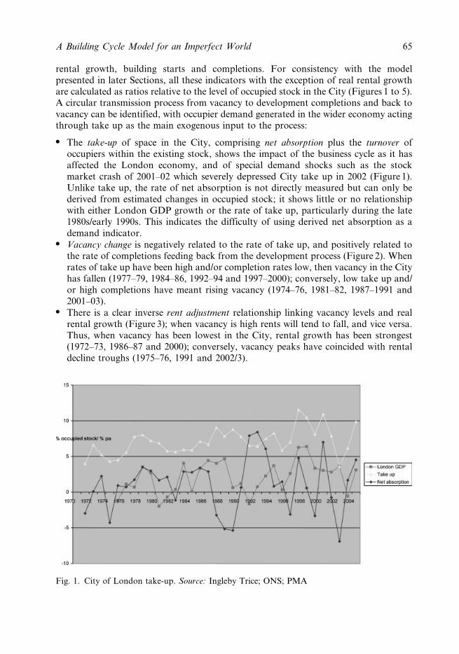
rental growth, building starts and completions. For consistency with the modelpresented in later Sections, all these indicators with the exception of real rental growthare calculated as ratios relative to the level of occupied stock in the City (Figures 1 to 5).A circular transmission process from vacancy to development completions and back tovacancy can be identified, with occupier demand generated in the wider economy actingthrough take up as the main exogenous input to the process:

N The take-up of space in the City, comprising net absorption plus the turnover ofoccupiers within the existing stock, shows the impact of the business cycle as it hasaffected the London economy, and of special demand shocks such as the stockmarket crash of 2001–02 which severely depressed City take up in 2002 (Figure 1).Unlike take up, the rate of net absorption is not directly measured but can only bederived from estimated changes in occupied stock; it shows little or no relationshipwith either London GDP growth or the rate of take up, particularly during the late1980s/early 1990s. This indicates the difficulty of using derived net absorption as ademand indicator.

N Vacancy change is negatively related to the rate of take up, and positively related tothe rate of completions feeding back from the development process (Figure 2). Whenrates of take up have been high and/or completion rates low, then vacancy in the Cityhas fallen (1977–79, 1984–86, 1992–94 and 1997–2000); conversely, low take up and/or high completions have meant rising vacancy (1974–76, 1981–82, 1987–1991 and2001–03).

N There is a clear inverse rent adjustment relationship linking vacancy levels and realrental growth (Figure 3); when vacancy is high rents will tend to fall, and vice versa.Thus, when vacancy has been lowest in the City, rental growth has been strongest(1972–73, 1986–87 and 2000); conversely, vacancy peaks have coincided with rentaldecline troughs (1975–76, 1991 and 2002/3).

Fig. 1. City of London take-up. Source: Ingleby Trice; ONS; PMA

A Building Cycle Model for an Imperfect World 65

N A development supply relationship can be seen to link rental change to the rateof building starts (Figure 4), the higher the rate of rental growth, the more theprofitability of development is increasing and therefore the higher the rate of startsinitiated by developers. Thus peak periods of real rental growth in the City (1972,1987 and 2000) have generated a subsequent peak in development starts, typicallywith a one year lag (1973, 1988 and 2001). There is some evidence here ofdevelopment expectations anticipating future rent levels, insofar as current rentalgrowth is an indicator of future rent levels.

Fig. 2 .City of London vacancy change. Source: City Corporation; EGiLOD; PMA

Fig. 3. City of London rent adjustment. Source: ICHP; CBRE; Ingleby Trice; DoE; PMA

66 R. Barras

N Owing to the scale of the building projects being undertaken, there is a substantialconstruction delay between starts and completions (Figure 5). Peaks of starts in theCity (1973, 1988 and 2001) have been followed by peaks in completions two to threeyears later (1976, 1991 and 2003).

The mathematical model presented below incorporates each of these stages of thetransmission process by which the building cycle, and related market cycles in vacancy

Fig. 4. City of London development reaction. Source: ICHP; CBRE; City Corporation:EGiLOD; PMA

Fig. 5. City of London building cycle. Source: City Corporation; EGiLOD; PMA


and rents, are propagated. First, we shall briefly review the theoretical background tothe model.

2. Modelling Property Cycles

Property cycles can usefully be visualized as fluctuations in market variables generatedaround an equilibrium growth path for an economy in which the occupier demand forproperty is met by a development sector engaged in building construction and aninvestment sector engaged in building ownership. For such an economy, a basictheoretical steady state growth path can be characterized by the following ‘stylized facts’(Kaldor, 1961, p. 178 ):

N a rate of output growth given by the sum of the rate of technical progress, or labourproductivity, and the rate of labour force growth;

N a capital stock, including building stock, growing at the same rate as economicoutput, allowing for a constant rate of slack capacity, including building vacancy,and a constant rate of depreciation;

N capital per worker, including building capital per worker, rising at the rate of labourproductivity growth;

N a constant capital output ratio, implying that building capital per unit of outputremains constant;

N real wages rising in line with labour productivity, and all other real prices, includingproperty rents and capital values, remaining constant;

N a constant rate of profit, including development profit, so that the shares of capitaland labour in total income remain constant.

This growth model has been used to analyze the long-run contribution of buildinginvestment to the growth of the UK economy since the mid nineteenth century, showinghow the steady state growth path is modified where there is continuous substitutionaway from buildings towards equipment capital, because the latter embodies a higherrate of technical progress (Barras, 2001).

The aim of this paper is to describe how building cycles are generated and sustainedaround such a growth path, working towards a synthesis of cycle and growth theory ofthe type pioneered by Goodwin (1967). For this purpose, it is helpful to convertextensive market variables such as occupancy, net absorption, take up, vacancy,building starts and completions into ratios with respect to one growth variable, chosenhere to be occupied stock, so that their magnitudes are not growth dependent andcyclical fluctuations can more readily be isolated. With this approach market quantitiessuch as vacancy and building starts, together with price variables such as rent andcapital value, can be expressed as fluctuating relative to their ‘natural value’ defined bythe equilibrium growth path.

Business cycle theory offers two approaches to explaining fluctuations around agrowth trajectory of the type outlined above. As already indicated, one emphasizes therole of repeated exogenous shocks or disturbances as the generators of cyclicalbehaviour, and the other focuses on the processes by which an initial displacement awayfrom the equilibrium growth path can trigger self-sustaining endogenous cycles (Dore,

68 R. Barras

1993). The latter approach is adopted in this study. Endogenous cycle theory shows thatit is the speed and strength of the adjustment response of an economic system to aninitial displacement that is a crucial determinant of its subsequent dynamic behaviour.The slower the speed of adjustment, the more likely it is that persistent cyclical fluc-tuations will be generated, and theory shows that two adjustment lags is the minimumnecessary to generate an endogenous cycle.

The multiplier-accelerator model (Samuelson, 1939) is the classic demonstration ofthis necessary condition; lags on the multiplier relationship between output andconsumption, and on the accelerator relationship between consumption and investmentcan be shown to generate cyclical fluctuations in output under certain conditionsattached to the model parameters. An alternative approach was developed by Kalecki(1937), who was the first to focus explicitly upon lags in the production of capital goodsas a driver of business cycles; from time to time economists have returned to this idea,most notably Kydland and Prescott (1982) with their equilibrium growth modelincorporating the multi-period construction of capital goods.

To highlight where cycle-inducing adjustment lags have been identified in theproperty market, we can examine the literature on multi-equation models of marketstructure (see Ball et al., 1998; McDonald, 2002), making use of the separate stages ofthe transmission process identified in Section 1.

Take-up and Net Absorption

Most property market models incorporate a demand equation in which desired buildingstock is expressed as a direct function of economic activity and an inverse function of thereal rent level, acting to vary the occupancy rate around its natural level (thoughestimation often shows this rent effect to be weak, because of the inelasticities of propertydemand due to long leases and high moving costs). Desired stock may then be translatedinto actual net absorption by means of a partial stock adjustment process, in effectoperating over several periods (Wheaton, 1987; Hendershott et al., 1999). An explicittake up equation combining net absorption and turnover is not usually specified.

Vacancy Change

A crucial element of real estate markets, curiously ignored in some recent models, is thelandlord demand to hold vacant space as a buffer stock to accommodate tenant turnover,allow for demand uncertainty and provide the option to delay lettings in expectation ofbetter future market conditions. (McDonald, 2000) argues that this demand for vacantspace tends to vary negatively with the real rent level, acting as its opportunity cost, andthat there is a natural vacancy rate co-determined with the natural level of real rentsalong the equilibrium growth path. Most studies assume a constant natural rate aroundwhich vacancy adjusts positively to the addition of development completions andnegatively to net absorption, though Sivitanides (1997) explores how market conditionsmay vary the natural rate through time. It can be assumed that vacancy adjustments arelagged. For example, Grenadier(1995) uses the analogy of a financial option to explainhow there can be stickiness in vacancy in the face of changing occupier demand, asowners hold buildings empty in anticipation of higher future rents in a rising market, orconversely offer incentives for occupiers to stay on in a falling market.


Rent Adjustment

There is a long tradition of real estate models incorporating a rent adjustment equation,drawing upon macroeconomic models relating wage or price inflation to deviations inunemployment from its natural rate. At its simplest, the adjustment equation expressesreal rental change as a function of the gap between the natural vacancy rate and thelagged actual rate. The more partial the relationship, the stickier are rents in response toa change in vacancy (see Smith, 1974 for an early application to the rental housingmarket; Rosen, 1984; and Wheaton, 1987, for subsequent applications to the officemarket). The view has developed that this partial adjustment formulation is theoreticallyinadequate, because the natural or equilibrium rent level is unspecified which meansthat, for example, supply shocks can force real rents to progressively lower levels.Wheaton et al. (1997) propose a model relating rental change to the gap between thenatural rent and lagged actual rent. Hendershott (1995) prefers to express rental changeas a function of both the vacancy gap and the rent gap, the rent gap acting as astabilizing feedback mechanism that allows rents to start recovering before vacancy hasfallen to its natural rate during periods of over-supply. A separate time variant equationfor natural rent can also be included, for example expressed as a product of the buildingreplacement cost and the sum of the operating cost ratio, depreciation rate and realinterest rate, treating rent as a user cost of capital (Hendershott et al., 1999). Analternative to the rent adjustment equation is to model rental change via a reduced formsupply-demand equation, incorporating demand variables such as office employment orconsumer spending, and a supply variable such as building stock; again laggedadjustment can be introduced into this framework (see Hendershott et al., 2002).

Development Supply

The development equation that has most commonly been adopted expresses the level ofdevelopment activity (starts or completions) as a function of development profitability,which is broken down into its components of capital value less construction costs, landcosts and capital costs (for one of the most complete versions, see Key et al., 1994). Withdata on property and land prices difficult to obtain, and estimation often showingconstruction costs and capital costs to be insignificant, the standard developmentequation can reduce to a supply relationship between development activity and rents(Ball et al., 1998). Because of uncertainty, the development reaction to changes inmarket conditions may be lagged, and uncertainty may explicitly be included in thedevelopment equation through the some measure of historic market volatility (Tsolacosand McGough, 1999). Few models recognize explicitly that, along with the natural rentlevel and vacancy rate, the equilibrium growth path defines a natural rate of buildingstarts, satisfying the growth and replacement components of demand, around which theactual rate of starts varies according to market conditions.

Construction Delay

Once the development decision has been made, the extensive ‘time to build’ delaybetween construction starts and completions lies at the heart of endogenous buildingcycle generation (for a counter view, see Dokko et al., 2001). As discussed in Section 1,

70 R. Barras

this delay challenges developers to formulate expectations about market conditionsseveral years ahead; various predictors of future demand growth have been proposed,such as historic employment growth (Hekman, 1985) and interest rates (Kling andMcCue, 1987). However, because the projection of future demand is so difficult,developer behaviour may be informed by no more than naı̈ve expectations or ‘habitpersistence’, whereby current conditions or past trends are extrapolated into the future(Antwi and Henneberry, 1995). One attempt to capture adaptive expectations indeveloper behaviour uses lagged first differences in rents and capital values in thedevelopment equation (Tsolacos et al., 1998). Given that separate data on starts as wellas completions is often not available, an explicit construction delay relationship may notbe incorporated into multi-equation property market models, but rather it is implied bylags in the response of completions to rents. In some cases, no construction delay isassumed at all (Wheaton et al., 1997).

In a previous building cycle model (Barras, 1983), the author combined a constructionlag with a partial stock adjustment equation, based upon the flexible accelerator model,to generate a set of second order difference equations in development starts thatexhibited cyclical behaviour within a specified range of parameter values. The stockadjustment process relates the level of building starts directly to a proportion of the gapbetween current desired stock and available stock from the previous period. This processcan most appropriately be applied in owner-occupier segments of the property market,where knowledge of future space requirements can be translated directly intodevelopment orders (see Bischoff, 1970, for an early application of the flexibleaccelerator to modelling non-residential building, and Wheaton and Torto, 1990, for theapplication of such a model to the industrial sector).

However in most parts of the property market the link between changes in occupierdemand and the speculative supply response of developers is more indirect, beingmediated through vacancy and rents, and so a new version of the model is presentedhere, with a linked rent adjustment and development supply process substituted for thedirect stock adjustment process of the previous model. On the basis of both experienceand the empirical evidence (see McDonald, 2002) the model assumes an imperfect worldof relatively inelastic occupier demand and elastic developer supply with respect to rents,as well as myopic developer expectations about rents at the time of completion. Section3 sets out the equation system, Section 4 uses an analytical solution of the basic linearmodel plus simulations of more complex versions to illustrate the conditions underwhich cyclical behaviour is generated, and Section 5 reports the results of estimating thekey model relationships using the data for the City of London office market introducedin Section 1. There are similarities to the simulation approach adopted in Wheaton(1999), and though the model structure is rather different, the results achieved arebroadly consistent. A more extensive treatment of the model, and its application toexplain the incidence and behaviour of building cycles in a variety of sectors, locationsand periods will appear in Barras (forthcoming).

3. The Model

The model is developed as a series of linear difference equations, in which the dynamicchange in market variables occurs over discrete periods. Flow variables, such as output,


take up and development starts are defined as a cumulative total during each period,while the levels of stock variables such as building capital, vacancy and rents are definedat the end of one period and the start of the next. For a general introduction todifference equations, see Elaydi, 1996; for the application of difference equation modelsin business cycle theory, see Gabisch and Lorenz, 1989.

3.1. Demand for Building Stock

Assume an economy with a level of aggregate output Yt during time period t growing ata constant rate e,

Yt~ 1zeð ÞYt�1, ð1Þ

where e5v+w is the constant rate of output growth, comprising the sum of the labourforce growth rate v and rate of technical progress w.

The quantity of occupied building stock Bt required to sustain the economy operatingat level of output Yt can be expressed as a function of a building capital-output ratio oroccupancy rate at,

Bt~atYt ð2Þ

For the basic version of the model we shall assume a constant occupancy rate that isrent inelastic, i.e. at5a*; a rent elastic version is introduced in Section 3.9.

The desired level of total building stock K*t over the period consists of the

occupied stock Bt plus an additional component of ‘natural vacancy’ V*t, required as a

buffer stock to accommodate both the expansion of occupier demand as the economygrows, and the regular turnover of occupiers moving between buildings as theirrequirements change,

K�t ~BtzV�t : ð3Þ

The required level of vacant space can be expressed in terms of a constant natural

vacancy rate v* applied to the occupied stock, sufficient to ensure the efficientfunctioning of the market,

V�t ~v�Bt, ð4Þgiving

K�t ~ 1zv�ð ÞBt ð5Þ

If output growth equation (1) is applied to equations (2) and (5), it can be seen that, aslong as the occupancy rate is constant, the occupied building stock Bt and desired totalstock K*

t also both increase by the constant rate of output growth e,

Bt~ 1zeð ÞBt�1, ð6Þ

and

72 R. Barras

K�t ~ 1zeð ÞK�t�1 ð7Þ

3.2. Occupier Take-up

During each time period t, a quantum of building stock Ut is taken up by occupiers,consisting of two components – the net absorption of occupied stock Nt, resulting fromthe additional demand created by the growth of the economy, and the turnover Tt,resulting from existing occupiers moving between buildings to satisfy their changingrequirements. Take-up is thus given by

Ut~NtzTt, ð8Þ

with its two components defined as

Nt~Bt�Bt�1, ð9Þand

Tt~tBt�1, ð10Þ

where net absorption comprises the increase in occupied space between one period andthe next, and turnover is expressed as a constant turnover rate t applied to the level ofoccupied stock at the beginning of the period.

Combining equations (8) to (10) and dividing through by Bt-1 produces anequation in the rate of take up ut5Ut/Bt-1 expressed in terms of the level of occupiedstock

ut~ Bt=Bt�1ð Þ� 1� tð Þ

Substituting from equation (2), the rate of take up becomes a function of the outputgrowth rate, the occupancy rate and the turnover rate

ut~ atYt=at�1Yt�1ð Þ� 1� tð Þ, ð11Þ

and with steady state output growth, as expressed by equation (1), plus a constantoccupancy rate at5a*, equation (11) simplifies to the sum e+t as an expression for thenatural take up rate u*.

3.3. Development starts

The required level of building investment It over time period t, is a function of twocomponents of demand for new space: induced investment In

t and replacementinvestment Ir

t,

It~Int zIr

t : ð12Þ


Induced investment is a response to the demand for additional space, expressed as thedifference between the desired level of building stock during the period K*

t and theactual stock available at the end of the previous period Kt-1,

Int ~K�t�Kt�1: ð13Þ

Replacement demand can be expressed as the product of a constant depreciation rated applied to the level of building stock inherited from the previous period,

Irt~dKt�1: ð14Þ

Combining equations (13) and (14),

It~K�t� 1� dð ÞKt�1: ð15Þ

Adapting the concept of the flexible accelerator first developed by Chenery (1952), theplanned level of building starts St during the period consists of the required level ofinvestment It adjusted by a reaction coefficient c,

St~c K�t� 1� dð ÞKt�1

� �: ð16Þ

The reaction coefficient allows for investor expectations about the future demandfor space, given the lags inherent in the building process, but also the uncertaintysurrounding those expectations. As already noted in Section 2, planned buildingstarts can be translated directly into actual building orders according to equation (16) ina completely owner-occupier economy, in which all occupiers undertake their ownbuilding investment. However, in reality, most building activity is undertaken by aseparate development sector that cannot know at first hand the investment plans ofoccupiers. Rather, developers must respond indirectly to investment demand as it ismediated through the market signals of vacancy and rents or prices.

3.4. Relative Vacancy

Assume that, at the end of the previous time period, the actual level of building stockKt21 relative to occupied stock Bt21 did not match the desired level K*

t21, i.e.Kt21?K*

t21. Adapting equation (3), this implies a similar deviation between theactual and required or natural level of vacant space at the end of t21, i.e. Vt21?V*

t21,where

Vt�1~Kt�1�Bt�1: ð17Þ

The required level of starts St over the current period can then be broken down intotwo components: a natural level of starts S*

t required to increase the stock from theprevious desired level K*

t21 to new desired level K*t, and a correction St2S*

t required tocompensate for the previous deviation in stock K*

t212Kt21. Equation (16) can beexpanded to make these two components explicit,

74 R. Barras

St~c K�t� 1� dð ÞK�t�1

� �zc 1� dð Þ K�t�1�Kt�1

� �,

where the first term equates to the natural level of starts S*t and the second is the

response to the deviation in stock at the end of t21, giving

St~S�t zc 1� dð Þ K�t�1�Kt�1

� �, ð18Þ

with

S�t ~c K�t� 1� dð ÞK�t�1

� �: ð19Þ

It has already been shown in equation (7) that, with a constant occupancy rate,desired total stock K*

t grows at the constant rate of output growth e; under theseconditions it can be seen from equation (19) that this also defines the rate of growth ofnatural starts

S�t ~ 1zeð ÞS�t�1: ð20Þ

Following equations (3) and (17), the deviation in stock K*t212Kt21 in equation (18)

can be replaced by the deviation in vacant space V*t212Vt21, so that

St�S�t ~c 1� dð Þ V�t�1�Vt�1

� �: ð21Þ

This yields an equation expressing the required level of starts relative to their naturallevel during the current period as a function of the actual level of vacancy relative to itsnatural level at the start of the period.

3.5. Natural Rate of Starts

Dividing through by the level of occupied stock Bt21 transforms equation (21) into arelationship between the relative rates of starts and vacancy such that

st�s�t ~c 1� dð Þ v��vt�1ð Þ, ð22Þ

where st5St/Bt21 is the required rate of starts expressed in terms of the level of occupiedstock at the start of the period, st

*5S*t/Bt21 is the natural rate of starts required to

maintain the natural vacancy rate given by v*5V*t21/Bt21, and vt215Vt21/Bt21 is the

actual vacancy rate at the start of the period.

Substituting equations (5) and (7) into natural starts equation (19), it can be seen thatwhen the occupancy rate is constant the natural rate of starts s* is also a constant,

s�t ~s�~c 1zv�ð Þ ezdð Þ, ð23Þ

given by the sum of the induced and replacement components of investment demand, as


represented by the output growth rate and the depreciation rate, moderated by thereaction coefficient and boosted by the natural vacancy rate.

3.6. Rent adjustment

While the observed vacancy rate vt-1 at the start of the current period provides a partialsignal to developers, it is not sufficient to enable them to judge the required rate of startswithout direct knowledge about the natural vacancy and start rates in the market. Forthis, they need the further, indirect signal provided by property rents or prices. Thefollowing analysis is expressed in terms of rents; an identical formulation can be derivedusing prices or capital values, which requires the formulation of separate equations forthe determination of property yields. Myopic pricing is assumed, in that developers areforming price expectations on the basis of current real rents at the start of construction,rather than a correct forecast of their value at completion; however current rentalchange as well as current rent level is allowed to influence developer behaviour,introducing some expectations effect by signifying improving or deteriorating marketconditions.

Assume that, in equilibrium, the market establishes a real level of natural rent r*

that on the demand side provides a cost of capital affordable enough compared withother factor costs for occupiers to utilize the total stock of space up to its naturalvacancy rate v*, and on the supply side maintains a natural rate of profit sufficientfor developers to undertake the natural rate of building starts s* when set against theprevailing level of development costs and property yields. This means that, when actualvacancy equals its natural rate at the beginning of a period, rents remain constant in realterms at their natural level during the period, so maintaining starts at their natural rate,

Drt=rt�1~0 and rt~rt�1~r� when vt�1~v� and st~s�, ð24Þ

where Drt5rt 2 rt21. These equilibrium conditions differ from those proposed in someother rent adjustment models, in that when rents and vacancy equal their natural rates,development can be undertaken profitably at a natural rate determined by the rates ofeconomic growth and depreciation, rather than dropping to zero on the assumption thatcapital values equal replacement costs (Hendershott et al., 2002).

Now if the vacancy rate at the start of a period is less than the natural rate, thenaccording to equation (22) the rate of starts over that period should exceed its naturalrate. The signal for this to happen depends upon the responsiveness of real rents to shiftsin vacancy. If there is full adjustment of rents, then by the end of the period they willhave moved to a new level just sufficiently higher than their natural level to allowprofitable development of the additional starts necessary to compensate for the relativeshortage of space. Alternatively, with only partial adjustment, the signal for the rate ofstarts to increase is a positive rate of rental growth that moves rents towards the levelnecessary to sustain the required level of starts,

rtwr� or Drt=rt�1w0, when vt�1vv� and stws�: ð25Þ

Conversely, depending on whether there is full or partial rent adjustment, a rent levelcorrespondingly lower than the natural rate, or rental decline, signify a relative excess of

76 R. Barras

space triggering a reduction of the rate of starts below its natural rate,

rtvr� or Drt=rt�1v0, when vt�1wv� and stvs�: ð26Þ

Since the emphasis in the model is upon reproducing cyclical fluctuations around anequilibrium growth path, the natural rates defining that equilibrium path have beenassumed constant, for simplicity. However, these rates are themselves a function ofconditions in other factor and product markets, and as conditions in those marketschange, so will the natural rates defining the property market growth trajectory. Inparticular, it can be shown that at each point in time there are unique market clearingequilibrium values for the natural rate of starts s*

t, the natural rent r*t and the natural

vacancy rate v*t for any particular combination of values of the growth and depreciation

rates, property yields and the exogenous factor and development costs affecting thesupply and demand for property (see Barras, forthcoming).

Shifts in the other endogenous natural rates or in the exogenous cost vectors will shiftthe natural values of rents and starts rate. Thus, for example, if the user cost of equipmentcapital reduces relative to that of building capital because of differential rates of technicalprogress in their production (see Barras, 2001) then there will be a substitution away frombuildings to equipment. The building occupancy rate will drop and both the natural startsrate and natural rent will fall because of lower demand. Conversely, if the rate of outputgrowth increases due to enhanced technical change, or an increase in the labour forcegrowth rate, then the natural rate of starts and natural rent will increase, but the naturaloccupancy rate will tend to fall, because of higher demand.

3.7. Transmission Process

Equations (24) to (26) provide two stages of a transmission process, acting from vacancyto building starts through rents that translate the demand for new building into amarket signal to which developers can respond. The transmission mechanism canincorporate either full or partial adjustment of rents to relative vacancy,

rt�r�~r v��vt�1ð Þ, ð27aÞ

or

Drt=rt�1~r v��vt�1ð Þ, ð27bÞ

where r is a rent adjustment coefficient, acting like an inverse elasticity, determining theextent of the proportionate rental response to a given gap between the actual andnatural vacancy rate. If full adjustment is assumed to operate instantaneously, ratherthan over one time period, then an intermediate, composite adjustment process can beconstructed as a normalized weighted sum of full and partial adjustment,

1� bð Þ Drt=rt�1ð Þzb rt�1�r�ð Þ~r v��vt�1ð Þ, ð27cÞ

where b is a feedback coefficient expressing the extent to which the rent gap, as well asthe vacancy gap at the start of the period, influences rental growth during the period.


This is equivalent to the generalized rent adjustment process proposed by Hendershott(1995).

The response of building starts to rents can similarly be expressed in terms of a full,partial or composite adjustment process

st�s�~m rt�r�ð Þ, ð28aÞor

st�s�~m Drt=tt�1ð Þ ð28bÞ

or

st�s�~m 1� bð Þ Drt=rt�1ð Þzb rt�1�r�ð Þ½ �, ð28cÞ

where parameter m is a development reaction coefficient, determining the extent of thedeveloper response to a given rent signal, acting as a supply elasticity.

In whichever form, equations (27) and (28) can be combined to reproduce theequation linking the relative rate of starts to the relative vacancy rate,

st�s�~mr v��vt�1ð Þ, ð29Þ

where the combined transmission coefficient mr encapsulates the rent adjustmentprocess. This corresponds to equation (22) under the condition that the flexibleaccelerator and development reaction coefficients conform to the relationship

mr~c 1� dð Þ: ð30Þ

Note that however adverse market conditions, there is an absolute floor on develop-ment activity such that the level and rate of building starts in any period cannot benegative,

st§0: ð31Þ

This constraint plays a crucial role in the behaviour of the model, as will be seen inSection 4.4. A ceiling can also be imposed on the rate of starts, determined by thecapacity of the development industry.

3.8. Changes in Stock and Vacancy

If the average construction lag from the start to completion of building is q periods, thenthe level of completions Ct during period t is equivalent to the level of starts duringperiod t2q,

Ct~St�q: ð32Þ

This determines the stock adjustment process such that stock Kt at the end ofeach period is given by the stock available at the beginning of the period Kt-1 augmented

78 R. Barras

by newly completed buildings Ct and reduced by the stock demolished or retired atrate d

Kt~ 1� dð ÞKt�1zCt: ð33Þ

To complete the circuit of market relationships, completions acting together with takeup feedback to determine changes in vacancy. The change in vacancy over each period isa function of the change in total stock and the change in occupied space, or netabsorption; thus from equation (17)

Vt�Vt�1~ Kt�Kt�1ð Þ� Bt�Bt�1ð Þ:

Equation (33) can be used to express the change in stock as the difference betweencompletions and retirements, and equations (8) to (10) used to express net absorption asthe difference between take up and turnover, giving

Vt�Vt�1~ Ct�dKt�1ð Þ� Ut�tBt�1ð Þ:

Total stock Kt21 can be restated in terms of occupied stock and vacancy rate, and theequation for change in vacancy reordered as a function of completions, take-up andoccupied stock to give

Vt�Vt�1~Ct�Utz t� d 1zvt�1ð Þð ÞBt�1: ð34Þ

Dividing through by occupied stock in t-1, this equation can be transformed into arelationship between rates of vacancy change, completions and take up,

Dvt~ct�ut�dvt�1z t� dð Þ, ð35Þ

where Dvt5(Vt2Vt21)/Bt21 is the rate of change in vacancy between the beginning andend of the period, ct5Ct/Bt21 is the rate of completions, and ut5Ut/Bt21 is the rate of takeup, all expressed in terms of the level of occupied stock at the beginning of the period.

3.9. Rent Elastic Demand

If the initial assumption of inelastic demand is relaxed, the building occupancy ratio at

employed in equation (2) can be assumed an inverse function of rents. The assumption isthat if real rents at the beginning of a period are above their natural level, or if they areincreasing during the period, then occupiers will choose where possible to decrease theamount of space they inhabit, leading to a lower occupancy ratio in the current periodcompared to the previous. Assuming a partial adjustment process, a simple linearformulation of such a relationship is

at~a� 1�eaDrt=rt�1ð Þ, ð36Þ

where a* is the natural occupancy rate corresponding to the natural vacancy rate v* andea is an elasticity of change in occupancy relative to rental change.


4. Cyclical Behaviour of the Model

Even when model relationships are formulated as linear difference equations,the introduction of boundary constraints and time-variant parameters meansthat the overall structure of the model becomes non-linear. This type of model iscurrently much in vogue for reproducing the dynamic behaviour of a wide variety ofoscillatory systems in both the natural and social sciences (see, for example, Strogatz,1994). System dynamics modelling is one technique for simulating the behaviour ofsuch systems, and Kummerow (1999) shows how it can be used to explore the con-ditions under which a simple lagged vacancy-starts relationship can generate buildingcycles.

Under the simplifying assumptions of fixed parameters and no boundaryconstraints, the building cycle model presented in Section 3 can be reduced to a set ofsecond order linear difference equations that are amenable to analytical solution.Sections 4.1 to 4.3 present the analytical solution for a market characterized byinelastic demand and elastic development supply. It indicates the conditions thatcycles will be generated under, whether they will be damped or explosive and thedeterminants of the period of the cycle. The behaviour of more complex versions ofthe model, involving longer lags, floor constraints, elastic demand and alternativerent transmission processes, is illustrated in Section 4.4 by means of numericalsimulation.

4.1. A Second order Linear Difference Equation for Building Starts

Let us return to equation (29), formulating the actual rate of development starts duringeach time period st as a function of the vacancy rate vt21 at the beginning of the period,both expressed relative to their natural rates s* and v*,

st�s�~mr v��vt�1ð Þ:

By multiplying through by Bt21 this equation can be transformed to express therelationship between levels of starts and vacancy as

St~ s�zmrv�ð ÞBt�1�mrVt�1:

By expressing the level of vacant space in terms of total and occupied space, and thenatural rate of starts in terms of the natural level, the starts equation becomes

St~ 1zmr 1zv�ð Þ=s�ð ÞS�t�mrKt�1,

which, using equation (23) for natural starts level s* and equation (30) for the reactionrate ratio mr/c, can be simplified to

St~VS�t�mrKt�1, ð37Þ

80 R. Barras

where

V~ 1zeð Þ= ezdð Þ: ð38Þ

Now from equations (32) and (33), the adjusted level of total stock is given by

Kt~ 1� dð ÞKt�1zSt�q: ð39Þ

The starts and stock equations (37) and (39) can be restated in terms of theirequivalent lagged levels St21 and Kt21,

St�1~VS�t�1�mrKt�2,

and

Kt�1~ 1� dð ÞKt�2zSt�q�1:

Using these expressions for Kt21and St21, starts equation (37) can now be expandedand reorganized to give a (q+1)th order linear difference equation for actual starts as afunction of natural starts,

St� 1� dð ÞSt�1zmrSt�q�1~V S�t� 1� dð ÞS�t�1

� �: ð40Þ

It has already been shown in equation (20) that natural starts grow at the constantrate of output growth e, so simplifying the right hand side of equation (40)and substituting for V from equation (38) yields the basic (q+1)th order starts equation

St� 1� dð ÞSt�1zmrSt�q�1~S�t : ð41Þ

For higher order linear difference equations of this type, analytical solution isdifficult, and simulation may be the only feasible solution method (see Section 4.4).However, if the simplifying assumption is made that the unit time period of the modelcorresponds to the average construction delay between building starts and completions(that is q51), then the equation in starts is reduced to a second order linear form that isamenable to analytical solution:

St� 1� dð ÞSt�1zmrSt�2~S�t : ð42Þ

An equivalent second order difference equation in the rate of starts can be derivedfrom equation (42) as

st� 1� dð Þ= 1zeð Þð Þst�1z mr.

1zeð Þ2� �

st�2~s�: ð43Þ

Similar equations can be derived for the rates of completions, vacancy and rents.Second order linear difference equations of this type can be solved as a combination

of a particular solution, representing the equilibrium path of development starts with


respect to the growth trajectory of economic activity, plus a complementary solution

describing the cyclical fluctuations which may be generated around this path followingsome displacement from equilibrium.

4.2. The Equilibrium Path

The particular solution describing the equilibrium path for development starts is definedby the condition that by the end of each time period the actual building stock Kt alwaysmatches desired stock K*

t, and, therefore, that the actual level and rate of starts St and st

during each period always correspond to their natural levels S*t and s*. Similarly, the

vacancy rate vt at the end of each period always equals its natural rate v*, and the realrent level rt stays constant at its natural level r*.

Under these conditions, the second order starts equations (42) and (43) reduce toidentities that constitute their particular solution,

S�t� 1� dð ÞS�t�1zmrS�t�2:S�t : ð44Þ

and

s�� 1� dð Þ= 1zeð Þð Þs�z mr.

1zeð Þ2� �

s�:s�: ð45Þ

Equilibrium condition (45) reduces to the equality

mr~ 1� dð Þ 1zeð Þ,

and using equation (30), relating the flexible accelerator and development reactioncoefficients, it further reduces to a definition of the reaction rate necessary to maintainan equilibrium trajectory of total stock and development activity,

c~1ze: ð46Þ

This shows that to deliver the desired amount of completed stock with a one perioddelay, developers must boost starts by an expectations increment e to anticipate thegrowth in demand during the development period. Substituted into equation (23),this defines the value of the natural rate of starts which maintains the equilibriumtrajectory as

s�~ 1zeð Þ 1zv�ð Þ ezdð Þ: ð47Þ

The equilibrium rate of starts, defined relative to occupied stock, is thus shown tocomprise three components:

N the sum of the induced and replacement components of demand for new space (e+d);

N a vacancy increment to maintain the buffer of vacant space at its natural rate (1+v*);

N an expectations increment to anticipate the growth in demand during thedevelopment period (1+e).

82 R. Barras

These equilibrium conditions can be generalized to the case of a q period,construction lag using equation (41). To maintain an equilibrium trajectory, thereaction rate must boost starts by an expectations increment

c~ 1zeð Þq, ð48Þ

defining the equilibrium rate of starts as

s�~ 1zeð Þq 1zv�ð Þ ezdð Þ: ð49Þ

4.3. Cyclical Fluctuations

The complementary solution, describing the cyclical fluctuations in building startsthat follow a displacement from the equilibrium path, can be derived in terms ofeither the level or rate of starts. For the purposes of simulation, it is more convenient toderive the cycle equation in terms of the rate of starts. Let the variation in therate of starts st around their equilibrium path s* be expressed in terms of deviations st,where

st~st�s�: ð50Þ

By subtracting particular solution (45) from equation (43), a homogenous secondorder difference equation is derived for these deviations around the equilibrium path

s� 1� dð Þ= 1zeð Þð Þst�1z mr.

1zeð Þ2� �

st�2~0: ð51ÞBy setting

st~s0yt,

difference equation (51) can be transformed into a quadratic characteristic equation ofthe form

y2� 1� dð Þ=ð1zeð ÞÞyzmr.

1zeð Þ2~0: ð52Þ

Following Elaydi (1996, pp. 69–70) and Gabisch and Lorenz (1989, pp. 45–8), thisquadratic equation will generate cyclical fluctuations if its roots are complex, that is if

1� dð Þ= 1zeð Þð Þ2v4mr.

1zeð Þ2,

and this condition can be re-ordered to give the critical value of the combinedtransmission coefficient mr above which the rent adjustment process from vacancy to


starts will generate cyclical fluctuations

mrw 1� dð Þ2.

4: ð53Þ

Under this condition, and using DeMoivre’s theorem, the solution of the char-acteristic equation can be derived in terms of polar coordinates and simplified to give

st~lt A1coshtzA2sinhtð Þ, ð54Þ

where the modulus of the cycle l is given by

l2~mr.

1zeð Þ2: ð55Þ

Equation (54) describes the cyclical fluctuation in the rate of development startsgenerated by a displacement away from the equilibrium path, assuming condition (53)holds. Constants A1 and A2 depend upon the extent of the initial disturbance, whilemodulus l determines the subsequent cyclical behaviour of starts. The combination ofthe initial disturbance and modulus determines the amplitude of the cycle oscillations.The cycle period is given by

n~2p=h, ð56Þ

where parameter h is measured in radians, and defined by

cosh~ 1� dð Þ.

2 mrð Þ1=2: ð57Þ

Since the amplitude of successive oscillations of the cycle depend on lt, the buildingcycle is explosive if l.1, and damped if l,1. The crossover point generating a stablecycle of harmonic oscillations is thus defined by the condition

mr~ 1zeð Þ2: ð58Þ

4.4. Simulation of Cycle Behaviour

Four parameters determine the cyclical behaviour of the basic model: the length of theconstruction delay q, the size of the combined transmission coefficient mr, the rate ofoutput growth e and the rate of depreciation d. By varying these parameter values, thebehaviour of the model can be explored using equations (53) to (58) under the restrictiveassumption that the construction lag q51. However, model behaviour with longer lagscan only readily be explored by numerical simulation. For illustration, simulations havebeen run over a period of 50 years under the assumptions that the steady rate ofeconomic output growth e52% per annum, the average rate of depreciation d51.5% perannum, the natural vacancy rate v*510% and the average construction lag q52 years.From equation (49), the combination of these chosen parameter values produces anatural rate of building starts s*54.01%.

84 R. Barras

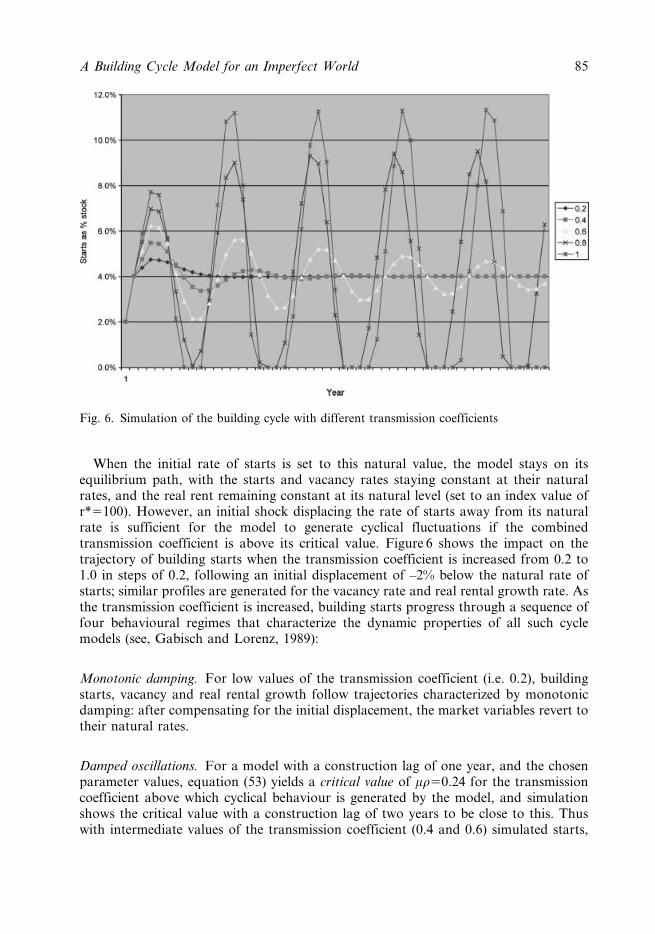
When the initial rate of starts is set to this natural value, the model stays on itsequilibrium path, with the starts and vacancy rates staying constant at their naturalrates, and the real rent remaining constant at its natural level (set to an index value ofr*5100). However, an initial shock displacing the rate of starts away from its naturalrate is sufficient for the model to generate cyclical fluctuations if the combinedtransmission coefficient is above its critical value. Figure 6 shows the impact on thetrajectory of building starts when the transmission coefficient is increased from 0.2 to1.0 in steps of 0.2, following an initial displacement of –2% below the natural rate ofstarts; similar profiles are generated for the vacancy rate and real rental growth rate. Asthe transmission coefficient is increased, building starts progress through a sequence offour behavioural regimes that characterize the dynamic properties of all such cyclemodels (see, Gabisch and Lorenz, 1989):

Monotonic damping. For low values of the transmission coefficient (i.e. 0.2), buildingstarts, vacancy and real rental growth follow trajectories characterized by monotonicdamping: after compensating for the initial displacement, the market variables revert totheir natural rates.

Damped oscillations. For a model with a construction lag of one year, and the chosenparameter values, equation (53) yields a critical value of mr50.24 for the transmissioncoefficient above which cyclical behaviour is generated by the model, and simulationshows the critical value with a construction lag of two years to be close to this. Thuswith intermediate values of the transmission coefficient (0.4 and 0.6) simulated starts,

Fig. 6. Simulation of the building cycle with different transmission coefficients


vacancy and real rental growth all exhibit damped oscillations in response to the initialdisplacement. Unless reinforced by subsequent disturbances, these oscillations die awaythrough successive cycles, the rate of dampening decreasing as the transmissioncoefficient increases. As the transmission coefficient increases, so the cycle frequencyalso increases, as predicted by equations (56) and (57).

Stable oscillations. From equation (58), with a construction lag q51 and output growthrate e50.02, the crossover point between damped and explosive cycles is reached whenthe combined transmission coefficient mr51.04. As the construction lag increases, so thecrossover point is reached with a lower transmission rate. This is because the longer thedelay, the greater the supply responses to a given demand signal, as successive periods ofdevelopment starts accumulate. Thus with the construction lag set at two years, thecrossover point is found to be 0.66, at three years it is 0.50 and at four years it is 0.40(Table 1).

When the transmission coefficient is set to its crossover value for that constructionlag, the initial displacement creates stable harmonic cycles in starts, vacancy and rentalgrowth, each oscillating around their natural rate. The period of these harmonic cyclesincreases as the construction lag increases. From equations (56) and (57), a cycle periodof 5.9 years is derived with the chosen parameter values for a one year lag; this increasesto 9.7 years with a two year lag, 13.3 years for a three year lag and 17.0 years with a fouryear lag (Table 1). As the construction lag increases from one to three years, there is aslight increase in the amplitude of the stable building cycle, but between three and fouryears there is no further increase. This means that the reduction in the transmissioncoefficient necessary to achieve a stable cycle broadly offsets the tendency to moreexplosive cycles of increased amplitude as the construction lag increases.

Explosive oscillations. For high values of the transmission coefficient (0.8 and 1.0), lyingabove the crossover point (0.66 with the construction lag q52), the simulation showshow an initial displacement generates explosive oscillations in building starts,progressively increasing in magnitude. However, these explosive oscillationseventually hit the absolute floor that starts cannot be less than zero (see equation(31)). Importantly, this is a sufficient constraint to transform an explosive cycle into onethat is stable and persistent with constant frequency, as first proposed in the non-linearbusiness cycle models developed by Hicks (1950) and Goodwin (1951), and revisited byKrugman (1996). The larger the transmission coefficient, the more quickly does the cyclehit the absolute floor, and the greater the range of the constrained oscillations that

Table 1. Stable building cycles with different construction lags

Lag(years)

Transmissioncoefficient

Cycle period(years)

Cycle amplitude(starts as % stock)

1 1.04 5.9 2.2%2 0.66 9.7 2.5%3 0.50 13.3 2.7%4 0.40 17.0 2.7%

86 R. Barras

result. Furthermore, because of the zero floor, the constrained building cycle is nolonger symmetrical around the natural starts rate, but rather its unconstrained upswingis of greater magnitude than its constrained downswing. The corresponding cycles invacancy and rental growth exhibit a similar pattern of initially explosive and thenasymmetrically constrained oscillation once the starts cycle stabilizes.

Elastic demand. The simulations presented so far all assume that the demand forbuilding space is inelastic with respect to rent. This restriction can be relaxed by allowingthe occupancy rate to vary according to equation (36). If occupiers cut down their use ofspace as rents increase, this absorbs some of the fluctuation in vacancy, in turn reducingthe volatility of induced demand for new space to be built. The strength of thisdampening effect is illustrated in Figure 7 with the transmission coefficient set to itscrossover value for a two-year construction lag, and different elasticities applied to theinverse relationship between occupancy rate and rental growth. With the occupancyelasticity set to zero, the familiar stable building cycle is generated, as the elasticity isincreased above zero, the volatility of the cycle decreases rapidly, such that an elasticityof 0.3 is sufficient to eliminate the oscillations after two cycles. What these results showis that for a persistent building cycle to be generated through the medium ofdevelopment lags there must be some ‘stickiness’ in the building occupancy rate. Thismeans that the elasticity of occupancy change with respect to rents is a fifth parameterthat determines the behaviour of the model. These results are consistent with the findingby Wheaton (1999, p. 221) that for cyclical behaviour to be generated in his model, theelasticity of space demand with respect to rents must be less than the elasticity of supply.

Composite rent adjustment. The speed of the rent adjustment process, acting as atransmission mechanism between vacancy and building starts, does not affect either the

Fig. 7. Simulation of the building cycle with variable occupancy rate starts as per cent stock


timing or amplitude of the building and vacancy cycles; however, it does affect the rentalgrowth cycle and the relationship between real rent levels and vacancy rates at differentpoints in the cycle (see Section 3.7). This can be illustrated using the simulation model, setto produce stable cycles with a two-year construction lag, and incorporating acomposite rent adjustment process as expressed by equations (27c) and (28c). Withsimple partial adjustment, the relationship between vacancy and rent levels circles aroundthe equilibrium point defined by their natural values (v*510%; r*5100); withinstantaneous full adjustment the relationship is a backward sloping straight linethrough the equilibrium point with a gradient determined by the rent adjustmentcoefficient r. Figure 8 illustrates how a composite adjustment process, with rental growthresponding to both the vacancy and rent gaps, produces intermediate vacancy-renttrajectories, with the circular path of simple partial adjustment attenuating into a narroweroval around the full adjustment line as the feedback coefficient on the rent gap increases.

5. Application to the City of London Office Market

The applicability of the model to describing the observed behaviour of property marketshas been tested by estimating some of its key equations using the annual City of Londonoffice market data introduced in Section 1. The focus is on estimating structural cyclerelationships and their parameters, rather than uncovering short-term market dynamics(see Hendershott et al., 2002, for an application to the City of London market of anerror correction model, which relates rental change to short-run changes in supply anddemand variables, adjusted by deviations from long-run market equilibrium).

As already indicated, all the variables in the estimated equations presented here areexpressed as ratios with respect to the level of occupied stock (take-up, vacancy, vacancychange, starts and completions) or rates of change (output and rents). Consequently,

Fig. 8. Simulated relationship between rents and vacancy rates with composite rent adjustment

88 R. Barras

normal rather than logged variables have been used, as there are no appreciableheteroscedasticity effects. Estimation is by OLS; the estimation period is varied tocapture the most stable model relationships (with the particularly volatile 1970s periodbeing omitted in most cases); the t-statistics for each coefficient are quoted in brackets.

5.1. Take-up and Net Absorption

As already indicated in Section 1, take up of space in the market is a directly measuredquantity, unlike net absorption, and equation (11) shows that the rate of take up can beexpressed as a function of the output growth rate, the occupancy rate and the turnoverrate. Furthermore, if it is assumed that the occupancy rate varies with marketconditions, as expressed in equation (36), then rental change can be introduced into thetake-up equation to act as a proxy for changes in the occupancy rate.

On this basis the rate of take up in the City, illustrated in Figure 1, has been estimatedover the period 1984–2004, with London GDP growth found to be a suitable indicatorof demand growth:

ut~6:13z0:725DYt=Yt�1�0:029Drt�5:97dum02

12:20ð Þ 4:37ð Þ �1:81ð Þ �4:44ð Þ

adjR2~0:608; n~21 1984� 2004ð Þ; DW~2:30:

ð59Þ

To achieve this level of fit, it was necessary to introduce a dummy for the year 2002,when City take up collapsed to its lowest recorded level relative to occupied stock, inresponse to the shock of the stock market crash of 2001–02. Estimation of the equivalentequation using net absorption rather than take up produced no significant coefficients.

This equation offers a plausible explanation for the drivers of the take up rate. Theconstant suggests a turnover rate of just over 6% of occupied stock, boosted by the netabsorption generated by London output growth, and moderated by the impact of realrental change. However, the estimated negative impact of rental change on demandappears quite weak, confirming that there is considerable inelasticity in the occupiermarket, because of long leases and high moving costs that hamper its potential to dampendown the building cycle through variations in the occupancy rate (see Section 4.4).

The extent of demand inelasticity can be illustrated by separately estimating theoccupancy rate as an inverse function of real rental growth, according to equation (36),using floor space per employee in City financial and business services as the measure ofoccupancy rate

at~209:2� 1:493 Drt�2=rt�3ð Þ

ð80:3Þ �7:22ð Þ

adjR2~0:690; n~24 1980� 2003ð Þ; DW~1:25:

ð60Þ

There is an inverse relationship between the occupancy rate and real rental change,but lagged by two years as an indicator of the stickiness of the demand response. Theconstant yields an average natural occupancy rate a* of 209 square feet per employee inthe City over the estimation period.


5.2. Vacancy Change

The vacancy change relationship in the City, illustrated in Figure 2, has been estimatedfrom equation (35) over the full period 1971–2004 as

Dvt~6:21z1:009ct�0:821ut�0:318vt�1

3:54ð Þ 5:40ð Þ �3:44ð Þ �3:89ð Þ

adjR2~0:548; n~34 1971� 2004ð Þ; DW~1:72:

ð61Þ

This long-run accounting relationship captures the determinants of vacancychange reasonably well, though there is inevitably a considerable amount of unex-plained short-term variation due to the erratic nature of the dependent variable. Theequation shows vacancy to be boosted by the rate of completions, with a coefficientvery close to the expected value of unity, and reduced by the rate of take-up, with acoefficient less than unity, reflecting some impact of the turnover as distinct fromnet absorption component of take-up. There is also a self-correcting negative feedbackfrom vacancy level to vacancy change: the higher the level, the more likely it is tofall.

Fig. 9. City of London rent-vacancy relationship (1974–2004)

90 R. Barras

5.3. Rent Adjustment

Alternative rent adjustment equations have been estimated for the City, according tothe full, partial and composite formulations set out in equations (27a) to (27c). Figure 3shows a strong inverse relationship between real rental growth and vacancy level in theCity, whereas the corresponding plot of real rent levels versus vacancy presented inFigure 9 follows a broad oval trajectory around the equilibrium point, indicatingweak feedback from rent levels to rental growth as illustrated in Figure 8 using thesimulation model. This reflects the historic tendency for each supply cycle in the City todrive the average level of real rents to successive lower levels. The regression estimatesfor the City confirm these observations: the partial adjustment equation is muchstronger than the full adjustment form, and the rent gap term is insignificant in thecomposite adjustment equation (though estimates for some other UK and Europeanoffice markets do show the negative feedback of rent levels on rental growth to besignificant).

The partial rent adjustment equation has been estimated over the period 1982–2004 as

Drt=rt�1~22:63� 1:878vt

7:49ð Þ �8:58ð Þ

adjR2~0:767; n~23 1982� 2004ð Þ; DW~1:61:

ð62Þ

This version relates proportionate real rental change Drt/rt-1 to the vacancy rate vt atthe end of the period; it gives a considerably stronger model than that fitted to thevacancy rate vt-1 at the beginning of the period, which is the typical rent adjustmentrelationship as incorporated in equation (27b). Owing to the lag structure of the model,the estimated form of the rent adjustment equation does not create a problem of co-determination between rents and vacancy. It yields estimates of 1.88 for the rent

adjustment coefficient r, and 12.1% for the natural vacancy rate v* at which rentalgrowth is zero in the City. This natural vacancy rate is calculated with respect tooccupied space; the equivalent rate measured against total stock is 10.5%. Estimates ofthe natural vacancy rate in other UK and European office markets are typically lowerreflecting the tendency to over-supply in the City market that maintains average vacancyrates at relatively high levels.

5.4. Development Supply

As for rental growth, the development supply relationship has also been formulatedusing alternative adjustment processes, as set out in equations (28a) to (28c). Unlike therent adjustment equations, all three versions of the development supply equationproduce significant relationships when estimated for the City. These equations provideestimates for the natural rate of starts and natural rent level on the simplifyingassumption that both are constant (see Section 3.6).

Corresponding to rental growth equation (62), the partial adjustment develop-ment relationship, illustrated in Figure 4, has been estimated over the shortened period1985–2004 as


st~4:07z0:160 Drt=rt�2ð Þ�1

11:65ð Þ

6:71ð Þ

adjR2~0:699; n~20 1985� 2004ð Þ; DW~1:06:

ð63Þ

This version of the partial adjustment equation expresses the rate of developmentstarts as a function of lagged real rental growth; again, this gives a considerably strongermodel than the unlagged relationship assumed in equation (28b). The constant inthe equation corresponds to a fixed natural rate of starts; the equation was alsoexpanded to include an index of construction costs and the interest rate, to allowthe natural starts rate to vary with development costs, but as is usually found whenestimating such development equations neither variable was found to be significant(see Section 2).

For comparison with the simulation model, equation (63) yields estimates of 4.1% forthe constant natural rate of starts s* around which the building cycle oscillates, and 0.16for the development reaction coefficient m:

N The estimated natural rate of starts of 4.1% in the City is reasonably close to theequilibrium value of 4.7% that can be obtained from model equation (49), allow-ing for expectations of future growth. This equilibrium value is derived by usingestimated parameter values of 12.1% for the natural vacancy rate v* and 2.6 yearsfor the average construction lag q (see below), together with an average outputgrowth rate of 2.7% per annum for London GDP over the period, and an averageCity office depreciation rate previously estimated to be around 1.2% per annum(Barras and Clark, 1996).

N The product of the estimated rent adjustment and development reaction coefficientsyields a combined transmission coefficient mr with a value of 0.30. Although the lagstructure of the individual equations differs from that adopted in model equations(27b) and (28b), their combined effect is the same one year lag between the relativevacancy signal and development starts as that derived in equation (29). The estimatedvalue of the transmission coefficient is above the critical value of 0.24 derived fromequation (53) but below the crossover point with a construction lag of two to threeyears (see Table 1), therefore lying in the range in which damped cycles are generated.This suggests that the persistent severity of the building cycle in the City and othersimilar office markets is the result of occasional shocks, which destabilize thetendency for the market to return towards equilibrium through a sequence of dampedcycles.

An improved development supply equation, with better adjusted R2 and lessautocorrelation, was obtained using a composite adjustment equation, similar in form toequation (28c) but with a different lag structure combining the unlagged real rent levelwith lagged real rental growth,

92 R. Barras

st~� 0:498z0:097 Drt�1=rt�2ð Þz0:035rt

�0:57ð Þ 5:11ð Þ 5:41ð Þ

adjR2~0:883; n~20 1985� 2004ð Þ; DW~2:18:

ð64Þ

This equation yields an estimate of 0.27 for the feedback coefficient b in the compositeadjustment process, and an index value of 131 for the constant level of natural rent r*over the estimation period (with real City rents indexed to a value of 100 in 1965), basedupon the value of the natural rate of starts derived from equation (63). The derivedrelationship suggests that developers in the City respond both to rental change, feedingexpectations of improving or worsening market conditions, and the prevailing rent level,indicating current levels of development profitability.

Again, the addition of development cost variables caused no significant improve-ment to equation (64), and neither did the addition of the real interest rate, a potentialinfluence on the natural rent level acting as a user cost of capital (see Hendershott et al.,1999, for an attempt to construct a natural rent series for the City). Equivalentversions of equations (63) and (64) were also estimated using real capital valuesrather than real rents; with both formulations, rents appeared to be the strongertrigger for development activity. Current output growth was also tried in each equationas a proxy for developer expectations about future demand growth, but in neither casewas found to be significant, confirming the assumption of myopic pricing adopted forthe model.

5.5. Construction Delay

The construction lag between the rates of starts and completions in the City, asillustrated in Figure 5, has been estimated from equation (32) over the period 1975–2004 as

ct~0:317z0:374st�2z0:618st�3

0:59ð Þ 2:32ð Þ 3:84ð Þ

adjR2~0:651; n~30 1975� 2004ð Þ; DW~2:46:

ð65Þ

The estimated equation confirms what is apparent from Figure 5: the crucialconstruction lag between starts and completions that drives the building cycle is betweentwo and three years in the City. The coefficients on the lagged (–2) and lagged (–3) ratesof starts add to 0.992, very close to the expected long-run average of one; a weightedaverage of the two coefficients suggests an average lag of 2.6 years.

By interpolation from Table 1, an average construction lag of 2.6 years implies abuilding cycle period of some 11.9 years according to the simulation model. This modelestimate applies when the transmission coefficient is at its crossover point; if it is belowthat point, the cycle period is longer (see Section 4.4). These model results correspondswell with the observed starts cycle in the City: with peaks in 1973, 1988 and 2001 it has


an average period of around 14 years, which is higher than the model estimate at thecrossover point but consistent with having an estimated transmission coefficient belowthe crossover point for this average lag.

6. Conclusions

Strong cyclical movements in building activity, vacancy and rents characterize many realestate markets, most notably large mature office markets such as the City of London. Toreplicate these cycles, a mathematical model of the building cycle has been constructedwith the following characteristics:

N Cyclical fluctuations are generated endogenously around an equilibrium growthpath that determines the natural rate of building starts as a function of the sum of theeconomic growth rate and building depreciation rate, inflated to allow for a bufferstock of vacant space and for the expected growth of demand during the constructionperiod.

N In addition to the natural rate of starts, the market clearing equilibrium at each pointon the growth trajectory is defined by a natural occupancy rate, vacancy rate, realrent level and property yield.

N The dynamic behaviour of the model in response to an initial disturbance awayfrom the equilibrium growth path is determined by lags in three adjustment pro-cesses: the demand response to changes in rents, mediated through shifts in theoccupancy rate; the development response to changes in demand, mediated througha rent adjustment process; and the construction delay in translating developmentstarts into completions.

N Under the simplifying assumptions of inelastic occupier demand plus single lags inthe development response and construction delay, an analytical solution to the modelis derived as a second order difference equation in the rate of building starts; longerlags and elastic demand generate higher order non-linear difference equations thatrequire simulation to demonstrate their cyclical properties.

N Cyclical behaviour depends upon the values of five key model parameters: the outputgrowth rate; the depreciation rate; the construction lag; the combined transmissioncoefficient linking vacancy to development starts; and the demand elasticity on theoccupancy rate.

N The higher the transmission coefficient, the more explosive the building cycle fluc-tuations that are generated, and the higher their frequency; the longer theconstruction lag, the longer the cycle period and the more explosive it is for a givenvalue of the transmission coefficient.

N The more elastic the occupancy rate with respect to rental change, the more thebuilding cycle is dampened down as some of the cyclical tendency created by the lagstructure is absorbed by the demand side of the market.

The model has been fitted to data for the City of London office market, yieldingestimates for key parameters that are consistent with its observed cyclical behaviour.Work is underway to test the model on data for other major office markets in Europe,the US and Asia.

94 R. Barras

References

Antwi, A. and Henneberry, J. (1995) Developers, non-linearity and asymmetry in the developmentcycle, Journal of Property Research, 12(3), 217–39.

Ball, M., Lizieri, C. and MacGregor, B.D. (1998) The Economics of Commercial Property

Markets. Routledge, London.

Barras, R. (1983) A simple theoretical model of the office development cycle, Environment and

Planning A, 15, 1381–94.

Barras, R. (1994) Property and the economic cycle: building cycles revisited, Journal of Property

Research, 11, 183–97.

Barras, R. (2001) Building investment is a diminishing source of economic growth, Journal of

Property Research, 18(4), 279–308.

Barras, R. (forthcoming) Building Cycles and Urban Development. Blackwell, Oxford.

Barras, R. and Clark, P. (1996) Obsolescence and performance in the Central London officemarket, Journal of Property Valuation and Investment, 14(4), 63–78.

Barras, R. and Ferguson, D. (1987) Dynamic modeling of the building cycle: 1. theoreticalframework, Environment and Planning A, 19, 353–67.

Bischoff, C.W. (1970) A model of nonresidential construction in the United States, American

Economic Review: Papers and Proceedings, 60(2), 10–7.

Chenery, H.B. (1952) Overcapacity and the acceleration principle, Econometrica, 20(1), 1–28.

Dokko, Y., Edelstein, R.H., Lacayo, A.J. and Lee, D.C. (2001) Real estate income and valuecycles, in S.J. Brown and C.H. Liu (Eds) A Global Perspective on Real Estate Cycles. Kluwer,Boston.

Dore, M.H.I. (1993) The Macroeconomics of Business Cycles. Blackwell, Oxford.

Elaydi, S.N. (1996) An Introduction to Difference Equations. Springer-Verlag, New York.

Gabisch, G. and Lorenz, H.-W. (1989) Business Cycle Theory. Springer-Verlag, Berlin.

Goodwin, R.M. (1951) The nonlinear accelerator and the persistence of business cycles,Econometrica, 19(1), 1–17.

Goodwin, R.M. (1967) A growth cycle, in C.H. Feinstein (Ed.) Socialism, Capitalism and

Economic Growth, 54–8, Cambridge University Press, Cambridge.

Grenadier, S.R. (1995) The persistence of real estate cycles, Journal of Real Estate Finance and

Economics, 10, 95–119.

Hekman, J.S. (1985) Rental price adjustment and investment in the office market, Journal of the

American Real Estate and Urban Economics Association, 13(1), 32–47.

Hendershott, P.H. (1995) Real effective rent determination: evidence from the Sydney officemarket, Journal of Property Research, 12(2), 127–35.

Hendershott, P.H., Lizieri, C.M. and Matysiak, G.A. (1999) The workings of the London officemarket, Real Estate Economics, 27(2), 365–87.

Hendershott, P.H., MacGregor, B.D. and Tse, R.Y.C. (2002) Estimation of the rental adjustmentprocess, Real Estate Economics, 30(2), 165–83.

Hicks, J.R. (1950) A Contribution to the Theory of the Trade Cycle. Clarendon Press, Oxford.

Kaldor, N. (1961) Capital accumulation and economic growth, in F.A. Lutz and D.C. Hague(Eds) The Theory of Capital, Macmillan, London, pp. 177–222.

Kalecki, M. (1937) A theory of the business cycle, Review of Economic Studies, 4, 77–97.

Key, T., MacGregor, B.D., Nanthakumaran, N. and Zarkesh, F. (1994) Economic Cycles andProperty Cycles, ‘Understanding the Property Cycle’ Main Report, London, RoyalInstitution of Chartered Surveyors.

Kling, J.L. and McCue, T.E. (1987) Office building investment and the macroeconomy: empiricalevidence, 1973–1985, Journal of the American Real Estate and Urban Economics Association,15(3), 234–55.

Krugman, P. (1996) The Self-Organizing Economy. Blackwell, Oxford.


Kummerow, M. (1999) A system dynamics model of cyclical office oversupply, Journal of Real

Estate Research, 18(1), 233–55.Kydland, F.E. and Prescott, E.C. (1982) Time to build and aggregate fluctuations, Econometrica,

50(6), 1345–70.McDonald, J.F. (2000) Rent, vacancy and equilibrium in real estate markets, Journal of Real

Estate Practice and Education, 3(1), 55–69.McDonald, J.F. (2002) A survey of econometric models of office markets, Journal of Real Estate

Literature, 10(2), 223–42.Rosen, K.T. (1984) Towards a model of the office building sector, Journal of the American Real

Estate and Urban Economics Association, 12(3), 261–9.Samuelson, P.A. (1939) Interaction between the multiplier analysis and the principle of

acceleration, Review of Economic Statistics, 21, 75–8.Sivitanides, P.S. (1997) The rent adjustment process and the structural vacancy rate in the

commercial real estate market, Journal of Real Estate Research, 13(2), 195–209.Smith, L.B. (1974) A note on the rent adjustment mechanism for rental housing, American

Economic Review, 64, 478–81.Strogatz, S.H. (1994) Nonlinear Dynamics and Chaos. Perseus Books, Cambridge MA.Tsolacos, S., Keogh, G. and McGough, T. (1998) Modelling use, investment and development in

the British office market, Environment and Planning A, 30, 1409–27.Tsolacos, S. and McGough, T. (1999) Rational expectations, uncertainty and cyclical activity in

the British office market, Urban Studies, 36(7), 1137–49.Wheaton, W.C. (1987) The cyclic behaviour of the national office market, Journal of the American

Real Estate and Urban Economics Association, 15(4), 281–99.Wheaton, W.C. (1999) Real estate ‘cycles’: some fundamentals, Real Estate Economics, 27(2),

209–30.Wheaton, W.C. and Torto, R.G. (1990) An investment model of the demand and supply for

industrial real estate, Journal of the American Real Estate and Urban Economics Association,18(4), 530–47.

Wheaton, W.C., Torto, R.G. and Evans, P. (1997) The cyclic behaviour of the Greater Londonoffice market, Journal of Real Estate Finance and Economics, 15(1), 77–92.

96 R. Barras

a building cycle model for an imperfect world

Documents

late 1980s early 1990s

real estate finance

american real estate

repeated exogenous shocks

real estate markets

composite adjustment process

composite rent adjustment

real estate economics