a brief review of tests for...
TRANSCRIPT
American Journal of Theoretical and Applied Statistics 2016; 5(1): 5-12
Published online January 27, 2016 (http://www.sciencepublishinggroup.com/j/ajtas)
doi: 10.11648/j.ajtas.20160501.12
ISSN: 2326-8999 (Print); ISSN: 2326-9006 (Online)
Review Article
A Brief Review of Tests for Normality
Keya Rani Das1, *
, A. H. M. Rahmatullah Imon2
1Department of Statistics, Bangabandhu Sheikh Mujibur Rahman Agricultural University, Gazipur, Bangladesh 2Department of Mathematical Sciences, Ball State University, Muncie, IN, USA
Email address: [email protected] (K. R. Das), [email protected] (A. H. M. R. Imon)
To cite this article: Keya Rani Das, A. H. M. Rahmatullah Imon. A Brief Review of Tests for Normality. American Journal of Theoretical and Applied Statistics.
Vol. 5, No. 1, 2016, pp. 5-12. doi: 10.11648/j.ajtas.20160501.12
Abstract: In statistics it is conventional to assume that the observations are normal. The entire statistical framework is
grounded on this assumption and if this assumption is violated the inference breaks down. For this reason it is essential to check
or test this assumption before any statistical analysis of data. In this paper we provide a brief review of commonly used tests for
normality. We present both graphical and analytical tests here. Normality tests in regression and experimental design suffer from
supernormality. We also address this issue in this paper and present some tests which can successfully handle this problem.
Keywords: Power, Empirical Cdf, Outlier, Moments, Skewness, Kurtosis, Supernormality
1. Introduction
In all branches of knowledge it is necessary to apply
statistical methods in a sensible way. In the literature statistical
misconceptions are conventional. The most commonly used
statistical methods are correlation, regression and
experimental design. But all of them are based on one basic
assumption, that the observation follows normal (Gaussian)
distribution. So it is assumed that the populations from where
the samples are collected are normally distributed. For this
reason the inferential methods require checking the normality
assumption.
In the last hundred years, attitudes towards the assumption
of a Normal distribution in statistical models have varied from
one extreme to another. To quote Pearson (1905) ‘Even
towards the end of the nineteenth century not all were
convinced of the need for curves other than normal.’ By the
middle of this century Geary (1947) made this comment
`Normality is a myth; there never was and never will be a
normal distribution.' This might be an overstatement, but the
fact is that non-Normal distributions are more prevalent in
practice than formerly assumed.
Gnanadesikan (1977) pointed out, `the effects on classical
methods of departure from normality are neither clearly nor
easily understood.' Nevertheless, evidence is available that
shows such departures can have unfortunate effects in a
variety of situations. In regression problems, the effects of
departure from normality in estimation were studied by Huber
(1973). He pointed out that, under non-Normality it is difficult
to find necessary and sufficient conditions such that all
estimates of the parameters are asymptotically normal. In
testing hypotheses, the effect of departure from normality has
been investigated by many statisticians. A good review of
these investigations is available in Judge et al. (1985). When
the observations are not normally distributed, the associated
normal and chi-square tests are inaccurate and consequently
the t and F tests are not generally valid in finite samples.
However, they have an asymptotic justification. The sizes of t
and F tests appear fairly robust to deviation from normality
[see Pearson and Please (1975)]. This robustness of validity is
obviously an attractive property, but it is important to
investigate the response of tests' power as well as size to
departure from normality. Koenker (1982) pointed out that the
power of t and F tests is extremely sensitive to the
hypothesized distribution and may deteriorate very rapidly as
the distribution becomes long-tailed. Furthermore, Bera and
Jarque (1982) have found that homoscedasticity and serial
independence tests suggested for normal observations may
result in incorrect conclusions under non-normality. It may be
also essential to have proper knowledge of observations in
prediction and in confidence limits of predictions. Most of the
standard results of this particular study are based on the
normality assumption and the whole inferential procedure
may be subjected to error if there is a departure from this. In

6 Keya Rani Das and A. H. M. Rahmatullah Imon: A Brief Review of Tests for Normality
all, violation of the normality assumption may lead to the use
of suboptimal estimators, invalid inferential statements and
inaccurate predictions. So for the validity of conclusions we
must test the normality assumption. The main objective of this
paper is to accumulate the procedures by which we can
examine normality assumption. There is now a very large
body of literature on tests for Normality and many textbooks
contain sections on the topic. Mardia (1980) and D'Agostino
(1986) gave excellent reviews of these tests. We consider in
this paper a few of them which are selected mainly for their
good power properties. The prime objective of this paper is to
distinguish different types of normality tests for different areas
of statistics. For the moment practitioners indiscriminantly
apply normality tests. But in this paper we will show tests
developed for univariate independent samples should not be
readily applied for regression and design of experiments
because of the supernormality problem. We try to categorize
the normality tests in several classes although we recognize
the fact that there are many more tests (not considered here)
which may not come under these categories. This consists of
both graphical plots and analytical test procedures.
2. Graphical Method
Any statistical analysis enriched by including appropriate
graphical checking of the observation. To quote Chambers et
al. (1983) ‘Graphical methods provide powerful diagnostic
tools for confirming assumptions, or, when the assumptions
are not met, for suggesting corrective actions. Without such
tools, confirmation of assumptions can be replaced only by
hope.’ Some statistical plots such as scatter plots, residual
plots are advised for checking or diagnostic statistical method.
For goodness of fit and distribution curve fitting graphical
plots are necessary and give ideas about pattern. Existing
testing methods give an objective decision of normality. But
these do not provide general hint about cause of rejecting a
null hypothesis. So, we are interested to present different types
plot for normality checking as well as various testing
procedures of it. Generally histograms, stem-and-leaf plots,
box plots, percent-percent (P-P) plots, quantile-quantile (Q-Q)
plots, plots of the empirical cumulative distribution function
and other variants of probability plots have most application
for normality assumption checking.
2.1. Histogram
The easiest and simplest graphical plot is the histogram.
The frequency distribution in which the observed values are
plotted against their frequency, states a visual estimation
whether the distribution is bell shaped or not. At the same,
time it provides indication about insights gap in the data and
outliers. Also it gives idea about skewness or symmetry.
Data that can be represented by this type of ideal,
bell-shaped curve as shown in the first graph are said to have a
normal distribution or to be normally distributed. Of course
for the second graph the data are not normally distributed.
Figure 1. Histogram shows the data are normally distributed.
Figure 2. Histogram shows the data are not normally distributed.
2.2. Stem-and-Leaf Plot
Stem-and-leaf display states identical knowledge as like
histogram but observation appeared with their identity seems
they do not lose their any information about original data. Like
histogram, they show frequency of observations along with
median value, highest and lowest values of the distribution,
other sample percentiles from the display of data. There is a
“stem” and a “leaf” for each values where the stems depicts a
set of bins in which leaves are grouped and these leaves reflect
bars like histogram.
Figure 3. Stem-and-leaf plot shows the data are not normally distributed.
The above stem-and-leaf plot of marks obtained by the
students clearly shows that the data are not normally
distributed.
American Journal of Theoretical and Applied Statistics 2016; 5(1): 5-12 7
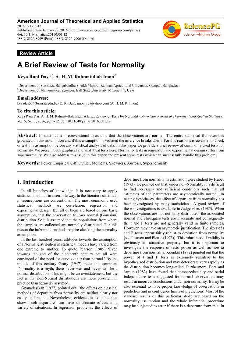
2.3. Box-and-Whisker Plot
It has another name as five number summary where it needs
first quartile, second quartile or median, third quartile,
minimum and maximum values to display. Here we try to plot
our data in a box whose midpoint is the sample median, the top
of the box is the third quartile (Q3) and the bottom of the box
is the first quartile (Q1). The upper whisker extends to this
adjacent value - the highest data value within the upper limit =
Q3 + 1.5 IQR where the inter quartile range IQR is defined as
IQR = Q3-Q1. Similarly the lower whisker extends to this
adjacent value - the lowest value within the lower limit = Q1-
1.5 IQR.
Figure 4. Box-and-Whisker plot shows the data are not normally distributed.
We consider an observation to be unusually large or small
when it is plotted beyond the whiskers and they are treated as
outliers. By this plot we can get clear indication about
symmetry of data set. At the same time it gives idea about
scatteredness of observations. Thus the normality pattern of
the data is understood by this plot as well.
The box plot presented in Figure 1 is taken from Imon and
Das (2015). This plot clearly shows non-normal pattern of the
data. It contains outlier and the data are not even symmetric
which is, in fact, skewed to the right.
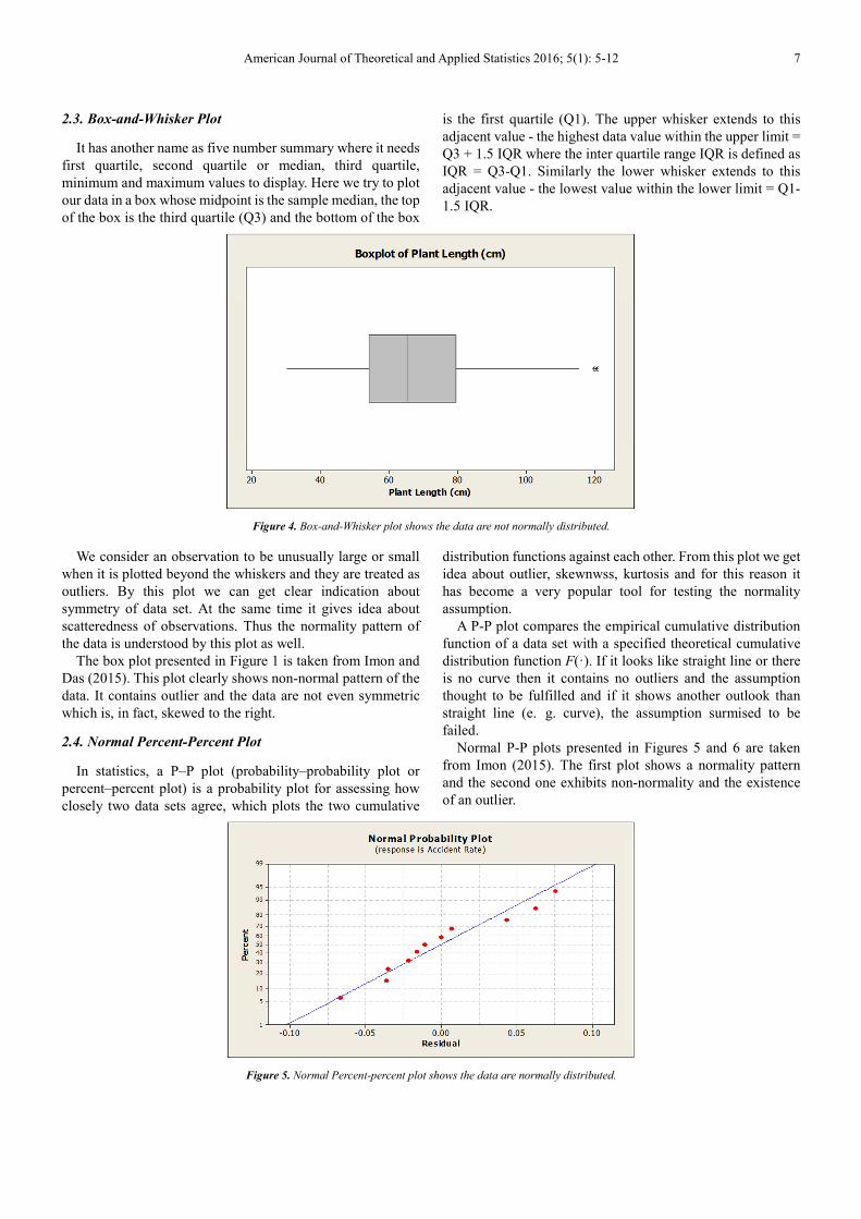
2.4. Normal Percent-Percent Plot
In statistics, a P–P plot (probability–probability plot or
percent–percent plot) is a probability plot for assessing how
closely two data sets agree, which plots the two cumulative
distribution functions against each other. From this plot we get
idea about outlier, skewnwss, kurtosis and for this reason it
has become a very popular tool for testing the normality
assumption.
A P-P plot compares the empirical cumulative distribution
function of a data set with a specified theoretical cumulative
distribution function F(·). If it looks like straight line or there
is no curve then it contains no outliers and the assumption
thought to be fulfilled and if it shows another outlook than
straight line (e. g. curve), the assumption surmised to be
failed.
Normal P-P plots presented in Figures 5 and 6 are taken
from Imon (2015). The first plot shows a normality pattern
and the second one exhibits non-normality and the existence
of an outlier.
Figure 5. Normal Percent-percent plot shows the data are normally distributed.

8 Keya Rani Das and A. H. M. Rahmatullah Imon: A Brief Review of Tests for Normality
Figure 6. Normal percent-percent plot shows the data are non-normal.
2.5. Normal Quantile-Quantile Plot
A quantile-quantile(Q-Q)plot compares the quantiles of a
data distribution with the quantiles of a standardized
theoretical distribution from a specified family of distributions.
A normal Q-Q plot is that which we can shaped by plotting
quantiles of one distribution versus quantiles of normal
distribution. When quantiles of two distributions are met,
plotted dots face with the line y = x. If it shows curve size with
slope rising from left to right, it indicates the data distribution
is skewed to the right and curve size with slope decreasing
from left to right, it exposes skewness is to the left for the
distribution. By investigating in normal probability paper, a
Q-Q plot can easily be produced by hand. The abscissa on
probability paper is scaled in proportionally to the expected
quantiles of a standard normal distribution so that a plot of (p,
��� (p)) is linear. The abscissa limits typically run from
0.0001 to 0.9999. The vertical scale is linear and does not
require that the data be standardized in any manner; also
available is probability paper that is scaled logarithmically on
the y-axis for use in determining whether data is lognormally
distributed. On probability paper, the pairs ( �� , ���� ) are
plotted. For plots done by hand, the advantage of Q-Q plots
done on normal probability paper is that percentiles and
cumulative probabilities can be directly estimated, and,
���(��) need not be obtained to create the plot.
There is a great area of confusion between P-P plot and Q-Q
plot and sometimes people think that they are synonymous.
But there are three important differences in the way P-P plots
and Q-Q plots are constructed and interpreted:
� The construction of a Q-Q plot does not require that the
location or scale parameters of F(·) be specified. The
theoretical quantiles are computed from a standard
distribution within the specified family. A linear point
pattern indicates that the specified family reasonably
describes the data distribution, and the location and scale
parameters can be estimated visually as the intercept and
slope of the linear pattern. In contrast, the construction of
a P-P plot requires the location and scale parameters of
F(·) to evaluate the cdf at the ordered data values.
� The linearity of the point pattern on a Q-Q plot is
unaffected by changes in location or scale. On a P-P plot,
changes in location or scale do not necessarily preserve
linearity.
� On a Q-Q plot, the reference line representing a
particular theoretical distribution depends on the
location and scale parameters of that distribution, having
intercept and slope equal to the location and scale
parameters. On a P-P plot, the reference line for any
distribution is always the diagonal line y = x.
Consequently, you should use a Q-Q plot if your objective
is to compare the data distribution with a family of
distributions that vary only in location and scale, particularly
if you want to estimate the location and scale parameters from
the plot.
An advantage of P-P plots is that they are discriminating in
regions of high probability density, since in these regions the
empirical and theoretical cumulative distributions change
more rapidly than in regions of low probability density. For
example, if you compare a data distribution with a particular
normal distribution, differences in the middle of the two
distributions are more apparent on a P-P plot than on a Q-Q
plot.
2.6. Empirical Cumulative Distribution Function Plot
An empirical CDF plot performs a similar function as a
probability plot. However, unlike a probability plot, the
empirical CDF plot has scales that are not transformed and the
fitted distribution does not form a straight line, rather it yields
an S-shape curve under normality. The empirical cumulative
probabilities close to this S-shape curve satisfies the normality
assumption.
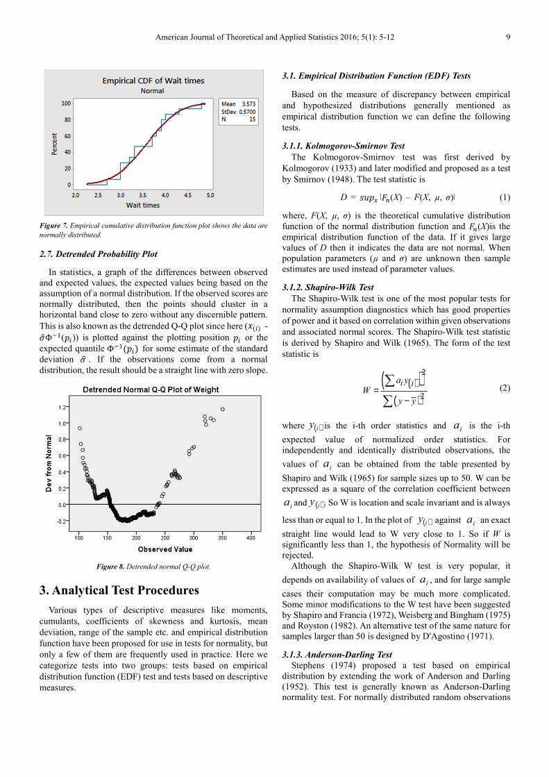
American Journal of Theoretical and Applied Statistics 2016; 5(1): 5-12 9
Figure 7. Empirical cumulative distribution function plot shows the data are
normally distributed.
2.7. Detrended Probability Plot
In statistics, a graph of the differences between observed
and expected values, the expected values being based on the
assumption of a normal distribution. If the observed scores are
normally distributed, then the points should cluster in a
horizontal band close to zero without any discernible pattern.
This is also known as the detrended Q-Q plot since here (���� -
��(��)) is plotted against the plotting position �� or the
expected quantile ������ for some estimate of the standard
deviation . If the observations come from a normal
distribution, the result should be a straight line with zero slope.
Figure 8. Detrended normal Q-Q plot.
3. Analytical Test Procedures
Various types of descriptive measures like moments,
cumulants, coefficients of skewness and kurtosis, mean
deviation, range of the sample etc. and empirical distribution
function have been proposed for use in tests for normality, but
only a few of them are frequently used in practice. Here we
categorize tests into two groups: tests based on empirical
distribution function (EDF) test and tests based on descriptive
measures.
3.1. Empirical Distribution Function (EDF) Tests
Based on the measure of discrepancy between empirical
and hypothesized distributions generally mentioned as
empirical distribution function we can define the following
tests.
3.1.1. Kolmogorov-Smirnov Test
The Kolmogorov-Smirnov test was first derived by
Kolmogorov (1933) and later modified and proposed as a test
by Smirnov (1948). The test statistic is
D = ��� ǀ��(X) – F(X, µ, σ)ǀ (1)
where, F(X, µ, σ) is the theoretical cumulative distribution
function of the normal distribution function and ��(X)is the
empirical distribution function of the data. If it gives large
values of D then it indicates the data are not normal. When
population parameters (µ and σ) are unknown then sample
estimates are used instead of parameter values.
3.1.2. Shapiro-Wilk Test
The Shapiro-Wilk test is one of the most popular tests for
normality assumption diagnostics which has good properties
of power and it based on correlation within given observations
and associated normal scores. The Shapiro-Wilk test statistic
is derived by Shapiro and Wilk (1965). The form of the test
statistic is
( )( )( )
2
2
i ia yW
y y=
−
∑
∑ (2)
where ( )iy is the i-th order statistics and ia is the i-th
expected value of normalized order statistics. For
independently and identically distributed observations, the
values of ia can be obtained from the table presented by
Shapiro and Wilk (1965) for sample sizes up to 50. W can be
expressed as a square of the correlation coefficient between
ia and ( )iy . So W is location and scale invariant and is always
less than or equal to 1. In the plot of ( )iy against ia an exact
straight line would lead to W very close to 1. So if W is
significantly less than 1, the hypothesis of Normality will be
rejected. Although the Shapiro-Wilk W test is very popular, it
depends on availability of values of ia , and for large sample
cases their computation may be much more complicated.
Some minor modifications to the W test have been suggested
by Shapiro and Francia (1972), Weisberg and Bingham (1975)
and Royston (1982). An alternative test of the same nature for
samples larger than 50 is designed by D'Agostino (1971).
3.1.3. Anderson-Darling Test
Stephens (1974) proposed a test based on empirical
distribution by extending the work of Anderson and Darling
(1952). This test is generally known as Anderson-Darling
normality test. For normally distributed random observations

10 Keya Rani Das and A. H. M. Rahmatullah Imon: A Brief Review of Tests for Normality
( )iy with mean µ and variance 2σ , the Anderson-Darling
test statistic is given by
( ) ( ){ }12 1
2
ˆ ˆ2 1 log 10.75 2.25
1
n
i n ii
i z z
A nn nn
+ −=
− −
= − + + +
∑ (3)
Where ( )( )[ ]σµ ˆ/ˆˆ −Φ=ii
yz and ( )•Φ is the
distribution function of an N (0,1) random variable. Stephens
(1974) provided the percentage points for this test.
3.2. Tests Based on Descriptive Measures
Fisher (1930) proposed using cumulants. Using his result,
Pearson (1930) obtained the first four moments of the
sampling distribution of skewness and kurtosis, under the null
hypothesis of normality. He used those results to develop
criteria for testing normality by using sample values of
coefficients of skewness and kurtosis separately. The ratio of
mean deviation to standard deviation [see Geary (1935)] and
ratio of sample range to standard deviation [see David, Hartley,
and Pearson (1954)] were also proposed for the same purpose.
Based on moments the most popular tests are
D’Agostino-Pearson Omnibus test and Jarqua-Bera test.
3.2.1. D’Agostino-Pearson Omnibus Test
To assessing the symmetry or asymmetry generally
skewness is measured and to evaluate the shape of the
distribution kurtosis is overlooked. D’Agostino-Pearson
(1973) test standing on the basis of skewness and kurtosis test
and these are also assessing through moments. The DAP
statistic is
�� = ������� + ������ (4)
where Z ����� and Z( �� ) are the normal approximation
equivalent to ��� and �� are sample skewness and kurtosis
respectively. This statistic follows a chi-squared distribution
with two degrees of freedom if the population is from normal
distribution. A large value of �� leads to the rejection of the
normality assumption.
3.2.2. Jarqua-Bera Test
The Jarqua-Bera test was originally proposed by Bowman
and Shenton (1975). They combined squares of normalized
skewness and kurtosis in a single statistic as follows
JB = [n / 6] [ 2 2( 3)S K+ − / 4] (5)
This normalization is based on normality since S = 0 and K
= 3 for a normal distribution and their asymptotic variances
are 6/n and 24/n respectively. Hence under normality the JB
test statistic follows also a chi-squared distribution with two
degrees of freedom. A significantly large value of JB leads to
the rejection of the normality assumption.
4. Supernormality and Rescaled
Moments Test
Test procedures discussed so far can be applied for testing
normality of the distribution from which we have collected the
observations. Here the normality test is employed on an
observed data set. But in regression and design problems,
since the true errors are unobserved, it is a common practice to
use the residuals as substitutes for them in tests for normality.
The residuals have several drawbacks which have made
statisticians question [see Cook and Weisberg (1982)] whether
they can be used as proper substitutes for the true errors or not.
In testing normality, all test statistics have been designed on
the basis of independent and identically distributed random
observations. An immediate problem of using residuals in
them is that even when the true errors are independent, their
corresponding residuals are always correlated. Residuals also
have the problem of not possessing constant variance while
the true errors do so. They also have the disadvantage that
their probability distribution is always closer to normal form
than is the probability distribution of the true errors, when the
errors are not normal. This problem is generally known as the
supernormality effect of the residuals.
Since the question has been raised about the use of residuals
as proper estimates of the errors because of supernormality,
this practice of using them in test procedures looks
questionable. But, most important, the induced normality of
the residuals makes a test of normality of the true errors based
on residuals logically very weak.
Figure 9. Normal probability plot for lognormal data.
The above graph is taken from Imon (2003a). Although the
true errors are lognormal, the corresponding residuals accept
normality. Because of this effect most of the normality tests
based on residuals possess very poor power. To overcome this
problem Imon (2003b) suggests a slight adjustment to the JB
statistic to make it more suitable for the regression problems.
His proposed statistic based on rescaled moments (RM) of

American Journal of Theoretical and Applied Statistics 2016; 5(1): 5-12 11
ordinary least squares residuals is defined as
RM = [n 3c / 6] [ 2 2( 3)S c K+ − / 4] (6)
where c = n/(n – k), k is the number of independent variables in
a regression model. Both the JB and the RM statistic follow a
chi square distribution with 2 degrees of freedom. If the values
of these statistics are greater than the critical value of the chi
square, we reject the null hypothesis of normality. Rana,
Habshah, and Imon (2009) proposed a robust version of the
RM test for regression and design of experiments.
5. Conclusions
It is essential to assess normality of a data before any formal
statistical analysis. Otherwise we might draw erroneous
inference and wrong conclusions. Normality can be assessed
both visually and through normality tests. Most of the
statistical packages automatically produce the PP and QQ
plots. Since graphical tests are very much subjective use of
analytical test is highly recommended. Among the analytical
tests the Shapiro-Wilk test is provided by the SPSS software
and possesses very good power properties. However, the
Jarque-Bera test has become more popular to the practitioners
especially in economics and business. But both Shapiro-Wilk
and Jarque-Bera tests are not appropriate when we test
normality of residuals in regression and/or design of
experiments. We recommend using the rescaled moments test
in this regard.
References
[1] Anderson, T. W., and Darling, D. A. 1952. ‘‘Asymptotic theory of certain goodness-of-fit criteria based on stochastic processes.’’ The Annals of Mathematical Statistics 23(2): 193-212. http://www.cithep.caltech.edu/~fcp/statistics/hypothesisTest/PoissonConsistency/AndersonDarling1952.pdf.
[2] Bera, A. K., and Jarque, C. M. 1982. ‘‘Model specification tests: A simultaneous approach.’’ Journal of Econometrics 20: 59-82.
[3] Bowman, K. O., and Shenton, B. R. 1975. ‘‘Omnibus test contours for departures from normality based on ��� and ��.’’ Biometrika 64: 243-50.
[4] Chambers, J. M., Cleveland, W. S., Kleiner, B., and Tukey, P. A. 1983. Graphical Methods for Data Analysis. Boston. Duxbury Press.
[5] Cook, R. D., and Weisberg, S. 1982. Residuals and Influence in Regression. New York. Chapman and Hall.
[6] D'Agostino, R. B. 1971. ‘‘An omnibus test of normality for moderate and large sample sizes.’’ Biometrika 58(August): 341-348.
[7] D'Agostino, R. B. 1986. ‘‘Tests for normal distribution.’’ In Goodness-of-fit Techniques, edited by D'Agostino, R. B., and Stephens, M. A. 367-420. New York. Marcel Dekker.
[8] DʼAgostino R, and Pearson E. S. 1973. ‘‘Tests for departure
from normality. Empirical results for the distributions of �� and ���.’’ Biometrika. 60(3), 613-622.
[9] David, H. A., Hartley, H. O., and Pearson, E. S. 1954. ‘‘The distribution of the ratio, in a single normal sample of range to standard deviation.’’ Biometrika 41: 482-93.
[10] Fisher, R. A. 1930. ‘‘The moments of the distribution for normal samples of measures of departure from normality.’’ Proceedings of the Royal Society of London 130(December): 16-28.
[11] Geary, R. C. 1935. ‘‘The ratio of mean deviation to the standard deviation as a test of normality.’’ Biometrika 27: 310-332.
[12] Geary, R. C. 1947. ‘‘Testing for normality.’’ Biometrika 34: 209-242. http://webspace.ship.edu/pgmarr/Geo441/Readings/Geary%201947%20%20Testing%20for%20Normality.pdf.
[13] Gnanadesikan, R. 1977. Methods for Statistical Analysis of Multivariate Data. New York. Wiley.
[14] Huber, P. J. 1973. ‘‘Robust regression: Asymptotics, conjectures, and Monte Carlo.’’ The Annals of Statistics 1(5): 799-821. DOI: 10.1214/aos/1176342503.
[15] Imon, A. H. M. R. 2003. ‘‘Simulation of errors in linear regression: An approach based on fixed percentage area.’’ Computational Statistics 18(3): 521–531.
[16] Imon, A. H. M. R. 2003. ‘‘Regression residuals, moments, and their use in tests for normality.’’ Communications in Statistics—Theory and Methods, 32(5): 1021–1034.
[17] Imon, A. H. M. R. 2015. ‘‘An Introduction to Regression, Time Series, and Forecasting.’’ (To appear).
[18] Imon, A. H. M. R., and Das, K. 2015. ‘‘Analyzing length or size based data: A study on the lengths of peas plants.’’ Malaysian Journal of Mathematical Sciences 9(1): 1-20. http://einspem.upm.edu.my/journal/fullpaper/vol9/1.%20imon%20&%20keya.pdf.
[19] Judge, G. G., Griffith, W. E., Hill, R. C., Lutkepohl, H., and Lee, T. 1985. Theory and Practice of Econometrics. 2nd. Ed. New York. Wiley.
[20] Koenker, R. W. 1982. ‘‘Robust methods in econometrics.’’ Econometric Reviews 1: 213-290.
[21] Kolmogorov, A. 1933. ‘‘Sulla determinazione empirica di una legge di distribuzione.’’ G. Ist. Ital. Attuari 4, 83–91.
[22] Mardia, K. V. 1980. ‘‘Tests of univariate and multivariate normality.’’ In Handbook of Statistics 1: Analysis of Variance, edited by Krishnaiah, P. R. 279-320. Amsterdam. North-Holland Publishing.
[23] Pearson, K. 1905. ‘‘On the general theory of skew correlation and non-linear regression.’’ Biometrika 4: 171-212.
[24] Pearson, E. S. 1930. ‘‘A further development of tests for
normality.’’ Biometrika 22(1-2): 239-249. doi:
10.1093/biomet/22.1-2.239.
[25] Pearson, E. S., and Please, N. W. 1975. ‘‘Relation between the
shape of population distribution and the robustness of four
simple statistical tests.’’ Biometrika 62: 223-241.
12 Keya Rani Das and A. H. M. Rahmatullah Imon: A Brief Review of Tests for Normality
[26] Rana, M. S., Habshah, M. and Imon, A. H. M. R. 2009. ‘‘A robust rescaled moments test for normality in regression.’’ Journal of Mathematics and Statistics 5 (1): 54–62.
[27] Royston, J. P. 1982. ‘‘An extension of Shapiro-Wilk's W test for non-normality to large samples.’’ Applied Statistics 31: 115-124.
[28] Shapiro, S. S., and Francia, R. S. 1972. ‘‘An approximate analysis of variance test for normality.’’ Journal of the American Statistical Association 67(337): 215-216. DOI: 10.1080/01621459.1972.10481232.
[29] Shapiro, S. S., and Wilk, M. B. 1965. ‘‘An analysis of variance test for normality (complete samples).’’ Biometrika 52(3/4): 591-611. http://sci2s.ugr.es/keel/pdf/algorithm/articulo/shapiro1965.pdf.
[30] Smirnov, N. 1948. ‘‘Table for estimating the goodness of fit of empirical distributions.’’ Annals of Mathematical Statistics 19(2): 279–281. doi: 10.1214/aoms/1177730256.
[31] Stephens, M. A. 1974. ‘‘EDF statistics for goodness of fit and some comparisons.’’ Journal of the American Statistical Association 69(347): 730-737.
[32] Weisberg, S., and Bingham, C. 1975. ‘‘An approximate analysis of variance test for non-normality suitable for machine calculation.’’ Technometrics 17(1): 133-134.