a brief introduction to chemoinformatics relationships (sar/qsar) ... researchers in the us...

A Brief Introduction to Chemoinformatics

Version 2.0, January 2004

A very short introduction to some of the foundational techniques used in Chemoinformatics (also known as Cheminformatics or

Chemical Informatics), Molecular Modeling and Computer-Aided Drug Design

David J. Wild, Ph.D. Adjunct Professor of Pharmaceutical Engineering

The University of Michigan

Email wildd @ umich.edu http://www-personal.engin.umich.edu/~wildd

All material © Copyright 2002-2004 David Wild, email wildd @ umich.edu PAGE 1

http://www-personal.engin.umich.edu/~wildd

CONTENTS

1. REPRESENTING AND VISUALIZING 2D CHEMICAL STRUCTURES ............... 3

1. Introduction................................................................................................................. 3 2. Connection Tables ...................................................................................................... 4 3. Computer-friendly ways of storing & communicating structure................................ 6 4. Some nuances of chemical structure representation ................................................... 7 5. The SMILES system................................................................................................... 8 6. Drawing and depicting 2D structures ......................................................................... 9 7. Summary ................................................................................................................... 10

2. REPRESENTING AND VISUALIZING 3D CHEMICAL STRUCTURES ............. 11 1. Introduction............................................................................................................... 11 2. Sources of 3D information........................................................................................ 12 3. Coordinate Tables and Distance Matrices ................................................................ 13 4. 3D file formats .......................................................................................................... 14 5. Rotatable bonds and conformational flexibility........................................................ 15 6. Structure generation and minimization..................................................................... 16 7. Other kinds of 3D information.................................................................................. 16 8. Depiction Tools for 3D structures............................................................................. 17

3. REPRESENTING AND VISUALIZING MACROMOLECULES ............................. 19 1. Introduction............................................................................................................... 19 2. Types of protein information .................................................................................... 19 3. Protein/macromolecule file formats.......................................................................... 22 4. Prediction of tertiary structure .................................................................................. 24 5. Protein visualization and surfaces............................................................................. 25

4. SEARCHING DATABASES OF CHEMICAL STRUCTURES................................. 27 1. Introduction............................................................................................................... 27 2. Kinds of chemistry databases.................................................................................... 28 3. Methods for 2D searching......................................................................................... 28 4. SMARTS representation of 2D queries .................................................................... 30 5. Fingerprints and similarity coefficients .................................................................... 31 6. 2D searching with Oracle chemistry cartridges ........................................................ 33 7. Online demonstrations of 2D searching.................................................................... 36 8. 3D searching ............................................................................................................. 36 9. Protein searching....................................................................................................... 37

5. ADVANCED CHEMOINFORMATICS METHODS ................................................. 38 1. Cluster Analysis ........................................................................................................ 38 2. Diversity Analysis..................................................................................................... 43 3. Structure-Activity Relationships (SAR/QSAR) ....................................................... 46 4. ADME/Tox Prediction.............................................................................................. 48


1. REPRESENTING AND VISUALIZING 2D CHEMICAL STRUCTURES

Learning Objectives: • Understand why special computer representations of chemical structure are needed • Be able to work out the connection table for a given 2D structure • Be able to list the main methods of representing and communicating chemical

structures on computer • Be able to work out the SMILES string for a simple chemical structure • Understand that there are some complexities and subtleties in representation • Be able to use web-based tools for drawing and depicting 2D structures 1. Introduction The 2D structure diagram has long been the “lingua franca” of the chemist. A 2D structure diagram looks something like this (the one pictured here is the pain reliever acetaminophen):

The structure diagram shows the atoms present in a molecule, and the bond connections between them. Since this is a very visual representation, it is not very good for internal storage on computer. However, the same information that is present in the structure diagram can also be held in a more computer-friendly tabular format called a connection table. When a molecule needs to be represented in a file, or communicated in another way, it is possible to compress the information in the connection table into a more readable form. A number of different formats exist for doing this. We shall be focusing on the SMILES notation. Finally, computers need to be able to communicate with chemists by converting the computer representations back to 2D structure diagrams, and allowing chemists to input 2D structure diagrams. The software available for doing this is briefly reviewed.


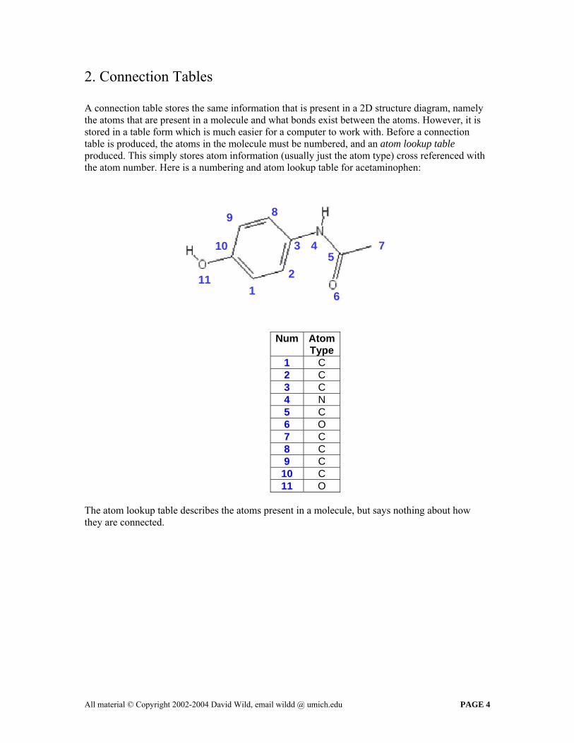
2. Connection Tables A connection table stores the same information that is present in a 2D structure diagram, namely the atoms that are present in a molecule and what bonds exist between the atoms. However, it is stored in a table form which is much easier for a computer to work with. Before a connection table is produced, the atoms in the molecule must be numbered, and an atom lookup table produced. This simply stores atom information (usually just the atom type) cross referenced with the atom number. Here is a numbering and atom lookup table for acetaminophen:

89

3 4 710 5

211 1 6

Num AtomType

1 C 2 C 3 C 4 N 5 C 6 O 7 C 8 C 9 C

10 C 11 O

The atom lookup table describes the atoms present in a molecule, but says nothing about how they are connected.


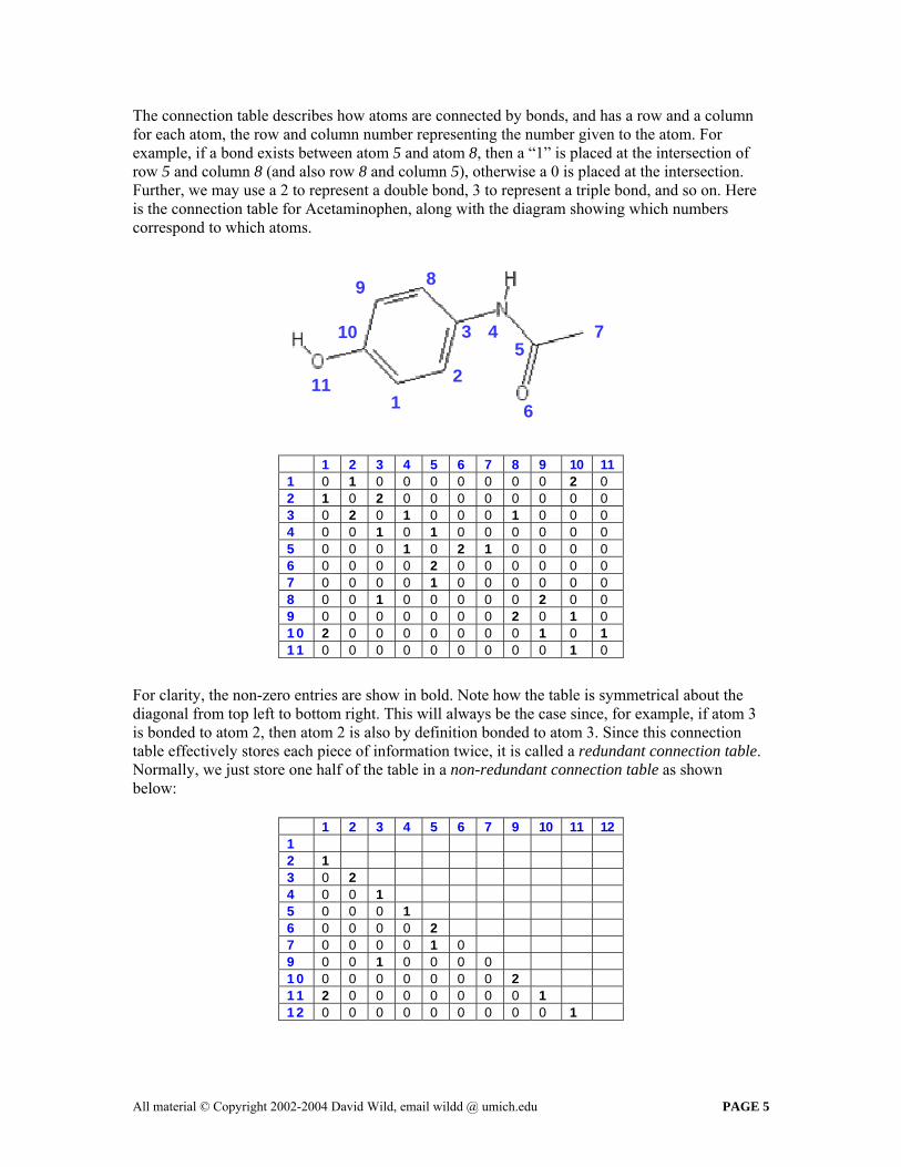
The connection table describes how atoms are connected by bonds, and has a row and a column for each atom, the row and column number representing the number given to the atom. For example, if a bond exists between atom 5 and atom 8, then a “1” is placed at the intersection of row 5 and column 8 (and also row 8 and column 5), otherwise a 0 is placed at the intersection. Further, we may use a 2 to represent a double bond, 3 to represent a triple bond, and so on. Here is the connection table for Acetaminophen, along with the diagram showing which numbers correspond to which atoms.

89

3 4 710 5

211 1 6

1 2 3 4 5 6 7 8 9 10 11 1 0 1 0 0 0 0 0 0 0 2 0 2 1 0 2 0 0 0 0 0 0 0 0 3 0 2 0 1 0 0 0 1 0 0 0 4 0 0 1 0 1 0 0 0 0 0 0 5 0 0 0 1 0 2 1 0 0 0 0 6 0 0 0 0 2 0 0 0 0 0 0 7 0 0 0 0 1 0 0 0 0 0 0 8 0 0 1 0 0 0 0 0 2 0 0 9 0 0 0 0 0 0 0 2 0 1 0 10 2 0 0 0 0 0 0 0 1 0 1 11 0 0 0 0 0 0 0 0 0 1 0

For clarity, the non-zero entries are show in bold. Note how the table is symmetrical about the diagonal from top left to bottom right. This will always be the case since, for example, if atom 3 is bonded to atom 2, then atom 2 is also by definition bonded to atom 3. Since this connection table effectively stores each piece of information twice, it is called a redundant connection table. Normally, we just store one half of the table in a non-redundant connection table as shown below:

1 2 3 4 5 6 7 9 10 11 12 1 2 1 3 0 2 4 0 0 1 5 0 0 0 1 6 0 0 0 0 2 7 0 0 0 0 1 0 9 0 0 1 0 0 0 0 10 0 0 0 0 0 0 0 2 11 2 0 0 0 0 0 0 0 1 12 0 0 0 0 0 0 0 0 0 1


3. Computer-friendly ways of storing & communicating structure Connection tables are excellent for internal computer storage, but are a little cumbersome for communicating chemical information between computers (especially since the atom numbering system also has to be communicated), and they are not really humanly readable. Therefore systems have been developed for concisely communicating chemical structures. These systems fall into two main categories: those derived directly from the connection table, and linear notations. The methods derived directly from the connection table generally consist of a list of atom records, which identify the atoms present, and then a list of bond records that specify the connectivity information. Probably the most popular of these formats is the MDL MOL File (for a specification see http://www.mdl.com/downloads/public/ctfile/ctfile.jsp). Here is a sample MOL file

Linear notations, on the other hand, attempt to condense all of the connectivity information into a single text string. The two most popular formats are SMILES (from Daylight) and SLN (Tripos format inspired by SMILES). For example, the SMILES representation of the structure in the MOL file above is:

CC(N)CC(=O)O Note that in both cases, there is an implicit hydrogen on one of the oxygens that is not explicitly represented. The SMILES format is described more thoroughly below. The great advantage of these methods is brevity – for example an entire SMILES string can be stored in a single spreadsheet cell. However, it is hard to add additional information (coordinates, properties, etc) in these formats in an elegant way. A very recent development is the Chemical Markup Language (CML), a derivative of XML. This system uses XML tags to describe chemical information, including connection table information. It has yet to find widespread use, but you can find details at http://www.xml-cml.org.


http://www.mdli.com/tech/fileformats.htm

http://www.xml-cml.org/

4. Some nuances of chemical structure representation There are some “nuances” of representing 2D structures that are not immediately obvious, but which can cause problems for computer representations. They are: Stereochemistry: Most representations don’t inherently store stereochemical information (cis- and trans- isomers, etc). Some derivative formats have been developed that do contain this information (e.g. Isomeric SMILES is a stereochemistry-aware derivative of SMILES) Aromaticity: Some scientists prefer to represent aromatic rings as Kekule structures (i.e. alternating double and single bonds), and others using aromatic notation, i.e.

Kekule Aromatic Notation

On computer, we can either represent these kinds of rings as alternating single and double bonds, or as specific aromatic bonds. Should we have a standard form and convert all structures to it? What about structures where the aromaticity isn’t clear? Do we consider these structures the same? Tautomerism: A number of groups that involve electron delocalization are difficult to define in terms of single and double bonds. For example, the Nitro group can be defined in a number of ways in a 2D structure diagram:

In some instances, we would wish to treat these as equivalent. In others, we wish to represent the fact that only one tautomeric form is possible (e.g. that an oxygen is always protonated in vivo). This ambiguity can cause problems in representation.


5. The SMILES system SMILES (standing for Simplified Molecular Input Line Entry Specification) was developed by researchers in the US government one of whom went on to create a chemoinformatics company that markets tools based upon the language and its derivatives (http://www.daylight.com). An excellent set of resources is available in the SMILES homepage on the Daylight website (http://www.daylight.com/dayhtml/smiles/index.html), including a full tutorial. Here we will just briefly cover some of the basics and give some examples. In SMILES, atoms are generally represented by their chemical symbol, with upper-case representing an aliphatic atom (C = aliphatic carbon, N = aliphatic nitrogen, etc) and lower-case representing an aromatic atom (c = aromatic carbon, etc). Hydrogens are not normally represented explicitly. Consecutive characters represent atoms bonded together with a single bond. Therefore, the SMILES for propane would simply be:

CCC Or 1-propanol would be:

CCCO Double bonds are represented by an “=” sign, e.g. propene would be

C=CC Parentheses are used to represent branching in the molecule, e.g. the SMILES for Isopropyl alcohol (2-propanol) is:

CC(O)C

Atoms other than the major organic ones (C, S, N, O, P, Cl, Br, I, B) or ions must be enclosed in square brackets. Ring enclosures are represented by using numbers to signify attachment points, usually starting at 1. The first occurrence of the number defines the attachment point, and subsequent occurrences indicate that the structure joins back to the attachment point at that position. For example, the SMILES for Benzene is as follows (note the small ‘c’ for aromatic carbon):

c1ccccc1 We can also use branching from the ring system, e.g.

c1cc(Br)ccc1 represents bromobenzene. Note that in many cases there can be several SMILES to represent the same structure – for example, we could alternatively represent bromobenzene as:

c1cccc(Br)c1

So here is a SMILES representation for acetaminophen, the structure at the top of this document:

c1c(O)ccc(NC(=O)C)c1


http://www.daylight.com/

http://www.daylight.com/dayhtml/smiles/index.html

A nice thing about SMILES is it can easily be stored in text or spreadsheet documents. For example, “SMILES files” containing SMILES, structure names or IDs, and sometimes data are often used to transfer information about structures between computers and scientists. Here is a sample of what a short SMILES file might look like: c1ccccc1 Benzene c1cc(Br)ccc1 Bromobenzene c1c(O)ccc(NC(=O)C)c1 Acetaminophen It is good to understand how SMILES works, but it is unusual for humans to have to do the job of working out SMILES. Normally conversion to and from SMILES is done by the computer using drawing and depiction tools which are described below. 6. Drawing and depicting 2D structures There are quite a few software packages available that will allow the conversion of 2D structure diagrams into computer representations (drawing tools) and the conversion of computer representations into 2D structure diagrams (depiction tools). Some are packages that must be installed on your computer, and some are available over the web. Here is a list of some of the most popular tools. You are encouraged to try out some of the web depiction and drawing tools using the structures described above. Web-based drawing tools JME (http://www.molinspiration.com/cgi-bin/properties) is a clean, simple Java drawing tool. Draw your structure and click on the smiley face to show the SMILES. This page is also a demo that will calculate some molecular properties for your structure. Marvin Sketch (http://www.chemaxon.com/marvin/sketch/demo-awt10.html) is a Java applet that allows you to draw structures, and export them as SMILES, MDL MOL files or others. Try drawing a structure, and clicking on the SMILES…..WRITE button to copy the SMILES into the box at the top, or select MDL MOLfile …. WRITE button to open a window containing the MDL MOL file. Web-based depiction tools Daylight Depiction Tool (http://www.daylight.com/daycgi/depict) is a very simple to use tool that allows you to enter a SMILES string and will then produce a 2D structure diagram from it. CACTVS GIF generator (http://www2.chemie.uni-erlangen.de/services/gifcreator/index.html) has a more complex interface, but allows many more options for producing GIF picture files of SMILES or other format structures. The quality of the images is superior to the daylight tool. Other drawing and depiction tools ChemDraw (http://www.cambridgesoft.com/products/family.cfm?FID=2) is a very popular program for sketching high-quality 2D structures that is closely integrated with Word, Powerpoint, etc. It is also able to export structures in SMILES format.


http://www.molinspiration.com/cgi-bin/properties

http://www.chemaxon.com/marvin/sketch/demo-awt10.html

http://www.daylight.com/daycgi/depict

http://www2.chemie.uni-erlangen.de/services/gifcreator/

http://www.sisweb.com/software/csw/chemoffice/chemdraw.html

MDL Chime (http://www.mdlchime.com) is a browser-based plugin that can display both 2D and interactive 3D structures in web pages. This tool will be discussed in the class on 3D representation. 7. Summary We have looked at methods for converting the information in 2D structure diagrams into more computer-friendly formats. The atom lookup and connection tables describe the atoms in a molecule and the bonds between them respectively, and are ideal for internal representation on computer. Connection-table derived and linear formats can also be used to communicate structural information between computers, and between humans and computers. The SMILES linear notation has been described in detail. Finally, some web-based and other tools have been introduced that will automate the process of generating computer-based formats from 2D structures, and 2D structure depictions from computer-based formats.


http://www.mdlchime.com/

2. REPRESENTING AND VISUALIZING 3D CHEMICAL STRUCTURES

Learning Objectives: • Know the three main sources of 3D information • Understand the coordinate table and distance matrix representations • Understand the problem of conformational flexibility, and be able to list three ways

of dealing with it • Be able to give the names of 3 structure generation programs • Understand the term “minimized structure” • Be able to use web-based Corina service to generate a 3D structure from a 2D one • Be able to use the DS ViewerLite program to load, rotate and zoom a 3D structure,

and add a volume surface to it. 1. Introduction Whilst 2D representations describe the connectivity of the atoms in molecule, 3D representations describe how the molecule is arranged in three-dimensional space. Thus it is believed that 3D representations are closer to how the molecule really exists than two-dimensional representations. This makes 3D representations particularly useful for such applications as computation of molecular properties, visualization and prediction of how molecules bind to proteins. We will cover such applications in class 8. 3D information can be obtained through X-ray crystallography, NMR spectroscopy or by computational means. The basic forms of 3D representation are the coordinate table and the distance matrix. The coordinate table also forms the basis of 3D molecule file formats. One major issue in 3D representation is that rotatable bonds are present in most molecules, and thus the molecule is flexible. Handling of this conformational flexibility is also described. Next, ways of computationally deriving 3D information are described. Finally, tools for the depiction of 3D structures are illustrated.


2. Sources of 3D information The two ways of experimentally obtaining a 3D structure are X-ray crystallography and NMR spectroscopy. Both of these methods can be used to obtain structures for small molecules and proteins. X-ray crystallography exploits the fact that concentrations of electrons (e.g. around atoms) cause x-rays to be diffracted. When a crystalline sample is used, this effect is amplified so that the positions of the atoms in 3D space can be determined. For more information, see http://www-structure.llnl.gov/Xray/101index.html NMR spectroscopy exploits the magnetic fields created by quantum spin in atomic nuclei. When radio waves are applied, the quantum spin can switch state at a resonant frequency which is dependent on the atoms and functional groups. A plotting procedure can then be used to coalesce this information into a 3D structure. For more information, see http://www.rod.beavon.clara.net/nmr1.htm Finally, 3D structures can be generated by computer programs. Three of these are discussed below.


http://www-structure.llnl.gov/Xray/101index.html

http://www-structure.llnl.gov/Xray/101index.html

http://www.rod.beavon.clara.net/nmr1.htm

3. Coordinate Tables and Distance Matrices A coordinate table is simply an extension of the atom lookup table that also contains coordinates for each atom. These coordinates are relative to a consistent origin. Here is a sample coordinate table for Aspirin, along with a 3D structure with the atoms numbered:

Atom Label X Y Z

1 C -1.8920 -0.9920 -1.5760

2 C -1.3680 -2.1480 -0.9880

3 C -0.0760 -2.1440 -0.4640

4 C 0.7080 -0.9840 -0.5200

5 C 0.2000 -0.1560 -1.1960

6 C -0.1080 0.1600 -1.6520

7 O 2.0840 -1.0280 0.1040

8 O 2.5320 -2.0320 0.6360

9 C 2.8760 0.0240 0.1120

10 O 0.7520 1.3320 -1.0840

11 O 0.6680 2.0240 0.0320

12 C 1.3000 3.0600 0.1520

13 C -0.2400 1.5760 1.4440

2

3 1

11

4 12

9 5

10 13 6

7 8

Distance matrices are similar to connection tables (see 2D class notes), except that instead of storing connectivity information, they store relative distances (in Ångström) between all atoms. Here is a sample distance matrix for the Aspirin molecule above:

1 2 3 4 5 6 7 8 9 10 11 12 13

1 1.4 2.4 2.8 2.4 3.8 4.8 4.2 1.4 2.4 2.7 2.9 4.3

2 1.4 2.4 2.8 4.3 5.1 5.0 2.4 3.7 3.9 4.2 5.6

3 1.4 2.4 3.8 4.2 4.8 2.8 4.2 4.7 4.9 6.4

4 1.4 2.5 2.8 3.6 2.4 3.7 4.7 4.6 6.1

5 1.5 2.4 2.3 1.4 2.3 3.7 3.5 4.8

6 1.3 1.2 2.5 2.8 4.4 3.9 5.0

7 2.2 3.7 4.1 5.7 5.2 6.3

8 2.8 2.5 4.2 3.5 4.3

9 1.4 2.6 2.3 3.7

10 2.2 1.3 2.5

11 1.2 2.4

12 1.5

13

Distance matrices are useful when comparing molecules with each other, whereas coordinate tables tend to be used for structure visualization. Note that it is easy to create a distance matrix from a coordinate table, but harder to go the other way.


4. 3D file formats

3D file formats are generally contain both coordinate / atom lookup table information and connection table information. The two main formats are the MDL MOL file (same as the 2D one but with coordinates added) and the SYBYL MOL2 format. Here is a sample MDL 3D MOL file for Aspirin. Chime 12290214053D 21 21 0 0 1 V2000 -1.8920 -0.9920 -1.5760 C 0 0 0 0 0 0 0 0 0 0 0 0 -1.3680 -2.1480 -0.9880 C 0 0 0 0 0 0 0 0 0 0 0 0 -0.0760 -2.1440 -0.4640 C 0 0 0 0 0 0 0 0 0 0 0 0 0.7080 -0.9840 -0.5200 C 0 0 0 0 0 0 0 0 0 0 0 0 0.2000 0.1560 -1.1960 C 0 0 0 0 0 0 0 0 0 0 0 0 -1.1080 0.1600 -1.6520 C 0 0 0 0 0 0 0 0 0 0 0 0 2.0840 -1.0280 0.1040 C 0 0 0 0 0 0 0 0 0 0 0 0 2.5320 -2.0320 0.6360 O 0 0 0 0 0 0 0 0 0 0 0 0 2.8760 0.0240 0.1120 O 0 0 0 0 0 0 0 0 0 0 0 0 0.7520 1.3320 -1.0840 O 0 0 0 0 0 0 0 0 0 0 0 0 0.6680 2.0240 0.0320 C 0 0 0 0 0 0 0 0 0 0 0 0 1.3000 3.0600 0.1520 O 0 0 0 0 0 0 0 0 0 0 0 0 -0.2400 1.5760 1.1440 C 0 0 0 0 0 0 0 0 0 0 0 0 -2.8760 -0.9600 -1.9840 H 0 0 0 0 0 0 0 0 0 0 0 0 -1.9880 -3.0360 -0.9520 H 0 0 0 0 0 0 0 0 0 0 0 0 0.3000 -3.0600 -0.0040 H 0 0 0 0 0 0 0 0 0 0 0 0 -1.4880 1.0840 -2.0560 H 0 0 0 0 0 0 0 0 0 0 0 0 2.5640 0.7800 -0.3240 H 0 0 0 0 0 0 0 0 0 0 0 0 -0.7600 0.6360 0.9320 H 0 0 0 0 0 0 0 0 0 0 0 0 -1.0080 2.3480 1.2880 H 0 0 0 0 0 0 0 0 0 0 0 0 0.3440 1.4320 2.0560 H 0 0 0 0 0 0 0 0 0 0 0 0 13 21 1 0 13 20 1 0 13 19 1 0 11 13 1 0 11 12 1 0 10 11 1 0 9 18 1 0 7 9 1 0 7 8 1 0 6 17 1 0 5 10 1 0 5 6 1 0 4 7 1 0 4 5 1 0 3 16 1 0 3 4 1 0 2 15 1 0 2 3 1 0 1 14 1 0 1 6 1 0 1 2 1 0 M END


5. Rotatable bonds and conformational flexibility Most compounds have rotatable or movable bonds, meaning that the molecule can take on many 3D conformations. A rotatable bond may be defined as any single bond which is not in a ring, terminal, or part of a ring system. The amount of rotation of a rotatable bond is measured using the torsion (τ) angle (also known as the dihedral angle).This is defined as the relative position, or angle, between the A-B bonds and the C-D bonds when considering four atoms connected in the order A-B-C-D:

Other forms of conformation change are possible, e.g. a cyclohexane ring can take chair or boat conformations:

Molecules prefer low-energy states, so low-energy conformations are more likely. There are three approaches to handling conformational flexibility:

1. Use just a single conformation (either a computationally-minimized structure or one derived from X-ray/NMR)

2. Pick multiple low energy structures that represent the most likely conformations in the environment of interest and treat each as a separate structure

3. Use representations and algorithms that incorporate flexibility The approach used will depend on the application.

Chair Boat

C

A

B C

D A D

B

ττ


6. Structure generation and minimization Several computational tools are available for generating 3D structures from input files of 2D structures. Three of the most popular are: Concord from Tripos, Inc. This was one of the first 3D structure generation programs, and is still being refined and developed by Tripos. The program generates single, minimal-energy structures from input 2D structures. The program can input and output a variety of file formats. More information is available at http://www.tripos.com/sciTech/inSilicoDisc/chemInfo/concord.html Corina from the Gasteiger group. This program is similar in function to Concord. It is made available on the web for anyone to try out (with a limit of 1,000 structures per user) at: http://www2.chemie.uni-erlangen.de/software/corina/free_struct.html Omega from OpenEye is the latest release. It offers very fast generation of multiple low-energy conformers. An academic-use license may be obtained at no cost for academic projects. More information from http://www.eyesopen.com/omega/ These programs generally do some form of minimization (or minimization may be performed after structure generation). Minimization involves finding the conformation or conformations that have the lowest energy, and are therefore most likely to be found in nature. This kind of conformational search may start with an existing non-optimized structure, and can use standard optimization methods such as exhaustive search, simulated annealing, monte carlo, or genentic algorithms. The optimization methods generally try to optimize based on force-field equations. For more information see: http://www.chem.swin.edu.au/modules/mod6/ 7. Other kinds of 3D information Other forms of 3D information may be stored, such as:

• Surface (van de Waal’s, Connolly, volume) • Properties projected onto surface (electrostatics, hydrophobics) • Fields (energy, force, electrostatic, steric, hydrophobic) • Atom-based properties (charge, hydrophobicity, etc)

These will not be covered in great detail in this course.


http://www.tripos.com/sciTech/inSilicoDisc/chemInfo/concord.html

http://www2.chemie.uni-erlangen.de/software/corina/free_struct.html

http://www.eyesopen.com/omega/

http://www.chem.swin.edu.au/modules/mod6/

8. Depiction Tools for 3D structures Two tools are recommended for use in this course. MDL Chime is a web browser plug-in that allows 2D and 3D structures to be viewed in web pages. It can be used to visualize both proteins and small molecules, and includes some limited ability to create molecular surfaces. It is excellent for communicating structures via the web and for use in writing web-based chemoinformatics software.

Demonstrations of Chime are available on the web, at http://www.wild-ideas.org/moldemos, or you can download the Chime plug-in at http://www.mdl.com/chime/index.html. Accelrys DS ViewerLite (formerly called Web Lab Viewer) was a free, standalone 3D visualization program for Windows from Accelrys. It has excellent facilities for visualizing small molecules and/or proteins and can produce good quality images for pasting into Word, Powerpoint, etc. Limited molecular modeling features are also available (rotate bonds, delete or amend atoms). Unfortunately, the free copy is no longer available, but a trial of the professional version is available at: http://www.accelrys.com/dstudio/ds_viewer/register/lite/viewerlite_reg.php


http://www.wild-ideas.org/moldemos

http://www.mdl.com/chime/index.html

http://www.accelrys.com/dstudio/ds_viewer/register/lite/viewerlite_reg.php

ViewerLite usage hints: 1. Turn on hardware graphics acceleration (View -> Options -> General tab -> uncheck

“Disable graphics hardware acceleration”) 2. Disable fast render on move (View -> Options -> Graphics tab -> uncheck “Fast render on

move”)


3. REPRESENTING AND VISUALIZING MACROMOLECULES

Learning Objectives: • Understand the basic structure of proteins • Understand the meaning of Atomic, Primary, Secondary, and Tertriary information • Know how these forms of information are stored on computer • Be able to understand a PDB file by inspection • Name three methods used to help prediction of tertiary structure • Know the two common kinds of protein surface • Be able to use the DS ViewerLite program to load, rotate and zoom a protein/drug

complex, visualize with ribbon and tube depiction, and add a volume surface to it.

1. Introduction Macromolecules is a term used to describe large molecules, containing thousands of atoms. Common examples are proteins, peptide sequences, nucleotide sequences, and polysaccharides. Macromolecules are generally made up of a sequence of building blocks: proteins are made from chains of amino acids; nucleotides are made from chains of bases; polysaccharides are chains of sugars, and so on. These properties, along with the sheer size of macromolecules, mean that special techniques are used to handle and represent them. This material will focus on proteins. In living organisms, proteins are formed from single or multiple chains of amino acids. Each amino acid is connected to the next by means of a peptide bond. 2. Types of protein information Four types of information are considered here: atomic, primary structure (sequence), secondary structure and tertiary structure. Atomic information Atomic information is simply standard 3D coordinate information (as used to represent small molecules – see last class) applied to a protein structure. The information is stored in the standard way (coordinate table, distance matrix). Atomic information is gained using exactly the same experimental techniques as for small structures – X-ray crystallography and NMR spectroscopy. Primary structure (sequence) information The primary structure, also known as the sequence, is a list of the amino acids present in a protein chain, in the order that they are bound together in the chain. The primary structure may be given as a list of standard three-letter abbreviations, e.g.:

Ser-Tyr-Ser-Met-Glu-His-Phe-Arg-Trp-Gly-Lys


Alternatively, the standard single letter abbreviations may be used:

S Y S M E H F R W G K This kind of “1-dimensional” information can clearly be stored computationally as a text string. Secondary structure information Certain chains of amino acid sequences have a tendency to form themselves into particular 3D forms. These forms include alpha-helices which are formed by hydrogen-bonding between the C=O and NH groups on amino acids four places apart in the chain. Beta sheets are also formed by hydrogen bonding, this time between parts of the chain, forming a flat structure. Turns are twisted structures that cause the chain to change direction.

α-helix β-sheet It is possible to predict which areas of a primary structure are likely to form secondary structural elements, and this is especially easy if coordinate information is available. Secondary structural information can be stored computationally simply by “tagging” amino acids to indicate which kind of secondary structure (if any) they are in. For example,

G A F T G E I S P G M I K D C G A T W V β β β β β β β α α α α α α α

Tertiary structure information Proteins are made of long, flexible chains of amino acids, and these chains can ‘fold’ up in many ways. However, individual proteins will generally always take on the same ‘folding’, which is believed to be a product of their sequence, electrostatic and hydrophobic properties, and the action of chaperone proteins during formation. The tertiary structure describes how a protein is folded up in three-dimensions, and thus shows the overall shape of the protein. The tertiary structure is usually derived from coordinate information, since it is extremely difficult to predict from primary or secondary structure. However, techniques such as secondary structure prediction, homology modeling and threading, described later, can help in this process. Tertiary structure can be represented on computer using just the atomic coordinates, or as a series of points and vectors. Here is an example visualization of HIV-1 Protease, showing secondary and tertiary structural information. The main protein chain folding is shown as a thin tube, with beta sheets shown in blue, alpha helices in red, and turns in green.


3. Protein/macromolecule file formats The most popular file format for proteins is the PDB file, which is specifically designed for proteins and can hold all the different kinds of protein information. Tripos Sybyl MOL2 files are also used for storing atom information for proteins. PDB file format The PDB-file is split into a number of (optional) sections, each of which pertains to a particular kind of information. The sections are: title, primary structure, heterogen, secondary structure, connectivity annotation, miscellaneous, coordinate, connectivity and book-keeping. Each section contains keywords (one per line) which detail a particular piece of information. Some of the more important sections are described below. For a complete reference, see the official PDB file format guide at http://www.rcsb.org/pdb/docs/format/pdbguide2.2/guide2.2_frame.html. The title section is used to describe general title, comment, etc. information about the protein stored in the file. Common keywords are: HEADER (type, date, ID code), COMPND (name of protein), TITLE (title of experiment used to create the file), AUTHOR, JRNL (reference journal article) and REMARK. The primary structure section lists the primary sequence, mainly through the SEQRES keyword. The secondary structure tags secondary structural features with the HELIX, SHEET, and TURN keywords, identifying starting and ending amino acids for a feature. The coordinates section gives atomic coordinates for all atoms (i.e. a coordinate table), with the ATOM and HETATM keywords for amino-acid and non amino-acid residues respectively. Finally, the connectivity section provides a connection table through the CONECT keyword, mainly for non amino-acid parts of the structure (since amino-acid connectivity is already known). Here is an example PDB file for HIV-1 Protease, with some parts omitted for brevity. This file contains title, primary structure, coordinate and connectivity sections, as well as a mandatory book-keeping section. HEADER PROTEIN 28-OCT-96 COMPND HIV-1 PROTEASE COMPLEXED WITH THE INHIBITOR A77003 (R,S) AUTHOR GENERATED BY SYBYL, A PRODUCT OF TRIPOS ASSOCIATES, INC. SEQRES 1 A 99 PRO GLN ILE THR LEU TRP GLN ARG PRO LEU VAL THR ILE SEQRES 2 A 99 LYS ILE GLY GLY GLN LEU LYS GLU ALA LEU LEU ASP THR SEQRES 3 A 99 GLY ALA ASP ASP THR VAL LEU GLU GLU MET SER LEU PRO SEQRES 4 A 99 GLY ARG TRP LYS PRO LYS MET ILE GLY GLY ILE GLY GLY SEQRES 5 A 99 PHE ILE LYS VAL ARG GLN TYR ASP GLN ILE LEU ILE GLU SEQRES 6 A 99 ILE CYS GLY HIS LYS ALA ILE GLY THR VAL LEU VAL GLY SEQRES 7 A 99 PRO THR PRO VAL ASN ILE ILE GLY ARG ASN LEU LEU THR SEQRES 8 A 99 GLN ILE GLY CYS THR LEU ASN PHE SEQRES 1 B 99 PRO GLN ILE THR LEU TRP GLN ARG PRO LEU VAL THR ILE SEQRES 2 B 99 LYS ILE GLY GLY GLN LEU LYS GLU ALA LEU LEU ASP THR SEQRES 3 B 99 GLY ALA ASP ASP THR VAL LEU GLU GLU MET SER LEU PRO SEQRES 4 B 99 GLY ARG TRP LYS PRO LYS MET ILE GLY GLY ILE GLY GLY SEQRES 5 B 99 PHE ILE LYS VAL ARG GLN TYR ASP GLN ILE LEU ILE GLU SEQRES 6 B 99 ILE CYS GLY HIS LYS ALA ILE GLY THR VAL LEU VAL GLY SEQRES 7 B 99 PRO THR PRO VAL ASN ILE ILE GLY ARG ASN LEU LEU THR SEQRES 8 B 99 GLN ILE GLY CYS THR LEU ASN PHE ATOM 1 N PRO A 1 8.133 -13.258 12.706 1.00 0.00 ATOM 2 CA PRO A 1 9.325 -12.418 13.001 1.00 0.00 ATOM 3 C PRO A 1 8.939 -10.978 13.283 1.00 0.00 ATOM 4 O PRO A 1 7.813 -10.607 13.030 1.00 0.00 ATOM 5 CB PRO A 1 10.211 -12.484 11.768 1.00 0.00 ATOM 6 CG PRO A 1 9.219 -12.779 10.674 1.00 0.00 ATOM 7 CD PRO A 1 8.271 -13.768 11.335 1.00 0.00 ATOM 8 H1 PRO A 1 7.974 -14.024 13.392 1.00 0.00


http://www.rcsb.org/pdb/docs/format/pdbguide2.2/guide2.2_frame.html

(region omitted here for brevity) ATOM 1844 CE2 PHE B 99 5.527 -13.746 8.735 1.00 0.00 ATOM 1845 CZ PHE B 99 6.308 -12.665 8.239 1.00 0.00 ATOM 1846 OXT PHE B 99 5.672 -12.903 13.426 1.00 0.00 ATOM 1847 H PHE B 99 5.668 -10.590 12.626 1.00 0.00 TER 1848 PHE B 99 HETATM 1849 C1 A 1 -3.676 0.038 -4.301 1.00 0.00 HETATM 1850 N21 A 1 -2.730 -0.070 -5.222 1.00 0.00 HETATM 1851 H28 A 1 -2.958 0.299 -6.126 1.00 0.00 HETATM 1852 C22 A 1 -1.389 -0.623 -4.962 1.00 0.00 HETATM 1853 H29 A 1 -1.369 -1.096 -3.981 1.00 0.00 HETATM 1854 C25 A 1 -1.031 -1.707 -6.000 1.00 0.00 HETATM 1855 H30 A 1 -1.021 -1.235 -6.985 1.00 0.00 HETATM 1856 C27 A 1 -2.085 -2.821 -6.044 1.00 0.00 HETATM 1857 H36 A 1 -1.845 -3.547 -6.818 1.00 0.00 HETATM 1858 H35 A 1 -3.079 -2.429 -6.267 1.00 0.00 HETATM 1859 H34 A 1 -2.140 -3.350 -5.091 1.00 0.00 HETATM 1860 C26 A 1 0.365 -2.310 -5.758 1.00 0.00 HETATM 1861 H33 A 1 0.450 -2.709 -4.748 1.00 0.00 HETATM 1862 H32 A 1 1.159 -1.573 -5.891 1.00 0.00 HETATM 1863 H31 A 1 0.564 -3.134 -6.440 1.00 0.00 HETATM 1864 C23 A 1 -0.360 0.506 -4.927 1.00 0.00 HETATM 1865 N37 A 1 -0.195 1.091 -3.733 1.00 0.00 HETATM 1866 H59 A 1 -0.715 0.711 -2.967 1.00 0.00 HETATM 1867 C38 A 1 0.602 2.329 -3.511 1.00 0.00 HETATM 1868 H60 A 1 1.052 2.671 -4.449 1.00 0.00 HETATM 1869 C46 A 1 1.713 2.066 -2.491 1.00 0.00 HETATM 1870 H68 A 1 1.221 1.950 -1.522 1.00 0.00 (region omitted here for brevity) CONECT 1943 1934 1941 1944 CONECT 1944 1943 CONECT 1945 1864 CONECT 1946 1849 1947 1960 CONECT 1947 1946 1948 1949 1950 CONECT 1948 1947 CONECT 1949 1947 CONECT 1950 1947 1951 1958 CONECT 1951 1950 1952 CONECT 1952 1951 1953 1954 CONECT 1953 1952 CONECT 1954 1952 1955 1956 CONECT 1955 1954 CONECT 1956 1954 1957 1958 CONECT 1957 1956 CONECT 1958 1950 1956 1959 CONECT 1959 1958 CONECT 1960 1946 1961 1962 1963 CONECT 1961 1960 CONECT 1962 1960 CONECT 1963 1960 CONECT 1964 1849 MASTER 0 0 0 0 0 0 0 0 1965 2 126 16 END


4. Prediction of tertiary structure The tertiary structure of a protein is a result of a complex set of interactions as a protein is formed, and it is thus very difficult to devise a method to predict tertiary structure directly from the sequence. However, such a method would be invaluable, especially for membrane-bound proteins, for which X-ray/NMR cannot be used. Prediction of tertiary structure (or “folding”) is currently a hot topic in structural bioinformatics. There are three ways of making the problem easier: secondary structure prediction, homology modeling and threading:

• Secondary structure prediction is much easier than prediction of tertiary structure, and knowing the secondary structural elements sets bounds on how the protein can fold.

• Homology modeling involves searching databases to find proteins from the same or

similar protein families (homologs) for which the tertiary structure is known, and then using that information to help make informed guesses as to the structure of the unknown protein. Searching may also be done for proteins with a similar primary sequence (but which may not be technically homologs).

• Threading involves maintaining databases of sequence segments and their three-

dimensional characteristics, and then attempting to “thread” the protein sequence into these segments.

There is a lot of research going on into this field, and a lot of information on the internet. Good places for introductory information are: SDSC (http://www.sdsc.edu/pb/edu/pharm207/9/9.html), the Biophysics text book (http://www.biophysics.org/btol/seq_introduction.html), and EMBL (http://speedy.embl-heidelberg.de/gtsp/). There are a number of online servers that will allow you to enter a sequence, and will attempt to predict a tertiary structure (and send the results to you be email). Two examples are: BioInBGU (http://www.cs.bgu.ac.il/~bioinbgu/) and 123D+ (http://123d.ncifcrf.gov/123D+.html).


http://www.sdsc.edu/pb/edu/pharm207/9/9.html

http://www.biophysics.org/btol/seq_introduction.html

http://speedy.embl-heidelberg.de/gtsp/

http://www.cs.bgu.ac.il/~bioinbgu/

http://123d.ncifcrf.gov/123D+.html

5. Protein visualization and surfaces Visualization methods The main tool we shall be using to demonstrate protein visualization is Accelrys DS ViewerLite, available from http://www.accelrys.com/dstudio/ds_viewer/register/lite/viewerlite_reg.php. This is a standalone program that will need to be installed on your computer. MDL Chime is also used for visualizing protein structures on the web. For more information, see http://www.mdl.com/chime/index.html. There are a number of ways of visualizing proteins in 3D. Firstly, an atom & bond view shows the atoms and bonds connecting them, just like viewing a small molecule. This kind of view can be useful when examining parts of the protein, or a protein / ligand (bound compound) interface, but tends to be overwhelming when viewing large sections of the protein. Ribbons and tubes are a reduced view which follow the backbone of the protein chain, and thus can be used to show the tertiary structure. They may also be colored to illustrate properties, such as secondary structure type and hydrophobicity. An enhanced form of this view (often called a schematic or cartoon view) highlights secondary structural elements. The images below illustrate these kinds of visualization for HIV-1 Protease

Atom & Bond View Ribbon View

Tube View Schematic View


http://www.accelrys.com/dstudio/ds_viewer/register/lite/viewerlite_reg.php

http://www.mdl.com/chime/index.html

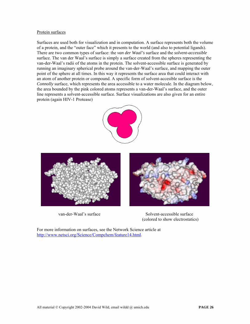
Protein surfaces Surfaces are used both for visualization and in computation. A surface represents both the volume of a protein, and the “outer face” which it presents to the world (and also to potential ligands). There are two common types of surface: the van der Waal’s surface and the solvent-accessible surface. The van der Waal’s surface is simply a surface created from the spheres representing the van-der-Waal’s radii of the atoms in the protein. The solvent-accessible surface is generated by running an imaginary spherical probe around the van-der-Waal’s surface, and mapping the outer point of the sphere at all times. In this way it represents the surface area that could interact with an atom of another protein or compound. A specific form of solvent-accesible surface is the Connolly surface, which represents the area accessible to a water molecule. In the diagram below, the area bounded by the pink colored atoms represents a van-der-Waal’s surface, and the outer line represents a solvent-accessible surface. Surface visualizations are also given for an entire protein (again HIV-1 Protease)

van-der-Waal’s surface Solvent-accessible surface (colored to show electrostatics)

For more information on surfaces, see the Network Science article at http://www.netsci.org/Science/Compchem/feature14.html.


http://www.netsci.org/Science/Compchem/feature14.html

4. SEARCHING DATABASES OF CHEMICAL STRUCTURES

Learning Objectives: • Know the three kinds of 2D searching, and the purposes for which they are used • Be able to formulate a simple SMARTS query • Understand the 2D fingerprint representation and how it is used in conjunction with

similarity coefficients • Know the formula for the Euclidean and Tanimoto coefficients • Understand how cartridges allow 2D searching in Oracle SQL statements • Understand the term “pharmacophore” and how it relates to 3D searching • Know the various methods for 3D similarity searching • Understand some strengths and weaknesses of 2D and 3D searching RECOMMENDED COMPANION READING:

Chemical Similarity Searching, P. Willett, J.M. Barnard, G.M. Downs, Journal of Chemical Information and Computer Sciences, 1998, 38, 983-99. Available at http://pubs3.acs.org/acs/journals/doilookup?in_doi=10.1021/ci9800211

1. Introduction The previous three classes have discussed the representation of 2D small molecules, 3D small molecules and proteins on computer. In this class, we shall look at how databases of structures in 2D and 3D are stored, and the kinds of searching which may be performed on them. Of particular interest are structure, substructure and similarity searching, and one of the most flexible ways of performing these searches is using Oracle Chemistry Cartridges. 3D searches are different in nature, and less well used, but can be very useful for certain applications.


http://pubs3.acs.org/acs/journals/doilookup?in_doi=10.1021/ci9800211

2. Kinds of chemistry databases • Small-molecule databases

– Databases of commercially-available compounds (e.g. ACD) – Proprietary chemical structure databases – Literature databases – Patent databases – Small project-specific databases

• Protein databases

– Public, online databases (e.g. PDB) – Proprietary and project-specific databases

3. Methods for 2D searching 2D databases are much more common than 3D databases, which are generally smaller and project-specific. 2D databases store the structural information in connection and atom-lookup tables as described in Class 2. Searching these databases based on chemical structure requires special methods, which may be found in specially written chemistry database searching programs (such as ISIS/Base from MDL or Merlin/Thor from Daylight) or, with increasing popularity using Oracle Chemistry cartridges, which allow 2D structures to be stored and searched in standard Oracle databases. There are three special kinds of chemical information searching: the structure search, substructure search and the similarity search. Structure searching This involves searching a database for an exact match with a specified query structure. Fro example, if the following is the query

Then only an exact match to this structure would be returned by a search. The techniques used to perform the search won’t be covered here, but basically they involve treating the 2D connection table as a mathematical graph, where the nodes represent atoms and the edges represent bonds, and then a test for exact match can be done using a graph isomorphism algorithm (a standard computer science technique).


http://www.mdl.com/products/acd.html

http://www.pdb.org/

Substructure searching A substructure search involves finding all the structures in a database that contain one or more particular structural fragments. For example, we might want to find all of the structures in a database which contain the nitro group:

Substructure searching requires some method of specifying a query (i.e., we want to find this and that, but not this, etc). One popular example is SMARTS, an extension to SMILES, which is described below. Mathematically, substructure searching is performed, as with structure searching, using a graph representation, but this time a subgraph isomorphism algorithm finds occurrences of subgraphs (i.e. substructures) in a structure. Similarity searching Similarity searching involves looking for all the structures in a database that are highly similar to a given structure. The most common use is to find compounds that could exhibit similar properties (based on the similar property principle that compounds with similar structures are likely to exhibit similar biological behaviors). Note that “similarity” is a subjective thing. As an example, a similarity search might involve looking for structures with a similarity greater than 0.7 to this molecule

Obviously some method is required for measuring similarity. This is usually done using fingerprint representations and similarity coefficients as described below. Note that these methods may also be used in other applications that involve measurement of similarity, for example cluster analysis. Reaction-based databases Searching databases of reactions is a little different to straight searching, although the kinds of search are the same (structure, substructure, similarity). However, searching may be done on reactants, products, or both, and searches may be performed for entire reactions (as opposed to single structures). Representation of reactions is by the usual means (connection tables, atom lookup tables), but with additional information about which molecules are products and reagents, and which reagent atoms map to which product atoms. A derivative of SMILES, called Reaction SMILES is available for representing reactions, along with a way for defining reaction queries called SMIRKS (see http://www.daylight.com/meetings/summerschool01/course/basics/smirks.html)


http://www.daylight.com/meetings/summerschool01/course/basics/smirks.html

4. SMARTS representation of 2D queries SMARTS is a superset of SMILES that is extended to allow the representation of partial structures (substructures) and queries (molecules with optional parts). One of it’s major functions is in describing queries for substructure searches. More information on SMARTS can be found on the Daylight website (at http://www.daylight.com/meetings/summerschool01/course/basics/smarts.html and http://www.daylight.com/dayhtml/doc/theory/theory.smarts.html) A very simple SMARTS would be:

*C(=O)O where the * is a special character which represents any atom (i.e. an attachment point in this case). Thus this SMARTS would represent a query for a carboxylic acid:

Actually, there are many special characters which are used in SMARTS. Here are some of them:

* Any atom ~ Any bond

a Aromatic atom : Aromatic bond

A Aliphatic atom @ Any ring bond

R Ring atom & Logical AND

Rn Atom in ring of size n ; Logical AND (low prec.)

Hn n attached hydrogens , Logical OR

Xn n total connections ! Logical NOT

and here are some sample SMARTS which use the characters, along with the meaning of the SMARTS:

[!C;R] Any atom in a ring that is not aliphatic Carbon

[O;H1] Hydroxyl group (-OH)

c:c Two carbons separated by aromatic bond

C~N Carbon and nitrogen attached by any bond

*C(=O)O Carboxyl Group


http://www.daylight.com/meetings/summerschool01/course/basics/smarts.html

http://www.daylight.com/dayhtml/doc/theory/theory.smarts.html

Thus we could perform a SMARTS search for all molecules that contain a carboxyl group and an aromatic nitrogen in a ring with the following query:

[!C;R]&*C(=O)O

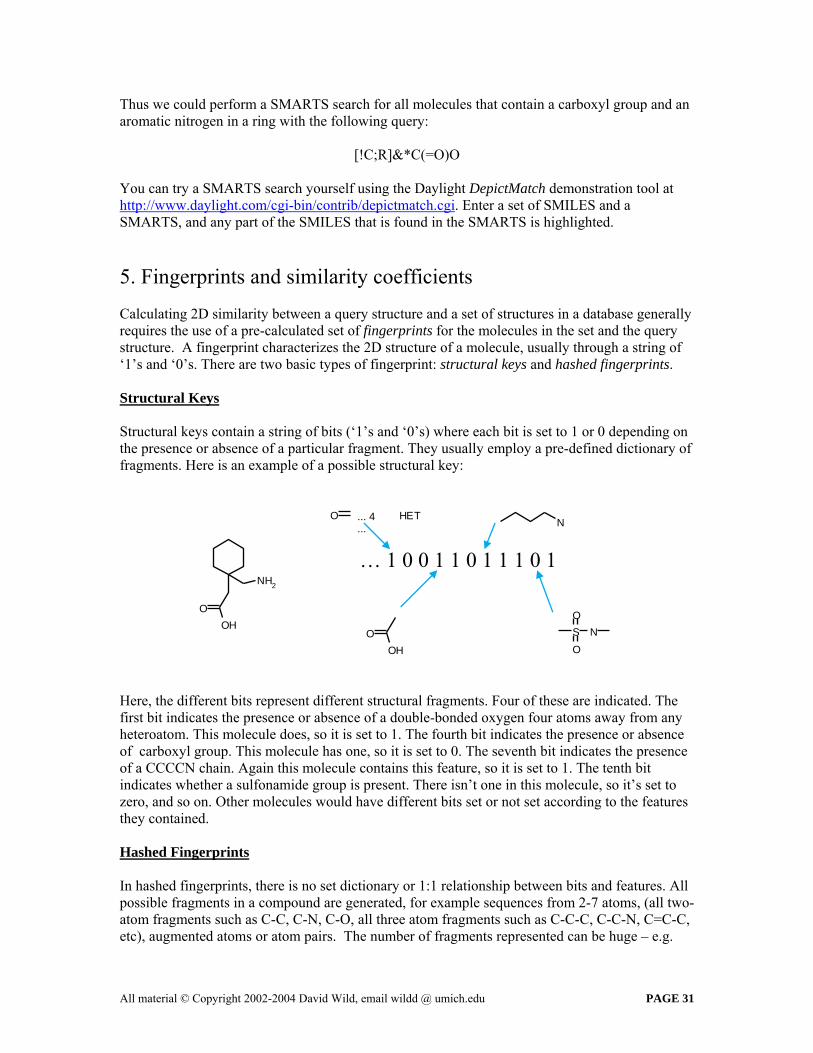
You can try a SMARTS search yourself using the Daylight DepictMatch demonstration tool at http://www.daylight.com/cgi-bin/contrib/depictmatch.cgi. Enter a set of SMILES and a SMARTS, and any part of the SMILES that is found in the SMARTS is highlighted. 5. Fingerprints and similarity coefficients Calculating 2D similarity between a query structure and a set of structures in a database generally requires the use of a pre-calculated set of fingerprints for the molecules in the set and the query structure. A fingerprint characterizes the 2D structure of a molecule, usually through a string of ‘1’s and ‘0’s. There are two basic types of fingerprint: structural keys and hashed fingerprints. Structural Keys Structural keys contain a string of bits (‘1’s and ‘0’s) where each bit is set to 1 or 0 depending on the presence or absence of a particular fragment. They usually employ a pre-defined dictionary of fragments. Here is an example of a possible structural key:

O

Here, the different bits represent different structural fragments. Four of these are indicated. The first bit indicates the presence or absence of a double-bonded oxygen four atoms away from any heteroatom. This molecule does, so it is set to 1. The fourth bit indicates the presence or absence of carboxyl group. This molecule has one, so it is set to 0. The seventh bit indicates the presence of a CCCCN chain. Again this molecule contains this feature, so it is set to 1. The tenth bit indicates whether a sulfonamide group is present. There isn’t one in this molecule, so it’s set to zero, and so on. Other molecules would have different bits set or not set according to the features they contained. Hashed Fingerprints In hashed fingerprints, there is no set dictionary or 1:1 relationship between bits and features. All possible fragments in a compound are generated, for example sequences from 2-7 atoms, (all two-atom fragments such as C-C, C-N, C-O, all three atom fragments such as C-C-C, C-C-N, C=C-C, etc), augmented atoms or atom pairs. The number of fragments represented can be huge – e.g.

O O H

N H 2 … 1 0 0 1 1 0 1 1 1 0 1

OOH

HE N... 4 ...

T

O S N O


http://www.daylight.com/cgi-bin/contrib/depictmatch.cgi

100,000 for just the 2-7-length sequences for C, N, S, O, P, not considering bond types or generalizations. Thus rather than assigning one bit position for each fragment, the bits are “hashed” down onto a fixed number of bits (e.g. 1024). Thus hashed fingerprints are a less precise form, but they carry more information. Fingerprint generation packages A number of companies market fingerprint generation packages, which rapidly create fingerprints for molecules. Some common examples are: Daylight Fingerprints (hashed - see http://www.daylight.com/dayhtml/doc/theory/theory.finger.html); Tripos Unity Fingerprints (hybrid), MDL MACCS Keys (166 structural keys) and BCI Fingerprints (hybrid - see http://www.bci.gb.com/products/fingerprints.htm). Measuring similarity using fingerprint representations Once fingerprint representations are available, similarity coefficients can be used to give a measure of similarity between two fingerprints. Two of the most common are the Tanimoto coefficient (also known as the Jaccard coefficient) and Euclidean distance (actually a distance calculation, but it can be inverted for similarity). The Tanimoto coefficient effectively measures the number of ‘1’s in common as a fraction of the total number of ‘1’s that are different. The Tanimoto similarity between two fingerprints a and b is defined as:

c Tanimoto similarity = ------------------

#a + #b - c where c is the number of ‘1’s in common between the two bitstrings, #a is the total number of ‘1’s set in a, and #b is the total number of ‘1’s in b. The similarity will always be between 0 (no similarity) and 1 (exact match). Here is an example:

a 101101011 b 011101101

here, a is 6, since there are six ‘1’s in a, b is 6, since there are six ‘1’s in b, and c is 4 since four ‘1’s are in common:

a 101101011 b 011101101

The Tanimoto similarity is thus 4 / ( 6 + 6 – 4) = 0.5. An alternative measure is Euclidean distance, which is technically a distance rather than similarity measure (i.e. the greater its value, the less similar the two bitstrings are). When applied to bitstrings, it is simply defined as the square root of the number of pairs of bits which are different between the two bitstrings. For example, with our pair of bitstrings above, the pairs highlighted in bold are different:

a 101101011 b 011101101

There are four pairs of bits which are different, thus the Euclidean distance is sqrt(4) = 2.


http://www.daylight.com/dayhtml/doc/theory/theory.finger.html

http://www.bci.gb.com/products/fingerprints.htm

For more information about similarity searching, see the Chemical Similarity Searching paper referenced at the top of this document. 6. 2D searching with Oracle chemistry cartridges Oracle 8 and higher have the ability to add functionality using “cartridges”. These cartridges can add new data types and new functions to SQL, enabling databases to be used for non-standard applications. The last few years have seen the release of several chemistry cartridges for Oracle, which allow storage and searching of chemical information. Some of the main ones are:

• Daylight DayCart – http://www.daylight.com/products/daycart.html

• Tripos Auspyx – http://www.tripos.com/sciTech/inSilicoDisc/chemInfo/auspyx.html

• Accelrys Accord for Oracle – http://www.accelrys.com/accord/oracle.html

• MDL Relational Chemistry Server – http://www.mdl.com/products/isisdirect.html

• IDBS ActivityBase – http://www.id-bs.com/products/abase/

We’ll be using DayCart for our examples. In DayCart, SMILES strings for molecule are simply stored as a string (VARCHAR2) although beneath the surface, connection table objects are used for searching, etc. The cartridge provides extra functions and extensions to functions that can be used in SQL statements for searching based on chemical structures. For example, structure search is implemented by EXACT function, substructure search is implemented by the MATCHES function and similarity search is implemented by TANIMOTO and EUCLID functions. For the examples below, we shall use the following dataset of eight drug molecules:

Acetaminophen Alprenolol Amphetamine Captopril

Chlorpromazine Diclofenac Gabapentin Salicylate


http://www.daylight.com/products/daycart.html

http://www.tripos.com/sciTech/inSilicoDisc/chemInfo/auspyx.html

http://www.accelrys.com/accord/oracle.html

http://www.mdl.com/products/isisdirect.html

http://www.id-bs.com/products/abase/

These structures may be represented in an Oracle table (“Test”) as follows, with an extra column added for a LogP for each structure: Smiles Name LogP ------ ---- ---- CC(=O)Nc1ccc(O)cc1 Acetaminophen 0.27 CC(C)NCC(O)COc1ccccc1CC=C Alprenolol 2.81 CC(N)Cc1ccccc1 Amphetamine 1.76 CC(CS)C(=O)N1CCCC1C(=O)O Captopril 0.84 CN(C)CCCN1c2ccccc2Sc3ccc(Cl)cc13 Chlorpromazine 5.20 OC(=O)Cc1ccccc1Nc2c(Cl)cccc2Cl Diclofenac 4.02 NCC1(CC(=O)O)CCCCC1 Gabapentin -1.37 COC(=O)c1ccccc1O Salicylate 2.60 A structure search would be carried out using the EXACT function. So, if we wanted to find out if the Amphetamine structure was in the database, we could give the following SQL query:

select * from Test where exact(Smiles, “CC(N)Cc1ccccc1”) = 1; Note that we do not have to use exactly the same SMILES – we could use any SMILES that represented the same structure. For example,

select * from Test where exact(Smiles, “c1ccccc1C(N)CC”) = 1; Would be equivalent. To perform a substructure search, we would use the MATCH function. For example,

select * from Test where matches(Smiles, “OC(=O)C*”) = 1; Would find all of the structures that contained a Carboxyllic acid, namely: Smiles Name LogP ------ ---- ---- CC(CS)C(=O)N1CCCC1C(=O)O Captopril 0.84 OC(=O)Cc1ccccc1Nc2c(Cl)cccc2Cl Diclofenac 4.02 NCC1(CC(=O)O)CCCCC1 Gabapentin -1.37 COC(=O)c1ccccc1O Salicylate 2.60


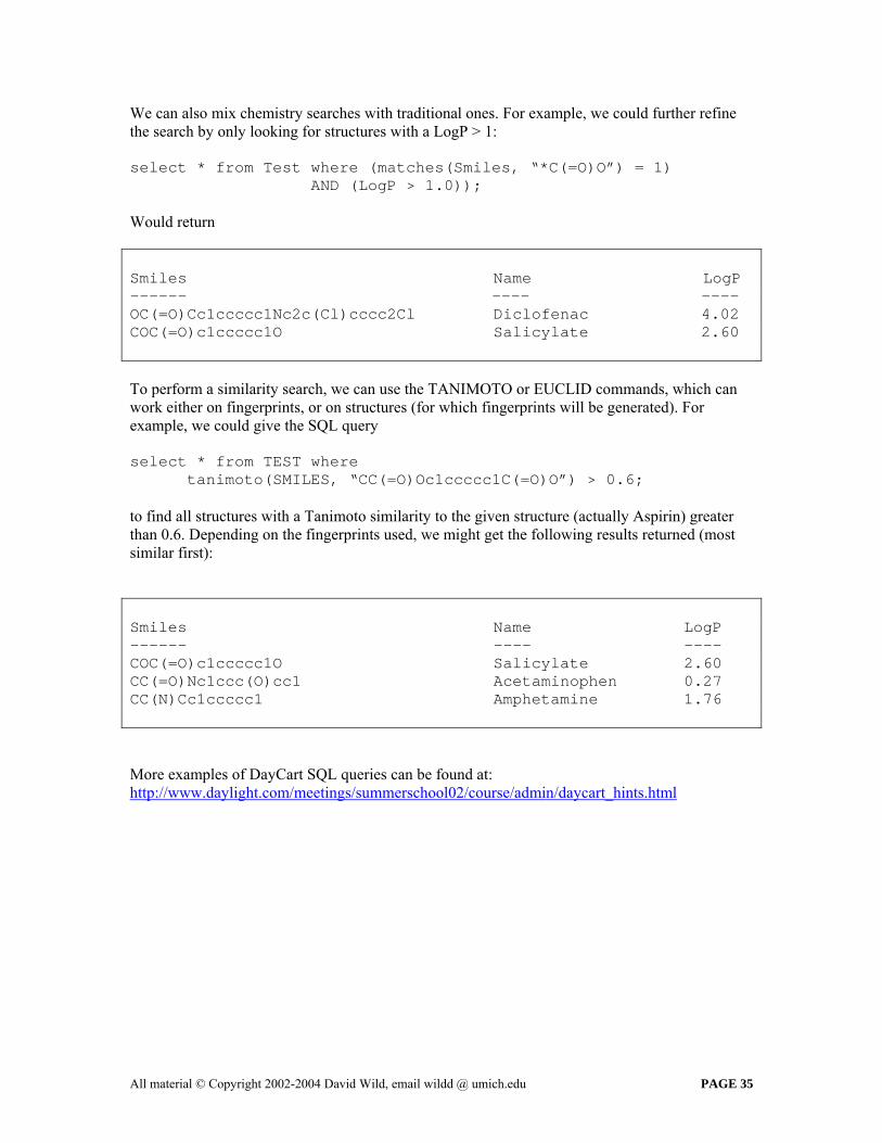
We can also mix chemistry searches with traditional ones. For example, we could further refine the search by only looking for structures with a LogP > 1: select * from Test where (matches(Smiles, “*C(=O)O”) = 1) AND (LogP > 1.0)); Would return Smiles Name LogP ------ ---- ---- OC(=O)Cc1ccccc1Nc2c(Cl)cccc2Cl Diclofenac 4.02 COC(=O)c1ccccc1O Salicylate 2.60 To perform a similarity search, we can use the TANIMOTO or EUCLID commands, which can work either on fingerprints, or on structures (for which fingerprints will be generated). For example, we could give the SQL query select * from TEST where tanimoto(SMILES, “CC(=O)Oc1ccccc1C(=O)O”) > 0.6; to find all structures with a Tanimoto similarity to the given structure (actually Aspirin) greater than 0.6. Depending on the fingerprints used, we might get the following results returned (most similar first): Smiles Name LogP ------ ---- ---- COC(=O)c1ccccc1O Salicylate 2.60 CC(=O)Nc1ccc(O)cc1 Acetaminophen 0.27 CC(N)Cc1ccccc1 Amphetamine 1.76 More examples of DayCart SQL queries can be found at: http://www.daylight.com/meetings/summerschool02/course/admin/daycart_hints.html


http://www.daylight.com/meetings/summerschool02/course/admin/daycart_hints.html

http://www.daylight.com/meetings/summerschool02/course/admin/daycart_hints.html

7. Online demonstrations of 2D searching There are at least two online searching engines that are worthy of note. Firstly, check out the Molinspiration search engine at http://www.molinspiration.com/cgi-bin/search for a nice demonstration search tool that uses the JME interface. Secondly, take a look at http://cactus.nci.nih.gov where the CACTVS drawing and searching technology from Erlangen has been used to allow searching of the large (>250,000 structure) NCI database. 8. 3D searching 3D searching is less used that 2D searching. 3D databases store coordinate tables and usually distance matrices for all molecules. 3D searching techniques are less “mature” than 2D searching, and are generally used for different purposes. Also, 3D searching needs to take into account conformational flexibility. There are two common types of 3D search – the pharmacophore search and 3D similarity search. Pharmacophore Search A pharmacophore is a definition of the 3D features a molecule needs in order to bind to a protein active site. For example, the following pharmacophore specifies the features that might be required for binding to the protein active site (shown in green). The requirement is for any molecule fitting the pharmacophore to have an OH group between 2 and 5 Å away from a Carboxyl Oxygen, both of which are 7-8 Å from a Benzene Ring.

OH

A pharmacophore search would use the distance matrix representation to look for molecules that would fit this pattern. For example, the following molecule could be returned by the search:

OH

C

O 7-8 Å

7-8 Å

2-5 Å

HO

Protein Surface

C

O

2-5 Å

7-8 Å

7-8 Å

Protein Surface


http://www.molinspiration.com/cgi-bin/search

http://cactus.nci.nih.gov/

Note that we haven’t considered flexibility of the molecule here – that’s a further complication! 3D Similarity Search There are a number of ways of similarity searching 3D databases. The most common are: • Using 3D fingerprints based on pharmacophore “fragments” (and then using measures such

as Tanimoto or Euclidean Distance on the fingerprints). For an example, see Comparing 3D Pharmacophore Triplets and 2D Fingerprints for Selecting Diverse Compound Subsets. H. Matter and T. Pötter, J. Chem. Inf. Comput. Sci.; 1999; 39(6) pp 1211 – 1225, available at http://pubs3.acs.org/acs/journals/doilookup?in_doi=10.1021/ci980185h

• Using atom-based methods of similarity, involving comparison of distance matrices. For

example, finding pairs of most-similar atoms between molecules, based on their distances from other atoms in the molecule

• Using fields or surface representations. For example, see Calculation of Structural Similarity

by the Alignment of Molecular Electrostatic Potentials, D. Thorner, D. Wild, P. Willett, & M. Wright, Perspectives in Drug Discovery and Design, 9/10/11, 301-320, 1998, available at http://ipsapp008.lwwonline.com/content/getfile/5072/1/17/abstract.htm

3D similarity searches are used both for searching databases and for ranking small datasets (by the similarity measure). There is a fair debate over which is best – 2D or 3D. General consensus is that for most searching applications (particularly involving large numbers of compounds) 2D is the most useful, but for small datasets and some specific applications (particularly searching for bioisosteres, novel compounds that may be from a different series but could exhibit similar activity to a query), 3D can be more effective. For a good overview of 3D databases, see the Network Science review at http://www.netsci.org/Science/Cheminform/feature06.html. 9. Protein searching This won’t be covered in detail, but a number of programs exist for finding similar protein structures to a query. Indeed this is the basis of homology modeling. See, for example, BLAST, which “aligns” primary structures and calculates a similarity value: http://www.ncbi.nlm.nih.gov/BLAST/blast_overview.html.


http://pubs3.acs.org/acs/journals/doilookup?in_doi=10.1021/ci980185h




http://ipsapp008.lwwonline.com/content/getfile/5072/1/17/abstract.htm




http://www.netsci.org/Science/Cheminform/feature06.html

http://www.ncbi.nlm.nih.gov/BLAST/blast_overview.html

5. ADVANCED CHEMOINFORMATICS METHODS

Learning Objectives: • Know the three main applications of cluster-analysis • Understand how Ward’s, K-means and Jarvis-Patrick clustering methods work • Understand the terms “descriptor space”, “chemistry space” and “drug space” • Understand how the diversity of a dataset and between datasets may be calculated • Understand how a diverse subset might be selected • Know the three phases in building a computational SAR model • Understand how Recursive Partitioning works • Know about methods used for ADME/Tox Prediction

1. Cluster Analysis This term refers to a group of statistical methods used for identifying groups (“clusters”) of similar items in a multi-dimensional space. Cluster analysis can be used whenever we have a measure of similarity between two items available. We can understand what cluster analysis does if we use an imaginary 2D space (although we would normally have many more dimensions than two):

In this diagram, the small blue circles represent items plotted in the 2D space, and the red circles represent “clusters” found by a clustering algorithm. Note that it’s not always clear what the “natural” clusters are (e.g. should the rightmost two clusters be one?) and some points are not placed in clusters (“singletons”).


Cluster analysis has three main uses in chemoinformatics:

• Grouping compounds into chemical series, which particularly helpful in analyzing large datsets (i.e. 1,000 series easier to analyze than 50,000 arbitrary compounds)

• Grouping structures which are likely to have similar biological activity, the premise being that if several compounds in a cluster are active, others are likely to be active too

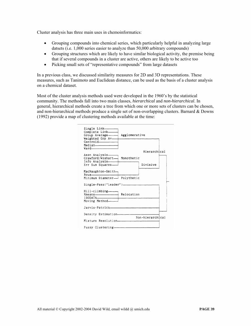
• Picking small sets of “representative compounds” from large datasets In a previous class, we discussed similarity measures for 2D and 3D representations. These measures, such as Tanimoto and Euclidean distance, can be used as the basis of a cluster analysis on a chemical dataset. Most of the cluster analysis methods used were developed in the 1960’s by the statistical community. The methods fall into two main classes, hierarchical and non-hierarchical. In general, hierarchical methods create a tree from which one or more sets of clusters can be chosen, and non-hierarchical methods produce a single set of non-overlapping clusters. Barnard & Downs (1992) provide a map of clustering methods available at the time:


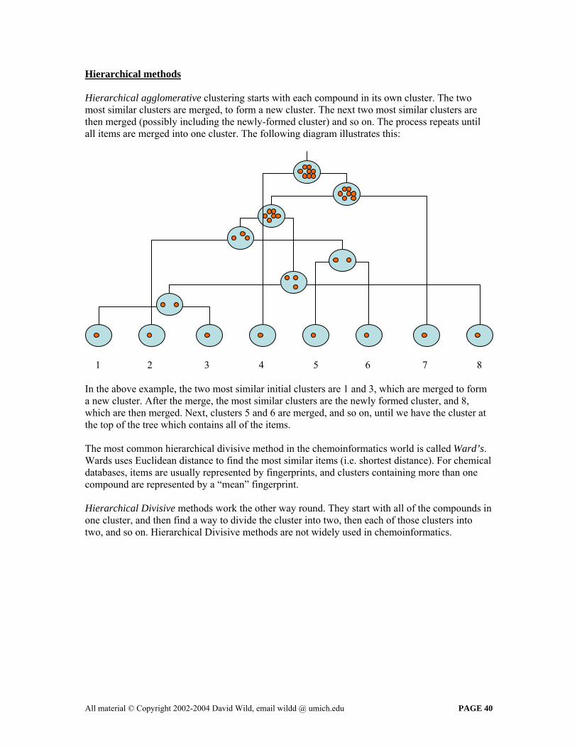
Hierarchical methods Hierarchical agglomerative clustering starts with each compound in its own cluster. The two most similar clusters are merged, to form a new cluster. The next two most similar clusters are then merged (possibly including the newly-formed cluster) and so on. The process repeats until all items are merged into one cluster. The following diagram illustrates this:

1 2 3 4 5 6 7 8 In the above example, the two most similar initial clusters are 1 and 3, which are merged to form a new cluster. After the merge, the most similar clusters are the newly formed cluster, and 8, which are then merged. Next, clusters 5 and 6 are merged, and so on, until we have the cluster at the top of the tree which contains all of the items. The most common hierarchical divisive method in the chemoinformatics world is called Ward’s. Wards uses Euclidean distance to find the most similar items (i.e. shortest distance). For chemical databases, items are usually represented by fingerprints, and clusters containing more than one compound are represented by a “mean” fingerprint. Hierarchical Divisive methods work the other way round. They start with all of the compounds in one cluster, and then find a way to divide the cluster into two, then each of those clusters into two, and so on. Hierarchical Divisive methods are not widely used in chemoinformatics.


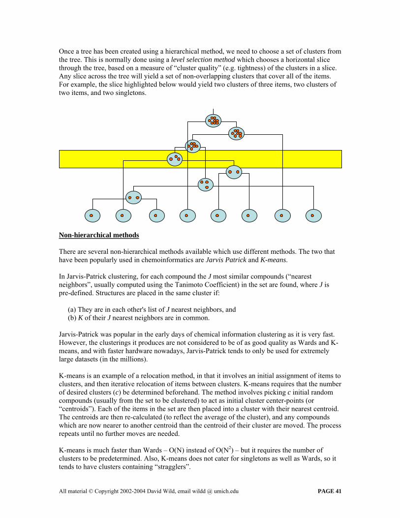
Once a tree has been created using a hierarchical method, we need to choose a set of clusters from the tree. This is normally done using a level selection method which chooses a horizontal slice through the tree, based on a measure of “cluster quality” (e.g. tightness) of the clusters in a slice. Any slice across the tree will yield a set of non-overlapping clusters that cover all of the items. For example, the slice highlighted below would yield two clusters of three items, two clusters of two items, and two singletons.

Non-hierarchical methods There are several non-hierarchical methods available which use different methods. The two that have been popularly used in chemoinformatics are Jarvis Patrick and K-means. In Jarvis-Patrick clustering, for each compound the J most similar compounds (“nearest neighbors”, usually computed using the Tanimoto Coefficient) in the set are found, where J is pre-defined. Structures are placed in the same cluster if: (a) They are in each other's list of J nearest neighbors, and (b) K of their J nearest neighbors are in common. Jarvis-Patrick was popular in the early days of chemical information clustering as it is very fast. However, the clusterings it produces are not considered to be of as good quality as Wards and K-means, and with faster hardware nowadays, Jarvis-Patrick tends to only be used for extremely large datasets (in the millions). K-means is an example of a relocation method, in that it involves an initial assignment of items to clusters, and then iterative relocation of items between clusters. K-means requires that the number of desired clusters (c) be determined beforehand. The method involves picking c initial random compounds (usually from the set to be clustered) to act as initial cluster center-points (or “centroids”). Each of the items in the set are then placed into a cluster with their nearest centroid. The centroids are then re-calculated (to reflect the average of the cluster), and any compounds which are now nearer to another centroid than the centroid of their cluster are moved. The process repeats until no further moves are needed. K-means is much faster than Wards – O(N) instead of O(N2) – but it requires the number of clusters to be predetermined. Also, K-means does not cater for singletons as well as Wards, so it tends to have clusters containing “stragglers”.


“New” Methods In the last ten years or so, the requirements of the data-mining community have meant that more

done on clustering, and more methods have been developed, which get round ome of the weaknesses of traditional clustering methods (such as not being able to handle oddly-

Sci., 1998, 38, 983-996 • Clustering of Chemical Structures on the Basis of Two-Dimensional Similarity Measures,

• in Computational Chemistry, G.M.Downs and J. M.

For ta

• Separating Actives and Inactives Clustering Methods

and Descriptors for Use in Compound Selection, R.D. Brown, Y.C. Martin, J. 996, 36, 572-584.

• Finding

– rarchy Level Selection Methods for Structural Grouping using Wards Clustering, D.J. Wild, J. Blankley, J. Chem. Inf.

t. Sci., 2000, 40, 155-162. BCI Ltd. producMeans and Jarv e their website at http://www.bci.gb.com

research has beensshaped clusters well). Examples are ROCK, CURE, and Chameleon. These methods are currentlyunder evaluation for application in chemical information. For more information, see the 2002 Downs & Barnard paper. For a more detailed review of clustering techniques, see the following papers (available on thecourse website):

• Chemical Similarity Searching, P. Willett, J.M. Barnard, G.M.Downs, J. Chem. Inf. Comput.

J. Chem. Inf. Comput. Sci, 1992, 36, 644-649 Clustering methods and their usesBarnard, Reviews in Computational Chemistry, 2002, 18, 1-40

de ils of the application of these methods to grouping compounds, see:

– Use of Structure-Activity Data to Compare Structure-Based

Chem. Inf. Comput. Sci., 1

series Comparison of 2D Fingerprint Types and Hie

Compu

e a number of clustering programs for Windows and Unix, including Ward’s, K-is-Patrick. For more information, se .


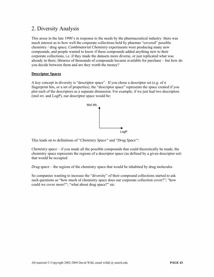
2. Diversity Analysis This arose in the late 1990’s in response to the needs by the pharmaceutical industry: there was much interest as to how well the corporate collections held by pharmas “covered” possible chemistry / drug space; Combinatorial Chemistry experiments were producing many new compounds, and people wanted to know if these compounds added anything new to their corporate collections, i.e. if they made the datasets more diverse, or just replicated what was already in there; libraries of thousands of compounds became available for purchase – but how do you decide between them and are they worth the money? Descriptor Spaces A key concept in diversity is “descriptor space”. If you chose a descriptor set (e.g. of n fingerprint bits, or a set of properties), the “descriptor space” represents the space created if you plot each of the descriptors as a separate dimension. For example, if we just had two descriptors (mol.wt. and LogP), our descriptor space would be:

Mol Wt.

LogP

This leads on to definitions of “Chemistry Space” and “Drug Space”: Chemistry space – if you made all the possible compounds that could theoretically be made, the chemistry space represents the regions of a descriptor space (as defined by a given descriptor set) that would be occupied Drug space – the regions of the chemistry space that would be inhabited by drug molecules So companies wanting to increase the “diversity” of their compound collections started to ask such questions as “how much of chemistry space does our corporate collection cover?”; “how could we cover more?”; “what about drug space?” etc


Measuring Diversity One of the main methods for measuring the diversity of a dataset is the mean dissimilarity method. This involves calculating the Mean Inter-molecular Similarity of all the pairs of molecules in the set, e.g. using the tanimoto coefficient:

where there are n compounds in the dataset, and Tij

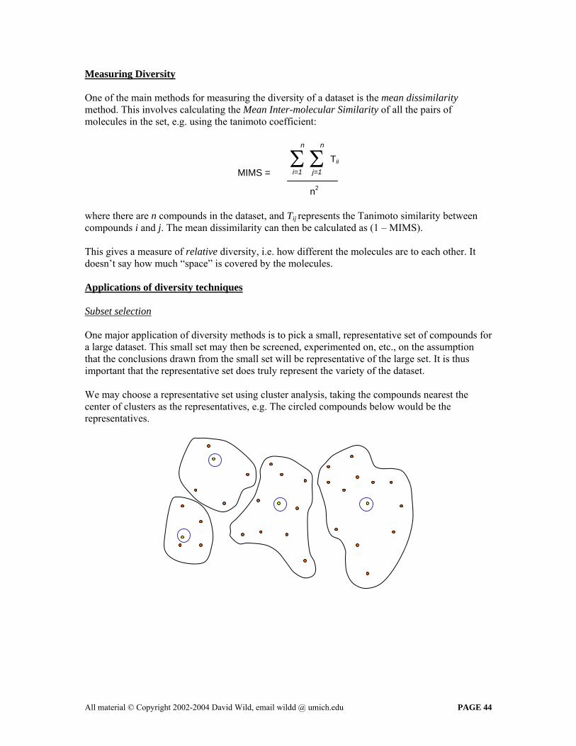
represents the Tanimoto similarity between compounds i and j. The mean dissimilarity can then be calculated as (1 – MIMS). This gives a measure of relative diversity, i.e. how different the molecules are to each other. It doesn’t say how much “space” is covered by the molecules. Applications of diversity techniques Subset selection One major application of diversity methods is to pick a small, representative set of compounds for a large dataset. This small set may then be screened, experimented on, etc., on the assumption that the conclusions drawn from the small set will be representative of the large set. It is thus important that the representative set does truly represent the variety of the dataset. We may choose a representative set using cluster analysis, taking the compounds nearest the center of clusters as the representatives, e.g. The circled compounds below would be the representatives.

MIMS = Σ Tij

j=1

n

Σn

i=1

n2


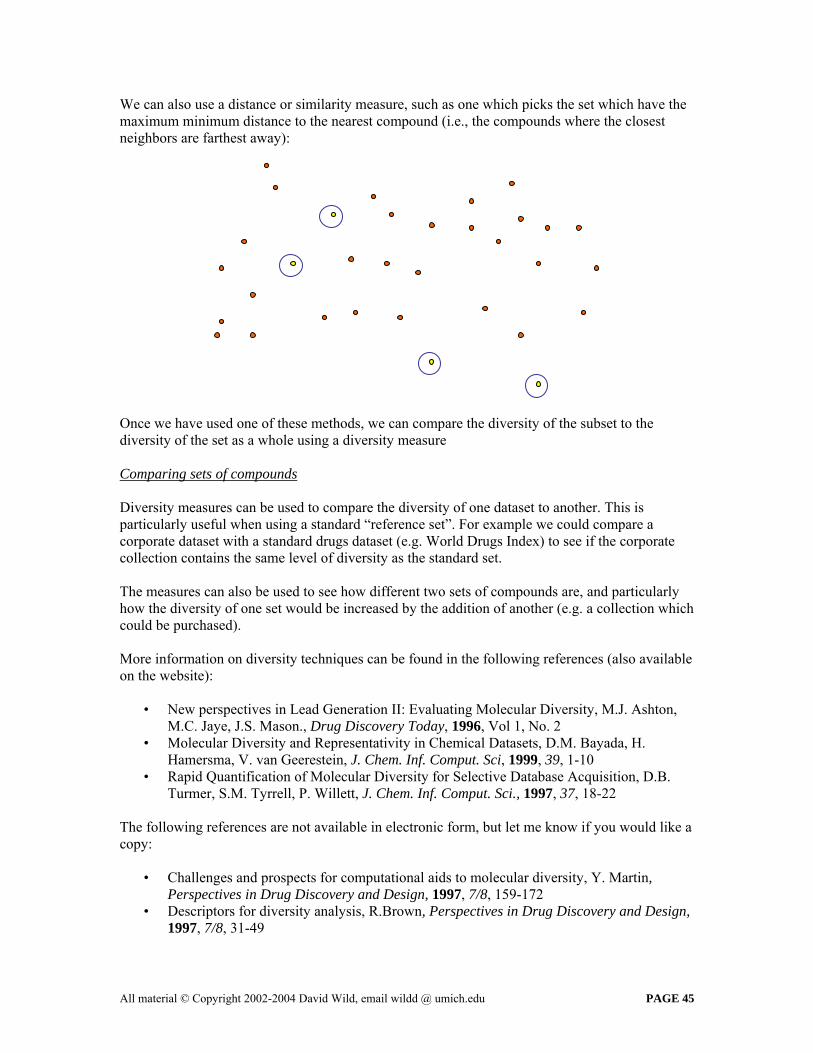
We can also use a distance or similarity measure, such as one which picks the set which have the maximum minimum distance to the nearest compound (i.e., the compounds where the closest neighbors are farthest away):

Once we have used one of these methods, we can compare the diversity of the subset to the diversity of the set as a whole using a diversity measure Comparing sets of compounds Diversity measures can be used to compare the diversity of one dataset to another. This is particularly useful when using a standard “reference set”. For example we could compare a corporate dataset with a standard drugs dataset (e.g. World Drugs Index) to see if the corporate collection contains the same level of diversity as the standard set. The measures can also be used to see how different two sets of compounds are, and particularly how the diversity of one set would be increased by the addition of another (e.g. a collection which could be purchased). More information on diversity techniques can be found in the following references (also available on the website):

• New perspectives in Lead Generation II: Evaluating Molecular Diversity, M.J. Ashton, M.C. Jaye, J.S. Mason., Drug Discovery Today, 1996, Vol 1, No. 2

• Molecular Diversity and Representativity in Chemical Datasets, D.M. Bayada, H. Hamersma, V. van Geerestein, J. Chem. Inf. Comput. Sci, 1999, 39, 1-10

• Rapid Quantification of Molecular Diversity for Selective Database Acquisition, D.B. Turmer, S.M. Tyrrell, P. Willett, J. Chem. Inf. Comput. Sci., 1997, 37, 18-22

The following references are not available in electronic form, but let me know if you would like a copy:

• Challenges and prospects for computational aids to molecular diversity, Y. Martin, Perspectives in Drug Discovery and Design, 1997, 7/8, 159-172

• Descriptors for diversity analysis, R.Brown, Perspectives in Drug Discovery and Design, 1997, 7/8, 31-49


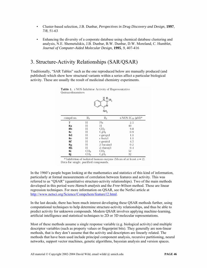
• Cluster-based selection, J.B. Dunbar, Perspectives in Drug Discovery and Design, 1997, 7/8, 51-63

• Enhancing the diversity of a corporate database using chemical database clustering and

analysis, N.E. Shemetulskis, J.B. Dunbar, B.W. Dunbar, D.W. Moreland, C. Humblet, Journal of Computer-Aided Molecular Design, 1995, 9, 407-416

3. Structure-Activity Relationships (SAR/QSAR) Traditionally, “SAR Tables” such as the one reproduced below are manually produced (and published) which show how structural variants within a series affect a particular biological activity. These are usually the result of medicinal chemistry experiments.

In the 1960’s people began looking at the mathematics and statistics of this kind of information, particularly at formal measurements of correlation between features and activity. This was referred to as “QSAR” (quantitative structure-activity relationships). Two of the main methods developed in this period were Hansch analysis and the Free-Wilson method. These are linear regression techniques. For more information on QSAR, see the NetSci article at http://www.netsci.org/Science/Compchem/feature12.html. In the last decade, there has been much interest developing these QSAR methods further, using computational techniques to help determine structure-activity relationships, and thus be able to predict activity for unknown compounds. Modern QSAR involves applying machine-learning, artificial intelligence and statistical techniques to 2D or 3D molecular representations. Most of these methods assume a single response variable (e.g. biological activity) and multiple descriptor variables (such as property values or fingerprint bits). They generally are non-linear methods, that is they don’t assume that the activity and descriptors are linearly related. The methods that have been used include principal component analysis, recursive partitioning, neural networks, support vector machines, genetic algorithms, bayesian analysis and version spaces.


http://www.netsci.org/Science/Compchem/feature12.html

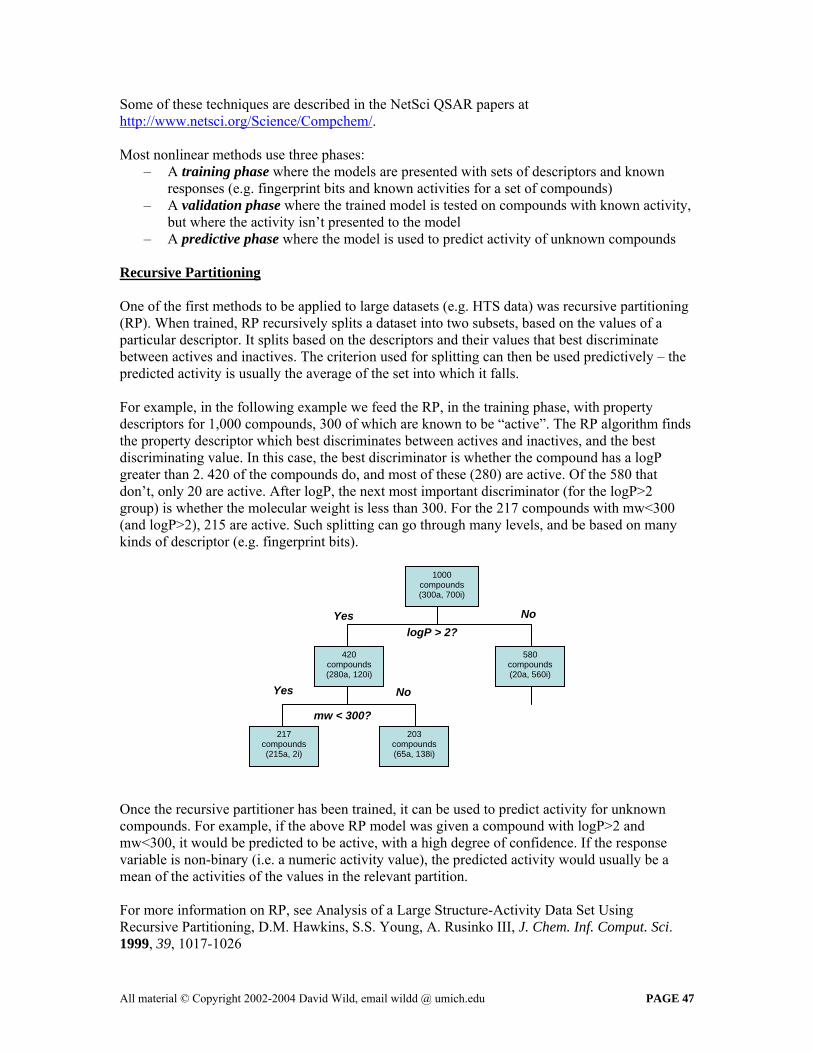
Some of these techniques are described in the NetSci QSAR papers at http://www.netsci.org/Science/Compchem/. Most nonlinear methods use three phases:

are presented with sets of descriptors and known

– wn activity,

– ict activity of unknown compounds

ecursive Partitioning

– A training phase where the modelsresponses (e.g. fingerprint bits and known activities for a set of compounds) A validation phase where the trained model is tested on compounds with knobut where the activity isn’t presented to the model A predictive phase where the model is used to pred

R

ne of the first methods to be applied to large datasets (e.g. HTS data) was recursive partitioning

the

or example, in the following example we feed the RP, in the training phase, with property

00

nce the recursive partitioner has been trained, it can be used to predict activity for unknown

se

or more information on RP, see Analysis of a Large Structure-Activity Data Set Using Recursive Partitioning, D.M. Hawkins, S.S. Young, A. Rusinko III, J. Chem. Inf. Comput. Sci. 1999, 39, 1017-1026

O(RP). When trained, RP recursively splits a dataset into two subsets, based on the values of a particular descriptor. It splits based on the descriptors and their values that best discriminate between actives and inactives. The criterion used for splitting can then be used predictively –predicted activity is usually the average of the set into which it falls. Fdescriptors for 1,000 compounds, 300 of which are known to be “active”. The RP algorithm finds the property descriptor which best discriminates between actives and inactives, and the best discriminating value. In this case, the best discriminator is whether the compound has a logPgreater than 2. 420 of the compounds do, and most of these (280) are active. Of the 580 that don’t, only 20 are active. After logP, the next most important discriminator (for the logP>2 group) is whether the molecular weight is less than 300. For the 217 compounds with mw<3(and logP>2), 215 are active. Such splitting can go through many levels, and be based on many kinds of descriptor (e.g. fingerprint bits).

1000 compounds (300a, 700i)

logP > 2? No Yes

420 compou

580 compounds

(280a, 120i) nds

(20a, 560i)

mw < 300? 217

compou

Yes No

203 compounds

(215a, 2i) nds

(65a, 138i)

Ocompounds. For example, if the above RP model was given a compound with logP>2 and mw<300, it would be predicted to be active, with a high degree of confidence. If the responvariable is non-binary (i.e. a numeric activity value), the predicted activity would usually be a mean of the activities of the values in the relevant partition. F


http://www.netsci.org/Science/Compchem/

4. ADME/Tox Prediction ADME stands for Absorbtion, Distribthe main factors involved in the intake

ution, Metabolism and Excretion, and refers to the study of , processing and excretion of drugs in the body. “Tox”

fers to prediction of toxicity. Traditionally, animals were used for pre-human testing. However, reanimal tests are expensive, time consuming and ethically undesirable. ADME/Tox techniques help model how the drug will likely act in the body These methods can be experemental (in vitro) using cellular tissue, or in silico, using computational models In-vitro ADME models These models are based around real tissue samples, which have similar properties to those in the

O-2 tissue closely resembles the lining of the stomach, so if a molecule asses through CACO-2 it likely will also pass through the stomach lining, and thus be a

body. For example, CACpcandidate for oral delivery. In-vitro ADME cuts down animal tests, by acting as a “pre-screen”, and enables ADME data to be discovered on many more compounds than used to be possible. In-silico ADME models Computational methods can be used to predict compound properties important to ADME, e.g.

solubility, permeability, phase I metabolism. Since these are urely computational, estimates can be made for millions of compouds, helping reduce “attrition”

LogP, a liphophilicity measure, p– the failure rate of compounds in late stage. LogP Calculation LogP methods tend to use databases of experimental lipophilicity values for fragments. A logP

ted additively from these partial lipophilicities. Early work by Hansch & Leo roduced fragment lookup tables. For an example of the use of these. see e.g., Molecular

can then be calculapStructures: perception, autocorrelation, descriptor and sar studies, P. Broto et. al., Eur. J. Med. Chem. – Chem. Ther, 1984, 19, no 1, pp71-78 (copy available – email me).

Solubility Calculation These tend to use a linear equation incorporating lipophilicity, molar refractivity, polarity,

basicity terms. For example, the Abraham equation:

C – constant of the equation

S – solute dipolarity/polarisability dity

volume, acidity, and/or Log(Sw) = c + eE + sS + aA + bB + vV E - solute excess molar refraction A – solute hydrogen bond aci B – solute hydrogen bond basicity V – McGowan volume


Metabolism Prediction Cytochrome p450 (CP450) is a superfamily of proteins involved in phase I metabolism. The 3D structures for many of these enzymes have been determined, and for those we can use a docking experiment to predict binding to the enzyme (and thus a probability of metabolism occurring). For those where a structure is not available, a pharmacophore model can be used. For more information on ADME models, see the NetSci article at http://www.netsci.org/Science/Special/feature06.html. A simple property calculation engine is available on the web at http://www.molinspiration.com/cgi-bin/properties. Toxicity Prediction These methods predict whether a compound is likely to be toxic to animals or humans. It can be hard to get data, because companies don’t publish “bad” data, and even within companies the data is often hard to obtain. Simple or complex methods can be used. An example of a simple method would be keeping a list of SMARTS of “toxicophores” to screen against compounds. An example of a more advanced method would be the use of machine-learning techniques like RP or neural nets – fed with training set containing toxic and non-toxic substances


a brief introduction to chemoinformatics relationships (sar/qsar) ... researchers in the us...

Documents