a brief introduction to kernel classifiers - brown university
TRANSCRIPT
A brief introduction to kernel classifiers
Mark JohnsonBrown University
October 2009
1 / 21
Outline
Introduction
Linear and nonlinear classifiers
Kernels and classifiers
The kernelized perceptron learner
Conclusions
2 / 21
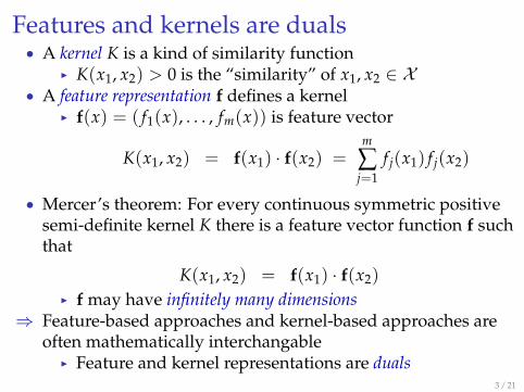
Features and kernels are duals• A kernel K is a kind of similarity function
I K(x1, x2) > 0 is the “similarity” of x1, x2 ∈ X• A feature representation f defines a kernel
I f(x) = ( f1(x), . . . , fm(x)) is feature vector
K(x1, x2) = f(x1) · f(x2) =m
∑j=1
f j(x1) f j(x2)
• Mercer’s theorem: For every continuous symmetric positivesemi-definite kernel K there is a feature vector function f suchthat
K(x1, x2) = f(x1) · f(x2)I f may have infinitely many dimensions
⇒ Feature-based approaches and kernel-based approaches areoften mathematically interchangable
I Feature and kernel representations are duals3 / 21

Learning algorithms and kernels
• Feature representations and kernel representations are duals⇒ Many learning algorithms can use either features or kernels
I feature version maps examples into feature space andlearns feature statistics
I kernel version uses “similarity” between this exampleand other examples, and learns example statistics
• Both versions learn same classification function• Computational complexity of feature vs kernel algorithms can
vary dramaticallyI few features, many training examples⇒ feature version may be more efficient
I few training examples, many features⇒ kernel version may be more efficient
4 / 21
Outline
Introduction
Linear and nonlinear classifiers
Kernels and classifiers
The kernelized perceptron learner
Conclusions
5 / 21
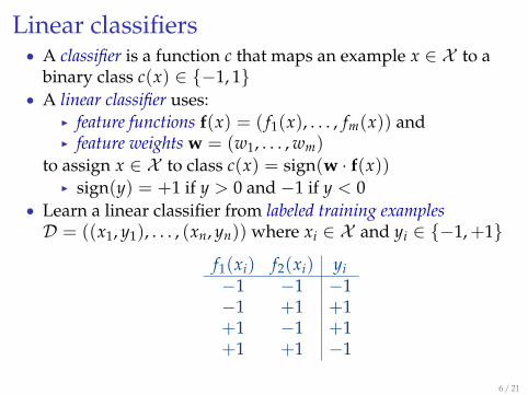
Linear classifiers• A classifier is a function c that maps an example x ∈ X to a
binary class c(x) ∈ {−1, 1}• A linear classifier uses:
I feature functions f(x) = ( f1(x), . . . , fm(x)) andI feature weights w = (w1, . . . , wm)
to assign x ∈ X to class c(x) = sign(w · f(x))I sign(y) = +1 if y > 0 and −1 if y < 0
• Learn a linear classifier from labeled training examplesD = ((x1, y1), . . . , (xn, yn)) where xi ∈ X and yi ∈ {−1, +1}
f1(xi) f2(xi) yi−1 −1 −1−1 +1 +1+1 −1 +1+1 +1 −1
6 / 21
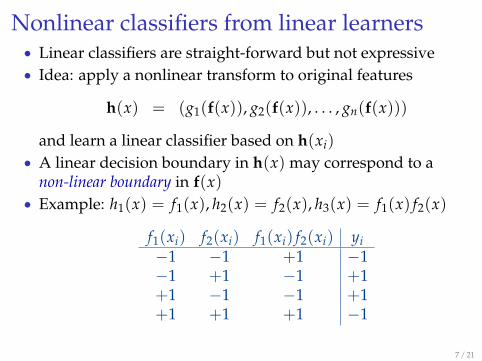
Nonlinear classifiers from linear learners• Linear classifiers are straight-forward but not expressive• Idea: apply a nonlinear transform to original features
h(x) = (g1(f(x)), g2(f(x)), . . . , gn(f(x)))
and learn a linear classifier based on h(xi)• A linear decision boundary in h(x) may correspond to a
non-linear boundary in f(x)• Example: h1(x) = f1(x), h2(x) = f2(x), h3(x) = f1(x) f2(x)
f1(xi) f2(xi) f1(xi) f2(xi) yi−1 −1 +1 −1−1 +1 −1 +1+1 −1 −1 +1+1 +1 +1 −1
7 / 21
Outline
Introduction
Linear and nonlinear classifiers
Kernels and classifiers
The kernelized perceptron learner
Conclusions
8 / 21

Linear classifiers using kernels• Linear classifier decision rule: Given feature functions f and
weights w, assign x ∈ X to class
c(x) = sign(w · f(x))
• Linear kernel using features f: for all u, v ∈ X
K(u, v) = f(u) · f(v)
• The kernel trick: Assume w = ∑nk=1 sk f(xk),
i.e., the feature weights w are represented implicitly byexamples (x1, . . . , xn). Then:
c(x) = sign(n
∑k=1
sk f(xk) · f(x))
= sign(n
∑k=1
sk K(xk, x))
9 / 21
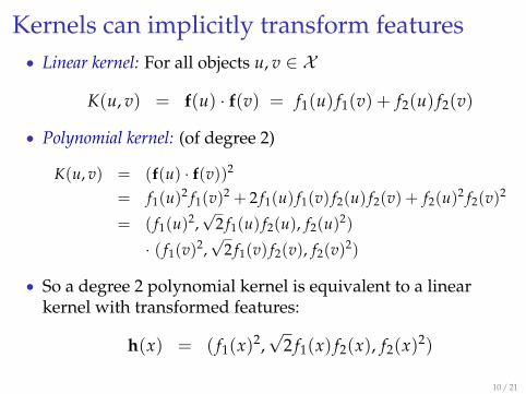
Kernels can implicitly transform features• Linear kernel: For all objects u, v ∈ X
K(u, v) = f(u) · f(v) = f1(u) f1(v) + f2(u) f2(v)
• Polynomial kernel: (of degree 2)
K(u, v) = (f(u) · f(v))2
= f1(u)2 f1(v)2 + 2 f1(u) f1(v) f2(u) f2(v) + f2(u)2 f2(v)2
= ( f1(u)2,√
2 f1(u) f2(u), f2(u)2)
· ( f1(v)2,√
2 f1(v) f2(v), f2(v)2)
• So a degree 2 polynomial kernel is equivalent to a linearkernel with transformed features:
h(x) = ( f1(x)2,√
2 f1(x) f2(x), f2(x)2)
10 / 21
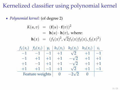
Kernelized classifier using polynomial kernel
• Polynomial kernel: (of degree 2)
K(u, v) = (f(u) · f(v))2
= h(u) · h(v), where:
h(x) = ( f1(x)2,√
2 f1(x) f2(x), f2(x)2)
f1(xi) f2(xi) yi h1(xi) h2(xi) h3(xi) si−1 −1 −1 +1
√2 +1 −1
−1 +1 +1 +1 −√
2 +1 +1+1 −1 +1 +1 −
√2 +1 +1
+1 +1 −1 +1√
2 +1 −1Feature weights 0 −2
√2 0
11 / 21
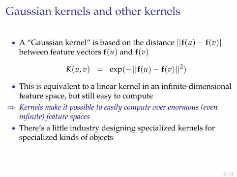
Gaussian kernels and other kernels
• A “Gaussian kernel” is based on the distance ||f(u)− f(v)||between feature vectors f(u) and f(v)
K(u, v) = exp(−||f(u)− f(v)||2)
• This is equivalent to a linear kernel in an infinite-dimensionalfeature space, but still easy to compute
⇒ Kernels make it possible to easily compute over enormous (eveninfinite) feature spaces
• There’s a little industry designing specialized kernels forspecialized kinds of objects
12 / 21
Mercer’s theorem
• Mercer’s theorem: every continuous symmetric positivesemi-definite kernel is a linear kernel in some feature space
I this feature space may be infinite-dimensional• This means that:
I feature-based linear classifiers can often be expressed askernel-based classifiers
I kernel-based classifiers can often be expressed asfeature-based linear classifiers
13 / 21
Outline
Introduction
Linear and nonlinear classifiers
Kernels and classifiers
The kernelized perceptron learner
Conclusions
14 / 21
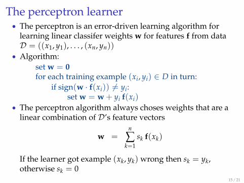
The perceptron learner• The perceptron is an error-driven learning algorithm for
learning linear classifer weights w for features f from dataD = ((x1, y1), . . . , (xn, yn))
• Algorithm:set w = 0for each training example (xi, yi) ∈ D in turn:
if sign(w · f(xi)) 6= yi:set w = w + yi f(xi)
• The perceptron algorithm always choses weights that are alinear combination of D’s feature vectors
w =n
∑k=1
sk f(xk)
If the learner got example (xk, yk) wrong then sk = yk,otherwise sk = 0
15 / 21
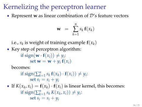
Kernelizing the perceptron learner• Represent w as linear combination of D’s feature vectors
w =n
∑k=1
sk f(xk)
i.e., sk is weight of training example f(xk)• Key step of perceptron algorithm:
if sign(w · f(xi)) 6= yi:set w = w + yi f(xi)
becomes:if sign(∑n
k=1 sk f(xk) · f(xi)) 6= yi:set si = si + yi
• If K(xk, xi) = f(xk) · f(xi) is linear kernel, this becomes:if sign(∑n
k=1 sk K(xk, xi)) 6= yi:set si = si + yi
16 / 21
Kernelized perceptron learner
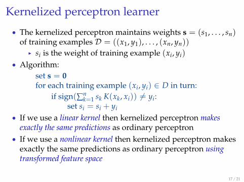
• The kernelized perceptron maintains weights s = (s1, . . . , sn)of training examples D = ((x1, y1), . . . , (xn, yn))
I si is the weight of training example (xi, yi)• Algorithm:
set s = 0for each training example (xi, yi) ∈ D in turn:
if sign(∑nk=1 sk K(xk, xi)) 6= yi:
set si = si + yi
• If we use a linear kernel then kernelized perceptron makesexactly the same predictions as ordinary perceptron
• If we use a nonlinear kernel then kernelized perceptron makesexactly the same predictions as ordinary perceptron usingtransformed feature space
17 / 21

Gaussian-regularized MaxEnt models• Given data D = ((x1, y1), . . . , (xn, yn)), the weights w that
maximize the Gaussian-regularized conditional log likelihood are:
w = argminw
Q(w) where:
Q(w) = − log LD(w) + αm
∑k=1
w2k
∂Q∂wj
=n
∑i=1−( f j(xi, yi)− Ew[ f j | xi]) + 2αwj
• Because ∂Q/∂wj = 0 at w = w, we have:
wj =1
2α
n
∑i=1
( f j(yi, xi)− Ew[ f j | xi])
18 / 21
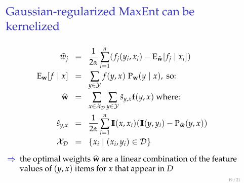
Gaussian-regularized MaxEnt can bekernelized
wj =1
2α
n
∑i=1
( f j(yi, xi)− Ew[ f j | xi])
Ew[ f | x] = ∑y∈Y
f (y, x) Pw(y | x), so:
w = ∑x∈XD
∑y∈Y
sy,xf(y, x) where:
sy,x =1
2α
n
∑i=1
II(x, xi)(II(y, yi)− Pw(y, x))
XD = {xi | (xi, yi) ∈ D}
⇒ the optimal weights w are a linear combination of the featurevalues of (y, x) items for x that appear in D
19 / 21
Outline
Introduction
Linear and nonlinear classifiers
Kernels and classifiers
The kernelized perceptron learner
Conclusions
20 / 21

Conclusions• Many algorithms have dual forms using feature and kernel
representations• For any feature representation there is an equivalent kernel• For any sensible kernel there is an equivalent feature
representationI but the feature space may be infinite dimensional
• There can be substantial computational advantages to usingfeatures or kernels
I many training examples, few features⇒ features may be more efficient
I many features, few training examples⇒ kernels may be more efficient
• Kernels make it possible to compute with very large (eveninfinite-dimensional) feature spaces, but each classification requirescomparing to a potentially large number of training examples
21 / 21