a branch-and-bound algorithm for the close-enough ... · a branch-and-bound algorithm for the...
TRANSCRIPT
A Branch-and-Bound Algorithm for theClose-Enough Traveling Salesman Problem
Walton Pereira Coutinho, Anand SubramanianDepartamento de Engenharia de Producao, Centro de Tecnologia — Universidade Federal da Paraıba
Campus I, Bloco G, Cidade Universitaria, 58051-970, Joao Pessoa - PB, Brazil
[email protected], [email protected]
Roberto Quirino do NascimentoDepartamento de Computacao Cientıfica, Centro de Informatica — Universidade Federal da Paraıba
Campus I, Bloco G, Cidade Universitaria, 58051-970, Joao Pessoa - PB, Brazil
Artur Alves PessoaDepartamento de Engenharia de Producao — Universidade Federal Fluminense
Rua Passo da Patria, 156, Bloco E, 4 andar, Sao Domingos, 24210-240, Niteroi - RJ, Brazil
This paper deals with the Close-Enough Traveling Salesman Problem (CETSP). In the CETSP, rather than
visiting the vertex (customer) itself, the salesman must visit a specific region containing such vertex. To solve
this problem, we propose a simple yet effective exact algorithm, based on Branch-and-Bound and Second
Order Cone Programming (SOCP). The proposed algorithm was tested in 824 instances suggested in the
literature. Optimal solutions are obtained for open problems with up to a thousand vertices. We consider
both instances in the two- and three-dimensional space.
Key words : close-enough traveling salesman problem; branch-and-bound; second order cone programming
1. Introduction
The Traveling Salesman Problem (TSP) has been widely studied over the last decades. In the
symmetric TSP one aims to find a shortest Hamiltonian Cycle in a complete and undirected graph
G = (V,E), where V is the set of vertices (customers) and E is the set of edges connecting the
vertices. The length of each edge is given by a previously determined metric, for example, the
Euclidean distance between two vertices p and q ∈ V that can be defined as dpq = ‖vp−vq‖2, where
vp and vq denote the respective coordinate vectors of p and q and ‖.‖2 the Euclidean norm. Due to
the importance and applicability of the TSP, a large number of variants and numerical algorithms
to compute exact and approximate solutions for these problems were proposed in the literature.
More information about the TSP can be found, e.g., in the book of Applegate et al. (2011).
The Close-Enough Traveling Salesman Problem (CETSP) is a generalization of the TSP and
can be cast, according to Mennell (2009), as a particular case of three other TSP-related prob-
lems: The Traveling Salesman Problem with Neighborhoods (TSPN) (Arkin and Hassin 1994),
the Generalized Traveling Salesman Problem (Silberholz and Golden 2007) and the Covering Tour
1
2
Problem (Gendreau et al. 1997). In the CETSP, rather than visiting the vertex (customer) itself,
the salesman must visit a specific region containing such vertex. In this paper we will assume that
the covering regions are circles. This is a classical assumption in the CETSP literature. Therefore
the vertex i ∈ V = {1, . . . , n} is considered to be covered if the salesman passes through the disc
Di with radius ri containing the vertex i or at least touches the border of this disc. In a three-
dimensional space the regions are considered to be spheres and, in the same sense, the vertices are
considered covered if the salesman passes through or at least touches the border of their respective
covering spheres.
The CETSP can be formally described as follows. We are given a set of vertices V = {0, . . . , n}
in a bi-dimensional space and its coordinates (xi, yi), i = 0, . . . , n. Each vertex i is covered by
a circle Di with radius ri. We assume that (xi, yi) 6= (xj, yj), ∀ i, j ∈ V, i 6= j, i.e., there is no
overlapping between the vertices. The problem lies in determining the value of the coordinates
of the hitting points (xi, yi) ∈ R2, i = 0, . . . , n, a.k.a. representative points (Mennell 2009), and a
sequence S = {k0, k1, . . . , kn} such that the tour over these coordinates form a Hamiltoninan Cycle
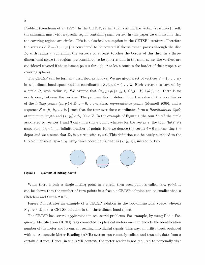
of minimum length and (xi, yi)∈Di, ∀ i∈ V . In the example of Figure 1, the tour “hits” the circle
associated to vertices 1 and 3 only in a single point, whereas for the vertex 2, the tour “hits” its
associated circle in an infinite number of points. Here we denote the vertex i= 0 representing the
depot and we assume that D0 is a circle with r0 = 0. This definition can be easily extended to the
three-dimensional space by using three coordinates, that is (xi, yi, zi), instead of two.
Figure 1 Example of hitting points
When there is only a single hitting point in a circle, then such point is called turn point. It
can be shown that the number of turn points in a feasible CETSP solution can be smaller than n
(Behdani and Smith 2013).
Figure 2 illustrates an example of a CETSP solution in the two-dimensional space, whereas
Figure 3 depicts a CETSP solution in the three-dimensional space.
The CETSP has several applications in real-world problems. For example, by using Radio Fre-
quency Identification (RFID) tags connected to physical meters one can encode the identification
number of the meter and its current reading into digital signals. This way, an utility truck equipped
with an Automatic Meter Reading (AMR) system can remotely collect and transmit data from a
certain distance. Hence, in the AMR context, the meter reader is not required to personally visit

3
Figure 2 Feasilbe solution for the CETSP in R2
Figure 3 Feasilbe solution for the CETSP in R3
each customer, but only get within a certain radius of every customer (Gulczynski et al. 2006,
Dong et al. 2007).
Unmanned Aerial Vehicles (UAVs) have been widely used for military and civil missions, espe-
cially when the presence of an human crew on board become too dangerous. As examples of
the use of UAVs we can cite Aerial Reconnaissance, Aerial Forest Fire Detection, Ship Tracking,
Supply Delivering (food, munition) to targets, Geographic Region Monitoring and Surveillance of
Pipelines. If the UAV is equipped with a sensor, the vehicle can operate successfully from a certain
distance to the target. Another example occurs when the UAV needs just to drop its cargo as
close as possible to the target locations, like in special military operations. These are all practical
applications that can be modeled as a CETSP.
Recently, Behdani and Smith (2013) pointed out that there is a lack of exact algorithms for
solving the CETSP. Moreover, Mennell et al. (2011) highlights that developing lower bounds for
the CETSP is a non-trivial task. To the best of our knowledge, the present work is the first one
to present a method that yields exact optimal solutions for the CETSP. More specifically, we
propose a simple yet effective combinatorial branch-and-bound algorithm, in which the subproblem
is based on a Second-Order Cone Programming (SOCP) formulation (Lobo et al. 1998, Farid and
Goldfarb 2003, Boyd and Vandenberghe 2004), that is capable of solving instances with up to a
thousand nodes. Moreover, our method was also designed to deal with instances both in two- and
three-dimensional spaces.
The remainder of this paper is organized as follows. Section 2 contains the related work. Section 3
describes the proposed branch-and-bound approach. Computational results are provided in Section
4. Finally, Section 5 presents the concluding remarks of this work.
2. Related work
In this section we provide a brief outline of the solution approaches proposed for solving the CETSP
and some of its related variants.
4
With a view of obtaining near-optimal solutions, several heuristics have been developed for the
CETSP. Gulczynski et al. (2006) and Dong et al. (2007) proposed several heuristic methods for
the case where all regions discs have the same radius. Their methods are based on the concept of
supernodes. A feasible supernode set S is defined as the set of points in R2, including the depot,
such that each vertex vi ∈ V , i= 1, ..., n, is within r units of at least one point S. The heuristics
were based on three distinct phases: (i) generation of the supernode set; (ii) construction of the
tour over the supernode set; and (iii) improvement of the tour by moving the supernodes. Although
the heuristics share the same main structure, the procedures adopted in each phase differ from
each other.
Yuan et al. (2007) dealt with the Optimal Robot Routing Problem (ORRP) as a TSPN where
the compact sets covering the vertices are disjoint discs with a given radius. The ORRP consists in
designing the optimal route of a mobile robot operating in a wireless sensor network in such a way
that the robot can collect data from all sensors while minimizing the total distance traveled. Hence,
this problem may be cast as a particular CETSP instance where the discs representing the action
area are all disjoint. The authors proposed a two-phase algorithm for the TSPN, by decomposing
the TSPN into a combinatorial problem and a continuous optimization problem.The former aims
to find a near-optimal solution for the TSP over the original vertices, whereas the latter is based
on an Evolutionary Algorithm that applies search space reduction techniques to find the hitting
points.
On the bases of preliminary results in Mennell (2009), Mennell et al. (2011) put forward a Steiner
Zone Heuristic based on three phases. The first one is the so-called Graph Reduction, where the
total number of vertices is reduced to a smaller number of Steiner Zones. The second one is the
Tour Finding, where a TSP tour is built over supernodes selected from each Steiner Zone. In the
last phase, denoted as Tour Improvement, exact and heuristic approaches are applied to shorten
the tour length.
Behdani and Smith (2013) proposed two different partitioning schemes to approximate the con-
tinuous covering regions. One of them is the so-called grid-based discretization, which approximates
arbitrary covering regions by rectangles. The other one is the so-called arc-based partitioning
scheme, first intended for circular covering regions, which discretizes the border of the circles
into possible hitting points. Moreover, the authors devised a Mixed Integer Programming (MIP)
approach, based on three mathematical formulations and on Benders decomposition, that was
capable of finding tight lower and upper bounds for instances with up to 21 nodes. The main
characteristic of this approach is that the more the partitioning scheme approximates the circu-
lar regions the more solutions converge to the actual optimal solution. On the other hand, high
partitioning levels make the method prohibitively expensive in terms of computing time.

5
More recently, Ha et al. (2013) studied a CETSP variant called Close Enough Arc Routing
Problem (CEARP). In the CEARP there is a predifined directed graph G = (V,A), where V =
{v0, v1, . . . , vn−1} is the set of vertices and A = {(vi, vj) | vi, vj ∈ V } is the set of arcs connecting
this vertices, and another set of vertices in R2, representing the customers and denoted by W =
{w1,w2, . . . ,wl}, that must be covered. The CEARP consists in finding a minimum-cost cycle over
the graph G such that every customer in W is covered, i.e., lies within a certain distance from
any arc of the cycle. This problems fits exactly in the AMR context, and it was originally called
CETSP over a street network by Shuttleworth et al. (2008), since in their approach the arcs of the
graph are associated to streets.
3. Branch-and-Bound algorithm
This section presents a complete description of the proposed combinatorial branch-and-bound
algorithm for the CETSP.
In summary, the method is as follows. Each branch-and-bound node is associated to an optimal
partial tour that needs to visit only a given subset of vertices in a particular order. At the root node,
the algorithm chooses three vertices in order to generate an initial sequence (see Section 3.2). Since
there are only three vertices involved in this sequence and costs are symmetric, their order will
not affect the solution. Therefore, this partial tour is a valid relaxation of the main problem. The
problem of choosing the exact coordinates of the tour to be visited, given a predefined sequence,
can be formulated as a Second Order Cone Programming (SOCP) problem (see Section 3.1). If the
associated solution is feasible (see Section 3.3), i.e., all customers are covered, then this solution
is optimal and the problem is solved. Otherwise, the algorithm branches into three subproblems,
where in each of them, a vertex that does not belong to the tour is inserted in a different position
(see Section 3.4). A node is pruned if its cost is greater than or equal to the best known upper
bound or if its associated solution is feasible. Otherwise, a branching is performed over this node
using the same rationale applied in the root node.
Figure 4 shows an example of the execution of the method for an instance involving 7 vertices.
The set of uncovered vertices is represented by a list alongside its correspondent node, whereas
the bold numbers represent the chosen vertices to be inserted. In this case, the relaxed solution
found at the root node was 0 → 3 → 6 → 0. Next, the vertex 1 was selected to be inserted in
every possible position, thus resulting in three child nodes. When inserting vertex 1 in the first or
in the second position of the tour it can be verified that vertex 4 is covered, but the same does not
happen when vertex 1 is inserted in the third position because vertex 4 still remains uncovered.
Branchings are then performed as long as they are necessary. This particular example depicts a
possible branch-and-bound tree associated to this 7-vertices instance. Prunings by bound were

6
not considerded for the sake of simplicity. As indicated in the figure, the optimal solution of this
instance is 0 → 3 → 1 → 6 → 5 → 0.
Figure 4 Example of the proposed branch-and-bound algorithm for an instance with 7 vertices
It can be noticed that the maximum number of nodes in a certain level l of the branch-and-
bound tree is given by (l+2)!
2. Moreover, in the worst case, the total number of nodes corresponds
to∑n
l=0(l+2)!
2=O(n+2)!.
3.1. Second-Order Cone Formulation
In this section we provide a mathematical formulation, based on SOCP, for solving the branch-
and-bound subproblems. This formulation has been initially proposed by Mennell (2009) for the
Touring Steiner Zones Problem when the sequence of visits is given.
Let S = {i0, . . . , iq}, q < n, be any partial sequence found during the execution of the branch-
and-bound algorithm. The subproblems of the branch-and-bound consist in finding the values of
the hitting points coordinates (xik , yik), k = 0, . . . , q, such that the length of the partial tour is
minimized. Let us assume that i−1 = iq. The formulation is as follows.
min
q∑
k=0
zk (1)
s.t. wk = xik−1−xik , k= 0, . . . , q (2)
uk = yik−1− yik , k= 0, . . . , q (3)
sk = xk −xk, k= 0, . . . , q (4)

7
tk = yk − yk, k= 0, . . . , q (5)
z2k ≥w2k +u2
k, k= 0, . . . , q (6)
s2k + t2k ≤ r2k, k= 0, . . . , q (7)
zk ≥ 0;wk, uk, sk, tk free k= 0, . . . , q (8)
xi, yi free i= 0, . . . , q (9)
In this SOCP formulation the objective function (1) is linear. The variable zk, k= 0, . . . , q, repre-
sents the distance between subsequent vertices ik−1 and ik in the partial sequence S. The auxiliary
variables w, u, s and t are defined in the linear constraints (2–5). They represent differences of coor-
dinates used to calculate Euclidean distances. The Second-Order Cone (SOC) constraints (6) define
the length of the edge connecting the subsequent customers from the sequence S. The quadratic
constraints (7) ensure that the hitting points will lie within their respective customers’ covering
circles. The expressions (8) and (9) are bounding constraints over the variables.
It is known that SOCP problems can be solved in polynomial time (Andersen et al. 2003).
Furthermore, some well-known optimization softwares are also now capable of addressing this
important class of problems.
3.2. Root relaxation
This section explains how the algorithm determines the initial sequence, i.e., the one generated at
the root node.
The three vertices from the initial sequence is selected as follows. The first vertex to be selected
is the depot. In the CETSP instances proposed in the literature the radius of the depot is assumed
to be zero. The next vertex to be chosen is the one that is most distant from the depot. The third
vertex to be inserted is the one that leads to the largest lower bound value. More specifically, the
algorithm solves a SOCP problem for all remaining candidates and selects the vertex associated to
the sequence that yields the best relaxation.
Figure 5 illustrates an example involving 7 vertices. It can be observed that the depot (vertex 0)
is the first vertex to be selected to be part of the sequence, followed by vertex 6 (the most distant
from 0), and by vertex 3, whose insertion criterion is the one just mentioned above.
3.3. Checking feasibility
In this section we explain the procedure developed for checking if a certain branch-and-bound
subproblem solution is feasible or not for the CETSP.
Let V be a set of uncovered vertices and let di be the distance between a vertex i ∈ V and the
edge of a subproblem solution that is nearest to i. Suppose that c and p1p2 are an arbitrary vertex

8
Figure 5 Example of the procedure to find a valid root relaxation
and an arbitrary edge of a partial solution. We are interested in determining the coordinates of a
point p∈ p1p2 that minimizes the distance between p1p2 and c.
The minimum distance d between c and p1p2 is computed by solving the optimization problem
defined by Equation (10):
d= min0≤θ≤1
‖(1− θ)p1 + θp2 − c‖ (10)
whose analytical solution to the unconstrained problem is given by θ∗ =− (p2−p1)⊤(p1−c)
‖p2−p1‖2. Therefore,
the minimum distance can be computed by Equation (11):
d=
‖p1 − c‖, if θ∗ ≤ 0
‖p− c‖, if 0< θ∗ < 1, where p= (1− θ∗)p1 + θ∗p2
‖p2 − c‖, if θ∗ ≥ 1
(11)
In order to check the feasibility of a subproblem solution one must compute the value of d for
every vertex, i.e. not in the current subsequence, and for every existent edge in this partial solution,
compare with the corresponding disk radius. If d is not greater than such radius, than the vertex
is considered covered. If the number of vertices is given by u and the number of edges is given by
v then this verification takes O(uv) operations. Note that this approach allows for dealing with
instances in R2 or R3.
Figure 6 Example involving an edge and three uncovered vertices of a partial CETSP solution

9
Figure 6 shows an example for three vertices and one edge. For vertex 1, θ∗ < 0, thus the minimum
distance between c and p1p2 is equal to the distance between c and p1. For vertex 2, 0< θ∗ < 1, thus
the minimum distance between c and p1p2 is equal to the distance between c and p. Finally, for
vertex 3, θ∗ > 1, thus the minimum distance between c and p1p2 is equal to the distance between
c and p2
3.4. Branching rules
In this section we describe the two branching criteria used to select a vertex to be inserted in
a partial solution associated to a node of the branch-and-bound tree. The adequate criterion is
automatically chosen based on the radii of the instances.
If all vertices have the same radius, the method proceed as follows. The algorithm first computes
the value of dk for every k ∈ V . Next, the maximum value among all dk is determined, that is,
maxk∈V {dk}, and the corresponding vertex k is selected to be inserted in the partial solution.
Figure 7 depicts an example of how the vertex selection is performed. In this case, we are given a
partial solution 0 → 3 → 6 → 0. Note that vertex 4 is covered, but vertices 1 and 2 are not, thus
V = {1,2}. It can be seen that d1 > d2. Hence, vertex 1 is the one associated to maxk∈V {dk}.
Figure 7 Illustration of the branching rule used when all vertices have the same radius
If the vertices have different radii, the following schemed is used. At First, for all vertices k ∈ V ,
the algorithm computes an estimative, given by γk, of how much the lower bound would increase
if the vertex k were inserted between its closest neighbors in the sequence. In order to estimate
γk, the procedure first calculates the coordinates of the point pk on the border of the disk Dk
that minimizes the distance between this point and its nearest edge p1p2 on the sequence. Hence,
γk can be computed as γk = ek1 + ek2 − eij, where ek1 is the distance between pk and p1, ek2 is the
distance between pk and p2 and eij is the length of the edge p1p2. Figure 8 shows an example of
this procedure, where V = {1,2}. Therefore γ1 = e11 + e12 − e34 and γ2 = e21 + e22 − e40. Suppose that
γ2 > γ1, as the figure suggest. Therefore, following the second branching rule, the vertex 2 is the
one to be inserted in the sequence.

10
Figure 8 Illustration of the branching rule used when the vertices have different radii
4. Computational experiments
The branch-and-bound algorithm was coded in C++ and the tests were carried out in an Intel
Core i7 with 3.40 GHz and 16 GB of RAM running under Linux Mint 13. The SOCPs were solved
using CPLEX 12.4. Only a single thread was used in our experiments. The 3D illustrations were
generated using a MATLAB routine called BUBBLEPLOT3 (Bodin 2009).
We performed a series of experiments to choose the most interesting branching strategy to be
adopted. Tests were carried out using the following strategies: depth-first search, breadth-first
search and best-first search. The results revealed that the best-first search turned out to be the
most suitable strategy to be applied in our algorithm.
The proposed algorithm was tested in 824 instances that were suggested by Mennell (2009) and
Behdani and Smith (2013). The difficulty of each instance is associated with the notion of overlap
ratio, given by Mennell (2009), which is defined as the ratio between the mean of the radii of all
vertices and the largest side (lmax) of the rectangle that involve all vertices and their radii, i.e.,
overlap ratio=(∑
n
i=0ri)/n
lmax.
Mennell (2009) presents the following classifications for his instances. Six problems whose names
start with team, plus the instance bonus1000 were denoted Team Problems. Those starting with
rotatingDiamonds, bubbles, concentricCircles, plus the instance chaoSigleDep were gathered in the
subset calledGeometric Problems. Finally, the instances d493, dsj1000, kroD100, lin318, pcb442,
rat195 and rd400 were generated from the TSPLIB and they were called TSPLIB Problems.
The instances of the groups Team Problems and Geometric Problems were generated with ri =
r, i = 0, . . . , n, and different overlap ratios that were not specified. The instances of the group
TSPLIB Problems were generated with radii of three different sizes, i.e., with three overlap ratios,
namely: 0.02, 0.10 and 0.30. Only the instances of the groups Team Problems and TSPLIB Problems
have 3D versions. Mennell (2009) also provided two groups of instances denoted Team Random
Radius Problems and TSPLIB Random Radius Problems, with 2D and 3D versions, with
radii generated at random in such a way that ri 6= rj,∀i, j ∈ V .
Behdani and Smith (2013) provided 240 2D test-problems with 7, 9, 11, 13, 15, 17, 19 and 21
vertices. These instances were generated as follows. The position (xi, yi), i∈ V , of each vertex and

11
the depot i0 were selected at random in a limited space of 16 units of length and 10 units if width.
The coverage area of all vertices was defined as a circumference with radius r. In their experiments,
the authors used three radii, namely: 0.25, 0.50 and 1.00, thus obtaining three distinct groups with
overlap ratios 0.015, 0.030 and 0.060, respectively.
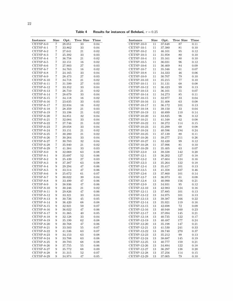
4.1. Results found for the small instances of Behdani and Smith (2013)
Table 1 shows a summary of the results found for the instances of Behdani and Smith (2013). In
this table, Group denotes the 8 groups of instances divided into three different subgroups (overlap
ratios = 0.015, 0.030, 0.060), Group Size shows the number of instances of each group, #Opt.
indicates the number of optimal solutions obtained for each group, Tree Size corresponds to the
average tree size and Avg. Time is the average time, in seconds.
Table 1 Summary results for instances of Behdani
Group Group Size #Opt. Avg. Tree Size Avg. Time
r = 0.25 and overlap = 0.0156
CETSP-06 30 30 26 0.029
CETSP-08 30 30 51 0.062
CETSP-10 30 30 86 0.107
CETSP-12 30 30 139 0.189
CETSP-14 30 30 219 0.308
CETSP-16 30 30 443 0.673
CETSP-18 30 30 544 0.839
CETSP-20 30 30 1016 1.656
r = 0.50 and overlap = 0.0313
CETSP-06 30 30 19 0.020
CETSP-08 30 30 39 0.047
CETSP-10 30 30 66 0.085
CETSP-12 30 30 92 0.125
CETSP-14 30 30 144 0.204
CETSP-16 30 30 222 0.334
CETSP-18 30 30 331 0.525
CETSP-20 30 30 437 0.719
r = 1.0 and overlap = 0.0625
CETSP-06 30 30 13 0.017
CETSP-08 30 30 23 0.030
CETSP-10 30 30 38 0.049
CETSP-12 30 30 51 0.066
CETSP-14 30 30 71 0.100
CETSP-16 30 30 95 0.144
CETSP-18 30 30 117 0.176
CETSP-20 30 30 163 0.261
From Table 1, it can be observed the all instances were solved to optimality in a matter of
seconds, as opposed to the method of Behdani and Smith (2013) whose lower/upper bounds were
obtained in much higher computing time.
The complete results obtained by our branch-and-bound algorithm for the instances of Behdani
and Smith (2013) can be found in Appendix.
12
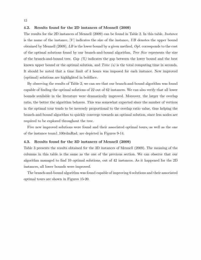
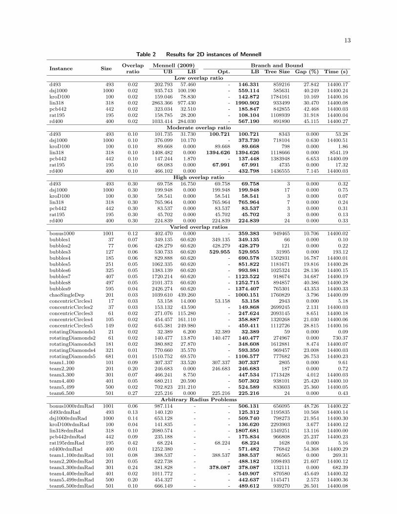
4.2. Results found for the 2D instances of Mennell (2009)
The results for the 2D instances of Mennell (2009) can be found in Table 2. In this table, Instance
is the name of the instance, |V | indicates the size of the instance, UB denotes the upper bound
obtained by Mennell (2009), LB is the lower bound by a given method, Opt. corresponds to the cost
of the optimal solutions found by our branch-and-bound algorithm, Tree Size represents the size
of the branch-and-bound tree, Gap (%) indicates the gap between the lower bound and the best
known upper bound or the optimal solution, and Time (s) is the total computing time in seconds.
It should be noted that a time limit of 4 hours was imposed for each instance. New improved
(optimal) solutions are highlighted in boldface.
By observing the results of Table 2, we can see that our branch-and-bound algorithm was found
capable of finding the optimal solutions of 22 out of 62 instances. We can also verify that all lower
bounds available in the literature were dramatically improved. Moreover, the larger the overlap
ratio, the better the algorithm behaves. This was somewhat expected since the number of vertices
in the optimal tour tends to be inversely proportional to the overlap ratio value, thus helping the
branch-and-bound algorithm to quickly converge towards an optimal solution, since less nodes are
required to be explored throughout the tree.
Five new improved solutions were found and their associated optimal tours, as well as the one
of the instance team1 100rdmRad, are depicted in Figures 9-14.
4.3. Results found for the 3D instances of Mennell (2009)
Table 3 presents the results obtained for the 3D instances of Mennell (2009). The meaning of the
columns in this table is the same as the one of the previous section. We can observe that our
algorithm managed to find 10 optimal solutions, out of 42 instances. As it happened for the 2D
instances, all lower bounds were improved.
The branch-and-bound algorithm was found capable of improving 6 solutions and their associated
optimal tours are shown in Figures 15-20.
13
Table 2 Results for 2D instances of Mennell
Instance SizeOverlapratio
Mennell (2009) Branch and BoundUB LB Opt. LB Tree Size Gap (%) Time (s)
Low overlap ratiod493 493 0.02 202.793 57.460 - 146.331 859216 27.842 14400.17
dsj1000 1000 0.02 935.743 100.190 - 559.114 585631 40.249 14400.24
kroD100 100 0.02 159.046 78.830 - 142.872 1784161 10.169 14400.16
lin318 318 0.02 2863.366 977.430 - 1990.902 933499 30.470 14400.08
pcb442 442 0.02 323.034 32.510 - 185.847 842855 42.468 14400.03
rat195 195 0.02 158.785 28.200 - 108.104 1108939 31.918 14400.04
rd400 400 0.02 1033.414 284.030 - 567.190 891890 45.115 14400.27
Moderate overlap ratiod493 493 0.10 101.735 31.730 100.721 100.721 8343 0.000 53.28
dsj1000 1000 0.10 376.099 10.170 - 373.730 718104 0.630 14400.51
kroD100 100 0.10 89.668 0.000 89.668 89.668 798 0.000 1.86
lin318 318 0.10 1408.482 0.000 1394.626 1394.626 1118666 0.000 8541.19
pcb442 442 0.10 147.244 1.870 - 137.448 1383948 6.653 14400.09
rat195 195 0.10 68.083 0.000 67.991 67.991 4735 0.000 17.32
rd400 400 0.10 466.102 0.000 - 432.798 1436555 7.145 14400.03
High overlap ratiod493 493 0.30 69.758 16.750 69.758 69.758 3 0.000 0.32
dsj1000 1000 0.30 199.948 0.000 199.948 199.948 17 0.000 0.75
kroD100 100 0.30 58.541 0.000 58.541 58.541 3 0.000 0.07
lin318 318 0.30 765.964 0.000 765.964 765.964 7 0.000 0.24
pcb442 442 0.30 83.537 0.000 83.537 83.537 3 0.000 0.31
rat195 195 0.30 45.702 0.000 45.702 45.702 3 0.000 0.13
rd400 400 0.30 224.839 0.000 224.839 224.839 24 0.000 0.33
Varied overlap ratiosbonus1000 1001 0.12 402.470 0.000 - 359.383 949465 10.706 14400.02
bubbles1 37 0.07 349.135 60.620 349.135 349.135 66 0.000 0.10
bubbles2 77 0.06 428.279 60.620 428.279 428.279 121 0.000 0.22
bubbles3 127 0.06 530.733 60.620 529.955 529.955 31995 0.000 193.12
bubbles4 185 0.06 829.888 60.620 - 690.578 1502931 16.787 14400.01
bubbles5 251 0.05 1062.335 60.620 - 851.822 1181671 19.816 14400.28
bubbles6 325 0.05 1383.139 60.620 - 993.981 1025324 28.136 14400.15
bubbles7 407 0.05 1720.214 60.620 - 1123.522 918674 34.687 14400.19
bubbles8 497 0.05 2101.373 60.620 - 1252.715 894857 40.386 14400.28
bubbles9 595 0.04 2426.274 60.620 - 1374.407 765301 43.353 14400.33
chaoSingleDep 201 0.03 1039.610 439.260 - 1000.151 1760829 3.796 14400.09
concentricCircles1 17 0.03 53.158 14.000 53.158 53.158 2943 0.000 5.18
concentricCircles2 37 0.03 153.132 43.590 - 149.868 2699245 2.131 14400.03
concentricCircles3 61 0.02 271.076 115.280 - 247.624 2093145 8.651 14400.18
concentricCircles4 105 0.02 454.457 161.110 - 358.887 1320268 21.030 14400.06
concentricCircles5 149 0.02 645.381 249.980 - 459.411 1112726 28.815 14400.16
rotatingDiamonds1 21 0.02 32.389 6.200 32.389 32.389 59 0.000 0.09
rotatingDiamonds2 61 0.02 140.477 13.870 140.477 140.477 274967 0.000 730.37
rotatingDiamonds3 181 0.02 380.882 27.870 - 348.608 1612881 8.474 14400.07
rotatingDiamonds4 321 0.01 770.660 35.570 - 593.350 969457 23.008 14400.03
rotatingDiamonds5 681 0.01 1510.752 69.570 - 1106.577 777682 26.753 14400.23
team1 100 101 0.09 307.337 33.520 307.337 307.337 2805 0.000 9.61
team2 200 201 0.20 246.683 0.000 246.683 246.683 187 0.000 0.72
team3 300 301 0.07 466.241 8.750 - 447.534 1713428 4.012 14400.03
team4 400 401 0.05 680.211 20.590 - 507.302 938101 25.420 14400.10
team5 499 500 0.02 702.823 231.210 - 524.589 833603 25.360 14400.05
team6 500 501 0.27 225.216 0.000 225.216 225.216 24 0.000 0.43
Arbitrary Radius Problemsbonus1000rdmRad 1001 0.06 987.114 - - 506.131 656095 48.726 14400.22
d493rdmRad 493 0.13 140.120 - - 125.312 1195835 10.568 14400.14
dsj1000rdmRad 1000 0.14 653.128 - - 509.740 798273 21.954 14400.30
kroD100rdmRad 100 0.04 141.835 - - 136.620 2293903 3.677 14400.12
lin318rdmRad 318 0.10 2080.574 - - 1807.681 1349251 13.116 14400.00
pcb442rdmRad 442 0.09 235.188 - - 175.834 966808 25.237 14400.23
rat195rdmRad 195 0.42 68.224 - 68.224 68.224 1628 0.000 5.16
rd400rdmRad 400 0.01 1252.380 - - 571.482 776842 54.368 14400.29
team1 100rdmRad 101 0.08 388.537 - 388.537 388.537 86565 0.000 269.31
team2 200rdmRad 201 0.05 622.738 - - 488.182 1098493 21.607 14400.12
team3 300rdmRad 301 0.24 381.828 - 378.087 378.087 132111 0.000 682.39
team4 400rdmRad 401 0.02 1011.772 - - 549.907 870580 45.649 14400.32
team5 499rdmRad 500 0.20 454.327 - - 442.637 1145471 2.573 14400.36
team6 500rdmRad 501 0.10 666.149 - - 489.612 939270 26.501 14400.08

14
Figure 9 Solution for kroD100, Equal radius, 2D, Size = 100, Lenght = 89.668
Figure 10 Solution for team1 100rdmRad, Arbitrary radius, 2D, Size = 101, Lenght = 388.537
Figure 11 Solution for rat195, Equal radius, 2D, Size = 195, Lenght = 67.991

15
Figure 12 Solution for team3 300rdmRad, Arbitrary radius, 2D, Size = 301, Lenght = 378.087
Figure 13 Solution for lin318, Equal radius, 2D, Size = 318, Lenght = 1394.626
Figure 14 Solution for d493, Equal radius, 2D, Size = 493, Lenght = 100.721

16
Table 3 Results for 3D instances of Mennell
Instance SizeOverlapratio
Mennell (2009) Branch and BoundUB LB Opt. LB Tree Size Gap (%) Time (s)
Low overlap ratiod493 493 0.01 1353.137 - - 469.783 642868 65.282 14400.01
dsj1000 1000 0.02 3147.865 - - 751.510 494579 76.126 14400.05
kroD100 100 0.02 202.021 - - 148.231 1183277 26.626 14400.12
lin318 318 0.02 3044.270 - - 1994.372 934859 34.488 14400.14
pcb442 442 0.02 404.490 - - 186.381 725462 53.922 14400.18
rat195 195 0.02 291.258 - - 126.493 978598 56.570 14400.06
rd400 400 0.02 3218.198 - - 868.188 753967 73.023 14400.12
Moderate overlap ratiod493 493 0.03 665.056 - - 421.164 827584 36.672 14400.18
dsj1000 1000 0.10 1021.252 - - 602.987 644546 40.956 14400.31
kroD100 100 0.10 91.669 - 91.663 91.663 2407 0.000 7.51
lin318 318 0.10 1443.427 - - 1398.254 1588841 3.130 14400.12
pcb442 442 0.10 154.810 - - 137.951 1209228 10.890 14400.13
rat195 195 0.10 112.405 - - 88.721 1325338 21.070 14400.13
rd400 400 0.10 1552.723 - - 752.423 851059 51.542 14400.24
High overlap ratiod493 493 0.08 335.592 - 325.207 325.207 5064 0.000 31.11
dsj1000 1000 0.30 270.399 - 267.751 267.751 2472 0.000 25.07
kroD100 100 0.30 58.926 - 58.926 58.926 4 0.000 0.08
lin318 318 0.30 766.831 - 766.831 766.831 8 0.000 0.24
pcb442 442 0.30 83.722 - 83.722 83.722 4 0.000 0.33
rat195 195 0.30 47.889 - 47.889 47.889 4 0.000 0.14
rd400 400 0.30 539.954 - - 450.720 507442 16.526 14400.40
Varied overlap ratiosbonus1000 1001 0.12 941.348 - - 472.559 655479 49.800 14400.35
team1 100 101 0.09 820.727 - - 690.298 1197716 15.892 14400.22
team2 200 201 0.20 283.238 - 273.383 273.383 86492 0.000 557.94
team3 300 301 0.07 1484.411 - - 762.683 930319 48.620 14400.12
team4 400 401 0.05 753.813 - - 509.803 894994 32.370 14400.30
team5 499 500 0.02 1924.527 - - 705.633 665171 63.335 14400.20
team6 500 501 0.27 236.964 - 230.923 230.923 73 0.000 0.67
Arbitrary Radius Problemsbonus1000rdmRad 1001 0.06 2689.413 - - 578.638 512678 78.485 14400.04
d493rdmRad 493 0.03 761.065 - - 438.701 858509 42.357 14400.06
dsj1000rdmRad 1000 0.14 2074.844 - - 696.289 656155 66.441 14400.05
kroD100rdmRad 100 0.04 171.568 - - 137.765 1350550 19.702 14400.13
lin318rdmRad 318 0.10 2189.426 - - 1806.783 1200921 17.477 14400.10
pcb442rdmRad 442 0.09 258.404 - - 177.231 962861 31.413 14400.09
rat195rdmRad 195 0.42 84.470 - 82.105 82.105 152636 0.000 790.53
rd400rdmRad 400 0.01 3592.601 - - 876.280 766218 75.609 14400.06
team1 100rdmRad 101 0.08 907.593 - - 726.685 1137079 19.933 14400.26
team2 200rdmRad 201 0.05 1055.948 - - 525.310 1027597 50.252 14400.20
team3 300rdmRad 301 0.24 1053.380 - - 676.184 1004637 35.808 14400.10
team4 400rdmRad 401 0.02 1276.896 - - 551.046 793139 56.845 14400.08
team5 499rdmRad 500 0.20 840.477 - - 599.741 940015 28.643 14400.28
team6 500rdmRad 501 0.10 1076.352 - - 507.122 870473 52.885 14400.12
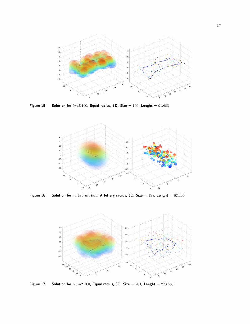
17
Figure 15 Solution for kroD100, Equal radius, 3D, Size = 100, Lenght = 91.663
Figure 16 Solution for rat195rdmRad, Arbitrary radius, 3D, Size = 195, Lenght = 82.105
Figure 17 Solution for team2 200, Equal radius, 3D, Size = 201, Lenght = 273.383

18
Figure 18 Solution for d493, Equal radius, 3D, Size = 493, Lenght = 325.207
Figure 19 Solution for team6 500, Equal radius, 3D, Size = 501, Lenght = 230.923
Figure 20 Solution for dsj1000, Equal radius, 3D, Size = 1000, Lenght = 267.751

19
5. Conclusions
This work presented a combinatorial branch-and-bound algorithm for the Close-Enough Traveling
Salesman Problem (CETSP), where the subproblems solved in each node consists of a Second
Order Cone Programming (SOCP). The proposed algorithm was tested in 824 instances available
in the literature, namely: 720 two-dimensional instances suggested by Behdani and Smith (2013);
62 two-dimensional instances generated by Mennell (2009); and 42 three-dimensional instances
developed by Mennell (2009). Our algorithm was found capable of obtaining the optimal solutions
for 752 instances, more precisely, all 720 instances of Behdani and Smith (2013), 22 two-dimensional
instances of Mennell (2009) and 10 three-dimensional instances of Mennell (2009). The lower bounds
of all remaining instances were also improved.
The proposed algorithm performed quite well particularly on those instances with larger overlap
ratios. In practical terms, these type of instances are more closely related with the technological
advance. For example, better wireless transmitters and receptors tend to increase the coverage area
of the equipments that use this type of technology, as in the case of AMR and other applications
found in the literature, i.e., the radius of each vertex is likely to increase with the development of
new technologies.
Promising avenues of research include the development of new approaches to improve the root
relaxation, especially for smaller overlap ratios where the problem becomes closer to the classical
TSP.

20
Acknowledgments
The authors thank Dr. Manuel Iori for the valuable comments that helped improving the quality of the paper
and Dr. Behdani and Dr. Smith for providing the instances generated in Behdani and Smith (2013).

21
Appendix. Optimal solution found for instances of Behdani and Smith
(2013)
22
Table 4 Results for instances of Behdani, r= 0.25
Instance Size Opt. Tree Size TimeCETSP-6-0 7 28.051 33 0.04
CETSP-6-1 7 33.862 33 0.04
CETSP-6-2 7 27.641 21 0.02
CETSP-6-3 7 25.392 33 0.03
CETSP-6-4 7 36.758 21 0.02
CETSP-6-5 7 22.151 16 0.02
CETSP-6-6 7 27.903 27 0.03
CETSP-6-7 7 34.763 16 0.02
CETSP-6-8 7 24.165 33 0.04
CETSP-6-9 7 28.473 27 0.03
CETSP-6-10 7 34.718 21 0.02
CETSP-6-11 7 31.599 27 0.03
CETSP-6-12 7 33.352 33 0.04
CETSP-6-13 7 26.710 21 0.02
CETSP-6-14 7 28.679 33 0.04
CETSP-6-15 7 34.118 16 0.02
CETSP-6-16 7 23.635 33 0.03
CETSP-6-17 7 22.834 16 0.02
CETSP-6-18 7 28.359 21 0.03
CETSP-6-19 7 33.198 21 0.02
CETSP-6-20 7 34.851 32 0.04
CETSP-6-21 7 32.084 33 0.04
CETSP-6-22 7 27.746 21 0.02
CETSP-6-23 7 29.058 33 0.04
CETSP-6-24 7 33.151 21 0.02
CETSP-6-25 7 30.280 21 0.02
CETSP-6-26 7 30.264 33 0.04
CETSP-6-27 7 30.783 32 0.04
CETSP-6-28 7 35.940 21 0.02
CETSP-6-29 7 41.384 33 0.03
CETSP-8-0 9 32.069 63 0.08
CETSP-8-1 9 35.697 52 0.06
CETSP-8-2 9 25.439 27 0.03
CETSP-8-3 9 37.387 63 0.08
CETSP-8-4 9 29.294 47 0.06
CETSP-8-5 9 33.514 47 0.06
CETSP-8-6 9 25.672 61 0.07
CETSP-8-7 9 30.022 39 0.04
CETSP-8-8 9 33.499 47 0.06
CETSP-8-9 9 38.936 47 0.06
CETSP-8-10 9 30.246 21 0.02
CETSP-8-11 9 29.826 47 0.06
CETSP-8-12 9 33.321 33 0.04
CETSP-8-13 9 30.726 45 0.05
CETSP-8-14 9 36.420 68 0.08
CETSP-8-15 9 32.921 59 0.07
CETSP-8-16 9 36.022 47 0.06
CETSP-8-17 9 31.365 40 0.05
CETSP-8-18 9 32.128 33 0.04
CETSP-8-19 9 35.199 62 0.08
CETSP-8-20 9 30.768 47 0.06
CETSP-8-21 9 33.503 55 0.07
CETSP-8-22 9 41.536 63 0.07
CETSP-8-23 9 34.153 63 0.08
CETSP-8-24 9 33.788 63 0.08
CETSP-8-25 9 39.793 68 0.08
CETSP-8-26 9 37.755 55 0.06
CETSP-8-27 9 35.772 68 0.09
CETSP-8-28 9 31.315 52 0.07
CETSP-8-29 9 34.974 47 0.05
Instance Size Opt. Tree Size TimeCETSP-10-0 11 37.648 87 0.11
CETSP-10-1 11 37.380 81 0.10
CETSP-10-2 11 46.101 95 0.12
CETSP-10-3 11 31.958 80 0.10
CETSP-10-4 11 35.161 80 0.10
CETSP-10-5 11 36.031 96 0.12
CETSP-10-6 11 36.469 84 0.09
CETSP-10-7 11 35.346 61 0.07
CETSP-10-8 11 34.333 46 0.06
CETSP-10-9 11 30.707 79 0.10
CETSP-10-10 11 35.215 77 0.10
CETSP-10-11 11 31.131 68 0.08
CETSP-10-12 11 36.423 99 0.13
CETSP-10-13 11 36.101 55 0.07
CETSP-10-14 11 34.273 85 0.11
CETSP-10-15 11 32.977 33 0.04
CETSP-10-16 11 31.408 63 0.08
CETSP-10-17 11 36.172 101 0.13
CETSP-10-18 11 39.150 33 0.04
CETSP-10-19 11 40.899 110 0.14
CETSP-10-20 11 33.825 96 0.12
CETSP-10-21 11 41.348 62 0.08
CETSP-10-22 11 38.272 114 0.15
CETSP-10-23 11 35.299 68 0.08
CETSP-10-24 11 40.596 194 0.24
CETSP-10-25 11 37.139 88 0.11
CETSP-10-26 11 39.277 211 0.26
CETSP-10-27 11 32.420 99 0.12
CETSP-10-28 11 37.996 81 0.10
CETSP-10-29 11 35.405 63 0.07
CETSP-12-0 13 39.338 142 0.20
CETSP-12-1 13 36.202 127 0.18
CETSP-12-2 13 47.604 124 0.16
CETSP-12-3 13 35.264 122 0.18
CETSP-12-4 13 35.417 101 0.13
CETSP-12-5 13 41.358 337 0.46
CETSP-12-6 13 37.860 101 0.14
CETSP-12-7 13 36.973 61 0.08
CETSP-12-8 13 40.990 156 0.21
CETSP-12-9 13 34.931 95 0.12
CETSP-12-10 13 42.983 124 0.16
CETSP-12-11 13 37.885 101 0.13
CETSP-12-12 13 34.975 101 0.13
CETSP-12-13 13 39.387 166 0.22
CETSP-12-14 13 35.921 119 0.16
CETSP-12-15 13 42.698 72 0.09
CETSP-12-16 13 40.948 160 0.23
CETSP-12-17 13 37.094 145 0.21
CETSP-12-18 13 40.735 122 0.17
CETSP-12-19 13 40.487 177 0.24
CETSP-12-20 13 35.198 147 0.21
CETSP-12-21 13 41.530 241 0.33
CETSP-12-22 13 39.740 270 0.37
CETSP-12-23 13 35.212 99 0.13
CETSP-12-24 13 38.687 145 0.19
CETSP-12-25 13 40.777 159 0.21
CETSP-12-26 13 34.894 122 0.18
CETSP-12-27 13 36.297 138 0.20
CETSP-12-28 13 37.256 114 0.15
CETSP-12-29 13 37.005 79 0.10

23
Table 5 Results for instances of Behdani, r= 0.25
Instance Size Opt. Tree Size TimeCETSP-14-0 15 40.445 209 0.32
CETSP-14-1 15 41.751 231 0.31
CETSP-14-2 15 40.154 388 0.62
CETSP-14-3 15 36.239 123 0.18
CETSP-14-4 15 41.032 454 0.57
CETSP-14-5 15 36.336 166 0.25
CETSP-14-6 15 36.549 93 0.12
CETSP-14-7 15 42.216 210 0.29
CETSP-14-8 15 37.416 168 0.23
CETSP-14-9 15 37.945 99 0.13
CETSP-14-10 15 37.478 170 0.25
CETSP-14-11 15 39.180 200 0.28
CETSP-14-12 15 37.982 214 0.33
CETSP-14-13 15 44.277 137 0.19
CETSP-14-14 15 43.238 210 0.33
CETSP-14-15 15 41.829 165 0.26
CETSP-14-16 15 45.761 226 0.30
CETSP-14-17 15 36.990 461 0.64
CETSP-14-18 15 42.912 563 0.79
CETSP-14-19 15 40.263 421 0.60
CETSP-14-20 15 36.329 147 0.20
CETSP-14-21 15 38.699 146 0.19
CETSP-14-22 15 42.718 307 0.42
CETSP-14-23 15 40.349 102 0.14
CETSP-14-24 15 41.446 137 0.18
CETSP-14-25 15 37.190 100 0.14
CETSP-14-26 15 43.857 192 0.28
CETSP-14-27 15 38.837 215 0.30
CETSP-14-28 15 39.600 186 0.22
CETSP-14-29 15 35.514 118 0.17
CETSP-16-0 17 40.875 261 0.40
CETSP-16-1 17 46.802 140 0.20
CETSP-16-2 17 38.612 286 0.44
CETSP-16-3 17 43.401 213 0.32
CETSP-16-4 17 39.596 344 0.57
CETSP-16-5 17 38.984 186 0.27
CETSP-16-6 17 43.818 432 0.65
CETSP-16-7 17 40.548 588 0.83
CETSP-16-8 17 39.123 196 0.31
CETSP-16-9 17 35.423 170 0.22
CETSP-16-10 17 37.432 236 0.36
CETSP-16-11 17 41.860 336 0.54
CETSP-16-12 17 52.277 374 0.55
CETSP-16-13 17 42.703 198 0.32
CETSP-16-14 17 46.434 288 0.39
CETSP-16-15 17 41.872 1517 2.47
CETSP-16-16 17 41.846 831 1.30
CETSP-16-17 17 39.106 404 0.64
CETSP-16-18 17 45.459 962 1.35
CETSP-16-19 17 43.594 546 0.78
CETSP-16-20 17 46.199 340 0.48
CETSP-16-21 17 41.393 171 0.25
CETSP-16-22 17 38.608 165 0.26
CETSP-16-23 17 43.711 344 0.55
CETSP-16-24 17 40.266 2007 3.00
CETSP-16-25 17 40.601 481 0.76
CETSP-16-26 17 41.155 247 0.36
CETSP-16-27 17 45.308 320 0.51
CETSP-16-28 17 44.838 306 0.44
CETSP-16-29 17 43.588 397 0.66
Instance Size Opt. Tree Size TimeCETSP-18-0 19 41.322 362 0.60
CETSP-18-1 19 48.079 250 0.35
CETSP-18-2 19 41.234 445 0.72
CETSP-18-3 19 44.681 1259 1.94
CETSP-18-4 19 44.842 238 0.40
CETSP-18-5 19 40.794 211 0.33
CETSP-18-6 19 40.294 798 1.10
CETSP-18-7 19 38.894 173 0.28
CETSP-18-8 19 35.898 140 0.19
CETSP-18-9 19 37.798 264 0.44
CETSP-18-10 19 44.962 295 0.46
CETSP-18-11 19 50.117 722 1.18
CETSP-18-12 19 44.023 354 0.55
CETSP-18-13 19 43.899 507 0.78
CETSP-18-14 19 45.635 1331 2.05
CETSP-18-15 19 42.191 475 0.69
CETSP-18-16 19 45.936 907 1.36
CETSP-18-17 19 45.855 1068 1.66
CETSP-18-18 19 46.274 319 0.48
CETSP-18-19 19 43.434 290 0.44
CETSP-18-20 19 43.548 270 0.38
CETSP-18-21 19 38.735 1246 1.96
CETSP-18-22 19 40.608 291 0.40
CETSP-18-23 19 41.802 284 0.39
CETSP-18-24 19 47.271 1011 1.66
CETSP-18-25 19 45.342 272 0.44
CETSP-18-26 19 47.429 404 0.65
CETSP-18-27 19 43.228 381 0.65
CETSP-18-28 19 42.901 684 1.11
CETSP-18-29 19 46.983 1066 1.53
CETSP-20-0 21 41.663 480 0.84
CETSP-20-1 21 48.582 808 1.30
CETSP-20-2 21 39.706 318 0.56
CETSP-20-3 21 52.071 3147 5.32
CETSP-20-4 21 42.449 541 0.88
CETSP-20-5 21 46.030 479 0.72
CETSP-20-6 21 47.124 996 1.52
CETSP-20-7 21 42.608 313 0.54
CETSP-20-8 21 41.654 712 1.12
CETSP-20-9 21 46.386 419 0.70
CETSP-20-10 21 46.776 1393 2.30
CETSP-20-11 21 46.903 497 0.86
CETSP-20-12 21 43.134 1173 2.01
CETSP-20-13 21 45.156 1678 2.77
CETSP-20-14 21 43.382 930 1.41
CETSP-20-15 21 43.001 541 0.88
CETSP-20-16 21 46.982 917 1.45
CETSP-20-17 21 44.101 356 0.54
CETSP-20-18 21 46.090 397 0.66
CETSP-20-19 21 44.669 3832 6.12
CETSP-20-20 21 47.551 2155 3.52
CETSP-20-21 21 43.062 392 0.62
CETSP-20-22 21 46.051 740 1.22
CETSP-20-23 21 48.816 2133 3.60
CETSP-20-24 21 47.472 413 0.73
CETSP-20-25 21 46.423 1691 2.65
CETSP-20-26 21 48.101 955 1.44
CETSP-20-27 21 45.339 472 0.75
CETSP-20-28 21 48.392 1365 2.29
CETSP-20-29 21 42.662 245 0.37

24
Table 6 Results for instances of Behdani, r= 0.50
Instance Size Opt. Tree Size TimeCETSP-6-0 7 27.164 21 0.02
CETSP-6-1 7 32.438 16 0.02
CETSP-6-2 7 26.227 16 0.02
CETSP-6-3 7 23.935 21 0.02
CETSP-6-4 7 35.406 21 0.02
CETSP-6-5 7 20.845 21 0.02
CETSP-6-6 7 26.733 11 0.01
CETSP-6-7 7 33.762 7 0.01
CETSP-6-8 7 23.139 16 0.02
CETSP-6-9 7 26.858 21 0.02
CETSP-6-10 7 33.643 3 0.00
CETSP-6-11 7 30.132 27 0.03
CETSP-6-12 7 31.772 21 0.02
CETSP-6-13 7 25.305 21 0.02
CETSP-6-14 7 27.151 16 0.02
CETSP-6-15 7 33.025 16 0.02
CETSP-6-16 7 22.020 16 0.02
CETSP-6-17 7 21.703 11 0.01
CETSP-6-18 7 27.068 21 0.02
CETSP-6-19 7 32.157 21 0.02
CETSP-6-20 7 33.252 32 0.04
CETSP-6-21 7 30.580 33 0.04
CETSP-6-22 7 26.557 21 0.02
CETSP-6-23 7 28.093 21 0.02
CETSP-6-24 7 31.733 21 0.02
CETSP-6-25 7 29.335 7 0.01
CETSP-6-26 7 28.663 21 0.02
CETSP-6-27 7 28.979 32 0.03
CETSP-6-28 7 34.603 11 0.01
CETSP-6-29 7 39.621 21 0.02
CETSP-8-0 9 30.944 16 0.02
CETSP-8-1 9 34.073 47 0.06
CETSP-8-2 9 24.006 33 0.04
CETSP-8-3 9 35.591 47 0.06
CETSP-8-4 9 27.767 47 0.06
CETSP-8-5 9 31.987 27 0.03
CETSP-8-6 9 24.419 39 0.05
CETSP-8-7 9 27.828 40 0.06
CETSP-8-8 9 31.971 21 0.03
CETSP-8-9 9 37.380 33 0.04
CETSP-8-10 9 28.967 21 0.02
CETSP-8-11 9 28.288 47 0.06
CETSP-8-12 9 31.521 33 0.04
CETSP-8-13 9 28.872 33 0.04
CETSP-8-14 9 34.467 68 0.08
CETSP-8-15 9 31.669 47 0.06
CETSP-8-16 9 34.394 33 0.04
CETSP-8-17 9 30.064 21 0.02
CETSP-8-18 9 30.813 33 0.04
CETSP-8-19 9 33.528 63 0.08
CETSP-8-20 9 29.178 33 0.04
CETSP-8-21 9 31.785 33 0.04
CETSP-8-22 9 40.239 16 0.01
CETSP-8-23 9 32.256 47 0.05
CETSP-8-24 9 32.332 47 0.06
CETSP-8-25 9 38.023 46 0.06
CETSP-8-26 9 35.871 47 0.05
CETSP-8-27 9 34.183 52 0.06
CETSP-8-28 9 29.566 47 0.06
CETSP-8-29 9 33.382 47 0.06
Instance Size Opt. Tree Size TimeCETSP-10-0 11 36.226 63 0.08
CETSP-10-1 11 36.068 55 0.08
CETSP-10-2 11 43.585 88 0.11
CETSP-10-3 11 29.474 62 0.08
CETSP-10-4 11 32.983 63 0.08
CETSP-10-5 11 33.773 81 0.11
CETSP-10-6 11 33.972 60 0.07
CETSP-10-7 11 33.713 45 0.06
CETSP-10-8 11 32.692 47 0.06
CETSP-10-9 11 29.165 79 0.10
CETSP-10-10 11 33.006 63 0.08
CETSP-10-11 11 29.322 63 0.08
CETSP-10-12 11 34.276 101 0.14
CETSP-10-13 11 34.601 33 0.04
CETSP-10-14 11 32.403 33 0.04
CETSP-10-15 11 31.671 21 0.02
CETSP-10-16 11 29.763 47 0.06
CETSP-10-17 11 34.073 63 0.08
CETSP-10-18 11 37.721 33 0.04
CETSP-10-19 11 38.688 77 0.10
CETSP-10-20 11 32.356 79 0.11
CETSP-10-21 11 39.490 46 0.06
CETSP-10-22 11 36.241 63 0.08
CETSP-10-23 11 33.579 53 0.06
CETSP-10-24 11 38.026 141 0.18
CETSP-10-25 11 35.192 63 0.08
CETSP-10-26 11 36.788 161 0.22
CETSP-10-27 11 30.414 80 0.10
CETSP-10-28 11 36.087 64 0.08
CETSP-10-29 11 33.712 63 0.08
CETSP-12-0 13 37.472 120 0.17
CETSP-12-1 13 34.105 87 0.12
CETSP-12-2 13 45.216 96 0.13
CETSP-12-3 13 33.168 72 0.10
CETSP-12-4 13 33.247 63 0.08
CETSP-12-5 13 38.045 207 0.29
CETSP-12-6 13 36.152 72 0.10
CETSP-12-7 13 35.054 61 0.08
CETSP-12-8 13 38.392 135 0.19
CETSP-12-9 13 32.537 72 0.10
CETSP-12-10 13 40.701 109 0.15
CETSP-12-11 13 35.910 63 0.08
CETSP-12-12 13 33.445 51 0.06
CETSP-12-13 13 36.958 100 0.13
CETSP-12-14 13 33.757 80 0.10
CETSP-12-15 13 40.832 47 0.06
CETSP-12-16 13 38.250 101 0.14
CETSP-12-17 13 35.078 81 0.11
CETSP-12-18 13 38.755 80 0.10
CETSP-12-19 13 38.255 126 0.18
CETSP-12-20 13 32.621 135 0.20
CETSP-12-21 13 38.628 101 0.14
CETSP-12-22 13 36.827 147 0.20
CETSP-12-23 13 32.797 79 0.10
CETSP-12-24 13 36.264 95 0.13
CETSP-12-25 13 38.079 79 0.10
CETSP-12-26 13 33.076 79 0.11
CETSP-12-27 13 34.343 89 0.12
CETSP-12-28 13 35.105 77 0.10
CETSP-12-29 13 35.301 60 0.08
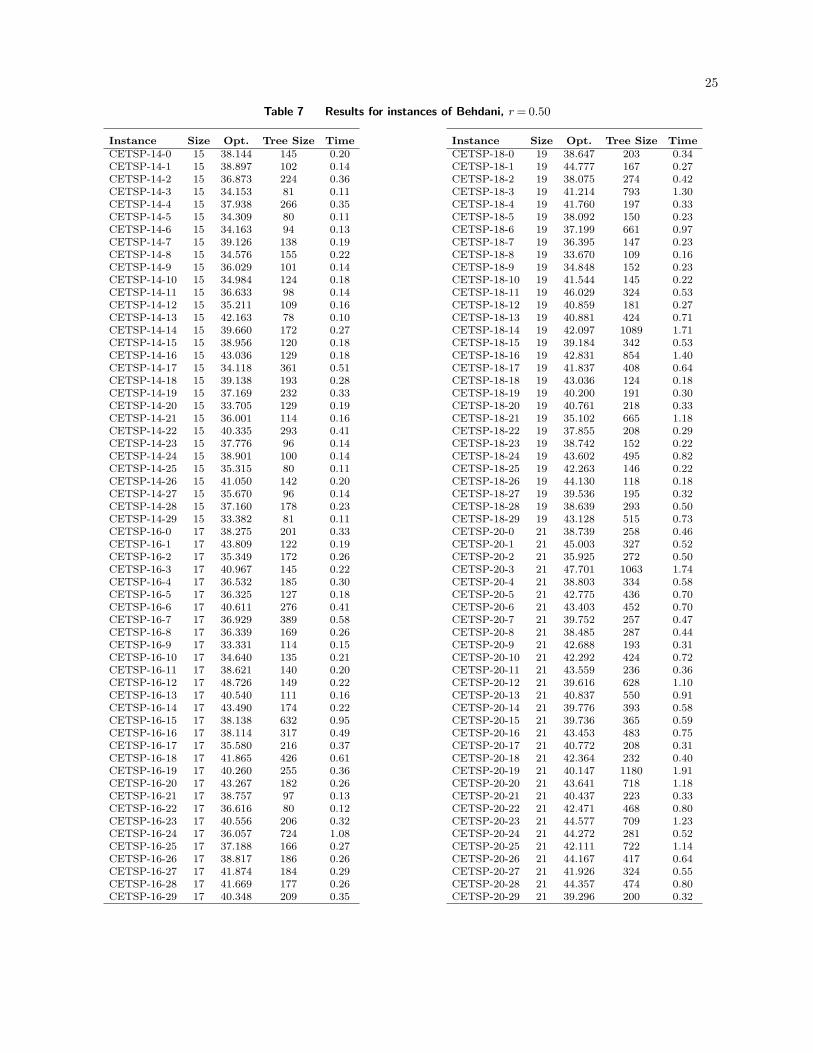
25
Table 7 Results for instances of Behdani, r= 0.50
Instance Size Opt. Tree Size TimeCETSP-14-0 15 38.144 145 0.20
CETSP-14-1 15 38.897 102 0.14
CETSP-14-2 15 36.873 224 0.36
CETSP-14-3 15 34.153 81 0.11
CETSP-14-4 15 37.938 266 0.35
CETSP-14-5 15 34.309 80 0.11
CETSP-14-6 15 34.163 94 0.13
CETSP-14-7 15 39.126 138 0.19
CETSP-14-8 15 34.576 155 0.22
CETSP-14-9 15 36.029 101 0.14
CETSP-14-10 15 34.984 124 0.18
CETSP-14-11 15 36.633 98 0.14
CETSP-14-12 15 35.211 109 0.16
CETSP-14-13 15 42.163 78 0.10
CETSP-14-14 15 39.660 172 0.27
CETSP-14-15 15 38.956 120 0.18
CETSP-14-16 15 43.036 129 0.18
CETSP-14-17 15 34.118 361 0.51
CETSP-14-18 15 39.138 193 0.28
CETSP-14-19 15 37.169 232 0.33
CETSP-14-20 15 33.705 129 0.19
CETSP-14-21 15 36.001 114 0.16
CETSP-14-22 15 40.335 293 0.41
CETSP-14-23 15 37.776 96 0.14
CETSP-14-24 15 38.901 100 0.14
CETSP-14-25 15 35.315 80 0.11
CETSP-14-26 15 41.050 142 0.20
CETSP-14-27 15 35.670 96 0.14
CETSP-14-28 15 37.160 178 0.23
CETSP-14-29 15 33.382 81 0.11
CETSP-16-0 17 38.275 201 0.33
CETSP-16-1 17 43.809 122 0.19
CETSP-16-2 17 35.349 172 0.26
CETSP-16-3 17 40.967 145 0.22
CETSP-16-4 17 36.532 185 0.30
CETSP-16-5 17 36.325 127 0.18
CETSP-16-6 17 40.611 276 0.41
CETSP-16-7 17 36.929 389 0.58
CETSP-16-8 17 36.339 169 0.26
CETSP-16-9 17 33.331 114 0.15
CETSP-16-10 17 34.640 135 0.21
CETSP-16-11 17 38.621 140 0.20
CETSP-16-12 17 48.726 149 0.22
CETSP-16-13 17 40.540 111 0.16
CETSP-16-14 17 43.490 174 0.22
CETSP-16-15 17 38.138 632 0.95
CETSP-16-16 17 38.114 317 0.49
CETSP-16-17 17 35.580 216 0.37
CETSP-16-18 17 41.865 426 0.61
CETSP-16-19 17 40.260 255 0.36
CETSP-16-20 17 43.267 182 0.26
CETSP-16-21 17 38.757 97 0.13
CETSP-16-22 17 36.616 80 0.12
CETSP-16-23 17 40.556 206 0.32
CETSP-16-24 17 36.057 724 1.08
CETSP-16-25 17 37.188 166 0.27
CETSP-16-26 17 38.817 186 0.26
CETSP-16-27 17 41.874 184 0.29
CETSP-16-28 17 41.669 177 0.26
CETSP-16-29 17 40.348 209 0.35
Instance Size Opt. Tree Size TimeCETSP-18-0 19 38.647 203 0.34
CETSP-18-1 19 44.777 167 0.27
CETSP-18-2 19 38.075 274 0.42
CETSP-18-3 19 41.214 793 1.30
CETSP-18-4 19 41.760 197 0.33
CETSP-18-5 19 38.092 150 0.23
CETSP-18-6 19 37.199 661 0.97
CETSP-18-7 19 36.395 147 0.23
CETSP-18-8 19 33.670 109 0.16
CETSP-18-9 19 34.848 152 0.23
CETSP-18-10 19 41.544 145 0.22
CETSP-18-11 19 46.029 324 0.53
CETSP-18-12 19 40.859 181 0.27
CETSP-18-13 19 40.881 424 0.71
CETSP-18-14 19 42.097 1089 1.71
CETSP-18-15 19 39.184 342 0.53
CETSP-18-16 19 42.831 854 1.40
CETSP-18-17 19 41.837 408 0.64
CETSP-18-18 19 43.036 124 0.18
CETSP-18-19 19 40.200 191 0.30
CETSP-18-20 19 40.761 218 0.33
CETSP-18-21 19 35.102 665 1.18
CETSP-18-22 19 37.855 208 0.29
CETSP-18-23 19 38.742 152 0.22
CETSP-18-24 19 43.602 495 0.82
CETSP-18-25 19 42.263 146 0.22
CETSP-18-26 19 44.130 118 0.18
CETSP-18-27 19 39.536 195 0.32
CETSP-18-28 19 38.639 293 0.50
CETSP-18-29 19 43.128 515 0.73
CETSP-20-0 21 38.739 258 0.46
CETSP-20-1 21 45.003 327 0.52
CETSP-20-2 21 35.925 272 0.50
CETSP-20-3 21 47.701 1063 1.74
CETSP-20-4 21 38.803 334 0.58
CETSP-20-5 21 42.775 436 0.70
CETSP-20-6 21 43.403 452 0.70
CETSP-20-7 21 39.752 257 0.47
CETSP-20-8 21 38.485 287 0.44
CETSP-20-9 21 42.688 193 0.31
CETSP-20-10 21 42.292 424 0.72
CETSP-20-11 21 43.559 236 0.36
CETSP-20-12 21 39.616 628 1.10
CETSP-20-13 21 40.837 550 0.91
CETSP-20-14 21 39.776 393 0.58
CETSP-20-15 21 39.736 365 0.59
CETSP-20-16 21 43.453 483 0.75
CETSP-20-17 21 40.772 208 0.31
CETSP-20-18 21 42.364 232 0.40
CETSP-20-19 21 40.147 1180 1.91
CETSP-20-20 21 43.641 718 1.18
CETSP-20-21 21 40.437 223 0.33
CETSP-20-22 21 42.471 468 0.80
CETSP-20-23 21 44.577 709 1.23
CETSP-20-24 21 44.272 281 0.52
CETSP-20-25 21 42.111 722 1.14
CETSP-20-26 21 44.167 417 0.64
CETSP-20-27 21 41.926 324 0.55
CETSP-20-28 21 44.357 474 0.80
CETSP-20-29 21 39.296 200 0.32

26
Table 8 Results for instances of Behdani, r= 1.0
Instance Size Opt. Tree Size TimeCETSP-6-0 7 25.492 21 0.03
CETSP-6-1 7 30.070 7 0.01
CETSP-6-2 7 23.583 7 0.01
CETSP-6-3 7 21.242 7 0.01
CETSP-6-4 7 32.872 11 0.02
CETSP-6-5 7 18.328 33 0.04
CETSP-6-6 7 24.583 11 0.01
CETSP-6-7 7 31.874 7 0.01
CETSP-6-8 7 21.429 7 0.01
CETSP-6-9 7 24.651 3 0.01
CETSP-6-10 7 31.547 3 0.01
CETSP-6-11 7 27.599 7 0.01
CETSP-6-12 7 28.757 21 0.02
CETSP-6-13 7 22.859 11 0.02
CETSP-6-14 7 24.410 7 0.01
CETSP-6-15 7 30.915 21 0.02
CETSP-6-16 7 19.410 3 0.00
CETSP-6-17 7 19.719 3 0.01
CETSP-6-18 7 24.642 21 0.02
CETSP-6-19 7 30.289 1 0.01
CETSP-6-20 7 30.112 21 0.02
CETSP-6-21 7 27.666 33 0.04
CETSP-6-22 7 24.699 11 0.02
CETSP-6-23 7 26.323 21 0.02
CETSP-6-24 7 29.251 11 0.01
CETSP-6-25 7 27.683 3 0.01
CETSP-6-26 7 25.540 21 0.02
CETSP-6-27 7 25.691 32 0.04
CETSP-6-28 7 32.081 11 0.02
CETSP-6-29 7 36.183 21 0.02
CETSP-8-0 9 28.952 16 0.02
CETSP-8-1 9 31.040 40 0.05
CETSP-8-2 9 21.442 11 0.02
CETSP-8-3 9 32.872 11 0.02
CETSP-8-4 9 25.130 22 0.03
CETSP-8-5 9 29.458 7 0.01
CETSP-8-6 9 22.370 21 0.03
CETSP-8-7 9 24.883 16 0.02
CETSP-8-8 9 29.024 16 0.02
CETSP-8-9 9 34.773 21 0.03
CETSP-8-10 9 26.870 7 0.01
CETSP-8-11 9 25.265 47 0.06
CETSP-8-12 9 29.043 21 0.02
CETSP-8-13 9 25.410 33 0.04
CETSP-8-14 9 30.538 69 0.08
CETSP-8-15 9 29.667 33 0.04
CETSP-8-16 9 31.628 16 0.02
CETSP-8-17 9 27.788 11 0.02
CETSP-8-18 9 28.266 33 0.04
CETSP-8-19 9 30.907 21 0.03
CETSP-8-20 9 26.556 21 0.03
CETSP-8-21 9 29.067 33 0.04
CETSP-8-22 9 37.842 12 0.02
CETSP-8-23 9 28.988 27 0.03
CETSP-8-24 9 29.801 7 0.01
CETSP-8-25 9 34.837 46 0.06
CETSP-8-26 9 32.499 33 0.04
CETSP-8-27 9 31.435 26 0.03
CETSP-8-28 9 26.912 16 0.02
CETSP-8-29 9 31.118 7 0.01
Instance Size Opt. Tree Size TimeCETSP-10-0 11 33.676 47 0.06
CETSP-10-1 11 33.975 22 0.03
CETSP-10-2 11 39.391 45 0.06
CETSP-10-3 11 25.712 21 0.03
CETSP-10-4 11 29.385 47 0.06
CETSP-10-5 11 30.549 33 0.04
CETSP-10-6 11 29.905 52 0.06
CETSP-10-7 11 31.081 16 0.02
CETSP-10-8 11 30.131 21 0.03
CETSP-10-9 11 26.385 72 0.10
CETSP-10-10 11 29.958 27 0.04
CETSP-10-11 11 25.754 46 0.06
CETSP-10-12 11 31.008 52 0.06
CETSP-10-13 11 31.673 33 0.04
CETSP-10-14 11 29.243 16 0.02
CETSP-10-15 11 29.146 21 0.02
CETSP-10-16 11 26.944 33 0.04
CETSP-10-17 11 30.583 47 0.06
CETSP-10-18 11 35.006 18 0.03
CETSP-10-19 11 35.341 33 0.04
CETSP-10-20 11 29.807 16 0.03
CETSP-10-21 11 36.794 21 0.03
CETSP-10-22 11 33.030 55 0.07
CETSP-10-23 11 30.539 47 0.06
CETSP-10-24 11 33.796 63 0.08
CETSP-10-25 11 31.857 33 0.04
CETSP-10-26 11 32.308 78 0.11
CETSP-10-27 11 27.130 58 0.08
CETSP-10-28 11 32.835 25 0.03
CETSP-10-29 11 31.368 33 0.04
CETSP-12-0 13 34.781 40 0.04
CETSP-12-1 13 31.290 15 0.02
CETSP-12-2 13 41.043 63 0.08
CETSP-12-3 13 29.392 47 0.06
CETSP-12-4 13 29.861 33 0.04
CETSP-12-5 13 32.559 120 0.18
CETSP-12-6 13 34.125 7 0.01
CETSP-12-7 13 31.965 47 0.06
CETSP-12-8 13 34.148 80 0.11
CETSP-12-9 13 28.670 63 0.08
CETSP-12-10 13 36.543 70 0.09
CETSP-12-11 13 32.700 39 0.05
CETSP-12-12 13 30.844 37 0.05
CETSP-12-13 13 33.012 67 0.09
CETSP-12-14 13 30.262 33 0.04
CETSP-12-15 13 37.461 33 0.04
CETSP-12-16 13 34.406 33 0.04
CETSP-12-17 13 32.065 33 0.04
CETSP-12-18 13 35.911 33 0.04
CETSP-12-19 13 34.633 63 0.08
CETSP-12-20 13 29.612 63 0.08
CETSP-12-21 13 34.539 46 0.06
CETSP-12-22 13 32.308 78 0.11
CETSP-12-23 13 29.230 47 0.06
CETSP-12-24 13 31.748 81 0.11
CETSP-12-25 13 34.127 62 0.08
CETSP-12-26 13 29.896 32 0.04
CETSP-12-27 13 30.937 60 0.08
CETSP-12-28 13 31.753 54 0.07
CETSP-12-29 13 32.269 47 0.06
27
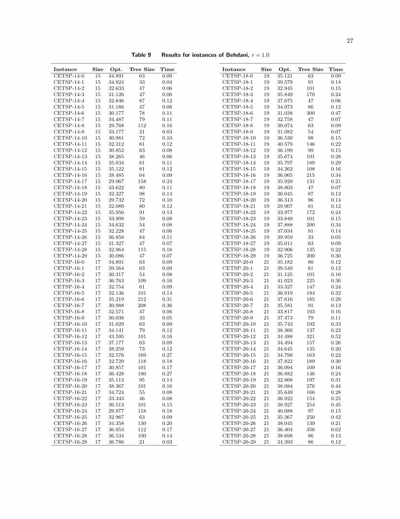
Table 9 Results for instances of Behdani, r= 1.0
Instance Size Opt. Tree Size TimeCETSP-14-0 15 34.891 63 0.09
CETSP-14-1 15 34.924 33 0.04
CETSP-14-2 15 32.633 47 0.06
CETSP-14-3 15 31.126 47 0.06
CETSP-14-4 15 32.846 87 0.12
CETSP-14-5 15 31.186 47 0.06
CETSP-14-6 15 30.177 78 0.11
CETSP-14-7 15 34.487 79 0.11
CETSP-14-8 15 29.768 112 0.16
CETSP-14-9 15 33.177 21 0.03
CETSP-14-10 15 30.981 72 0.10
CETSP-14-11 15 32.312 81 0.12
CETSP-14-12 15 30.852 63 0.08
CETSP-14-13 15 38.265 46 0.06
CETSP-14-14 15 35.034 81 0.11
CETSP-14-15 15 35.122 81 0.12
CETSP-14-16 15 38.485 64 0.09
CETSP-14-17 15 29.067 158 0.24
CETSP-14-18 15 33.622 80 0.11
CETSP-14-19 15 32.327 98 0.14
CETSP-14-20 15 29.732 72 0.10
CETSP-14-21 15 32.089 80 0.12
CETSP-14-22 15 35.956 91 0.13
CETSP-14-23 15 33.998 59 0.08
CETSP-14-24 15 34.632 54 0.08
CETSP-14-25 15 32.228 47 0.06
CETSP-14-26 15 36.858 84 0.11
CETSP-14-27 15 31.327 47 0.07
CETSP-14-28 15 32.964 115 0.16
CETSP-14-29 15 30.086 47 0.07
CETSP-16-0 17 34.891 63 0.09
CETSP-16-1 17 39.564 63 0.09
CETSP-16-2 17 30.317 54 0.08
CETSP-16-3 17 36.763 109 0.16
CETSP-16-4 17 32.754 61 0.09
CETSP-16-5 17 32.136 101 0.14
CETSP-16-6 17 35.219 212 0.31
CETSP-16-7 17 30.988 208 0.36
CETSP-16-8 17 32.571 47 0.06
CETSP-16-9 17 30.038 33 0.05
CETSP-16-10 17 31.029 63 0.09
CETSP-16-11 17 34.141 79 0.12
CETSP-16-12 17 43.595 101 0.16
CETSP-16-13 17 37.177 63 0.09
CETSP-16-14 17 38.259 73 0.12
CETSP-16-15 17 32.576 169 0.27
CETSP-16-16 17 32.729 118 0.18
CETSP-16-17 17 30.857 101 0.17
CETSP-16-18 17 36.428 180 0.27
CETSP-16-19 17 35.113 95 0.14
CETSP-16-20 17 38.367 101 0.16
CETSP-16-21 17 34.724 55 0.08
CETSP-16-22 17 33.343 46 0.08
CETSP-16-23 17 36.513 101 0.15
CETSP-16-24 17 29.977 118 0.18
CETSP-16-25 17 32.967 63 0.09
CETSP-16-26 17 34.358 130 0.20
CETSP-16-27 17 36.953 112 0.17
CETSP-16-28 17 36.534 100 0.14
CETSP-16-29 17 36.786 21 0.03
Instance Size Opt. Tree Size TimeCETSP-18-0 19 35.121 63 0.09
CETSP-18-1 19 39.579 91 0.14
CETSP-18-2 19 32.945 101 0.15
CETSP-18-3 19 35.849 170 0.24
CETSP-18-4 19 37.675 47 0.06
CETSP-18-5 19 34.073 86 0.12
CETSP-18-6 19 31.038 300 0.47
CETSP-18-7 19 32.758 47 0.07
CETSP-18-8 19 30.074 63 0.09
CETSP-18-9 19 31.082 54 0.07
CETSP-18-10 19 36.530 98 0.15
CETSP-18-11 19 40.579 146 0.22
CETSP-18-12 19 36.199 99 0.15
CETSP-18-13 19 35.674 191 0.28
CETSP-18-14 19 35.797 189 0.29
CETSP-18-15 19 34.262 108 0.16
CETSP-18-16 19 36.065 215 0.34
CETSP-18-17 19 35.929 131 0.21
CETSP-18-18 19 38.803 47 0.07
CETSP-18-19 19 36.045 87 0.13
CETSP-18-20 19 36.313 96 0.14
CETSP-18-21 19 29.907 81 0.12
CETSP-18-22 19 33.977 172 0.24
CETSP-18-23 19 33.849 101 0.15
CETSP-18-24 19 37.888 200 0.34
CETSP-18-25 19 37.034 91 0.14
CETSP-18-26 19 39.959 33 0.05
CETSP-18-27 19 35.011 63 0.09
CETSP-18-28 19 32.906 135 0.22
CETSP-18-29 19 36.725 200 0.30
CETSP-20-0 21 35.182 80 0.12
CETSP-20-1 21 39.549 81 0.12
CETSP-20-2 21 31.125 101 0.16
CETSP-20-3 21 41.023 225 0.36
CETSP-20-4 21 33.327 147 0.24
CETSP-20-5 21 36.919 184 0.32
CETSP-20-6 21 37.616 185 0.29
CETSP-20-7 21 35.581 91 0.13
CETSP-20-8 21 33.817 103 0.16
CETSP-20-9 21 37.473 79 0.11
CETSP-20-10 21 35.743 192 0.33
CETSP-20-11 21 38.366 137 0.22
CETSP-20-12 21 34.488 321 0.52
CETSP-20-13 21 34.494 157 0.26
CETSP-20-14 21 34.645 135 0.20
CETSP-20-15 21 34.790 163 0.22
CETSP-20-16 21 37.822 189 0.30
CETSP-20-17 21 36.094 109 0.16
CETSP-20-18 21 36.882 146 0.24
CETSP-20-19 21 32.868 197 0.31
CETSP-20-20 21 38.084 276 0.44
CETSP-20-21 21 35.649 166 0.28
CETSP-20-22 21 36.922 154 0.25
CETSP-20-23 21 38.927 254 0.45
CETSP-20-24 21 40.088 97 0.15
CETSP-20-25 21 35.367 250 0.42
CETSP-20-26 21 38.045 139 0.21
CETSP-20-27 21 36.404 356 0.62
CETSP-20-28 21 38.698 86 0.13
CETSP-20-29 21 34.393 86 0.12

28
References
Andersen, E. D., C. Roos, T. Terlaky. 2003. On implementing a primal-dual interior-point method for conic
quadratic optimization. Math. Programming 95(2) 249–277.
Applegate, D. L., R. E. Bixby, V. Chvatal, W. J. Cook. 2011. The Traveling Salesman Problem: A Compu-
tational Study (Princeton Series in Applied Mathematics). Princeton University Press.
Arkin, E., R. Hassin. 1994. Approximation Algorithms For The Geometric Covering Salesman Problem.
Discrete Applied Mathematics 55(3) 197–218.
Behdani, B., J. C. Smith. 2013. An Integer-Programming-Based Approach to the Close-Enough Traveling
Salesman Problem. INFORMS J. Comput. Forthcoming.
Bodin, Peter. 2009. BUBBLEPLOT3: A simple 3D bubbleplot. http://www.mathworks.com/
matlabcentral/fileexchange/8231-bubbleplot3.
Boyd, S., L. Vandenberghe. 2004. Convex Optimization. Cambridge University Press.
Dong, J., N. Yang, M. Chen. 2007. Heuristic Approaches for a TSP Variant: The Automatic Meter Reading
Shortest Tour Problem. Extending the Horizons: Advances in Computing, Optimization, and Decision
Technologies, vol. 37. Springer US, 145–163.
Farid, A., D. Goldfarb. 2003. Second-order cone programming. Math. Programming 95 3–51.
Gendreau, M., G. Laporte, F. Semet. 1997. The Covering Tour Problem. Oper. Res. 45(4) 568–576.
Gulczynski, D. J., J. W. Heath, C. C. Price. 2006. The Close Enough Traveling Salesman Problem: A
Discussion of Several Heuristics. Perspectives in Operations Research, vol. 36. Springer US, 271–283.
Ha, M. H., N. Bostel, A. Langevin, L. Rousseau. 2013. Solving the close-enough arc routing problem.
Networks Forthcoming.
Lobo, M.S., L. Vandenberghe, S. Boyd, H. Lebret. 1998. Applications of second-order cone programming.
Linear Algebra Appl. 284(1-3) 193–228.
Mennell, W. 2009. Heuristics for solving three routing problems: Close-Enough Traveling Salesman Prob-
lem, Close-Enough Vehicle Routing Problem, Sequence-Dependent Team Orienteering Problem. Ph.D.
thesis, University of Maryland, College Park.
Mennell, W., B. Golden, E. Wasil. 2011. A Steiner-Zone Heuristic for Solving the Close-Enough Traveling
Salesman Problem . 12th INFORMS Computing Society Conference: Operations Research, Computing,
and Homeland Defense. Monterey, California.
Shuttleworth, R., B. Golden, S. Smith, E. Wasil. 2008. Advances in Meter Reading: Heuristic Solution of
the Close Enough Traveling Salesman Problem over a Street Network. The Vehicle Routing Problem:
Latest Advances and New Challenges, vol. 43. 487–501.
Silberholz, J., B. Golden. 2007. The Generalized Traveling Salesman Problem: A New Genetic Algorithm
Approach. Extending the Horizons: Advances in Computing, Optimization, and Decision Technologies,
vol. 37. Springer US, 165–181.
29
Yuan, B., M. Orlowska, S. Sadiq. 2007. On the optimal robot routing problem in wireless sensor networks.
IEEE Transactions on Knowledge and Data Engineering 19(9) 1252–1261.