DISCRETE APPLIED MATHEMATICS

ELSEVIER Discrete Applied Mathematics 94 (1999) 77 99

A branch and bound algorithm for a single-machine scheduling problem with positive and negative time-lags

Reccivcd 30 October 1996: revised 2 July 1997; accepted X I\,lay I99X

Abstract

Positive and negative time-lags are general timing restrictions between the starting time>

of jobs which have been introduced by Roy in connection with the Metra Potential Method.

They allow the consideration of positive and negative time-lags between the starting times ol

jobs. It is shown that complex scheduling problems like general shop problems, problems with

multi-processor tasks, problems with multi-purpose machines. and problems with changeok er

times can be reduced to single-machine problems with positive and negative time-lags between

jobs. Furthermore. a branch and bound algorithm is developed for solving such single-machine

scheduling problems. The reductions can be used to construct test problems for this algorithm

Computational results for randomly generated single-machine problems and for shop scheduling

problems (without time-lags) are reported. 0 1999 Else\ier Science B.V. All rights reserved.

,G’SC’: 90B35

K~y~~wtl.c: Time-lags; Branch and bound; Scheduling; Shop problems: Multi-purpose machines:

Multi-processor tasks

1. Introduction

In connection with project planning, Roy [21] developed the Metra Potential Method

(MPM). In his model he uses two types of relations between jobs or activities. The tirst

type expresses that between the starting points of two jobs there must be a minimal

time-lag. The second stipulates that there must be a maximal time-lag. The model may

be formulated as follows. Let J = { 1, , II} be a set of n jobs to be scheduled without

preemption. Let S, be the starting time of job i. Then the completion time C, of job i

Supported by the Deutsche Forschungsgemeillschaft. Project ‘Komplexc Maschinen-SchedulinFproblclne’ * Corresponding author. Tel.: +49 541 969 2538: fax: +49 541 969 2770:

E-nzrril trtlr/w\r: Pcter.Brucker~mathematik.uni-osnabrueck.de (P. Bruckcr)

0166.218X/99/$ see front matter 0 1999 Elaevier Science H.V. All rlyhts rcsened

I’ll: sol6~-2lxx(Y9)oool5-3

78 P. Brucker et ~11. I Di.wrrre Applied Mathetnutics 94 (1999) 77-99

is given by Ci = Si + pi where pi denotes the processing time of i. Furthermore, a set

R of relations of the form

S;+I,,<S’i (i,j)~RcJxJ (‘I

exists where 1, is a given arbitrary integer number. A relation of type (1) is called a

start-start relution between job i and j. If lija 0, then (1) means that job j cannot

be started earlier than 1l.j time units after the starting time of job i (minimal time-lag).

On the other hand, if 1, < 0, then job j cannot be started earlier than )l,] time units

before the starting time of job i (maximal time-lag).

The relations (1) are very general timing relations between jobs. For example, (1)

with iii = p; means that job j cannot start before job i finishes. More generally, if

there should be a minimal time distance of d;, units between the completion of job

i and the start of job j, then we write Si + pi + d,, ,< S,. If S, + pi + dii d Sj and

Sj - u,i - p; < 5’; hold, where 0 d d, d Uij, then the time between the finishing time

of job i and the starting time of job j must be at least dij but no more than Ulj. This

includes the special case 0 d d, = uii where job j must start exactly dii time units

after the completion time of job i. Also release times q and deadlines di of jobs i

can be modeled by the relation (1) (see [ 11). Positive and negative time-lags are also

used to describe timing restrictions for industrial production processes (e.g. in chemical

production or the steel industry).

Balas et al. [25] considered the single-machine problem with heads and tails

1 l%qi/Glax with positive time-lags only. They propose an efficient adaption of Car-

lier’s algorithm for the problem without time-lags (see [9]) and show that the cor-

responding preemptive problem is .I“.9-hard. Scheduling problems with positive and

negative time-lags have mainly been discussed in connection with project scheduling

[ 1,3,11,12,20,24]. They are usually very hard to solve. The work of Wikum et al.

[23] may explain this observation. They investigated the complexity of single-machine

problems with minimal and/or maximal distances between jobs. Their main results

show that scheduling problems of this type with a very simple structure are already

., l’p-hard.

In this paper we investigate single-machine and parallel-machine scheduling problems

with constraints of the form (1). For the single-machine problem an n-tuple (Si) is

called a feasible schedule if

l for all i # j the intervals [Si, S, + pL[ and [S,, S, + p,[ are disjoint and

l the conditions (1) are satisfied.

The basic problem we consider is

P: We are given jobs 1,. . . , n with processing times pi (i = 1,. . . , n) to be processed

on a single machine and relations of type (1). Find a feasible schedule (Si) which

minimizes the makespan C,,, = max:=,{S! + pi} if such a schedule exists.

As mentioned above, it is possible to model release times and deadlines by con-

straints of type (1). This implies that, in general, not only the problem of finding an

optimal solution but also the problem of just finding a feasible solution is :,l’g-hard.

Thus, no simple heuristic to derive feasible solutions will be available.

Firstly, we will show that complicated parallel-machine problems and shop schedul-

ing problems can be polynomially reduced to problems P. Among these problems

are general shop problems, problems with multi-processor tasks. problems with multi-

purpose machines, problems with sequence-dependent changeover times. and combi-

nations of these problems which have been considered in connection with Rexible

manufacturing systems. Since problem P is I ‘Y-hard the existence of such reductions

is obvious. However, the described reductions are quite direct and usually do not in-

crease the size of the problems considerably. These quite surprising results are mainI>

of theoretical interest.

In the second part of the paper we will develop a branch and bound proccdurc for

problem P. Unfortunately, no benchmark problems for P exist and randomly generated

test data tend to be easy. Therefore we use open-shop and job-shop problems (with

classical precedence relations only) which are transformed into single-machine problem\

with positive and negative time-lags as test problems.

The organization of the rest of this paper is as follows. In Section 2 we will dc-

scribe the reductions of complex scheduling problems to the single-machine problem

with constraints of the form (1). In Section 3 we will sketch the main parts of

the developed branch and bound method. Afterwards, in Section 4. we will report

on computational experiments with the branch and bound method. The paper ends

with some concluding remarks. Within the next sections we assume that all data are

integers.

2. Reduction of scheduling problems with start-start relations

In this section we will describe how general shop problems, problems with multi-

processor tasks, problems with multi-purpose machines, and single-machine problems

with sequence-dependent changeover times may be reduced to a single-machine schedul-

ing problem with relations of type (1). The reductions consist of two steps. In the tirst

step the complicated scheduling problem will be reduced to a scheduling problem with

parallel dedicated machines. In the second step the scheduling problem with parallel

dedicated machines will be reduced to the single-machine problem.

The problem n,ith parullel &dicattd tmd~inrs can be described as follows. We are

given m parallel machines h-l,, . , M,,, and jobs I,. . , t7 with processing times !I, (i

I.. . ,t7) where job i can only be processed on a specific machine M,,, (LL~ t { I,. .,w) ).

Furthermore, there are relations (I ) given between the jobs. Find a feasible schedule

which minimizes the makespan. A schedule is feasible it’jobs to be processed on the

same machine do not overlap and the relations (I ) are satisfied.

To reduce this problem to a single-machine problem. let UB be an upper bound for

the minimal makespan of the parallel dedicated machine problem under the assumption

80 P. Brucker et al. I Discrete Applied Mathematics 94 (1999) 77-99

that a feasible schedule exists. We may choose, for example,

The idea of the reduction is for each machine A4j to translate the schedule on this

machine into the interval [(j - l)UB, jUB]. More specifically, if (Si) is a schedule

for the parallel dedicated machine problem, then we transform this schedule into a

schedule (S:) for the single-machine problem with

S,!=Si+(/L-I)UB fori=l,...,n.

By this transformation the relation S; + lij < Si translates to

(2)

or equivalently

S,! + Iii + (pj - p;)UB < 5’;.

To ensure that a job i to be processed on MPA is really scheduled in [(,LL~ - l)UB,piUB] by (S:) we introduce a dummy job 0 with pa=0 and add the following two restrictions:

S’h + (pi - l)UB < St’, (3)

S,( - PiUB d SA. (4)

It is not difficult to see that (S,) is a feasible schedule for the parallel dedicated machine

problem if and only if Si is a feasible schedule for the single-machine problem.

To reduce the C ,,X-problem for parallel dedicated machines to a single-machine

problem we first add a dummy job n + 1 with processing time pn+r = 0 to be processed

on machine Mm. For each job i = 1,. . , IZ we add the relation

Si + pi d Srz+l. (5)

Due to the restrictions (5) the minimal makespan Cmax of the original problem is equal

to the minimal makespan of the augmented problem which is identical to the minimal

finishing time of the dummy job n + 1. Moreover, the minimal finishing time CL,, of

the single-machine problem we get by transforming the augmented problem is given

by

CL,,, = C,,,,, + (m - 1)UB.

Finally, we would to note that for the C,,, -objective our reduction transforms a parallel

dedicated machine problem with n jobs and k start-start relations into a single-machine

problem with n + 2 jobs and k + 3n start-start relations.

2.2. Generul shop problems

The general shop problem with start-start relations can be formulated as follows.

We are given n jobs 1,. . , n to be processed on m machines Ml,. . . ,A4,. Job i consists

of fl, operations O,I , . . . , Oi,, with processing times p,, ( j = 1,. . , n,). Associated with

each operation 0,, there is a dedicated machine MI,,; on which 0,, must be processed

without preemption. No two operations of the same job and no two operations to be

processed on the same machine can overlap. There are start-start relations between the

operations. General shop problems have been introduced by Kleinau [17].

We want to reduce the general shop problem with start-start relations and the C‘,,,,,,

objective to parallel dedicated machine problems with 17 t 177 machines. Machines

hl,, . , M,,, correspond with the machines of the general shop problem and machines

MI,, ,~ I > . ~~,I, , ,i are associated with the jobs I,. .I?. For each operation 0,, WC create

two jobs:

J,: with pj, = pli and ,D:, = /lli

and

JIS with pf, = pii and ,~f, = IV + i.

Furthermore, we force each pair of jobs J,) and J,; to start at the same time by intro-

ducing two start-start restrictions. Finally, we define start-start relations between jobs of

the form J1) and Jj, if and only if start-start relations exist between the corresponding

operations 0,, and Ok/.

The jobs Jii guarantee that operations to be processed on the same machine do

not overlap. The jobs Jl; guarantee that operations belonging to the same job do not

overlap.

Clearly, the general shop problem has a feasible solution if and only if the corre-

sponding problem with parallel dedicated machines has a feasible solution and in that

case the optimal C,,,, -values of both problems are equal.

If the general shop problem has 1 operations and k start-start relations, then it reduces

to a parallel dedicated machine problem with 21 jobs and k + 21 relations or to a

single-machine problem with 21 + 2 jobs and li + 81 relations.

2.3. Prohlenl,v Ir’itll ndti-procrssor triskh

A ~nulti-l”o”““sor tusk scheduling prohh is given as follows. There are n tasks

1.. ,n with processing times ~1,. . , pn and m machines MI,. ,M,,,. Associated with

each task i there is a set of machines ..1/, := {M,, , . , M,,, }. Task i needs all machines

in set -0’; during a processing period of length p,. Thus, jbbs i and .j with I /Ii I?. 4, # ti

cannot be processed simultaneously. There are start-start relations between the tasks.

Again, the C,,,,,-p roblem is to be solved. Problems of this type have been studied

recently e.g. by Blaiewicz et al. [2] and Hoogeveen et al. [IS].

To reduce this problem to a problem with m parallel dedicated machines MI.. , !A!,,,.

for each task i = I,. . . , n we introduce ni jobs J,‘. ,J,“’ with

Pi = PI and ~1: = i,.

j = I.. . II,. By 2(n, - I ) start-start relations all jobs J,‘, .J,“’ are forced to start at

the same time.

82 P. Brucker et al. IDiscrete Applied Muthemotics 94 (1999) 77-99

Finally, we define a start-start relation between jobs J,’ and Jj if and only if there

is a corresponding start-start relation between i and j.

Clearly, both problems are equivalent.

If the multi-processor task problem has u tasks and k relations, and if nl, . . . , n,

are the cardinalities of the machine sets ~&‘i (i = 1,. . . , n) then the parallel dedicated

machine problem has C:=, ni jobs and 2 Cr=, (ni - 1) + k relations. The corresponding

single-machine problem has c:=, IZ~ + 2 jobs and 5 EYE, ni + k - 2n relations.

2.4. Multi-purpose machines

A multi-purpose machine problem is defined as follows. Given are n jobs 1,. . . , n

with processing times ~1,. . , pn and m machines MP,, . . . , MP,,,. Associated with each

job i there is a set &‘i = {MPi,, . . . ,MPi,>, } &{MPl, . . . ,MP,} of machines. We have

to assign job i to exactly one single-machine from &‘i. Jobs assigned to the same

machine cannot overlap. There are start-start relations between the jobs. The goal is to

minimize the makespan. Multi-purpose machine problems of the above type have been

studied by Brucker and Schlie [8] and Jurisch [16].

To reduce the multi-purpose machine problem to a problem with parallel dedicated

machines we create n + k + 1 such machines where k is the number of start-start

relations. The reduction is undertaken in such a way that scheduling a job in time

period [ j(2UB + I) - UB, j(2UB + l)] where 1= max{ iljil} is equivalent to scheduling

the job on machine MPj.

The first n machines M, (i = 1,. . ,n) correspond with the jobs i. M, takes care of

the assignment of job i to some machine in ./Z’i. Associated with M, there are n; + 1

dummy jobs D~,...,D~“‘. The idea of the dummy jobs is to block on machine M, all

time periods except time periods of the form [j(2U3 + I) - UB, j(2UB + l)] which

correspond with the multi-purpose machines MPj E Ai. As before, UB is an upper

bound for the C,,, -value of the original problem. More specifically, dummy job D/

has the processing time [(ij ~ ii_l)(2UB + 1) - UB] and is forced by two start-start

relations to start at time ii-1 (2UB+/) forj= l,...,ni+ 1, io:=O, in,+* =m+ 1. Job

i is dedicated to machine Mi and must be scheduled within [O,m (2UB + /)I. Thus,

scheduling job i is equivalent to scheduling i on some machine in ./Yi.

Example. Consider a job i with -&‘i = {MP~,MP~,MPA}. The corresponding dummy

jobs D~,D?,D~,Df are shown in Fig. 1.

To avoid two jobs to be processed on the same machine MPj from overlapping we

introduce a machine M,, 1 and replace each job i by two jobs J,’ and Jf to be processed

Fig. I

x3

Fig. 2

Fig. 3.

for pi time units simultaneously on M, and A4,1+l, respectively. Thus, the schedule on

machine MP, is transformed to the schedule in the ,j-th interval on machine .U,, , ,

Finally. we must explain how start-start relations

are respected in the parallel dedicated machine problem.

Since we do not know in advance to which machine, i.e. to which time slot

[,j(2UB + 1) - UB,j(2UB + l)] a job is assigned, we cannot transform the relation

(6) directly into a start-start relation for the parallel dedicated machine problem.

Before describing how to solve this problem we will describe a technique to simulate

a start-start relation (6) by two dummy jobs on an additional dummy machine.

Due to the relation (6) we have to block the time interval [O,s, + I,,] for job j if

.job i starts at time s,. This can be realized by a job A,,, with processing time UB and

a job Aif2 with processing time p,, both to be processed on the dummy machine. Job

A /,I is forced to start exactly UB - I,, time units before job i and job A,il is forced

to start at the same time as job ,j. We claim that the dummy jobs and the dummy

machine guarantee that the relation (6) is satisfied.

If I,, 20, we have a situation as shown in Fig. 2.

Thus, A,,? cannot start earlier than I,, time units after 3, which means that (h) is

satisfied.

If I,, < 0, we have a situation as shown in Fig. 3.

Again, A,,? cannot start earlier than at time ii + I,, which means that (6) is satisfied.

To take care of the start-start relations of the multi-purpose machine problem WC

will use the introduced concept of dummy jobs and machines. However, instead of two

dummy jobs A,,, and Ai,2 we will introduce I~Z ‘copies’ AI,,. ,. 4”’ and Al,,.. ., ,,, )I”’ ,,:

of these jobs scheduled with distance 2C’B + 1 between the copies. More specifically,

for each relation (6) we add a machine M,, and jobs A:,,.. , AyiI. for 11 _ I, 2 to be

processed on ltl,,. By start-start relations

. Al,, is forced to start exactly UB ~ I,, time units bet’ore ,/,I.

l ,4,‘,, and J,’ are forced to start at the same time.

84 P. Brucker et cd I Discrete Applied Murhwnatics 94 (1999) 77-99

Fig. 4.

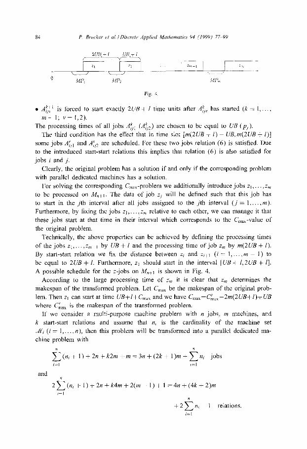
l A!+’ is forced to start exactly 2UB + 1 time units after A!,,, has started (k = 1,. . , !I ” m - 1; v= 1,2).

The processing times of all jobs AtI (A&) are chosen to be equal to c/B (p,).

The third condition has the effect that in time slot [m(2UB + I) - UB,m(2UB + l)]

some jobs Ari, and A$ are scheduled. For these two jobs relation (6) is satisfied. Due

to the introduced start-start relations this implies that relation (6) is also satisfied for

jobs i and j.

Clearly, the original problem has a solution if and only if the corresponding problem

with parallel dedicated machines has a solution.

For solving the corresponding C,,,-p roblem we additionally introduce jobs zi , . . . ,z,

to be processed on A&+,. The data of job z, will be defined such that this job has

to start in the jth interval after all jobs assigned to the jth interval (j = 1,. . , m).

Furthermore, by fixing the jobs ~1,. . . , z,, relative to each other, we can manage it that

these jobs start at that time in their interval which corresponds to the C&,-value of

the original problem.

Technically, the above properties can be achieved by defining the processing times

of the jobs zI,. ,z,,_, by UB + 1 and the processing time of job z, by m(2UB + 1).

By start-start relation we fix the distance between z; and zi+l (i = 1,. . . , m - 1) to

be equal to 2UB + 1. Furthermore, zl should start in the interval [UB + 1,2UB + I].

A possible schedule for the z-jobs on IV,,+, is shown in Fig. 4.

According to the large processing time of z, it is clear that z, determines the

makespan of the transformed problem. Let C,,,,, be the makespan of the original prob-

lem. Then ZI can start at time UB+l+C,,,,, and we have C,,,,,=C~,,,-2m(2UB+l)+UB

where C&,, is the makespan of the transformed problem.

If we consider a multi-purpose machine problem with n jobs, m machines, and

k start-start relations and assume that n, is the cardinality of the machine set

U+Yi (i= l,..., n), then this problem will be transformed into a parallel dedicated ma-

chine problem with

~(ni+l)+2rr+k2m+m==3n+(2k+I)m+~n~ jobs i=l 1-l

and

2e(ni+ 1)+2n+k4m+2(m- 1)+1=4n+(4k+2)m i=l

n

+2zniP1 relations. i=l

The corresponding single-machine problem has

2 + 3/? + (2/i + 1 )UZ + C4 jobs i-l

and

1 3n + ( 1 Ok + 5)~ - 1 + 5 1 II, relations. i I

Consider II jobs i = 1,. , II with processing times /II,. . pIi to be processed on

a single machine. The set of all jobs is partitioned into r groups GI,. , G,.. By

~1~ E {G,, . . G,.} we denote the group to which job i belongs. If a job ,i from group

Gi is processed immediately after a job i from group G,, there is a setup time .X/A. i.e.

job ,j starts at the earliest S/k time units after the finishing time of job i. We set s/l = 0

for all I = I,. , I’ and assume that the s/i-values satisfy the triangle inequality, i.e.

,s/i; -t .sk/, >s//~ for all I, k, h t { 1, . 1.).

The problem of finding an optimal schedule for this problem under various objective

functions has been studied by Monma and Potts [ 191.

We assume that start-start relations between the jobs are additionally given and that

we are interested in solving the C,,;,,-problem. A reduction of this problem to a problem

with parallel dedicated machines is undertaken as follows.

All jobs i = I,. . n must be processed on a first machine MI. Furthermore. for each

pair i.,j of jobs belonging to different groups (i.e. 61; j; (1,) we introduce a machine

M,,. On this machine two jobs J;, and ,I(: with processing times ~1, +s~,~!,, and /l, -~ v,,,,,

must be processed. By start-start relations jobs .I,‘, (Jr: ) and i (,j) are forced to start

at the same time. Furthermore, we have the start-start relations defined between job5

I,....n.

Jobs J;, and .I,: take care of the changeover times between jobs i and ,i. Notice that

there is also a “changeover time” on machine IV,, if j is processed after i but not

immediately after i. Due to the triangle inequality there are no problems with these

types of changeover times.

To solve the corresponding C,,,,-p roblem we add a dummy job n+ 1 with processing

time p,!, I = s := max,.,s,, which must be a successor of each other job and is to be

processed on Ml. The makespan C,&, of the parallel dedicated machine problem is

given by the makespan on MI and we have

where C,,,,, is the makespan of the original problem. If the dummy job II + I has a

processing time smaller than S, it could happen that one of the jobs introduced to model

the setup times determines the makespan of the parallel dedicated machine problem.

P. Bucker ct ul. I Discrete Applied Mathrmatics 94 11999) 77-99

For a problem with n jobs, group sizes nl,. . ,n,, and k start relations we get a

parallel dedicated machine problem with

c nlnk f 1 machines,

lik

n+l+n*-En; jobs i=l

and

k+n+2 .?-kr$ ! i

start-start relations. i=I

3. A branch and bound algorithm

In this section we will present a branch and bound method for a single machine

problem with start-start relations. The techniques used are similar to those in [5,7].

However, a significant difference between the developed branch and bound method

and most other branch and bound methods is the upper bounding. Since the problem

of finding a feasible solution is ,VY-hard, we are not able in each search tree node

to calculate a feasible solution heuristically. Feasible solutions are only found in the

leaves of the search tree. This will lead to a different approach to organize the branch

and bound method.

This section is organized as follows: In Section 3.1 we will introduce a graph model

which is used to represent instances of the problem. Afterwards, in Section 3.2 adapted

concepts of immediate selection will be presented. Finally, in Section 3.3 two different

branch and bound procedures are given.

3.1. Disjunctive graphs

We have introduced a single-machine problem with start-start relations Si + 11, < Si

between jobs i,j with i # j. If I,> 0, this relation means that job j cannot be started

earlier than IV time units after the starting time of job i. If 1, < 0, then job i cannot

start later than -1, time units after the starting time of job j.

Additionally, in this problem we will introduce two dummy jobs 0 and n + 1 with

processing times zero. Job 0 is a starting job which must be “processed” before all

other jobs i (i.e. loi = 0) and job n + 1 is a final job which must be “processed’ after

all other jobs i (i.e. lr,n+l = pi ) Furthermore, we may assume that for each job-pair

(i,j); i,j=O,. ., n + 1; i # j a relation S, + iii < Sj is defined (if this is not the case,

we introduce a redundant relation with fv = -,xX)).

Next we associate with the start-start relations R a network N(R) which is defined

as follows:

l the vertex set Y = (0, 1, . . , n, n + l> consists of all jobs 1,. . . , n and the two dummy

jobs 0 and n + 1

l for each pair (i,,j) of jobs i, j = 0,. . . . n+ 1 with i # j there is an arc (i.,j) of length

I,,. Under the assumption that there are sufficient machines (e.g. n machines) available

which can process the jobs in parallel the problem has a feasible solution if and

only if the corresponding network contains no positive cycle. In this case a schedule

minimizing the makespan can be constructed by

l calculating the length I(i) of the longest path from the starting job 0 to job i for all

jobs i= I....,n,

l starting job i at time I(i) for i = 1,. . . , n.

Furthermore, the length of a longest path from the starting job 0 to the final job t? + I

corresponds to the minimal makespan.

If we have only one machine on which all jobs must be processed, we have to

avoid jobs overlapping by adding relations of the form S, + p, < S,. Here adding

means replacing the relation S; + I,, < S, by

S, + max{ p,, I,/} < S,.

The branch and bound algorithm which will be developed adds step by step relations

of the form S, + pI < Sj which do not create positive cycles in the actual network. In

connection with this it is useful to introduce the concept of disjunctive graphs.

We call the complete undirected graph G==( V, E) with vertex set V={O, 1.. . tt. tt - I }

and edges {i,,j} (i,,j E V, i # j) a &sjtmcriz:e y~upl~. The edges {i, j} of G are called

di~juncfiw puirs. The basic scheduling decision is to ,fis a disjunctive pair by adding

either the relation Si + p; < S, or the relation S, + ~7, < S,. A set L of relations which

correspond to fixed disjunctions is called a selection. A selection L is called ~orll$r~tc

if

l each disjunctive arc is fixed by L,

l the network resulting by adding L to the given start-start relations has no positive

cycles.

The branch and bound method branches by fixing disjunctive pairs in either direc-

tion. Another method of fixing disjunctive pairs is immediate selection. By immediate

selection disjunctive pairs will be fixed on the basis of the existing start-start relations.

3.2. Itntnerliate .selection

A first simple way to tighten the start-start relations is to replace I,, by the length

of a longest path from i to j in the network. Using these values a simple condition

under which a disjunctive pair can be fixed is given by

Lemma 1. The rkjunctive puir {i, j} cm he ,fised hy uddiny S, + pi < S, if

(7)

88 P. Brucker et al. I Discrete Applial Muthenwtics 94 (1999) 77-99

The proof of this lemma is straightforward and can be found in a former version of

this paper [4] or in [ 1 I].

Another method for tightening the start-start relations uses relative time windows

between the jobs (see [I]). Relative to job k, job i has to be processed in the time

window [& + rlk, & + df], where i-k = lki and df = pi - lik. Thus, if we fix some arbi-

trary job k (e.g. define &. = 0), all jobs have time windows in which they have to be

processed. Based on these time windows [r/,df] for the jobs, we will introduce two

techniques (i) and (ii) to tighten the given start-start relations. The first technique is

similar to a method of Carlier and Pinson [lo] introduced for the job-shop problem.

Both techniques use a method of Brucker et al. [6] which calculates for a given time

interval I = [a,h] and a given subset A4 of jobs a lower bound Ba for the total

time in which jobs from A4 must be processed in I if they respect their time windows.

The bound can be calculated in 0( 1Mllog in/r]) time.

(i) Let I = [a, 61 be an arbitrary time interval and let j E { 1,. . . , n} \ hf. Assume

that a + Ba + p, > h. Then job ,j cannot be scheduled completely in I and either has

to start before h - Bf, - p,i or after a f B$,,.

We now consider two cases. Firstly, assume that rf > b ~ Bf, - pj. In this case job

j cannot start before b ~ BL - pi and therefore has to start after a + Ba. Thus, we

can replace yr by $ := max{rr, a + Bk} and therefore lkj by i&i := max{ lkj, a + BL}.

Next, we assume that d; < a+Ba+p,i. Now job j cannot start after a+Bf, and there-

fore has to start before b - Bh - p,. Thus, we can replace di by d: := min{di, b - Bh}

and therefore l/k by ijk := max{ l,k, -(b ~ Ba - pi)}.

(ii) Let A4 be an arbitrary subset of jobs, let i, j (i # j) be two jobs not in M, and

let I = [r,!,d$]. Assume that we try to fix the disjunctive pair {a j} by processing job

i before job ,j. Then both jobs must be processed within the time window [r/‘,df]. If

now Bf, + pi + pj > d.f - r/ then it is not possible to process i before j and we can

fix the opposite disjunction. Thus, we can replace lji by iji := max{pi, I,;}.

In the branch and bound procedure these techniques were tested with the following

sets M and intervals I:

(a) technique (i) with 1 = [~/,df], M = { 1,. . . ,n} \ {j}, where j is a job with

[rj,d;] nZ # 0.

(b) technique (i) with I = [r/,d:], i # 1, M = { 1,. . , a} \ {,j}, where j is a job with

[$, d,k] n I # 0. (c) technique (ii) with A4 = { 1,. . . ,n} \ {i,,j}.

Checking (a) and (b) for all possible intervals I can be realized in an overall com-

plexity of 0(n2). The same complexity is needed to check (c) for all possible intervals

I (see [6]).

3.3. Brunch and bound procedures

In this section some experience with branch and bound procedures for solving prob-

lem P will be reported. We first developed a basic algorithm which we call the

a-procedure. It turned out that the x-procedure was not very efficient. For these rca-

sons we developed a P-procedure which is a more sophisticated algorithm using the

%-procedure as a subroutine.

3.3.1. T/w r-pwmhre

The z-procedure is a branch and bound algorithm which branches on disjunctive

pairs {i,,i}. This means that if neither I,, 2 p, nor I, 2 p, then the current problem.

given by an network N, is split into two subproblems given by networks ;VI and 9’2.

N, is derived from N by adding the relation S, + p, < S,, N? is derived by adding

s, + /I, < s, We describe the procedure recursively. Let the current problem be given by an

network N and assume that we have some upper bound UB for the optimal C,nax-~al~e.

(The calculation of an initial upper bound will be presented later on in this subsection.

With the lapse of time, UB is the makespan of the best feasible solution found so far. )

Because we wish to improve the upper bound we define the length of the (II + I. 0 )

by I,, , I.,, = ~-- (L/B ~ 1) which corresponds to the start-start relation

‘,>+, <so+c/B- 1. 7

Next we apply the Procedure Immediate Selection to N. If this yields a complete

selection S, we have a new feasible solution and update the UB-value. Otherwise.

we apply some infeasibility tests. If one of these tests proves infeasibility. we can

leave the current search tree node. Otherwise, the problem may be feasible or not and

we have to select a disjunctive pair for branching.

For the choice of the disjunctive pair we use the time windows which restrict the

starting times of the jobs relative to each other. We analyze for each pair how far

the starting time of the corresponding jobs are restricted by such time windows. More

precisely, for each disjunctive pair (i, li) of jobs we calculate the number I’,” of possible

integer starting points S, for job i within the time interval [~,“.u’f;] and nolmalizc thi5

number by the sum of the processing times of jobs i and li.

Since [~./.cIf] repr esents the time interval in which job i has to be processed if job

X- is processed in [0, ok] (assuming Sk = O), and since (i,k) is a disjunctive pair. we

have I’, < - [J, or df 3 pk + p,. Thus, we have

.r.; = (~-Pi - li *’ + 1) + (df - 17; ~ pi< + I) -l,L -- IA, ~ /?I ~ ph- -t 2

pi + Pk /‘I + Ph

(see Fig. 5).

We choose a disjunctive pair where the jobs are not too restricted (for restricted Jobs

the corresponding disjunctive pair will probably be fixed by immediate selections in

one of the following search tree nodes) and are also not too unrestricted (a restriction

of such unrestricted jobs by fixing a disjunction may prevent us from finding a feasible

solution). We have tried to realize these principles as follows: We calculate for each

job i the median of all ,ft-values, select a job i with the smallest median, choose i

as the job with the smallest .f,‘-value. and select the disjunction (i, i) as the pair for

90 P. Brucker et al. I Discrete Applied Mathematics 94 11999) 77-99

Fig. 5.

branching. A detailed description of this process can be found in [14]. After choosing a

disjunctive pair the two corresponding subproblems Ni and N2 are created and treated

recursively.

We still have to explain how to implement the infeasibility tests. One part of this

test is already incorporated into the immediate selection procedures. If the bound BL

calculated by one of the techniques (i) or (ii) is larger than the length of the interval

I, no feasible solution exists.

Two further tests have been used jointly.

(1) We test whether the network contains a positive cycle.

(2) For each job k we do the following: We calculate the time window [Y!, ~$1 of job

i with respect to job k for each job i. Then we solve a corresponding single-machine

problem 1 / Yj; pmtn 1 L,,, with release times Ye’ and due dates df. Our problem is

infeasible if the optimal L,,, -value for the single-machine problem is positive.

3.3.2. The P-procedure

The x-procedure can be improved by using a search procedure. This procedure has

three phases. In the first phase we try to reach the optimal makespan C” from below.

Starting with an initial lower bound LB and an initial upper bound UB on the optimal

makespan C*, a modified a-procedure using as an upper bound the guess-value

U&ess = [PLB + ( 1 - p>UBl,

where 0 < ,U < 1, is applied. (p = f or /.L = i are usually good values.) Computa-

tional experiments indicate that the computational effort for finding a feasible solution

or determining infeasibility within the a-procedure is very large if UBguess is larger

than C*. To avoid time-consuming calculations, we replace the z-procedure within the

/&procedure by an x-procedure with limited depth d of the search tree. Typical values

for d are 0, 1 or 2. There are two possible outcomes of this modified cc-procedure

which uses the bound UBguess E [LB + 1, UB]:

l It proves infeasibility. In this case UBguess , < C* and we can increase the lower

bound by setting LB = UBguess. The same procedure is applied to the new interval

[LB, UB].

l It does not prove infeasibilit_v. Note that in this case the value UBguess is not necessar-

ily an upper bound on C*. We apply the same procedure to the interval [LB, UBguess].

The first phase stops if the considered interval contains only one element. The resulting

value LB after the first phase is an improved lower bound.

In the second phase we use this improved lower bound LB to calculate UB,,,,,, = LB

+ A where A is a small positive integer (initially A ~1 1 ). We start the full r-procedure

with UBsuclS as an upper bound.

l If LIB,,,,,, < C”, then the r-procedure detects infeasibility. We set LB = l/IBslle,, and

add a new n-value to LB. This new value A is calculated in the following way.

Consider all cases in which infeasibility is detected in the r-procedure. In such :I

situation we either find in the immediate selection procedure a missing capacity of‘ an

interval I, a cycle with positive length I, or a solution of a single-machine problem

of the form 1 It-,; pmtnll,,,, with positive L,,,,- value. We calculate the minimum

I ,,,,,I of all these missing capacities. /-values. and L,,,,,-values and choose the ~CM

A-value proportional to I,,,.

l If UBzII,,, > c’” then the %-procedure finds a feasible solution S and we hate

Thus. the relatively small interval [LB. C,,,,,(S)] has to be searched for the optimal

solution CA. which is done in the third phase.

The A-incrementing steps will be repeated until we either find a feasible solution S ot

LB is equal to the upper bound with which we started. In the latter case no feasible

solution exists and we stop the /I-procedure.

In the third phase we iteratively apply the full z-procedure with UB = C’,,,,,,(S) and

have to consider two possibilities:

l llzt~ x-protdtrrt~ ,finrl,s N ,f&aihlc sol~~tiou S. In this case WC update l/B by 1 ‘B : -~

C’,,,,,(S) and repeat the step.

l the upper bound UB- 1 is infeasible. ln this case no feasible solution with makehpan

< c/B ~~ I exists. Thus C” = UB is an optimal solution.

It remains to show how to compute an initial lower and upper bound for the problem.

Cblcultrtion of’ UM initial lmw howzd ‘To find a lower bound LB we first cheek

whether the current network has a positive cycle. If this is the case the problem i\;

infeasible and we have finished. Otherwise the values i-i’ are calculated for all johs /

(see Section 3.2). Clearly, rp>O for all i.

Because in each feasible schedule job i cannot be started before time I:’ an optimal

solution value of the single-machine problem 1 ~r,iCmaR with release times f.7 pro\,idcs

a lower bound. The following algorithm calculates this solution value.

Algorithm LR

I. Sort the job in such a way that 1,: < Y’,’ < s 0, ,;

2. LB:-0;

3. For j:=O TO n + 1 DO

LB:=max{LB,v:} + p,.

Culdution of’un initial upper hound: We calculate two upper bounds L’B, and L’H?

using diRerent methods and choose C’B q = min{ U/B,, I/R,} + 1. One unit is added to

the minimum of both bounds because ~ as mentioned earlier in this subsection the

92 P. Brucker et ul. IDiscrete Applied Muthematics 94 (1999J 77-99

initial upper bound must be a strict upper bound. To calculate UB2 we use the network

based on the transitive closure of the start-start relations. For UBI we use the original

relations. Thus, in this case we have loI = 0 for all jobs i. To calculate the first upper bound we use the fact that the makespan of each feasible

solution is the length of some path from 0 to IZ + 1 in N. Thus,

is certainly an upper bound for the optimal C,,,,,-value.

For the second upper bound we use maximal distances - ljc > 0 between the dummy

job 0 and the other jobs j. In general, ljo is --oo. However, if we reduce problems to

the single-machine problem, we have -I,0 < 30 for all ,j. In this case

UB2 = yj+jo + l,,,+d

in an upper bound for the C&,-value.

4. Computational results

In Section 3 we have sketched the main parts of a branch and bound method for a

single-machine problem with start-start relations. Based on the presented techniques and

procedures various branch and bound procedures may be generated. We have imple-

mented nine different versions of the branch and bound method using the programming

language C and we tested the algorithms on a SUN SPARC 10/512. In the follow-

ing, we will sketch the branch and bound procedure which led to the best results and

afterwards we will present some computational results achieved with this procedure

(a detailed description of all procedures and results is given in [14]).

Generally, if during the p-procedure the value of a start-start relation improved then

we always directly afterwards calculated the transitive consequences of this change

(longest path calculations) and checked the changed instance for infeasibility by solving

the 1 I ri, pmtn / Cm,, P roblem with release times Y: and due dates dQ (infeasibility test

(2) in Section 3.3.1 with k=O). This turned out to be very important for the efficiency

of the branch and bound procedures.

In Phase 1 of the P-procedure a classical binary search (~1 = i) was applied. Fur-

thermore, the depth of the search tree for the x-procedure was bounded by 0 (i.e. only

immediate selection was applied). Enlarging this depth bound of the search tree for

most of the instances led to increasing computational times but the same lower bounds

after Phase 1. A limitation of the depth of the search tree by 1 or 2 only decreased

the computational times for larger and more difficult instances (e.g. FT2).

It remains to describe in more detail the use of immediate selection. All in all, the

immediate selection technique (i) with intervals of the form I = [r,k,db] (see (a) in

Section 3.2) was the most powerful concept. After applying this technique an additional

application of technique (i) with intervals of the form 1 = [r,“,df]; i # I or technique

(ii) (see (b) and (c) on page 12) gave no further substantial improvements. Therefore

we will only use this technique as a basis for immediate selection procedures.

During the /&procedure immediate selection is applied at four different places:

l at the beginning,

l during the x-procedure in the Phases l-3.

For all these four occurrences we may develop different immediate selection procedures.

Since at the beginning the procedure is called only once. the corresponding version

denoted by IC-0 may be more time-consuming. For the other three occurrences of‘ im-

mediate selection we have to ensure that the used procedures form a good compromise

between achieved improvements and used computational times, We have decided in all

three phases to use the same immediate selection procedure denoted by IC- I.

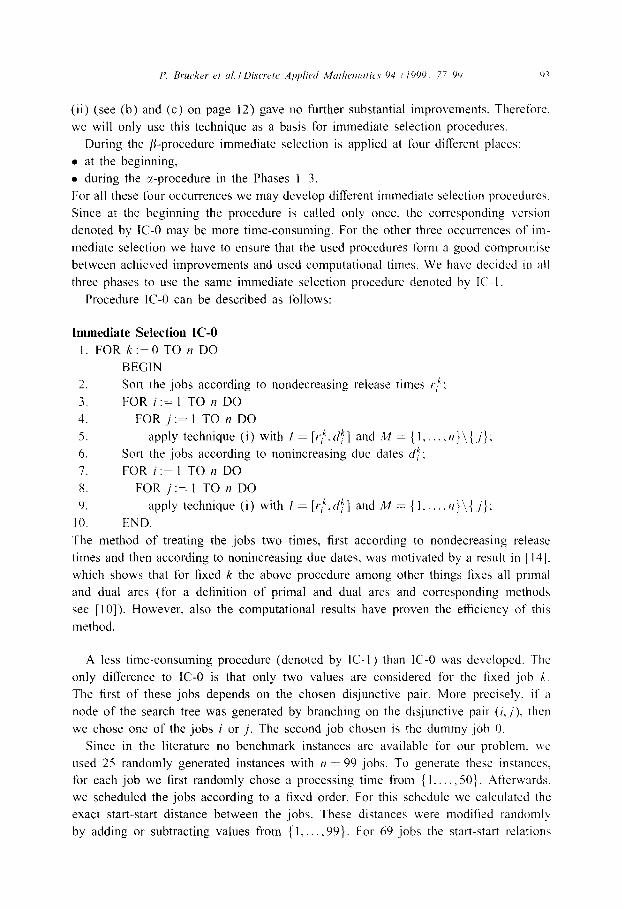
Procedure IC-0 can be described as follows:

Immediate Selection ICY-0

1. FOR k:=O TO n DO

BEGIN

2. Sort the jobs according to nondecreasing release times rj:

3. FORi:=l TOnDO

4. FORj:=l TO n DO

5. apply technique (i) with /=[~:,df] and hl={l,....n}\{,j};

6. Sort the jobs according to nonincreasing due dates df:

7. FORi:=l TOnDO

8. FOR ,j:= 1 TO tz DO

9. apply technique (i) with I = [r/,df] and 1!4 = {I... ..?I}\{ i}:

IO. END.

The method of treating the jobs two times, first according to nondecreasing release

times and then according to nonincreasing due dates, was motivated by a result in [ 141.

which shows that for fixed k the above procedure among other things fixes all primal

and dual arcs (for a definition of primal and dual arcs and corresponding methods

see [IO]). However, also the computational results have proven the efficiency of this

method.

A less time-consuming procedure (denoted by IC-I) than ICY-0 was developed. The

only difference to IC-0 is that only two values are considered for the fixed job X.

The first of these jobs depends on the chosen disjunctive pair. More precisely. if a

node of the search tree was generated by branching on the disjunctive pair (i. j). then

we chose one of the jobs i or j. The second job chosen is the dummy job 0.

Since in the literature no benchmark instances are available for our problem, we

used 25 randomly generated instances with II = 99 jobs. To generate these instances.

for each job we first randomly chose a processing time from { 1.. ,50}. Afterwards.

we scheduled the jobs according to a fixed order. For this schedule we calculated the

exact start-start distance between the jobs. These distances were modified randomly

by adding or subtracting values from { 1.. .99}. For 69 jobs the start-start relations

were defined by these distances, for 10 jobs only by the positive distances (minimal

time-lags), for 10 jobs only by the negative distances (maximal time-lags), and for

10 jobs we defined no start-start relations. Finally, the generated processing times of

the jobs were reduced by multiplying them by factors generated randomly from the

interval [2/3, l] (from a large set of generated instances only such instances which were

feasible and which caused problems for the developed branch and bound procedures

were chosen).

However, even these remaining instances are rather easy. In all but three cases

the optimal value is equal to the initial lower bound. In the remaining three cases the

difference between these two values is only 1 and after the first phase of the fl-procedure

this gap is already closed. The main reason that we nevertheless have computational

times of around 2.5 seconds for these instances is the very large initial interval [LB, UB]

(since these instances are not generated by reductions, only a rather poor upper bound

UB, can be used): Most of the computational time is spent in Phase 1.

To achieve more interesting test instances we have decided to use some of the

reductions from Section 2 (instead of trying to develop more sophisticated generators).

We have reduced benchmark instances for job-shop and open-shop to single-machine

instances with minimal and maximal time-lags. This will result in harder instances with

a different number of jobs. In detail, we considered the following problems:

l Job-shop instances: These instances result from a reduction of job-shop benchmark

instances from Fisher and Thompson [ 131 and from Lawrence [ 181. Our branch and

bound procedure was only able to solve the instance with 6 jobs and 6 machines

from Fisher and Thompson (FTl) and 14 of the 15 instances with 5 machines

from Lawrence (LAO1 ~ LA14) within reasonable time. Additionally, we will give

a result of a run on the famous 10 x 10 instance of Fisher and Thompson (FT2).

The dimensions of the original job-shop problems are given in Table 1.

l Open-shop instarzces: These instances result from a reduction of open-shop bench-

mark problems from Taillard [22] (taiOl-tai40) and Brucker et al. [5] (tai8 l-tai100).

Problems tai9 1~tai 100 (tai8 1 -tai90) are obtained from the instances tai3 1 -tai40 from

Taillard by removing the last (and the second-last) jobs and machines, i.e. by remov-

ing the last (and the second-last) rows and columns. The dimensions of the original

open-shop problems are given in Table 1.

Table I Dimensions of the shop problems

Open-shop problems mxn Job-shop problems

taiO1 ~ tail0

tail I ~ tai20

tai2l ~ tai30

tai81 ~ tai90

tai9l ~ tail00

tai31 - tai40

4x4 FTI 6X6

5X5 FT2 10 X 10 7X7 LAO I -LA05 5x IO 8X8 LA06-LA10 5 x 15 9x9 LAI l-LA14 5 x 20 IO x IO

Table 2

Results for job-shop instances

Problem

FTI

FT2

LAOI-LAOS

LA06m-LAI 0

LAI I -LA I4 .__

LB UB LB-Phase I

707 716 713

22455 22891 22645

10897.2 I1 172.2 ll08Xh

1914X.6 19690.6 19669.6

30117.X 30895.5 30882 0

Optimum

71s

‘2730

I 1093.2

19669.6

3oxx2.0

Table 3

Rewlts for open-shop instances

Problem LB UB LB-Phase I Optimum CPU C‘I’I!-HI -

miOIMail0 246X.7 2674.0 2603.4 2609.0 4.3 0 .I

tai I I- tai20 4027.6 4325.2 4238. 4243.5 252.4 II 1

ta12 I tai30 795 I .4 8416.4 X291.X X291.X 7732.9 X7-l (r

taiX I -tai90 98 13.4 10323.8 10220.5 10220.5 209.1 (8) 1393 (Xt

tai9 I- tai94 12932.0 13548.0 13397.x 13397.x I53 (4) ilOX (\I _ _~___ -_____

Our branch and bound procedure was only able to solve the instance up to 9 jobs

and machines. From the 10 instances with 9 jobs and 9 machines from Bruckel

et al. [ 19951 only the first 4 were solved in reasonable time. Thus, the results of the

remaining 6 instances are not presented.

In Tables 2 and 3 we present the results for the test instances resulting from shop

problems achieved with this branch and bound procedure. The tables contain the thl-

lowing information:

LB: Average value of the initial lower bound.

UB: Average value of the initial upper bound.

LB-Phase I : Average value of the improved lower bound after Phase I.

Optimum: Average optimal value of the instance.

CPU: Average computational time (in s) used by the branch and bound procedure.

CPU-Br: (only Table 3) Average computational time (in s) used by the branch and

bound method B&B,! for the open-shop problem of Brucker et al. [5] on a SC;)\;

SPARC 4/20.

If for the entries CPU or CPU-Br additionally a number is added in parenthesis.

only this number of problems were solved within 50 h.

Contrary to the randomly generated instances, we now have a much smaller initial

interval [LB. UB] and, furthermore, the optimal value is always quite difl’ercnt to the

initial lower bound. However, after the first phase of the /i-procedure the lower bound

has been improved considerably and in many cases was already equal to the optimal

value. A reason for this is that for all these instances special lower bounds on the

job-shop and open-shop also achieve results equal to or nearly equal to the optimal

value (see [5,7]). But in all cases the lower bound after Phase I is not smaller and in

some cases larger than these lower bounds.

96 P. Bucker et al. IDiscrete Applied Muthemutics 94 (1999) 77-99

Table 2 indicates that instances achieved from job-shop can be solved relatively

fast up to 150 single-machine jobs (FTl, LAOl-LAlO). All but one instances are

solved within 5 min and the remaining instance takes 11 min. For the larger instances

(more than 200 jobs) only a few instances could be solved in reasonable time. From

the Lawrence instances of dimension 5 x 20 (leading to instances with 200 jobs)

three were solved within 12 min, one took almost 7 h, and the last (LA15) could not

be solved within 2 days. However, the 10 x 10 instance FTl and the 10 x 10 of

Lawrence (also leading to instances with 200 jobs) could not be solved within 2 days.

For the famous 10 x 10 problem of Fischer and Thompson it took almost 10 days of

computational time to get the optimal solution. This indicates that not only the number

of jobs but especially the structure of the time-lags determine the hardness of instances.

For state-of-the-art branch and bound procedures the instances FTl and LAOl-LA14

are rather easy job-shop instances. They are, e.g. solved by a method of Brucker et al.

[7] using at the most 4s.

For instances resulting from open-shop the border between easy and hard seems to

occur at a smaller number of jobs. We only always get an optimal solution within

7min for instances up to 50 jobs (taiOlMai20). For instances with 98 or 128 jobs

(tai2 lMai30, tai8 I-tai90) only 12 out of 20 instances are solved within 10 min. For

the remaining 8 instances two could not even be solved within 2 days. For the 9 x 9

instances only 4 could be solved quickly, whereas the remaining 6 were not solved

within 2 days. If we compare the computational times of our branch and bound method

for the open-shop problem of Brucker et al. [5] we noticed that our method is much

faster for 3 instances (tai81, tai90, tai91) and for other 3 instances (tai86, tai92, tai93)

comparable with their method (taking into account that the machine used by Brucker

et al. is about 10 times slower). Especially for the larger instances (8 x 8, 9 x 9) the

results of our general branch and bound procedure for the single-machine problem with

minimal and maximal time-lags are rather close to the results of the branch and bound

method designed especially for open-shop problems. The reason that the instances

resulting from open-shop already get harder for a smaller number of jobs may be that

open-shop instances initially have almost no fixed structures (leading to fewer initially

fixed time-lags than for instances resulting from job-shop). This observation is also

responsible for the difficulties in designing efficient branch and bound methods for the

open-shop problem and may explain why our general branch and bound method gets

relatively close to the special branch and bound method for the open-shop problem.

Summarizing, we can state that the branch and bound method designed for the

single-machine problem with arbitrary time-lags leads to satisfactory results for smaller

instances resulting from job-shop and open-shop instances. The results achieved for

the different classes of test instances (randomly generated, reduction from job-shop,

reduction from open-shop) indicate that besides the number of jobs also the structure

of the time-lags determine the hardness of single-machine instances. Whereas for the

first two classes instances with approximately 100 jobs were solved relatively quickly,

instances of this size in the third class caused problems for our branch and bound

method. A closer look at the structure of the instances shows that for instances resulting

from open-shop the relative order is fixed for fewer pairs of jobs than for the randomly

generated instances and instances resulting from job-shop. Since for the ‘missing’ pairs

the branch and bound method has to fix the relative orders, the longer computational

times for the instances resulting from open-shop are not a surprise. On the other hand.

if no or only a few time-lags are given (i.e. for almost no pair the relative order is

fixed), the instances will become easy since many decisions will not be relevant for

finding an optimal solution (many solutions will be optimal).

5. Conclusion

We have shown that complex scheduling problems can be reduced to the prob-

lem of scheduling jobs with arbitrary time-lags given by start-start relations on a

single-machine. The number of jobs and start-start relations used in the single-machine

problem grows at the most quadratically with the number of jobs (operations), ma-

chines, and start-start relations in the original problem. These results are quite sur-

prising. They show that the single-machine problem with start-start relations is a \cry

complex one.

Furthermore. we have presented a branch and bound algorithm for solving the

single-machine problem with arbitrary time-lags. Classical job-shop and open-shop

problems were solved using reductions and this branch and bound algorithm. Hou-

ever, the results show that solution methods for general shop problems which use the

transformation and the branch and bound algorithm for the single-machine problem are

not as efficient as direct methods for general shop problems. This observation likely

also holds for other complex scheduling problems which can be transformed to the

single-machine problem.

Concerning complex scheduling problems with arbitrary time-lags we also deem it

unlikely that the reductions allow to solve them efficiently. A better way would be to

adopt the branch and bound method presented in Section 3 to multi-machine situations.

The transfonnations and the single-machine branch and bound algorithm could be useful

to get some first insight into the multi-machine problems with positive and negative

time-lags. Especially, the concepts of immediate selection and the general ideas of the

branch and bound method could be adapted to multi-machine problems.

There are several further new research directions:

l It is a challenging open problem to find a polynomial reduction from the resource

constraint project scheduling problem to the single-machine problem with arbitrary

time-lags (with the techniques described in Section 2 it is relatively easy to define

a pseudo-polynomial reduction! ).

l The computational results indicate that the hardness of instances depends on the

structure of the time-lags. Is it possible to identify hard instances and. thus. to

generate hard instances randomly’?

l We have only considered problems with C,,, -objective function. Do we get similar

results for other objective functions?

98 P. Bucker et al. I Discrete Applied Muthernatics 94 (1999) 77-99

l When developing the branch and bound algorithm for the single-machine problem

with arbitrary time-lags we incorporated features which can be found in efficient

branch and bound methods for solving shop problems directly. Is it possible to

include promising features from other branch and bound algorithms as well?

l The one-machine instances resulting from the reductions presented in Section 2 natu-

rally decompose into cliques of jobs (associated with the parallel dedicated machines)

which do not overlap in their processing. Thus, concepts of immediate selection may

be applied to each clique separately resulting in a speed-up. Is it possible to derive for

general instances some similar type of decomposition into ‘almost not overlapping’

sets to speed up the immediate selection procedures?

l It seems promising to develop local search heuristics for the single-machine problem

with arbitrary time-lags and to apply these heuristics to other problems using the

reductions.

Acknowledgements

The authors are grateful to the anonymous referees for their helpful comments on

an earlier draft of the paper.

References

[I] M. Bartusch, R.H. Mb;hring, F.J. Rademacher, Scheduling project networks with resource constraints

and time windows, Ann. Oper. Res. I6 (1988) 201-240.

[2] J. Blaiewicz, P. Dell’Olmo, M. Drozdowski, M.G. Speranza, Scheduling multiprocessor tasks on three

dedicated processors, Inform. Processing Lett. 41 (1992) 275-280.

[3] K. Brinkmann, K. Neumann, Heuristic procedures for resource-constrained project scheduling with

minima1 and maxima1 time lags: the minimum project-duration and resource-levelling problems,

J. Decision Systems 5 (I 996) 129-156.

[4] P. Brucker, T. Hilbig, J. Hurink, A Branch & Bound algorithm for scheduling problems with positive

and negative time-lags, Osnabriicker Schriften zur Mathematik, Reihe P, No. 179, 1996.

[5] P. Brncker, J. Hurink, B. Jurisch, B. WGstmann, A branch & bound algorithm for the open shop

problem, Discrete Appl. Math. 76 (1997) 43-59.

[6] P. Brucker, B. Jurisch, A. KrHmer, The job-shop problem and immediate selection, Ann. Oper. Res.

50 (1994) 73-l 14.

[7] P. Brucker, B. Jurisch, B. Sievers, A fast branch & bound algorithm for the job-shop scheduling

problem, Discrete Appl. Math. 49 (1994) 107-127.

[8] P. Brucker, R. Schlie, Job-shop scheduling with multi-purpose machines, Computing 45 (1990)

369-375.

[9] J. Carlier, The one-machine sequencing problem. Eur. J. Oper. Res. I I (1982) 4247.

[lo] J. Carlier, E. Pinson, An algorithm for solving the job-shop problem, Management Sci. 35 (1989)

164-l 76.

[ 1 l] 8. De Reyck, W. Herroelen, A branch-and-bound procedure for the resource-constrained project

scheduling problem with generalized precedence relations, Research Report 9613, Department of Applied Economics, Katholieke Universiteit Leuven, 1996.

[ 121 S.E. Elmaghraby, J. Kamburowski, The analysis of activity networks under generalized precedence

relations, Management Sci. 38 (I 992) 1245-1263.

[ 131 H. Fisher. G.L. Thompson, Probabilistic Icarmng combinations of local job-shop schcduhng rules. in:

J.F. Muth. C.L. Thompson (Eds.). Industrial Scheduling. Prentice-Hall, Englewood Cliffs. N.I. 1963.

pp. 225 -25 I. [ 141 T. Hilbig. Scheduling Probleme mit Start-Start-Relationcn. Diplomarbeit. UmversitIt Ornabriick. I990

1151 1..4. Hoogevecn, S.L. van de Veldt, B. Vcltman, Complexity of scheduling multiprocessor task> \LII~

preapecilicd processor allocation, Disc&c Appl. Math 55 (1994) 259-272.

[ Ih] B. .lurisch. Scheduling jobs in shops with multi-purpose machines, Dissertation. Universitat Owahriick.

1993.

171 U. Klclnau, Zur Struktur und L6sung vcrallyemeincrter Shop-Scheduling-Probleme. Disact-tatIon.

lJnivcrslt% Magdeburg, 1993.

IX] S. Lawrence. Resource constrained prqjcct scheduling: an experimental lnreati~ation of heurl\tlc

scheduling techniques, GSIA. Carnegie Mellon University, 198-l.

191 C.L. Monma, C.N. Potts, On the complexity of schedulin g with batch setup times. Opcr. Kc\ -37

( 1989) 79x-x04.

201 K. Neumann, C. Schwindt. Projects with minimal and maximal tmxz lags: constructIon (11

activity-ownodc networks and applications. Technical Report WIOR-437, lnstltut fir ~~irtschaftstheorlc

und Operatlona Research. University of Karlsruhe. 1995.

211 B. Roy. C‘ontrlbution de la thiorie des graphcb i I’i-tude dc certains probl&x Iln&rca. C’.R. ,\cnd

SCl. 1. 13x. 1959.

221 1:. Taillard. Benchmarks for basic schcdulmg problems, European .lournnl of Operational Rwxrch h-l

(1993) 27x 285.

231 h.D. U’ikum. D.C. Llewellyn. G.L. Nemhauser. One-machine gcneralircd precedcnoe constralncd

scheduling problems. Oper. Res. Lett. I6 (1994) 87-99.

241 .1. /.han. Hcurihtics for scheduling resource-constrained project< in MPM networks. Eur. .I Opel- Rc\

76 ( 1094) 19-205.

2.51 E. Balas, .1.K. Lcnstia, A. Vazacopoulos, The one-machine problem with delayed prccedencc conrtramt<

and I[\ II’IC in job shop scheduling. Management Scicncc 41 ( 1995) 94 109.