a bivariate point process connected with electronic counters

A Bivariate Point Process Connected with Electronic CountersAuthor(s): D. R. Cox and Valerie IshamSource: Proceedings of the Royal Society of London. Series A, Mathematical and PhysicalSciences, Vol. 356, No. 1685 (Aug. 24, 1977), pp. 149-160Published by: The Royal SocietyStable URL: http://www.jstor.org/stable/79374 .

Accessed: 07/05/2014 08:34

Your use of the JSTOR archive indicates your acceptance of the Terms & Conditions of Use, available at .http://www.jstor.org/page/info/about/policies/terms.jsp

.JSTOR is a not-for-profit service that helps scholars, researchers, and students discover, use, and build upon a wide range ofcontent in a trusted digital archive. We use information technology and tools to increase productivity and facilitate new formsof scholarship. For more information about JSTOR, please contact [email protected].

.

The Royal Society is collaborating with JSTOR to digitize, preserve and extend access to Proceedings of theRoyal Society of London. Series A, Mathematical and Physical Sciences.

http://www.jstor.org

This content downloaded from 169.229.32.136 on Wed, 7 May 2014 08:34:32 AMAll use subject to JSTOR Terms and Conditions

http://www.jstor.org/action/showPublisher?publisherCode=rsl

http://www.jstor.org/stable/79374?origin=JSTOR-pdf

http://www.jstor.org/page/info/about/policies/terms.jsp


Proc. R. Soc. Lond. A. 356, 149-160 (1977)

Printed in Great Britain

A bivariate point process connected with electronic counters

BY D. R. Cox, F.R.S. AND VALERIE ISHAM

Department of Mathematics, Imperial College, London

(Received 21 January 1977)

Consider three independent Poisson processes of point events of rates A1, A2 and A12. There are two electronic counters, the first recording events from the first and third Poisson processes, and the second recording events from the second and third Poisson processes. Both counters have constant dead-time, i.e. following the recording of an event on a counter no further event can be recorded on that counter until the appropriate constant time has elapsed. Two ways of estimating A12 are via a coincidence rate, i.e. the rate of occurrence of pairs of events separated by less than a suitable small tolerance, and via the covariance of the numbers of events recorded on the two counters in a suitable time period. The theoretical values of these quantities are calculated allowing for dead-time. The techniques used illustrate the study of bivariate point processes.

1. INTRODUCTION

This paper deals with a counting problem in physics which can be described in general terms as follows. There are two counters and three independent Poisson processes of point events of rates respectively A1, A2 and A12. Events from the first process can be recorded only on the first counter. Events from the second process can be recorded only on the second counter. Events from the third process can be recorded virtually simultaneously on both counters.

This situation is equivalent to one in which there is a single Poisson process of rate A of events, all of which would be counted on both counters were the counters fully efficient. If the counters have efficiencies el and e2, then in the previous formulation

A1 = Ae1(l-62),A2 = Ae2(1-e1) and A12 = Aele2.

Both counters are subject to blocking. Following the recording of an event on the first counter, there is a constant dead-time r1 during which further events cannot be recorded on that counter. Similarly for the second counter there is a constant dead-time r2.

There is an extensive literature on the effect on a single counter of this and more complex forms of blocking (Feller 1948; Smith I958). Here we study aspects connected with the pair of counters, especially those concerned with the estimation of A12. There are in fact two broad techniques for such estimation, namely the counting of coincidences and the estimation of covariances.

For the first method, the sequences of recorded events on the two counters are

6 [149 ] Vol. 356. A. (24 August ,977)



150 D. R. Cox and Valerie Isham

merged and, for some suitable small time span h, a count is made of the number of occasions on which there are two events less than h apart, one from each counter. Note that if h < min (r1, r2) any two events less than h apart must indeed originate from different counters. A value of h is chosen in the light of the 'jitter' in the recording mechanism and of any real displacement between the virtually coincident pairs of events in the third Poisson process. The mathematical problem then is to calculate the rate of occurrence of such coincidences, allowing for counter dead-time and including spurious coincidences.

The second method, which can be used when coincidence techniques are in- applicable for technical reasons, hinges on the fact that for the original Poisson processes, the covariance of the total numbers of events in a time t occurring on the two counters is equal to the variance of the number from the third Poisson process, which in turn is A12t. Therefore, in the absence of blocking, A12 can be estimated via the sample covariance computed from the numbers of events in the two counters as measured in a large number of independent intervals each of length t. The mathematical problem here is to calculate the theoretical value of this covariance for the numbers of events actually recorded, i.e. allowing for dead- time. For further discussion and references and for a semiempirical formula for the covariance, see Lewis, Smith & Williams (I973).

Most of the present paper is devoted to the second problem, the calculation of cov {N1 (t), N2(t)}, where Nl(t) and N2(t) are the numbers of events recorded in time t on counters 1 and 2. In ? 8 we calculate the rate of occurrence of coincidences.

The results may have other applications. The system forms a very special example of a bivariate point process. While the arguments in the paper are entirely rigorous, they have been presented in a way avoiding mathematical technicalities.

2. SOME PRELIMINARY RESULTS

Consider the time interval (0, t) starting from statistical equilibrium. Then

rt NA7(t)= dNft(u) (i = 1,2).

Let Pi = A1 + A12 be the total occurrence rate for the first counter and PI be the equilibrium probability that the counter is open. Then the probability that an event is recorded on that counter in (u, u + Au) is PlPl Au + o(Au). Therefore, E(.) denoting mathematical expectation, we have that

E{N1(t)} = f pr {dNl (u) = 1 = f PlP du = plplt. (1)

Further it follows, by considering the trajectory of the first counter consisting of an alternation of constant dead-times of length -r, with open periods exponentially distributed with mean l/pl, that

Pi = (lIp,)I(lIp ?ri)= (+p1 -r1)-1. (2)



A bivariate point process from electronic counters 151

Similarly for the second counter

E{N2(t)} = p2P2t (3)

with P2 = A2 + A12,p2 (1 +P2r2)-1 To calculate c(t) = cov {Nl(t), N2(t)}, we consider

c(t) = E{Nl(t) N2(t)} - E{N1(t)} E{N2(t)}

= E (f dN(u) dN2(v)}-Pl P2 P1 p2t2 (4)

= f duj dvpr{dN1(u) = dN2(v) - 1}+ dv du o =t+0 0 t=V+0

pr {dN1 (u) = dN2(v) 1}+ ftdupr{dNi(u) = dN2(u) = 1}-PI P2P1P2 t2, (5)

the region of integration in (4) having been split into three parts. Now, formally,

pr {dN,(u) = dN2(v) = 1} = pr {dN1(u) = 1} pr {dN2(v) = 1 i dN1(u) = 1}

=pipLduh12(v-u)dv (v > u), (6)

pr{dN,(u) = dN2(v) = 1} = p2p2dvh21(u -v) du (u > v), (7)

pr{dNL(u) = dN2(u) = 1} = A12P12du. (8)

Here P12 is the equilibrium probability that both counters are open simultaneously, and the second-order cross-intensity functions are defined, for example, by

pr (event recorded on counter 2 in (x, x + Ax) I event

hI2(X) =im Mrecorded on counter 1 at 0)

h Ax-) O + Ax

forx > 0. On substituting (6)-(8) into (5) and taking Laplace transforms, these being

denoted by an asterisk, we have that

c*(s) = Lc(t) e-Stdt

= Pi Pi 1h(s)/s2 +P2P2 h*(s)/82 + A12 P12/s2 -2Pi P2 Pl P2/83s (9)

This shows that in order to find c(t) we need to find P12, the equilibrium probability that both counters are open together, and the two cross-intensity functions.

3. Two COUNTERS AS A MARKOV PROCESS

To study the two counters in more detail, we represent them as a Markov process. For this we must define the state in such a way that the instantaneous transition probabilities are determined by the current state. Thus if a counter is blocked the

6-2




state description must specify for how long the counter has been blocked. The possible states and their equilibrium probabilities or probability densities are as follows:

(i) both counters are open, with probability P12;

(ii) counter 1 has been blocked for time u and counter 2 is open, with probability density q1(u) for 0 < u < -r;

(iii) counter 1 is open and counter 2 has been blocked for time u, with probability density q2(u) for 0 < u < r2;

(iv) counter 1 has been blocked for time u1 and counter 2 for time u2, with probability density q12(u1, u2) for 0 < ui < (i = 1, 2).

For example, the probability that counter 1 is open and counter 2 has been blocked for a time (u, u +Au) is q2(u) Au+ o(Au). Note that there is a non-zero probability that the two counters become blocked simultaneously and that then in case (iv) u1 = U2. It is thus convenient to put

q12(Ul, U2) =qs) (u1) 8(u1 - u2) + qj((u1 u2)j

(10)

where 4(.) is the Dirac delta function and q(C2)(., .) is absolutely continuous. The equilibrium equations of the process can now be obtained; they represent

the balance between the probabilities of entering and leaving a particular state. Throughout the rest of this section and ?? 4 and 5 we deal with the special case of equal counter dead-times, T1- = = r. We write p Al1+ A2 + A12 for the total rate of occurrence of events of all kinds. Then

PP12 = q (T) + q2(T) + q(s)(T),

q, (?) A1 P12, q2(0) = A2 P12, q(s2)(0) = A12 p12, (11)

q(c) 0) P2 q(u), q2)(0, u) = p q2(U);

q'(u)-2q(f = q (j2) (u, -r) (12) q2(u) = -p1q2(U) + q1(j(T, u); J

Dq12(U1, U2)/Du1 +? qI2(u1, U2)/au2 =0. (13)

Finally there is a normalizing condition that the total probability is unity. This system is readily solved. Thus (13) shows that q12(ul, u2) is a function of

l- '62* Therefore we can write q(s)(u) = q2I a constant, and by the last part of (11)

(e)

[P2 q1(ul- u2) (U1

> U2), q12 (U,t2) =

pjq2(u2-U1) (U1 < U2).

Then the equations (12) become

qj(u) +p2q (2)q p1q2(T-U),1 (14)

q2(u) +?pq2(U) = p2q,(T-u).




By examining solutions of the form qi(u) = a exiu, it is easily shown that we must have Xi = -X2 and that Xl(Xl - PI + P2) = O. It can thereby be shown that provided that P, * P2

q1(u) = Ap1 + B e-Plr e(Pl-P2)U, q2(U) = Ap2+Be-P2r e(P2P) U. (15)

We now substitute into ( 1) to find

A = P12 (A1 e T - A2 eP2r) (16) (p1 ePlr-P2 eP2r)

1

B i

A12 P12(P2 - PI) e(Pl+P2) 1 (p, ePl'r- P2 eP2r)

and finally apply the normalizing condition to show that

P12 - PI P2(P1 ePlT -P2 eP2T) (18 (A1 ePlr-A2eP2r)

Note that were the two processes {N1(t)} and {N2(t)} statistically independent, i.e. A12 = 0 and pi = Ai (i = 1, 2), we would have P12 = P1P2* The final factor in (18) expresses the association between the states of the two counters; the factor is strictly greater than unity unless A12 = 0, when the factor is obviously equal to unity. It would be possible to base the estimation of A12 directly on an experi- mental determination of P12.

4. THE CROSS-INTENSITY FUNCTIONS

On the basis of the results of ? 3 we now calculate the cross-intensity function hl2(x). In the definition, the condition that an event is recorded on counter 1 at time 0, implies that counter 1 is open at 0-. Therefore the state of counter 2 at time 0- has the following conditional probabilities:

(i) open, with probability P12/Pl; (ii) closed, having been closed for time u, with probability density q2(U)/pl.

In case (ii), the state of counter 2 is unchanged at time 0 +, but in case (i) there are two possibilities depending on whether the originating event on counter 1 comes from the third or first Poisson processes. Thus at time 0+, we have three possibilities for the state of counter 2, namely:

(i)' just beginning a blocked period, with probability (p12AI2)/(p1pI); (i)" open, with probability (P12A1)/(p1P1); (ii) as above.

For each of these cases the process of recorded events on counter 2 forms a renewal process with the interval between successive events having the density P2 e-P2(X-) (x > T). For (i)', the renewal process is ordinary (i.e. starts with one of the above intervals), in (i)n it is modified by starting with an interval with




exponential density P2 e-P2X (X > 0) and in (ii) it is modified by starting with an interval with density P2 e-P2(x-r+U) (x > - u). It follows that

P12;A12 pA A P1+ P2hx-y h12(x) = 2h(x; T, p2) + P2 eP P2 e x-yT,P2) dy

pip' ip

+p q2(u) h(x + u; T P2) du, (19)

where h(x; , P2) is the ordinary renewal density for process (i)'. Further

hT(s; , P2) P2{(P2 + s) es,- P2-1 (20)

From (19), (20) and (15) we can now calculate the Laplace transform hz (s); in dealing with the last term of (19), note that h(y; T, P2) = (0 < y < T). It follows that

PI 2A1p2 P2 [p22A12 p12AkP2

PIPI(P2 +s) (P2+s) esr P2 L PlPl P1P1(P2 + s)

{ esr-1 A12(p2- p1) ePi 7 (e(s-P1+P2) 1)}] (21 8s (A, ePlr 2eP2r) (8-pl + p2)

with the symmetrical expression for h2*(s).

5. THE COVARIANCE

By substituting (21) and (18) into the formula (9) for the Laplace transform of c(t) = cov {N1(t), N2(t)}, we obtain an explicit expression for c*(s) in our special case

j= 2= -. It is easily shown that c*(s) has a double pole at s = 0 and that the remaining singularities have negative real parts. That is

c*(s) - k/s2 + I/s + c(s), (22)

where cO*(s) is analytic in the half-plane Re (s) > - yo, with yo > 0; in fact elemen-

tary but tedious calculations give

k = A12plp2p12, (23)

21 = 2A122 (PIPi + P2 P2) + 2P1P2A12 P12(P1 eP1-P2 eP2r)-1

x {r2(eP2T - ePlr) (p2 ?p2) + 2(p2 ePlr-p2 eP2r)

+ 2(pl - p2)' (ePl r + eP2 7) (plP + P2P2) + 2T(P, -P2Y1 (pl2 eP2 +p2 eP1 T)

- 2(p, -P2)-2 (eP r- eP2T) (Pl +P2)}. (24)

It can be shown from the explicit form of c*(s) that for large t

c(t) = kt +I+ O(e-yot). (25)

Further, it can be shown that for small T and P2T, TY- - log max (Pi, P2 T) and an asymptotic expansion for yo can be found.




Note that when plr and P2r are both small, P1 P2 and P12 are all near 1, k I* A12, 1-+0 and we recover as a limit the Poisson-based formula c(t) = A12t applying in the absence of counter dead-time. Numerical study and practical use of (25) are helped by noting that for small T

P12 = P1P2{1 + A12r + 0(P)}, 1 = WA12 Pl P2r2(p1p +P2P2) + 0(r3)

If, therefore, we write

c(t) = {A12 p1p 2( + Al2T) t + 2A12 PlP2(P1P2 +P2P ) r2}b(t) (26)

then b(t) will usually be close to one and will vary slowly with the relevant para- meters. Some numerical results are given in ? 7.

Note that the expansions for k and 1, and similar expansions occurring later, could be written in alternative forms, because Pi and P2 are both functions of r. We have used the simplest form in each case.

6. UNEQUAL DEAD-TIMES

Suppose that r1 : r2 and without loss of generality take r1 > T2. Then the equilibrium equations for the Markov process of the counter states are as (11), (12), (13) of ? 3 except that (12) is replaced by

qu q, ( U) + ql2 (uf r2) (27)

q2(u) = p, q2( + q( (Tr, U),

and the first equation in (11) becomes

PP12 = q1(rl)+q2(r2) (28) Thus we must solve

' + {pl~p,q2(T2 -U) (U < 'T2) T

q(uf) = P-2q1(u) + {p2q(-T2) (T2 < U < Ta ), (29)

q2(u) = -p1q2(U)+P2q1(,r-u) (u < r2), J subject to ql(O) = AlP121 q2(0) = A2P12, (30)

where q1 is continuous except for an atom at 2, i.e.

ql(T2+) = ql(T2-)+Al2Pl2. (31) If T1 is an exact multiple of T2 1 = rT2 = rr say, then solution is straightforward. If 5, .., Or are the non-zero roots of

(p1~~)(p+ )r = pipr (32) (P1l 0 (P2 + )1 2 (2 then q1 and q2 have the following forms:

ql(u) AO A+

E A ( ; )e00&f-Pr) \ 2+ (+=i)

(j,r< u <(j +I),r,j=O0, 1... (33)




where Ao, ..., Ar can be obtained by using the continuity of ql(u) at u= 2,..

(r - 1)T, the discontinuity of q1(u) at u = -T given in (31) and the boundary conditions (30). The rermaining unknown P12 can be obtained most simply from

P12+ f duq2(u) = P (34)

To obtain the cross-intensity function h 2(x), the above function q2(u) is sub- stituted into (19). For h21(x) we substitute the above function ql(u) into the symmetrical form of (19), with T replaced by rr.

Finally, using (9), we obtain the Laplace transform of the covariance c(t) and as before we obtain c*(s) - k/s2+ ls + c* (s),

where c*(s) is analytic for Re (s) > -yo, yo > 0. For r 2 we find k = Al2P12PlP2, which has already been shown to hold for r = 1 and in fact holds also when one dead time is zero. We conjecture that the result holds for all T1 and T2, that a direct probabilistic derivation should be possible, and that this should not depend on the relative magnitudes of T1 and T2.

If r > 2 then an exact form for c*(s) may be obtained as described above. Nu- merical solution is complicated because of the roots 5, *-, )r defined in (32), all but two are complex if r is odd and all but three are complex if r is even. However it is straightforward to obtain approximations to q1 and q2 when T is small. For this we make separate Taylor expansions for ql(. ) in the ranges (0, T), (T, 2T), ...

and for q2(.) in the range (0, r) and match coefficients appropriately. If r > 2 we find that

Alp12 + A12(A2 - A1) p12u + 0(T2) (u < r),

q1(u) = P1p2 + A12(A2-A )p12r-p2A12p12(u -) + O(Tr2) (T < u < 2T)

PlP12-piA12p12Tr0(T2) (2T < u <

rT), (35)

q2(u) A2 P12 + P1 A12 P12 UO + 0(T2), (u < r),

and from (34) it follows that

P12 = P1P2(1 + A12r) + O(T2). (36) Then use of (9), together with (19), leads to an approximation to c*(s) of order T2,

fromwhichwe obtain the following generalization of (26) holdingwhen r1 = rT2 = rr:

c(t)-= {A12 p2p2( + A12min ( T2)) t + 2A12 Plr2(PlPl1 +P2 p2T2)} b(t), (37)

where b(t)-1 + 0(T3).

Note that although (35) was derived on the assumption that T1 = r-r2 for some integer r, it is correct for non-integer r at least for r > 3.

Some numerical results are given in ? 7.




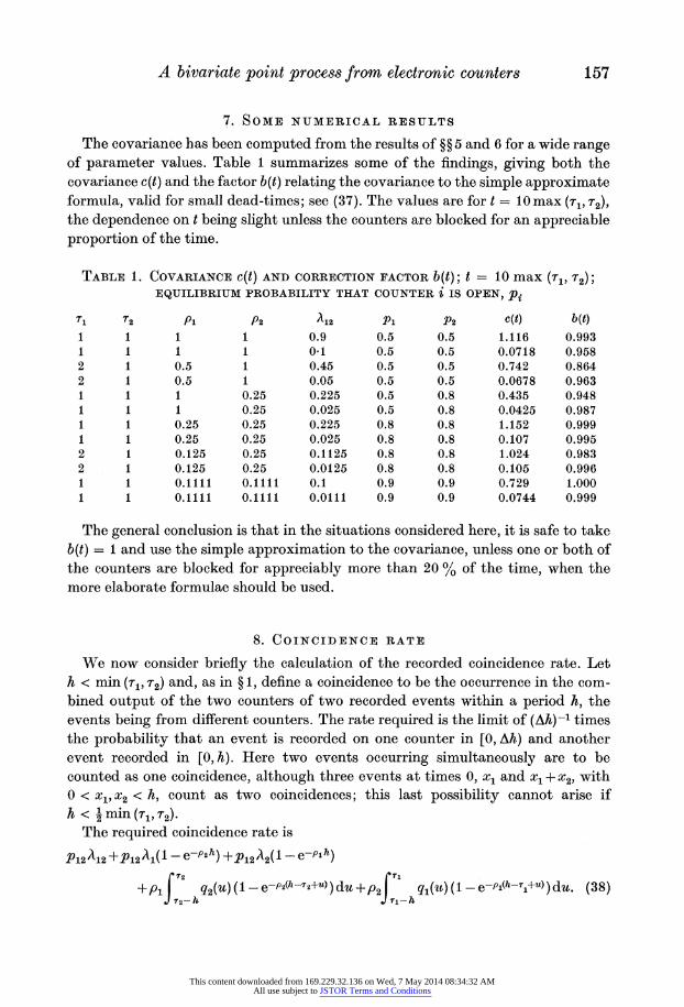
7. SOME NUMERICAL RESULTS

The covariance has been computed from the results of ?? 5 and 6 for a wide range of parameter values. Table 1 summarizes some of the findings, giving both the covariance c(t) and the factor b(t) relating the covariance to the simple approximate formula, valid for small dead-times; see (37). The values are for t = 10 max (T1, l2), the dependence on t being slight unless the counters are blocked for an appreciable proportion of the time.

TABLE 1. COVARIANCE c(t) AND CORRECTION FACTOR b(t); t = 10 max (T1, T2); EQUILIBRIUM PROBABILITY THAT COUNTER i IS OPEN, Pi

T1 T2 Pi P2 A12 Pi P2 c(t) b(t)

1 1 1 1 0.9 0.5 0.5 1.116 0.993 1 1 1 1 0-1 0.5 0.5 0.0718 0.958 2 1 0.5 1 0.45 0.5 0.5 0.742 0.864 2 1 0.5 1 0.05 0.5 0.5 0.0678 0.963 1 1 1 0.25 0.225 0.5 0.8 0.435 0.948 1 1 1 0.25 0.025 0.5 0.8 0.0425 0.987 1 1 0.25 0.25 0.225 0.8 0.8 1.152 0.999 1 1 0.25 0.25 0.025 0.8 0.8 0.107 0.995 2 1 0.125 0.25 0.1125 0.8 0.8 1.024 0.983 2 1 0.125 0.25 0.0125 0.8 0.8 0.105 0.996 1 1 0.1111 0.1111 0.1 0.9 0.9 0.729 1.000 1 1 0.1111 0.1111 0.0111 0.9 0.9 0.0744 0.999

The general conclusion is that in the situations considered here, it is safe to take b(t) = 1 and use the simple approximation to the covariance, unless one or both of the counters are blocked for appreciably more than 20 % of the time, when the more elaborate formulae should be used.

8. COINCIDENCE RATE

We now consider briefly the calculation of the recorded coincidence rate. Let h < min (r1, T2) and, as in ? 1, define a coincidence to be the occurrence in the com- bined output of the two counters of two recorded events within a period h, the events being from different counters. The rate required is the limit of (Ah)-1 times the probability that an event is recorded on one counter in [0, Ah) and another event recorded in [0, h). Here two events occurring simultaneously are to be counted as one coincidence, although three events at times 0, xi and xl + x2, with 0 < xl, x2 < h, count as two coincidences; this last possibility cannot arise if

h<-min (,rl, 2)'

The required coincidence rate is

P12A12 +P12A1(1 - e-P2) +p12A2(1 - e-Plh)

rT2 'rl +P1j q2(u)(1 - e-P2(h-T2+U))du+p2 ql() (-1 e-pj(h-T1+u))du. (38)

T2-h '1-h




Note that, given that a counter, say the first, is open at 0 it can record at most one event in time h. The probability that no event is recorded is e-Pl h, so that the probabilitv of one event is 1 - e-Plh. In (38) the first term represents the genuine coincidence rate A12 deflated by the requirement that both counters must be open in order to record both events; the remaining four terms refer to spurious coincidences.

If ri= 2 = T, it follows by the substitution in (38) of ql(u), q2(U) from (15), that the apparent coincidence rate is

2P1P2 P1P2 h + A12 P12(p, eP,I eh(P2-Pl) -P2 eP2r eh(pl-P2)) 2PIP2PIP2h I(p1,ePlr- p2 eP2r)

(9

If -1 _ rr2 = rT (r > 2), then by using the approximations to q1 and q2 given in (35) it can be shown that the coincidence rate is

2p1p2p12h + A12 P12{ 1 - (Pl

+ P2) h2+ p +p 0(r3), (40)

since h < r. Note that the coincidence rate when r = 1, given by (39), can be written

2P1P2 p12 h + A12 P12{t - (P1 + P2) h + 2(p2 + p2- 2plP2) h2} + 0(T3) (41)

and that (41) is less than (40) by 2P1P2A112P122. As was the case for the covariance, the approximation (40) is valid for non-

integer values of T1/T2 if this ratio exceeds three. It is interesting that to the order given the dead-times T1 and T2 enter only via P12. Bryant (I963) calculated the observed coincidence rate when the counters have equal dead-times. He made in effect the approximation that the functions q1, q2 and q12 are constants, and this is justified only for small dead-times. Further he assumed that the overlap of dead- times caused by noncoincident events is uniformly distributed.

9. SOME EXTENSIONS

We now outline two extensions of the analysis. First it is possible that on one of the counters, say counter 2, there occur events

which cause blocking but which do not contribute to the covariance or coincidence count. Then instead of the original three Poisson processes of rates A1, A2 and A12, we consider five independent Poisson processes of rates A1 (type 1 event only), A2 (type 2 event only), A3 (type 3 event only), A12 (coincident types 1 and 2) and A13 (coincident types 1 and 3). Events of type 3 block counter 2, but do not directly contribute to the covariance or coincidence rate which are those between type I and type 2 events, as before. Assume for simplicity that the dead-times are T1 for counter 1 and T2 for counter 2, the latter applying to both type 2 and type 3 events. Write p = A1 + A12 + A13, P2 = A2 + A12, p3 = A3 + A13.

The previous arguments can be extended, although of course the details get




more complicated. Expansion in powers of T as in (35) gives in the special case

rl =T2, for the covariance between the numbers of type 1 and type 2 events

c(t) = P1P2 p12{A12 + (A12A3 -A13A2) T + O(r3)} t

+ [1p12{A12(p1 + P2) + A13 P2} r2 + 0(r3)] + O(e-yo t), (42)

and for the coincidence rate

P12[A12 + h{2pIp22- A12(P1 + P2) - A13 P2} + 1I&2{A 2(P2-pl)2 + 13p2(p2-Pi)

+P20(3P - A1P3)} + 0(r3)]. (43)

For r1 = 2T2 and i- > 3T2, the coincidence rate exceeds (43) by

fp12h2P1p2(A12 + A13).

Here Pl, P2 and P12 are given exactly by the previous analysis with type 2 and type 3 events merged; in particular P12 is given exactly by (18) with P2 replaced by A2+A3+A12+A13, and A2 by A2+A3.

A second development is to allow for variable counter dead-time for the system with two types of event. Indeed if we make the physically very unrealistic assumption that counter dead-times are independently exponentially distributed with means r1 and T2 the theoretical analysis greatly simplifies, because the Markov process of ? 3 no longer needs the specification of the times for which a counter has been blocked.

The probabilities Pi and P2 that the counters individually are unblocked are still given by (3), but now the probability that both are open is

PiTji+P2T2 (44) P12 =

Tl + 2 + PT, T2'

where p = A1 4 A2 + A12. An equation analogous to (19) holds and simple calculation shows that exactly

c(t) = A12 P12P1P2t + [11 - exp {- t/(p1Tr)}] + 12[1 - exp { - t/(P2T2)}], (45)

where

A12 PT1rlPp2(plTlT2 + T1 + T2) _ A12 P2 2 PiP2(P2T1r2 + T1 + T2) 46 (P7172 + 71 + 72) (P1,T2 + T1 + T2)

The reappearance in (45) of the coefficient of t found in ?? 5 and 6 reinforces the belief that it should be possible to derive the leading term by a simple probabilistic argument.

If r1 = T2 = X, then for small r

P,2 P1P2{1 + wA12r + O(r2)},

so that the approximation to c(t) corresponding to (26) is

c(t) = [A12 p1p (2 + 2A12T) t + A12 P1P2(P1PI +P2 P2) 2] b(t) (47)




The approximation to P12 is smaller for exponential dead-times than for constant dead-times equal to the relevant means; the factor multiplying P1P2 is (1 + AA12r) instead of (1 + A12 r). This is intuitively reasonable since one would expect de- creased association between the counters when the dead-times are random variables. Also the approximation to the constant term in (47) is twice that in (26), suggesting a dependence on mean squared dead-time; for the exponential distribution the mean square is 2T2.

Finally, it would be of practical interest to develop the theory also for the so- called Type II counter, i.e. counter with extended dead-time. In this, events occurring when a counter is blocked, while not recorded, do prolong the dead-time.

We are very grateful to Mr A. Williams and Dr D. Smith, Division of Radiation Science, National Physical Laboratory, for suggesting the investigation and for their advice and encouragement. We thank also Mr N. J. H. Small for computing table 1.

REFERENCES

Bryant, J. I963 Coincidence counting corrections for dead-time loss and accidental coincidences. Int. J. appl. rad. Isotopes 14, 143-151.

Feller, W. 1948 On probability problems in the theory of counters, Courant Anniversary Volume, pp. 105-115.

Lewis, V. E., Smith, D. & Williams, A. I973 Correlation counting applied to the determination of absolute disintegration rates for nuclides with delayed states. Metrologia 9, 14-20.

Smith, W. L. 1958 Renewal theory and its ramifications (with discussion). J. R. statist. Soc. B 20, 243-302.



a bivariate point process connected with electronic counters

Documents