A Biophysical Approach to Production Theory Jing Chen

School of Business University of Northern British Columbia Prince George, BC Canada V2N 4Z9 Phone: 1-250-960-6480 Email: chenj@unbc.ca Web: http://web.unbc.ca/~chenj/

James K. Galbraith Lyndon B. Johnson School of Public Affairs The University of Texas at Austin Austin, TX 78713-8925, USA Phone: 512-471-1244 Email: galbraith@mail.utexas.edu Web: http://www.utexas.edu/lbj/faculty/james-galbraith/

We thank Sufey Chen and participants at Biophysical Economics conference in Syracuse, seminar at University of Texas, Austin and conference on The New Economics as ‘Mainstream’ Economics in Cambridge for helpful comments. All the calculations, graphs and tables in this paper are contained in an Excel file, which can be downloaded at http://web.unbc.ca/~chenj/papers/AnalyticalTheory.xlsx

1

Abstract

Most people agree that human activities are consistent with physical laws. One may naturally think that sensible economic theories can be derived from physical laws and evolutionary principles. This is indeed the case. In this paper, we present a newly developed production theory of economics from biophysical principles. The theory is a compact analytical model that provides, in our view, a much more realistic understanding of economic (as well as social and biological) phenomena than the neoclassical theory of production. It greatly reduces the complexity of our understanding about the economic activities. Keywords: biophysical economics, production theory, fixed cost, variable cost, return

2

1. Introduction Most people agree that human activities are consistent with physical laws. One may naturally think that sensible economic theories can be derived from physical laws and evolutionary principles. This is indeed the case. A newly developed analytical thermodynamic theory of economics provides a much more realistic and intuitive understanding of economic, social and biological phenomena than the mainstream economic theory (Chen, 2005). In this paper, we will present a more detailed discussion of the production theory, which forms one part of the analytical theory. We will show how the new production theory provides a simple and systematic understanding about investment activities and economic policies. There are two fundamental properties of life. First, living organisms need to extract resources from the environment to compensate for the continuous diffusion of resources required to maintain various functions of life. Second, for an organism to be viable, the total cost of extracting resources has to be less than the amount of resources extracted (Odum, 1971, Hall et al, 1986, Rees, 1992). The second property could be understood as natural selection rephrased from the resource perspective. The purpose of our work is to show that a self-contained mathematical theory of production can be derived from these two fundamental properties of life. From the physics perspective, resources can be regarded as low entropy sources (Georgescu-Roegen, 1971). The entropy law states that systems tend toward higher entropy states spontaneously. Living systems, as non-equilibrium systems, need to extract low entropy source from the environment to compensate for their continuous dissipation. It can be represented mathematically by lognormal processes, which contain both a growth term and a dissipation term. According to the entropy law, the thermodynamic dissipation of an organic or economic system is spontaneous. However the extraction of low entropy source from the environment depends on specific biological or institutional structures that incur fixed or maintenance costs. Additional variable cost is also required for resource extraction. Higher fixed cost systems generally have lower variable costs. Fixed cost is largely determined by the genetic structure of an organism or the design of a project. Variable cost is a function of the environment. From the Feynman-Kac formula, a result widely used in science literature, we derive the equation that variable cost of a production system should satisfy. An organism survives if the amount of resources it extracts is higher than the total cost spent. Similarly, a business survives if its revenue is higher than the total cost of production. We set the initial condition of the equation so that total cost is equal to the amount of resource extracted or revenue generated. Then we solve the equation to derive a formula of variable cost as a mathematical function of product value, fixed cost, uncertainty, discount rate and project duration. From this formula of variable cost, together with fixed cost and volume of output, we can compute and analyze the returns and profits of different production systems under various kinds of environment in a simple and systematic way. The results are highly consistent with the empirical evidences obtained from the vast amount of literature in economics and ecology. Furthermore, by putting major factors of production into a compact mathematical model, the theory provides precise

3

insights about the tradeoffs and constraints of various business or evolutionary strategies that are often lost in intuitive thinking. Product value, fixed cost, variable cost, discount rate, uncertainty, project duration and volume of output are major factors in production. These factors naturally became the center of investigation in early economic literature. However, because of the difficulty in forming a compact mathematical model about these factors, discussion about these factors becomes peripheral in current economic literature. With the help of this analytical production theory, theoretical investigation in economics may refocus on important issues in economic activities. Among the various relations of different factors, the relation between fixed cost and variable cost is probably the most important. We will elaborate on this relation further. People observed that useful energy comes from the differential or gradient between two parts of a system. In general, the higher the differential between two parts of a system, the more efficient the work becomes. At the same time, it is more difficult to maintain a system with high differential. In other words, a lower variable cost system requires higher fixed cost to maintain it. This is a general principle. We can list several familiar examples from physics and engineering, biology and economics. In an internal combustion engine, the higher the temperature differential between the combustion chamber and the environment, the higher the efficiency in transforming heat into work. This is the famed Carnot’s Principle, the foundation of thermodynamics. At the same time, it is more expensive to build a combustion chamber that can withstand higher temperature and pressure. Diesel burns at higher temperature than gasoline. This is why the energy efficiency of diesel engine is higher and the cost of building a diesel engine is higher. In electricity transmission, higher voltage will lower heat loss. At the same time, higher voltage transmission systems are more expensive to build and maintain because the distance from the line to the ground has to be longer to reduce the risk of electric shock. The differential of water levels inside and outside a hydro dam generates electricity. The higher the hydro dam, the more electricity can be generated. At the same time, a higher hydro dam is more costly to build and maintain. Warm blooded animals can run faster than cold blooded animals because their body temperature is maintained at high levels to ensure fast biochemical reactions. But the basic metabolism rates of warm blooded animals are much higher than the cold blooded animals. Shops located near high traffic flows generate high sales volume per unit time. But the rent costs in such locations are also higher. Well trained employees work more efficiently. But employee training is costly. The tradeoff between lower variable cost and higher fixed cost is often not explicitly discussed in the same literature. However, the new production theory provides a quantitative measure of return and profit at different levels of fixed cost and variable cost under different kinds of circumstances. From the production theory, it can be calculated that when the fixed cost is zero, the variable cost is equal to the product value. This means that any organisms or organizations need to make fixed investment before earning a positive return. This simple result has broad implications. It means that any viable organization, whether a company or a country, needs

4

a common fixed investment. We will discuss tax policy and the concept of market from the perspective of fixed cost and variable cost further. In current economic literature, taxation is often described as a type of distortion or imperfection. If this is true, any society that abolishes taxation will remove the distortion and become less imperfect. It will crowd out other social systems that collect taxes. However, this has not happened. Montesquieu (1748) observed long ago, “In moderate states, there is a compensation for heavy taxes; it is liberty. In despotic states, there is an equivalent for liberty; it is the modest taxes.” From the mainstream economic theory, we might conclude that despotic states are more perfect than moderate states. In this production theory, tax is considered as a fixed cost of the whole society. Therefore, lower tax rate does not automatically mean a better society. The proper level of taxation should be determined by other factors in the society, such as the general living standard of the population. In neoclassical economics, market is a very abstract concept.

The “market” in modern usage is not some physical location. … The market is the nonstate, and thus it can do everything the state can do but with none of the procedures or rules or limitations. … Because the word lacks any observable, regular, consistent meaning, marvelous powers can be assigned. The market establishes Value. It resolves conflict. It ensures Efficiency in the assignment of each factor of production to its most Valued use. … From each according to Supply, to each according to Demand. The market is thus truly a type of God, “wiser and more powerful than the largest computer,” … Markets achieve effortlessly exactly what governments fail to achieve by directed effort. (Galbraith, 2008, p. 20)

In this production theory, market is a concrete concept. The structure of market is determined by its various parameters. If a market is very small, then its structure will be very simple to reduce fixed cost. If a market is very large, then its structure will be very sophisticated to reduce variable cost. For example, a village market has little formal structure or regulation. But New York stock exchange has very expensive computer systems and highly complex regulatory structures to ensure the smooth flow of large volume of transactions. In this concrete structure, it is meaningless to discuss whether market is “efficient” or not. Any market that turns a positive return will survive and prosper. Any market that turns a negative return will shrink and disappear. For an organism or organization, part of its fixed cost is used to regulate its internal environment to maintain a proper working condition. For example, the human body is regulated at around 37 degree centigrade. When a person is infected, the body temperature is regulated to higher temperature to more effectively attack the infecting bacteria. However, temperature that is too high will damage the brain’s information processing capability, which is sensitive to thermal noises (Gisolfi and Mora, 2000). Hence, regulation is a compromise between different parts of an organism. When a part of an organism escapes regulation and turns into a free market, that part of the organism will grow rapidly.

5

This is called cancer. In the end, the unregulated growth, if it is not stopped, will drain all the resources of the organism and destroy the organism. In human society, if an economic sector gains control of large amount of resources and escapes regulation, it will grow rapidly and generate huge profit for the insiders. But the process will drain resources from the whole society. This is what we have witnessed in the 2007, 2008 financial crisis. Mainstream economists pay little attention to the biophysical foundation of human society because they believe that the special qualities of human beings will make physical constraints less relevant. However, thinking about constraints is a very effective way to understand social phenomena (Galbraith, 2008). A biophysical approach puts the physical constraint of human society at the center of its analysis. The validity of a physical theory of economics is best manifested by the existence of a corresponding mathematical theory that is derived from the most fundamental properties of life and is consistent with a wide range of patterns observed in both economics and ecology. After all, all physical laws are represented by mathematical formulas. By establishing an analytical theory based on biophysical principles, many philosophical and verbal problems can be turned into scientific and quantitative inquiries. The computability of the mathematical theory will transform biological science, which include social science as a special case, into an integral part of physics. This paper is an update from earlier works (Chen, 2005, 2016). It is structured as follows. Section two presents the derivation of the production theory. Section three presents detailed results from this theory. Section four discusses investment decisions in different kinds of environment. Section five explores relations among different parameters that were initially assumed to be independent. Section six concludes. 2. A mathematical theory of production The theory described in this section can be applied to both biological and economic systems. For simplicity of exposition, we will use the language of economics. However the extension to biological system is straight forward. We start the investigation by asking: What are the most fundamental properties of organisms and organizations? How do we represent these fundamental properties in a mathematical theory? First, organisms and organizations need to obtain resources from the environment to compensate for the continuous diffusion of resources required to maintain various functions. This fundamental property can be represented mathematically by lognormal processes, which contain both a growth term and a dissipation term. Suppose S represents the amount of resources accumulated by an organism or the unit price of a commodity, r, the rate of resource extraction or the expected rate of change of price and σ, the rate of diffusion of resources or the rate of volatility of price change. Then the process of S can be represented by the lognormal process

(1) . dzrdtS

dS σ+=

6

where

ondistributiGaussian standard with variablerandom a is 10 , ),N(εdtdz ∈= ε The process (1) is a stochastic process. In this paper, we assume r to be positive and constant. But r can change over time Chen (2010). For example, after a living system dies, r turns negative during its decomposition. Although a stochastic process will generate many different outcomes over time, we are mostly interested in the average outcomes from such processes. For example, although the movement of individual gas molecules is very volatile, air in a room, which consists of many gas molecules, generates a stable pressure and temperature. We usually study the average outcomes of stochastic processes by looking at the averages of the underlying stochastic variables and their functions. These investigations often transform stochastic processes into their corresponding deterministic equations. For example, heat is a random movement of molecules. Yet the heat process is often studied by using heat equations, a type of deterministic partial differential equation. Feynman (1948) developed a method of averaging stochastic processes under very general conditions, which is usually called path integral. Kac (1951) extended Feynman’s method into a mapping between stochastic processes and partial differential equations, which was later known as the Feynman-Kac formula. According to the Feynman-Kac formula (Øksendal, 1998, p. 135), if

(2) ))((),( t

qt SfEeStC −= is the expected value of a function of S at time t discounted at the rate q, then C(t,S) satisfies the following equation

with 𝐶𝐶(0, 𝑆𝑆) = 𝑓𝑓(𝑆𝑆) (4) It should be noted that many functions of S satisfy equation (3). The specific property of a particular function is determined by the initial condition (4). This is similar to the Black-Scholes option theory. The Black-Scholes equation is satisfied by any derivative securities. It is the end condition at contract maturity that determines the specific property of a particular derivative security. Second, for an organism or an organization to be viable, the total cost of extracting resources has to be less than the gain from the amount of resources extracted, or the total cost of operation has to be less than the total revenue. Costs include fixed cost and variable

(3) 21

2

222 qC

SCS

SCrS

tC

−∂∂

+∂∂

=∂∂ σ

7

cost. In general, production factors that last for a long time, such as capital equipment, are considered fixed cost while production factors that last for a short time, such as raw materials, are considered variable costs. If employees are on long term contracts, they may be better understood as fixed costs, although in the economic literature, they are usually classified as variable costs. Typically, a lower variable cost system requires a larger investment in fixed costs, though the converse is not necessarily true. Organisms and organizations can adjust their level of fixed and variable costs to achieve high level of return on their investment. Intuitively, in a large and stable market, firms will invest heavily in fixed cost to reduce variable cost, thus achieving a higher level of economy of scale. In a small or volatile market, firms will invest less in fixed cost to maintain a high level of flexibility. In the following, we will examine the relation between fixed cost and variable cost in a very simple project. Suppose there is a project with a duration that is infinitesimally small. It only has enough time to produce one unit of product. If the fixed cost is lower than the value of the product, in order to avoid arbitrage opportunity, the variable cost should be the difference between the value of the product and the fixed cost. If the fixed cost is higher than the value of this product, there should be no extra variable cost needed for the product. Mathematically, the relation between fixed cost, variable cost and the value of product in this case is the following:

Where S is the value of the product, C is the variable cost and K is the fixed cost of the project. When the duration of a project is of a finite value T, relation (5) can be extended into

as the initial condition for equation (3). Equation (3) with initial condition (6) can be solved to obtain

where

The function N(x) is the cumulative probability distribution function for a standardized normal random variable. From (6), the solution of the equation (3) can be interpreted as the variable cost of the project. However, we will investigate shortly whether the function

)2/()/ln(

)2/()/ln(

1

2

2

2

1

TdT

TrKSd

TTrKSd

σσ

σσ

σ

−=−+

=

++=

(5) )0,max( KSC −=

(6) )0,max(),0( KSSC −=

(7) )()( 21)( dNKedNSeC qTTqr −− −=

8

represented in formula (7) has common properties of variable costs. For a given investment problem, different parties may select different discount rates. To simplify our investigation, we will make the discount rate equal to the expected rate of growth. This is to set 𝑞𝑞 = 𝑟𝑟 (8) This choice of discount rate can be understood from two perspectives. From a biological perspective, fast growing organisms also have a high probability of death. In a steady state, the growth rate has to be equal to the death rate. In the biological literature, the discount rate is usually set equal to the growth rate (Stearns, 1992). From the perspective of economics, in option theory, the discount rate is set equal to the risk free rate. The level of risk of an option contract is represented by implied volatility, which does not necessarily equate with past volatility or future expected volatility. Some people do not agree with the economic logic behind the mathematical derivation of Black-Scholes equation that made the risk related discount rate disappear (Treynor, 1996). However, the disappearance of the separate discount rate greatly simplified our understanding of how option values are related to market variables. From both a biological and economic perspective, this choice of discount rate provides a good starting point for further investigation. With q equals to r, equation (3) becomes

and solution (7) becomes

where

Formula (10) provides an analytical formula of C, variable cost as a function of S, product value, K, fixed cost, σ, uncertainty, T, duration of project and r, discount rate of a firm. Similar to understanding in physics, the calculated variable cost is the average expected cost of variable inputs. With an analytical formula, we can calculate how variable cost changes with respect to other major factors in economic and biological activities. Formula

(9) 21

2

222 rC

SCS

SCrS

tC

−∂∂

+∂∂

=∂∂ σ

(10) )()( 21 dNKedSNC rT−−=

)2/()/ln(

)2/()/ln(

1

2

2

2

1

TdT

TrKSd

TTrKSd

σσ

σσ

σ

−=−+

=

++=

9

(10) takes the same form as the Black-Scholes formula for European call options. But the meanings of the parameters in this theory differ from that in the option theory. We will briefly examine the properties of formula (10) as a representation of variable cost. First, the variable cost is always less than the value of the product when the fixed cost is positive. No one will invest in a project if the expected variable cost is higher than the product value. Second, when the fixed cost is zero, the expected variable cost is equal to the value of the product. When the fixed cost approaches zero, the expected variable cost will approach the value of the product. This means that businesses need to make a fixed investment before they can expect a profit. Similarly, all organisms need to invest in a fixed structure before they can extract resources profitably. Some do not agree with this statement and provide examples of low fixed cost investment with high profits, such as J. K. Rowling writing Harry Potter books. Our results are about the statistical average. While a small percentage of authors earn high incomes from blockbusters, an average author does not earn a high income. Third, when fixed costs, K, are higher, variable costs, C, are lower. Fourth, for the same amount of the fixed cost, when the duration of a project, T, is longer, the variable cost is higher. This shows that investment value depreciates with time. Fifth, when risk, σ, increases, the variable cost increases. Sixth, when the discount rate becomes lower, the variable cost decreases. This is due to the lower cost of borrowing. All these properties are consistent with our intuitive understanding of and empirical patterns in production processes. After obtaining the formula for the variable cost in production, we can calculate the expected profit and rate of return of an investment. Suppose the volume of output during the project life is Q, which is bound by production capacity or market size. During the project life, we assume the present value of the product to be S and the variable cost to be C. Then the total present value of the product and the total cost of production are

respectively. The net present value of the project is

𝑄𝑄𝑆𝑆 − (𝑄𝑄𝐶𝐶 + 𝐾𝐾) = 𝑄𝑄(𝑆𝑆 − 𝐶𝐶) − 𝐾𝐾 (12) The rate of return of this project can be represented by

It is often convenient to represent S as the value of output from a project over one unit of time. If the project lasts for T units of time, the net present value of the project is

(11) and KCQSQ +

(13) 1- )( QCK

QSQCK

QCKQS+

=++−

10

(14) )()( KCSTKTCTS −−=+−

The rate of return of this project can be represented by

Unlike a conceptual framework, this mathematical theory enables us to make quantitative calculations of returns of different projects under different kinds of environments. Since our theory is very similar to Black-Scholes option theory, it is essential to compare the basic equations of Black-Scholes theory and our theory. The Black-Scholes equation is

The basic equation in our theory is

The Black-Scholes equation has a negative sign in front of the time derivative. From the physics perspective, our equation represents a thermodynamic process while the Black-Scholes equation represents a reverse thermodynamic process. From the economic perspective, Black-Scholes equation solves the current price of derivative securities when the future payout is determined while our equation solves the expected variable cost in the future when the current fixed cost is determined. These two theories solve different problems in economic activities. In the next several sections, we will provide more detailed analysis on the relation of various factors and returns.

3. Basic properties of the theory This theory provides quantitative measurements about how major factors in economic and biological systems affect costs and returns of the systems. In the following, we will present some of the calculations

(15) 1- )( TCK

TSTCK

TCKTS+

=++−

(16) 21

2

222 rC

SCS

SCrS

tC

−∂∂

+∂∂

=∂∂

− σ

(9) 21

2

222 rC

SCS

SCrS

tC

−∂∂

+∂∂

=∂∂ σ

11

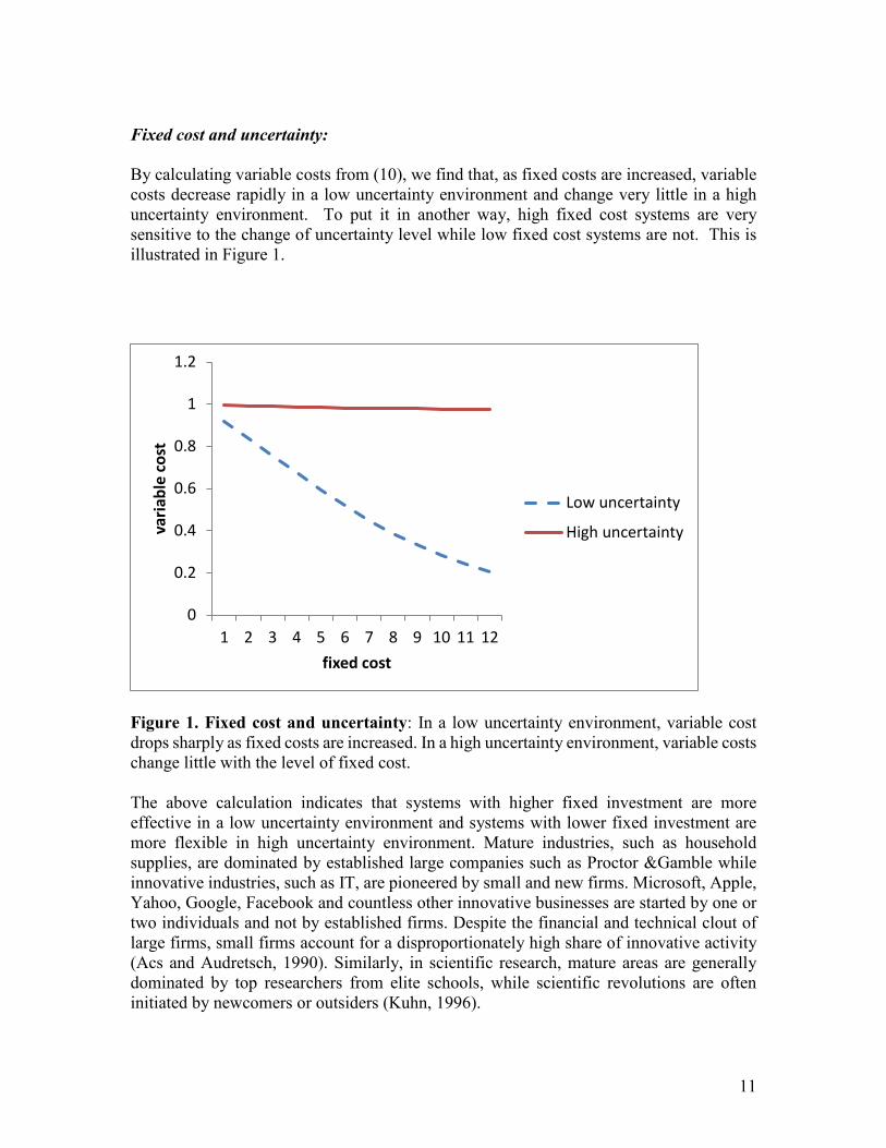
Fixed cost and uncertainty: By calculating variable costs from (10), we find that, as fixed costs are increased, variable costs decrease rapidly in a low uncertainty environment and change very little in a high uncertainty environment. To put it in another way, high fixed cost systems are very sensitive to the change of uncertainty level while low fixed cost systems are not. This is illustrated in Figure 1.

Figure 1. Fixed cost and uncertainty: In a low uncertainty environment, variable cost drops sharply as fixed costs are increased. In a high uncertainty environment, variable costs change little with the level of fixed cost. The above calculation indicates that systems with higher fixed investment are more effective in a low uncertainty environment and systems with lower fixed investment are more flexible in high uncertainty environment. Mature industries, such as household supplies, are dominated by established large companies such as Proctor &Gamble while innovative industries, such as IT, are pioneered by small and new firms. Microsoft, Apple, Yahoo, Google, Facebook and countless other innovative businesses are started by one or two individuals and not by established firms. Despite the financial and technical clout of large firms, small firms account for a disproportionately high share of innovative activity (Acs and Audretsch, 1990). Similarly, in scientific research, mature areas are generally dominated by top researchers from elite schools, while scientific revolutions are often initiated by newcomers or outsiders (Kuhn, 1996).

0

0.2

0.4

0.6

0.8

1

1.2

1 2 3 4 5 6 7 8 9 10 11 12

varia

ble

cost

fixed cost

Low uncertainty

High uncertainty

12

Figure 2. Fixed cost and the volume of output: For a high fixed cost investment, the breakeven market size is higher and the return curve is steeper. The opposite is true for a low fixed cost investment. Fixed cost and the volume of output or market size: We now discuss the returns of investment on projects of different fixed costs with respect to the volume of output or market size. Figure 2 is the graphic representation of (14) for different levels of fixed costs. In general, higher fixed cost projects need higher output volume to breakeven. At the same time, higher fixed cost projects, which have lower variable costs in production, earn higher rates of return in large markets. We can see from the above discussion that the proper level of fixed investment in a project depends on the expectation of the level of uncertainty and the size of the market. When the outlook is stable and the market size is large, projects with high fixed investment earn higher rates of return. When the outlook is uncertain or market size is small, projects with low fixed cost break even more quickly. In the ecological system, the market size can be understood as the size of resource base. When resources are abundant, an ecological system can support large, complex organisms (Colinvaux, 1978). Physicists and biologists are often puzzled by the apparent tendency for biological systems to form complex structures, which seems to contradict the second law of thermodynamics (Schneider and Sagan, 2005; Rubí, 2008). However, once we realize that systems of higher fixed cost provide higher return in the resource rich and stable

-0.4

-0.3

-0.2

-0.1

0

0.1

0.2

0.3

0.4

3 4 5 6 7 8 9 10 11 12 13

Rate

of r

etur

n

Volume of output

Low fixed cost

High fixed cost

13

environments, this evolutionary pattern becomes easy to understand. An example from physiology will highlight the tradeoff between fixed and variable cost with different levels of output.

An increased oxygen capacity of the blood, caused by the presence of a respiratory pigment, reduces the volume of blood that must be pumped to supply oxygen to the tissues. …The higher the oxygen capacity of the blood, the less volume needs to be pumped. There is a trade-off here between the cost of providing the respiratory pigment and the cost of pumping, and the question is, Which strategy pays best? It seems that for highly active animals a high oxygen capacity is most important; for slow and sluggish animals it may be more economical to avoid a heavy investment in the synthesis of high concentrations of a respiratory pigment. (Schmidt-Nielson, 1997, p. 120)

This is another example of fixed cost, variable cost trade-off. For high output systems (highly active animals) investment is fixed cost (respiratory pigment) is favored while for low output systems (slow and sluggish animals) high variable cost (more pumping) is preferred. Pumping is variable cost compared with respiratory pigment because respiratory pigment lasts much longer. With the volatile commodity market, people become aware of the problem of resource depletion. Many people have advocated the increase of efficiency as a way of reduce energy consumption. Will the increase of efficiency reduce overall resource consumption? Jevons made the following observation more than one hundred years ago.

It is credibly stated, too, that a manufacturer often spends no more in fuel where it is dear than where it is cheap. But persons will commit a great oversight here if they overlook the cost of improved and complicated engine, is higher than that of a simple one. The question is one of capital against current expenditure. … It is wholly a confusion of ideas to suppose that the economic use of fuel is equivalent to the diminished consumption. The very contrary is the truth. As a rule, new modes of economy will lead to an increase of consumption according to a principle recognized in many parallel instances. (Jevons, 1865 (1965), p. xxxv and p. 140)

Put it in another way, the improvement of technology is to achieve lower variable cost at the expense of higher fixed cost. Since it takes larger output for higher fixed cost systems to breakeven, to earn a positive return for higher fixed cost systems, the total use of energy has to be higher than before. That is, technology advancement in energy efficiency will increase the total energy consumption. Jevons’ statement has stood the test of time. Indeed, the total consumption of energy has kept growing, almost uninterrupted decades after decades, in the last several centuries, along with the continuous efficiency gain of the energy conversion (Inhaber, 1997; Smil, 2003; Hall, 2004). Take hybrid cars as an example. Hybrid cars have two engines, one internal combustion engine, like conventional cars and one electric engine. This adds to the manufacturing cost (and hence resource consumption) of hybrid cars. If the owner of a hybrid car drives very

14

little, the total resource consumption from a hybrid car is actually higher than a conventional car. Only when a hybrid car is used extensively, it becomes less wasteful relative to a conventional car. Therefore, the use of a hybrid car, when manufacturing cost is included, guarantees high resource consumption. Fixed cost and return We will examine how different level of fixed cost investment will affect the value of a project. From Figure 3, as the fixed cost of a project is increased, the net present value of the project will increase initially. When the level of fixed cost is at certain level, its further increase will reduce the value of the project. Eventually the value of the project will become negative if its fixed cost is too high. Education is a type of fixed cost in our life. We generally regard education a worthwhile investment. But the majority of people will not pursue Ph.D. degrees.

Figure 3. Fixed cost and return: Duration of the project and return We will study how the level of the duration of projects affects its return. If the duration of a project is too short, we may not be able to recoup the fixed cost invested in the project. If the duration of a project is too long, the variable cost, or the maintenance cost may become too high. With the mathematical theory, we can make quantitative calculations. The detailed calculation is illustrated in Figure 4. Its shape is very similar to Figure 3. From Figure 4, as the lifespan of a project is increased, the net present value of the project will increase initially. When the lifespan is at certain level, its further increase will reduce the value of the project. Eventually the value of the project will become negative if its lifespan is too high. It explains why individual life does not go on forever. Instead, it is of higher

-2-1.5

-1-0.5

00.5

11.5

22.5

33.5

1 2 3 4 5 6 7 8 9 10

NPV

Fixed cost

15

return for animals to have finite life span and produce offspring. This also explains why most businesses fail in the end (Ormerod, 2005).

Figure 4. Duration and return Calculation also shows that when the level of fixed cost increases, the length of duration for a project to earn a positive return also increases. This suggests that large animals and large projects, which have higher fixed cost, often have longer life. There is an empirical regularity that animals of larger sizes generally live longer (Whitfield, 2006). The relation between fixed cost and duration can be also applied to human relation. In child bearing, women spend much more effort than men. Therefore we would expect women value long term relation while men often seek short term relation, which is indeed the case most of the time (Pinker, 1997). Since higher fixed cost systems have longer life span than lower fixed cost systems, the mutation rates of lower fixed cost systems are faster. This gives lower fixed cost systems advantages in adapting changes. For example, AIDS virus is much smaller than human beings and can mutate much faster. This makes it difficult for humans to develop natural immune response or develop drugs to fight against AIDS virus. However, higher animals develop a general strategy in immunes systems that has been very effective most of the time. Instead of developing one kind of antibody, our immune systems produce millions of different types of antibodies. It is highly likely that for any kind of bacteria or viruses, there is a suitable antibody to destroy them. This strategy is very effective but very expensive, because our body needs to produce many different kinds of antibodies that are useless most of the time. When we are too young, too old or too weak, our bodies don’t have enough energy to produce large amount of antibodies. That is when we get sick often.

-6-5-4-3-2-1012345

5 10 15 20 25 30 35 40 45 50NPV

Duration

16

From calculation, when the duration of a project keep increasing, the return of a project will eventually turn negative. Hence, duration of a project or an organism cannot become infinite. For life to continue, there has to be a systematic ways to generate new organisms from old organisms. From earlier calculation, for a system to have a positive return, fixed assets have to be invested first. Thus old generations have to transfer part of their resources to younger generations as the seed capital before younger generations can maintain positive return. Therefore, there is a universal necessity of resource transfer from the old generation to the younger generation in biological world. “Higher” animals, such as mammals, generally provide more investment to each child than “lower” animals, such as fish. In human societies, parents provide their children for some years before they become financial independent. In general, wealthy societies provide more investment to children before they start to compete in the market than poor societies. In businesses, new projects are heavily subsidized at their beginning stages by cash flows from profitable mature projects. Since project life or organism life cannot last forever, resource transfer from organism to organism or from project to project is unavoidable. However, the process of transfer is often the source of many conflicts. Businesses prefer lower tax rates. Educational institutions prefer higher government revenues. Each child wants more attention from parents. Parents would like to distribute resources more or less evenly among different children. Mature industries, which need little R&D expense, prefer low tax systems. High tech industries, which rely heavily on universities to provide new technologies, employees and users, strongly advocate government support in new technologies. In good times, financial institutions preach the virtue of free market to pursue high profits. In bad times, the same institutions will remind the public how government support can ensure financial stability of the nation. The amount of resource transfer and the method of resource transfer often define the characteristics of a species or a society. Fixed cost and discount rate: We discuss how the level of fixed cost affects the preference for discount rates. We will calculate how variable costs change with different discount rates. When discount rates are decreased, the variable costs of high fixed cost systems decrease faster than the variable costs of low fixed cost systems (Figure 5). This indicates that high fixed cost systems have more incentive to maintain low discount rates or lending rates. This result helps us understand why prevailing lending rates are different at different areas or times.

17

Figure 5. Fixed cost and discount rate: When discount rates are decreased, variable costs of high fixed cost systems decreases faster than variable costs of low fixed cost systems. In poor countries, lending rates are very high; in wealthy countries, lending rates charged by regular financial institutions, other than unsecured personal loans, such as credit card debts, are generally very low. To maintain a low level of lending rates, many credit and legal agencies are needed to inform and enforce, which is very costly. As wealthy countries are of high fixed cost, they are willing to put up the high cost of credit and legal agencies because the efficiency gain from lower lending rate is higher in high fixed cost systems. In the last several hundred years, there is in general an upward trend in living standard worldwide. There is also a downward trend in interest rates (Newell and Pizer, 2003). Empirical investigations show that the human mind intuitively understands the relation between discount rate and different level of assets. In the field of human psychology, there is an empirical regularity called the “magnitude effect” (small outcomes are discounted more than large ones). Most studies that vary outcome size have found that large outcomes are discounted at a lower rate than small ones. In Thaler’s (1981) study, respondents were, on average, indifferent between $15 immediately and $60 in a year, $250 immediately and $350 in a year, and $3000 immediately and $4,000 in a year, implying discount rates of 139%, 34% and 29%, respectively. Since the human mind is an adaptation to the needs of survival and reproduction, evaluating the relation between discount rate and amount of investment must be a common task in our evolutionary past. Differences in fixed costs in child bearing between women and men also affect the differences in discount rates between them. Women spend much more effort in child bearing. From our theory, the high fixed investment women put in child bearing would make women’s discount rate lower than men’s. An informal survey conducted in a class showed that discount rates of the female students are lower than that of the male students.

0

0.2

0.4

0.6

0.8

1

1.2

0.5 0.45 0.4 0.35 0.3 0.25 0.2 0.15 0.1 0.05 0

varia

ble

cost

discount rate

18

Our understanding about discount rate and fixed cost is similar to an earlier work by Ainslie and Herrnstein (1981):

The biological value of a low discount rate is limited by its requiring the organism to detect which one of all the events occurring over a preceding period of hours or days led to a particular reinforcer. As the discounting rate falls, the informational load increases. Without substantial discounting, a reinforcer would act with nearly full force not only on the behaviors that immediately preceded it, but also on those that had been emitted in past hours or days. The task of factoring out which behaviors had actually led to reward could exceed the information processing capacity of a species.

Discount rate and project duration: When the discount rate becomes lower, the variable cost of a project will decrease and profit will increase. Projects with different lengths of duration will be affected differently from the reduction of discount rates. Figure 6 presents the ratios of profits between projects at low and high discount rates at different levels of project duration. As project lengths are increased, the ratios mostly increase as well. This indicates that projects with longer duration benefit more from the reduction of interest rates. Keynes made a similar argument that as interest increases, the optimal duration of production process shortened (Keynes, 1936, p. 216).

Figure 6. Project duration and discount rate: the ratios of profits between projects at low and high discount rates at different levels of project duration

00.20.40.60.8

11.21.41.61.8

0 2 4 6 8 10 12

Ratio

of p

rofit

s

Duration of projects

19

Next we calculate the breakeven point of a project with respect to the project duration and the discount rate. Let us assume that project output per unit of time is one. The calculation from formula (14) shows that it requires lower discount rate to breakeven when the project duration is lengthened. The calculation results are illustrated in Figure 7. Many empirical studies have documented that humans, as well as other animals, often discount long duration events at lower rates than short duration events (Frederick, Loewenstein and O’Donoghue, 2004). This pattern is called hyperbolic discounting. The calculation provides a possible explanation for hyperbolic discounting. Since it takes lower discount rates for long duration projects to breakeven, human and other animals minds will discount long duration projects with lower rates.

Figure 7. Required discount rate for the project to break even at different project duration: As project duration increases, required discount rate for the project to break even decreased. This provides a possible explanation for hyperbolic discounting. In the following, we will present more empirical evidences about the inverse relationship between discount rate and duration of project or span of life. Fecundity, as well as mortality rate, is proximity for discount rate (Stearns, 1992). Lane (2002) provided a detailed discussion about the tradeoff between longevity and fecundity in the biological systems.

Notwithstanding difficulties in specifying the maximum lifespan and reproductive potential of animals in the wild, or even in zoos, the answer is an unequivocal yes. With a few exceptions, usually explicable by particular circumstances, there is indeed a strong inverse relationship between fecundity and maximum lifespan. Mice, for example, start breeding at about six weeks old, produce many litters a year, and live for about three years. Domestic cats start breeding at about one year, produce two or three litters annually, and live for about 15 to 20 years. Herbivores usually have one offspring a year and live for 30 to 40 years. The implication is that high fecundity has a cost in terms of survival, and conversely, that investing in long-term survival reduces fecundity.

-0.05

0

0.05

0.1

0.15

0.2

0.25

0.3

0 20 40 60 80

Disc

ount

rate

Duration

20

Do factors that increase lifespan decrease fecundity? There are number of indications that they do. Calorie restriction, for example, in which animals are fed a balanced low-calorie diet, usually increase maximum life span by 30 to 50 per cent, and lower fecundity during the period of dietary restriction. … The rationale in the wild seems clear enough: if food is scarce, unrestrained breeding would threaten the lives of parents as well as offspring. Calorie restriction simulates mild starvation and increase stress-resistance in general. Animals that survive the famine are restored to normal fecundity in times of plenty. But then, if the evolved response to famine is to put life on hold until times of plenty, we would expect to find an inverse relationship between fecundity and survival. (Lane, 2002, p. 229)

Lane went on to provide many more examples on the inverse relation between longevity and fecundity. In human society, we often use longevity, or duration of human life as an indicator of the quality of a social environment. At the same time, societies that enjoy a long life span, such as Japan, are often concerned about below replacement fertility. Intuitively, the aging population needs a great amount of resources to maintain their health, which reduces the amount of resources available to support children. Hence, there is a natural tradeoff between longevity and fertility. This result has important policy implications on the balance between resource distribution on longevity and fertility. In a society with below replacement fertility, this poses a great challenge to maintain a sustainable society. Discount rate and uncertainty Variable cost is an increasing function of discount rate. When uncertainty is low, variable cost is much lower with a low level of discount rate. When uncertainty is high, variable costs are not very sensitive to discount rate. Therefore, it is often more effective to reduce discount rate in a stable environment. Figure 8 presents the change of variable costs at different levels of discount rates when levels of uncertainty are low and high. It shows that the reduction of the variable cost is more significant at a low uncertainty level. This explains why r species, which have high discount rates, often thrive in highly uncertain environments. It may show why low interest rates, in a climate of economic crisis, have little effect on the level of perceived profitability and therefore on activity. This is called “pushing on a string.”

21

Figure 8. Change of variable costs with discount rate at different levels of uncertainty The same idea about the relationship between discount rate and uncertainty had been reached earlier. “The same discount curve that is optimally steep for an organism’s intelligence in a poorly predictable environment will make him unnecessarily shortsighted in a more predictable environment (Ainslie, 1992, p. 86).

4. Decision making in different kinds of environment

Decision makers will attempt to maximize the value or return of an investment in any given environment. Very often, the levels of discount rate and uncertainty are external environmental factors not controlled by businesses. People may choose the level of fixed cost and lifespan of projects to maximize the value or return of a project in that specific environment. For brevity, we will assume decision makers maximize value of a project in the following discussion. Environment of different discount rates Let discount rate take two different values at 3% and 10% per annum respectively and keep the level of uncertainty same. We will choose the level of fixed cost and lifespan of the project to maximize formula (14), the net present value of the project. The left side of Table 1 lists the maximization result.

discount rate 0.03 0.1 0.03 0.1

annual output 1 1 1 1

0

0.2

0.4

0.6

0.8

1

1.2

0.22 0.2 0.18 0.16 0.14 0.12 0.1 0.08 0.06 0.04 0.02

varia

ble

cost

discount rate

22

Fixed cost 7.1 3.9 7.1 3.9

duration of project 35.7 13.6 35.7 13.6

uncertainty 0.3 0.3 0.8 0.8

variable cost 0.46 0.42 0.97 0.86

NPV 12.3 4.0 -6.2 -2.0

Table 1. From Table 1, we find that when interest rate is lower, the amount of fixed investment is larger, investment duration is longer and the net present value is higher. So investors normally prefer low interest rate environment. However, the net present values are expected returns calculated at the beginning of a project. The actual returns depend on future environment. Suppose after the projects are built, the actual level of uncertainty becomes 80% per annum instead of 30% per annum as previously expected. We can recalculate the net present values from (14) to find the net present value of the first project, built in the low interest rate environment of 3%, becomes -6.2 billion dollars while the net present value of the second project, built in the high interest rate environment of 10%, becomes -2.0 billion dollars. The right side of the above table lists the calculated results in the new environment. Both projects suffer losses. But the first project suffers much more losses. When environmental conditions change, values of investment in low interest rate environment experience larger fluctuations. In other words, the monetary policy of low interest rate will generate greater business cycles. So business cycles are greatly tied to monetary policies. This theory provides a simple and clear understanding about the level of interest rate and magnitude of business cycles. Stability is destabilizing Hyman Minsky once said, “Stability is destabilizing”. What does it mean exactly? With an analytical theory, we can obtain a very clear understanding from an example similar to the one at the beginning of this section. Suppose in two countries A and B, annual output is 1 billion dollars. Suppose interest rate is 5% per annum in both countries. Uncertainty rate is 30% per annum in country A and 55% per annum in country B. Decision makers attempt to maximize the net present value of investment project. How much will be the desired fixed costs and how long will the expected project last? What are the net present values of projects in countries A and B? We attempt to maximize (14), which is net present value of an investment by changing fixed cost, K and duration, T when uncertainty rates are set at 30% and 55% per annum respectively. Left side of Table 2 lists the calculated results. uncertainty 0.3 0.55 0.8 0.8 annual output 1 1 1 1

23

Fixed cost 5.8 2.1 5.8 2.1 discount rate 0.05 0.05 0.05 0.05 duration of project 25.3 12.1 25.3 12.1 variable cost 0.44 0.64 0.94 0.82

NPV 8.5 2.3 -4.4 0.0

Table 2. From Table 2, we find that when uncertainty rate is lower, the amount of fixed investment is larger, investment duration is longer and the net present value is higher. So investors normally prefer low uncertainty rate environment. However, the net present values are only expected returns calculated at the beginning of a project. The actual returns depend on future environment. Suppose after the projects are built, the actual level of uncertainty becomes 80% per annum in both countries due to circumstances unforeseen by decision makers, such as a global financial crisis. We recalculate (14) to find the new net present values. The net present value of the first project, built in the low uncertainty rate environment of 30%, is -4.4 billion dollars while the net present value of the second project, built in the high uncertainty rate environment of 55%, is 0.0 billion dollars. The calculated results are listed at the right side of Table 2. The first project suffers heavy losses while the second project barely breaks even. When environmental conditions change dramatically, values of investment in formerly stable environment experience large fluctuations. In other words, “Stability is destabilizing”. With this analytical theory, simulation is very simple. It enables us to perceive long term consequences of economic policies and social structures clearly. This theory provides a simple and clear understanding of monetary policies and business cycles. Detailed discussion on monetary policy and business cycles is presented in Chen (2012, 2016). Many economists and policymakers do sense the long term implications of their policies. However, without a simple tool to communicate the long term impacts, most people naturally focus their attention to short term outcomes.

5. Relations among parameters So far, we have assumed the parameters in the production processes, fixed cost, duration of the project, discount rate, uncertainty and quantity of output, to be independent variables. But in reality, these parameters often have complex and varying relations. It takes detailed knowledge and deep insight about each system to model these relations well. In the following, we will present some simple attempts to model such relations. All parameters in our theory, except uncertainty, correspond to directly observable quantities. This is very similar to option pricing theory, in which all parameters, except volatility, correspond to directly observable quantities. In option pricing theory, volatility

24

is often called implied volatility because volatility is implied from the option prices. Similarly in our theory, uncertainty is implied from the expected variable costs. Indeed, the value of uncertainty can involve many factors. The meaning of uncertainty rate can be very different in different applications. Economy of scale and the law of diminishing return All economic systems experience economy of scale and the law of diminishing return at the same time. This can be modelled by setting uncertainty as a function of output. This can be modeled with uncertainty, σ, as an increasing function of the volume of the output. Specifically, we can assume lQ+= 0σσ Where σ0 is the base level of uncertainty, Q is the volume of output and l> 0 is a coefficient. Intuitively, when the size of a company increases and the business expands, the internal coordination and external marketing becomes more complex. With the new assumption, we can calculate the rate of return of production from formula (13). The result from the calculation is presented in Figure 9. From Figure 9, the rate of return initially increases with the production scale, which is well known as the economy of scale (Romer, 1986). When the size of the output increases further, the rate of return begin to decline. This is the law of diminishing return. In specific applications, we can analyze how each factor influence the shape of return curves and try to obtain high rate of returns for our investment.

Figure 9. Volume of output and the rate of return: The rate of return of a project with respect to volume of output, when uncertainty is an increasing function of volume of output

-0.01

0

0.01

0.02

0.03

0.04

0.05

0.06

0.07

20 30 40 50 60 70 80 90 100 110 120 130 140

Retu

rn

Output

25

Increasing fixed cost to reduce uncertainty When the fixed cost of a system increases, the increased fixed cost can often help reduce uncertainty. Many organisms, from stegosaurus to turtles, invest in armor to decrease predation. Air conditioning and heating systems can reduce the uncertainty of temperature in a building. But air conditioning requires an increase in electricity consumption. Insurance can reduce uncertainty of large losses for the policyholders. Yet, insurance premium needs to be paid. This pattern can be modeled with uncertainty, σ, as a decreasing function of the fixed cost. Specifically, we can assume lKe−+= 0σσ where σ0 is the base level of uncertainty, K is the fixed cost and l> 0 is a coefficient. Assume the unit product value is 1, discount rate is 5% per annum, duration of project is 10 years. Assume σ0 is 20% per annum and l is 0.2. Calculated rate of return from the project with different levels of fixed cost is shown in Figure 10. When the level of fixed cost is increased, the rate of return increases initially and then declines. Many decision makings involve the spending of fixed cost to reduce uncertainty, such as unemployment insurance, old age insurance, medical insurance, and governments’ guarantee to financial institutions. People often take polar positions in debating these issues. A good quantitative model will help us reach compromise among various parties.

Figure 10. Increasing fixed cost to reduce uncertainty, showing the relation between level of fixed cost investment and rate of return Resource abundance and investment decisions

0

0.02

0.04

0.06

0.08

0.1

0.12

0.14

3 4 5 6 7 8 9

retu

rn

fixed cost

26

One way to represent the resource abundance and quality is by the level of uncertainty rate. In physics, the term representing uncertainty rate in lognormal process is often called the diffusion rate, or the dissipation rate. A higher dissipation rate means that more energy is wasted as heat and less energy is applied to do useful work, indicating low quality of energy fuels. For example, when a dry cell gets discharged, its internal resistance gradually increases and more energy turns into unusable heat. The quality of the dry cell declines over time. So the quality of resources can be represented by the (inverse of the) uncertainty rate, or dissipation rate. In the following, we will apply the analytical theory to understand how the cost of processing natural resources affects the structure and size of economic systems. We will model the increase of processing costs for natural resources through the increase of diffusion rate. From the calculation of (10), when the diffusion rate is higher, the variable cost becomes higher. Intuitively, higher diffusion rates mean more effort is needed to process the same amount of resources. Specifically, the level of diffusion will be modelled as: lQ+= 0σσ

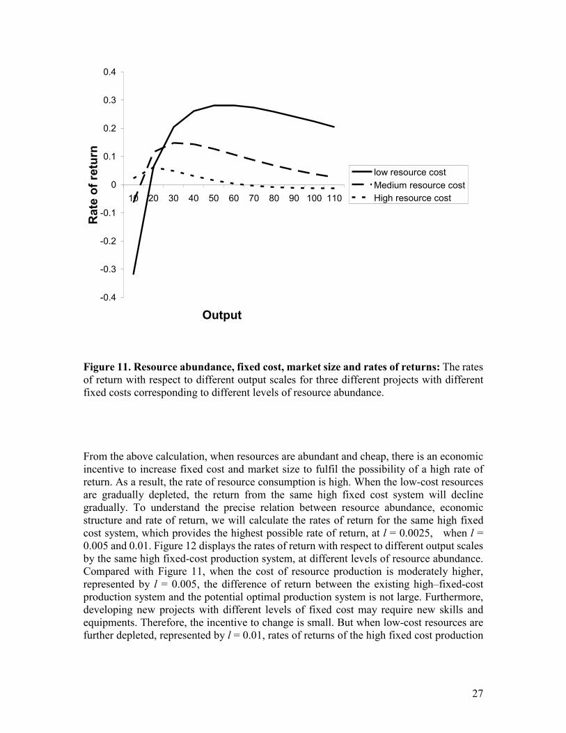
σ0 is the base level of diffusion, which corresponds to the lowest cost in production when resource of highest quality is used. Q is the total output of economy and l > 0 is a coefficient. The size of l represents the abundance of low cost resources. When a low-cost resource is abundant, l is small. An increase of output will not increase processing costs substantially. When the low-cost resource is scarce, l is large. An increase of output will require high-cost resources, which increases the processing cost substantially. We will examine how changes in resource abundance affect the structure of and return on economic activity. For simplicity, we will set S =1, r = 0.1, T =15 and σ0 = 0.4. We will let l take the values of 0.0025, 0.005 and 0.01 to represent different levels of resource abundance. By maximizing formula (13) with respect to the fixed cost and volume of output at different values of l, we obtain the highest possible rate of return from investment projects in different environments. When l = 0.0025, projects obtain the highest possible rate of return of 28% when the fixed cost is 9.5 and market size is 56. When l = 0.005, projects obtain the highest possible rate of return of 15% when fixed cost is 4.5 and market size is 33. When l = 0.01, projects obtain highest possible rate of return of 6% when the fixed cost is 1.7 and market size is 20. Figure 11 displays the rates of return with respect to different sizes of output by three different projects with different fixed costs corresponding to different levels of resource abundance.

27

Figure 11. Resource abundance, fixed cost, market size and rates of returns: The rates of return with respect to different output scales for three different projects with different fixed costs corresponding to different levels of resource abundance. From the above calculation, when resources are abundant and cheap, there is an economic incentive to increase fixed cost and market size to fulfil the possibility of a high rate of return. As a result, the rate of resource consumption is high. When the low-cost resources are gradually depleted, the return from the same high fixed cost system will decline gradually. To understand the precise relation between resource abundance, economic structure and rate of return, we will calculate the rates of return for the same high fixed cost system, which provides the highest possible rate of return, at l = 0.0025, when l = 0.005 and 0.01. Figure 12 displays the rates of return with respect to different output scales by the same high fixed-cost production system, at different levels of resource abundance. Compared with Figure 11, when the cost of resource production is moderately higher, represented by l = 0.005, the difference of return between the existing high–fixed-cost production system and the potential optimal production system is not large. Furthermore, developing new projects with different levels of fixed cost may require new skills and equipments. Therefore, the incentive to change is small. But when low-cost resources are further depleted, represented by l = 0.01, rates of returns of the high fixed cost production

-0.4

-0.3

-0.2

-0.1

0

0.1

0.2

0.3

0.4

10 20 30 40 50 60 70 80 90 100 110

Output

Rat

e of

retu

rn

low resource cost Medium resource cost High resource cost

28

system turn negative at all levels of output, as shown in Figure 12. Reduction of fixed cost and output size are then required to restore economic activities to positive returns.

Figure 12. Resource abundance and rates of returns: The rates of return with respect to different output scales for the same high-fixed-cost production system corresponding to different levels of resource abundance. Since it takes a long time and great effort to adjust institutional structures, it will be very helpful to estimate the state of resource abundance today and in the near future. In a now classic paper titled The End of Cheap Oil, Campbell and Laherrere (1998), after carefully examining the data on oil exploration and production, concluded “What our society does face, and soon, is the end of the abundant and cheap oil on which all industrial nations depend.”

6. Concluding Remarks

Many pioneering works apply physical and evolutionary ideas to economic theory. These works generally use ordinary differential equations to describe economic activities (Chen, 1987). As biophysical and economic activities are thermodynamic processes, we expect thermodynamic equations, which are partial differential equations, describe economic activities more accurately. In this paper, we present an analytical theory of production by solving a thermodynamic equation. The generality of this theory is a consequence from

-0.5

-0.4

-0.3

-0.2

-0.1

0

0.1

0.2

0.3

0.4

1 2 3 4 5 6 7 8 9 10 11

Market size

Rat

e of

retu

rn

Low resource costMedium resource costHigh resource cost

29

the generality of physical laws. Physical systems, biological systems and economic systems all follow the same physical laws. This allows us to develop a unified production theory that can be applied to many different fields. Historically, some economic type principles in physics, such as principle of least action and maximum entropy principle (Jaynes, 1957), have been very fruitful in providing unified foundations to very diverse areas of investigation. The production theory presented in this work has provided a unified understanding for a wide range of problems in economics and biology. Since the theory was developed, it has been applied to project investment, corporate finance, trade and migration, resource and social structures, language and cultures, evolutionary and institutional economics, fiscal and monetary policies, business cycles, firm size and competitions, software development economics and many other problems ( Chen, 2016; Chen and Choi, 2009; Chen and Galbraith, 2011, 2012a, 2012b; Liu, Kong, Chen, 2015). There are more detailed relations among these major factors in specific systems. Some relations are explored in this paper. However, much work needs to be done to provide a more accurate and detailed understanding of the economic and social behaviors.

30

Reference

Acs, Z. and Audretsch D. 1990. Innovation and Small Firms. Cambridge: MIT Press

Ainslie, George, 1992, Picoeconomics: The Interaction of Successive Motivational States within the Person, Cambridge University Press Ainslie, George and Herrnstein, Richard, 1981, Preference Reversal and Delayed Reinforcement, Animal Learning and Behavior, 9, 476-482. Aoki, Masanao and Yoshikawa, Hiroshi, 2006 Reconstructing Macroeconomics: A Perspective from Statistical Physics and Combinatorial Stochastic Cambridge University Press Arnott, R. and Casscells, A. 2003. Demographics and Capital Market Returns, Financial Analysts Journal, 59, Issue 2, p. 20-29. Beck, K. and Andres, C. 2002. Extreme Programming Explained : Embrace Change, 2nd Edition, Addison-Wesley Black, F. and Scholes, M. 1973. The Pricing of Options and Corporate Liabilities, Journal of Political Economy, 81, 637-659. Chen, J. 2005. The physical foundation of economics: An analytical thermodynamic theory, World Scientific, Hackensack, NJ Chen, J. 2006a. An Analytical Theory of Project Investment: A Comparison with Real Option Theory, International Journal of Managerial Finance, 2, No. 4, p. 354-363 Chen, J. 2006b. Imperfect Market or Imperfect Theory: A Unified Analytical Theory of Production and Capital Structure of Firms, Corporate Finance Review, 11, No. 3, 19- 30 Chen, J. 2008. Ecological Economics: An Analytical Thermodynamic Theory, in Creating Sustainability Within Our Midst, edited by Robert Chapman, Pace University Press, 99-116. Chen, J. 2012. The Nature of Discounting, Structural Change and Economic Dynamics, Vol. 23, p. 313-324. Chen, J. 2016. The Unity of Science and Economics: A New Foundation of Economic Theory, Springer.

31

Chen, J. and Choi, S. 2009. Internal firm structure, external market condition and competitive dynamics, Global Business and Economics Review, Vol. 11, No.1. 88 – 98. Chen, J. and Galbraith, J. 2011.Institutional Structures and Policies in an Environment of Increasingly Scarce and Expensive Resources: A Fixed Cost Perspective, Journal of Economic Issues, Vol 45, No 2, 301-308. Chen, J. and Galbraith, J. 2012a. Austerity and Fraud under Different Structures of Technology and Resource Abundance, Cambridge Journal of Economics, Vol. 36, Issue 1, 335-343. Chen, J. and Galbraith, J. 2012b. A Common Framework for Evolutionary and Institutional Economics, Journal of Economic Issues, Vol. 46 Issue 2, 419-428, Chen, P. 1987. Origin of the Division of Labour and a Stochastic Mechanism of Differentiation. European Journal of Operational Research, 30(3), pp.246-250. Chen, P. 2010. Micro interaction, meso foundation, and macro vitality: Essays on complex evolutionary economics. London: Routledge Clark, William, 2008, In Defense of Self: How the Immune System Really Works, Oxford University Press.

Colinvaux, P. 1978. Why big fierce animals are rare: an ecologist’s perspective. Princeton: Princeton University.

D’Arista, Jane, 2009, Setting an agenda for monetary reform, Working paper. Dixit, A. and Pindyck, R. 1994. Investment under uncertainty, Princeton University Press, Princeton. Feynman, R. 1948. Space-time approach to non-relativistic quantum mechanics, Review of Modern Physics, Vol. 20, p. 367-387.

Feynman, R and Hibbs, A. 1965. Quantum mechanics and path integrals, McGraw-Hill. Frederick, S., Loewenstein, G., and O’Donoghue, T., 2004. Time discounting and time preference: A critical review, in Advances in Behavioral Economics, edited by Camerer, C., Lowenstein, G. and Rabin, M., Princeton University Press.

Galbraith, James, 2008. The Predator State: How Conservatives Abandoned the Free Market and Why Liberals Should Too, Free Press Galbraith, J. 2014. The End of Normal: The Great Crisis and the Future of Growth, Simon & Schuster

32

Georgescu-Roegen, N. 1971. The entropy law and the economic process. Harvard University Press, Cambridge, Mass. Gisolfi, Carl and Mora, Francisco, 2000, The hot brain: survival, temperature, and the human body, Cambridge, Mass., MIT Press. Hall, C., Cutler J. C., Robert K., 1986. Energy and Resource Quality: The Ecology of the Economic Process, John Wiley & Sons. Inhaber, H. 1997 Why energy conservation fails, Quorum Books, Westport, Connecticut

Jablonka, Eva and Lamb, Marion J. 2006 Evolution in Four Dimensions: Genetic, Epigenetic, Behavioral, and Symbolic Variation in the History of Life, The MIT Press Jaynes ET. 1957, Information Theory and Statistical Mechanics. Physical Review, 106:

620-630 Jevons, W. 1871. The theory of political economy. London: Macmillan and Co. Jevons, William Stanley, 1865, The Coal Question: An Inquiry Concerning the Progress of the Nation, and the Probable Exhaustion of Our Coal-Mines London: Macmillan and Co Kac, M. 1951. On some connections between probability theory and differential and integral equations, in: Proceedings of the second Berkeley symposium on probability and statistics, ed. by J. Neyman, University of California, Berkeley, 189--215. Kac, M. 1985. Enigmas of Chance: An Autobiography, Harper and Row, New York. Keynes, J.M., 1932, Essays in persuasion, Harcourt, Brace and Company, New York. Keynes, J. M. 1936. The general theory of money, interest and employment Kuhn, T. 1996. The structure of scientific revolutions, 3rd edition. University of Chicago Press, Chicago. Liu, L. Kong, X. Chen, J. (2015). How Project Duration, Upfront Costs And Uncertainty Interact And Impact On Software Development Productivity? A Simulation Approach, International Journal of Agile Systems and Management, Vol. 8, No. 1, p. 39-52 Lane, Nick, 2002, Oxygen: The Molecule that Made the World, Oxford University Press Mehrling, P., 2005. Fischer Black and the Revolutionary Idea of Finance, Wiley.

33

Moalem, Sharon and Prince, Jonathan, 2008, Survival of the Sickest: The Surprising Connections Between Disease and Longevity, Harper Perennial Montesquieu, Baron de, 1748 [1949]. The spirit of Laws, trans. Thomas Nugent, New York. Newell, Richard and Pizer, William, 2003, Discounting the distant future: how much do uncertain rates increase valuations? Journal of Environmental Economics and Management, Volume 46, Issue 1, 52-71. Odum, H.T. 1971. Environment, Power and Society, John Wiley, New York. Øksendal, B. 1998. Stochastic differential equations: an introduction with applications, 5th edition. Springer , Berlin ; New York . Ormerod, P. 2005. Why most things fail, Evolution, extinction and economics, Faber and Faber, London. Pinker, S. 1997. How the mind works, W. W. Norton. New York. Rando, Oliver J. and Verstrepen, Kevin J., 2007, Timescales of Genetic and Epigenetic Inheritance, Cell, Volume 128, Issue 4, 655-668 Rees, William. 1992. "Ecological footprints and appropriated carrying capacity: what urban economics leaves out". Environment and Urbanisation 4 (2): 121–130 Romer, P.M., 1986. Increasing returns and long-run growth. Journal of political economy, 94(5), pp.1002-1037. Rubí, J. Miguel, 2008, The Long Arm of the Second Law, Scientific American; Vol. 299 Issue 5, p62-67 Rushton, P. 1996. Race, evolution, and behavior: a life history perspective, New Brunswick, NJ: Transaction Publishers. Schmidt-Nielson, Knut, 1997, Animal Physiology, fifth edition, Cambridge University Press. Schneider E. D. and Sagan, D., 2005. Into the cool: energy flow, thermodynamics, and life, Chicago: University of Chicago Press. Smil, Vaclav, 2003 Energy at the Crossroads: Global perspectives and uncertainties, The MIT Press, Cambridge, MA.

34

Stearns, S. 1992. The evolution of life histories, Oxford University Press, Oxford. Stiglitz, Joseph, 2002, Globalization and its Discontents, W.W. Norton & Company. Thaler, R. 1981. Some empirical evidence on dynamic inconsistency, Economics Letters, 8(3), 201-207 Treynor, Jack, 1996, Remembering Fischer Black, Journal of Portfolio Management, Vol. 23, December, p. 92-95. Whitfield, J., 2006, In the Beat of a Heart: Life, Energy, and the Unity of Nature, Joseph Henry Press.