A biofuel mandate and a low carbon fuel standard with ‘double

counting’

Johanna Jussila Hammes – VTI

CTS Working Paper 2014:19

Abstract European Union’s (EU) energy legislation from 2009 is still being implemented in the

Member States. We study analytically the Renewable Energy Directive and the Fuel

Quality Directive’s provisions for the transport sector. The former Directive imposes a

biofuel mandate and allows double counting of some biofuels. The latter Directive

imposes a Low Carbon Fuel Standard (LCFS). We show that either the biofuel

mandate or the LCFS is redundant. Double counting makes the biofuel mandate easier

to fulfil but also depresses the price of biofuels. Production of the doubly counted

biofuels increases nevertheless and production of the single-counted biofuels falls.

Given the type of technical change studied, double counting spurs technical

development of the doubly counted biofuels. The LCFS directs support towards those

biofuels with lowest life-cycle carbon emissions. The redundant policy instrument, the

biofuel mandate or the LCFS, only creates costs but no benefits and should be

abolished. Double counting makes the biofuel mandate non-cost-efficient and should

be reconsidered.

Keywords: biofuel mandate; low carbon fuel standard; double counting; technical change;

European energy legislation JEL Codes: D61, H21, H23

Centre for Transport Studies SE-100 44 Stockholm Sweden www.cts.kth.se

1

A biofuel mandate and a low carbon fuel standard with ‘double counting’

Author: Johanna Jussila Hammes a, b

a Swedish National Road and Transport Research Institute, VTI; Box 55685; 102 15

Stockholm, Sweden. E-mail: johanna.jussila.hammes@vti.se. Tel: 00-46-8-555 77 035.

b Centre for Transport Studies Stockholm, CTS; Teknikringen 10A; 114 28 Stockholm,

Sweden.

Abstract: European Union’s (EU) energy legislation from 2009 is still being implemented

in the Member States. We study analytically the Renewable Energy Directive and the Fuel

Quality Directive’s provisions for the transport sector. The former Directive imposes a

biofuel mandate and allows double counting of some biofuels. The latter Directive

imposes a Low Carbon Fuel Standard (LCFS). We show that either the biofuel mandate or

the LCFS is redundant. Double counting makes the biofuel mandate easier to fulfil but

also depresses the price of biofuels. Production of the doubly counted biofuels increases

nevertheless and production of the single-counted biofuels falls. Given the type of

technical change studied, double counting spurs technical development of the doubly

counted biofuels. The LCFS directs support towards those biofuels with lowest life-cycle

carbon emissions. The redundant policy instrument, the biofuel mandate or the LCFS,

only creates costs but no benefits and should be abolished. Double counting makes the

biofuel mandate non-cost-efficient and should be reconsidered.

Keywords: biofuel mandate; low carbon fuel standard; double counting; technical change;

European energy legislation

2

Abbreviations: EU – European Union; FQD – the Fuel Quality Directive; LCFS – Low

Carbon Fuel Standard; RED – the Renewable Energy Directive;

3

1 Introduction

While negotiations to shape the European Union’s (EU) climate- and energy policy

framework post 2020 are already underway, the legislation enacted in 2009 is still being

implemented at the Member State level. An example is the biofuel mandate that Sweden

implements from May 1st 2014 (Jussila Hammes, 2014). EU legislation is complex, and

several parts of the policy package should be analysed together, along with an analysis of

the possible consequences of domestic legislation. The present paper concentrates on

legislation for the transport sector.

EU policy has several goals. The main ones mentioned in the introduction to Directive

2009/28/EC (the Renewable Energy Directive, RED) are to ‘reduce greenhouse gas

emissions and comply with the Kyoto Protocol to the United Nations Framework

Convention on Climate Change… [to] promot[e] the security of energy supply, [to]

promot[e] technological development and innovation, and [to] provid[e] opportunities for

employment and regional development, especially in rural and isolated areas’ (point 1,

introduction to Directive 2009/28/EC). The introduction to Directive 2009/30/EC (the

Fuel Quality Directive, FQD) mentions some additional goals as reasons for regulating the

quality of petrol and diesel fuels, namely health and environment, including air quality

and the need to reduce greenhouse gas emissions.

The policy instrument imposed by the RED on transport sector is a biofuel mandate. This

sets a goal of 10 % of energy use from renewable sources in the transport sector by year

2020. The Directive’s Article 21(2) stipulates that certain biofuels can be counted twice

towards the fulfilment of the national targets. These include biofuels produced from

4

wastes, residues, non-food cellulosic material and ligno-cellulosic material. For the most

part, these are biofuels that are not yet commercially viable (Swedish Energy Agency,

2009, p. 60). The double-counting provision is motivated by the need to support

technological development (point 87, introduction to Directive 2009/28/EC).

To be eligible to be counted towards the biofuel mandate, biofuels have to fulfil the

‘sustainability criteria’ also included in the RED. Thus, biofuels should not be derived

from biomass grown on land with rich biodiversity and high carbon stock. The

sustainability criteria also set a minimum greenhouse gas reduction threshold of 50 % in

2017 for biofuels (Article 17(2), Directive 2009/28/EC; Baral, 2009).

Besides the RED, even the Fuel Quality Directive (FQD) (2009/30/EC) too affects the

consumption of biofuels. Its Article 7a requires fuel suppliers to ‘reduce… life cycle

greenhouse gas emissions per unit of energy from fuel and energy supplied by up to 10 %

by 31 December 2020, compared with the fuel baseline standard…’. Only 6 % of the

reduction is binding, however.1 This policy constitutes a Low Carbon Fuel Standard

(LCFS).

1 2 % of the optional reduction is attained from the implementation of carbon capture and storage

technologies and the remaining 2 % from clean development mechanism credits, above all from reductions

in the greenhouse gas intensity of fossil fuels, which can be realised from reduced flaring and venting of

natural gas in conjunction with oil production (see

http://ec.europa.eu/clima/policies/transport/fuel/index_en.htm; Baral, 2009).

5

Consumption of renewable transport fuels has grown over the past ten years, that is, even

before the EU enacted its 2009 legislation. Figure 1 shows the share of renewable energy

in transport for the average of 28 EU countries and some selected Member States for the

period from 2004 to 2012; this is the period for which data from Eurostat is available. The

overall trend in biofuel consumption over the period has been upwards, year 2011 being

the exception. We have no information about what might have caused the break in the

trend in 2011.

In this paper we study a biofuel mandate based on the RED and a LCFS based on the

FQD. We discuss how double counting affects the policies, how they are affected by

technological change that lowers production costs, and how the EU policy functions when

coupled with three possible national-level policy instruments: fuel tax and/or CO2 tax

exemptions, feed-in tariffs and tradable biofuel certificates. The paper leaves out some

important aspects, including the impact of border taxes and international trade in fuels and

their feedstocks. We do not consider the impact of EU’s energy efficiency legislation.

Furthermore, we do not evaluate either the optimal level of policy instruments,

internalization of the relevant external effects, or do a welfare economic analysis of

policy. Even questions pertaining to uncertainty are left outside the paper’s remit.

This paper is disposed of as follows: Section 2.1 discusses some literature studying biofuel

policy and LCFSs. In Section 2.2 we set up a simple model of the fuel market and

examine the design of a biofuel mandate (2.3), a LCFS (2.4), and the interplay between

these two (2.5). Section 3 uses the model to examine how double counting functions with

a biofuel mandate (3.1) and a LCFS (3.2), the impact of technological change on the two

6

policy instruments (3.3) and finally, three possible national-level policy instruments that

could be used by the EU Member States to implement the EU legislation nationally: fuel

tax exemptions (3.4.1), feed-in tariffs (3.4.2) and tradable biofuel certificates (3.4.3). The

last section concludes.

2 Methods

This section starts with a short literature overview. We then proceed to model the fuel

market and the policy instruments of interest: a biofuel mandate and a LCFS and the

interplay between these two.

2.1 Literature

An active research field dealing with policy instruments for biofuels examines the

interplay between trade policy and domestic biofuel policies such as blending (biofuel)

mandates (Le Roy et al. 2011; Eggert and Greaker, 2012), biofuel subsidies

(Bandyopadhyay, et al., 2013), and tax credits (Crago & Khanna, 2009). Le Roy et al.

(2011) show that import restrictions directly undermine the effectiveness and increase the

costliness of a higher consumption mandate in Canada. Eggert and Greaker (2012) note

that the optimal border carbon adjustment depends on the domestic subsidy to biofuels

production in the presence of a suboptimally implemented blending mandate, High levels

of subsidies may actually imply that a negative border carbon adjustment is optimal.

Bandyopadhyay et al. (2013) show that a second-best biofuel subsidy is positive

(negative) for a large food exporting (importing) country, while the results for a small

country are inconclusive. Crago and Khanna (2009) find that the optimal tax on fuel is

7

directly related to their greenhouse gas emissions intensity while the optimal tariff is

inversely related to the excess supply elasticity of imported ethanol.

De Gorter and Just (2009) analyse the economics of a blend mandate for biofuels in

conjunction with a tax rebate on biofuels. They show that a combination of a biofuel

mandate and a tax rebate constitutes a subsidy to general fuel use but does not give any

direct support to biofuels. Cui et al. (2011) show that a second best policy of a fuel tax and

ethanol subsidy in the US approximate fairly closely the welfare gains associated with the

first best policy of an optimal carbon tax and tariffs on traded goods. Conditional on the

current fuel tax, an optimal ethanol mandate is superior to an optimal ethanol subsidy.

Jussila Hammes (2014) analyses the Swedish biofuel quota system, its winners and losers,

and proposes an alternative. The Swedish system is characterized by three separate quotas,

two for different types of biodiesel and one for biofuels that can be blended in gasoline.

The alternative she suggests is a system with tradable biofuel certificates. Greaker et al.

(2012) examine whether a renewable fuel standard, taking the non-renewable character of

fossil fuels and indirect land use changes into account, actually reduces greenhouse gas

emissions. They find that at least in the short run, given that the emissions from biofuels

are sufficiently low, the renewable fuel standard reduces total fuel consumption and

consequently the climate costs from fuel consumption.

A first economic analysis of the LCFS was made by Holland et al. (2008). Their model

shows that even though a LCFS lowers the production of high-carbon fuels, since it

increases the production of low-carbon fuels, the net effect may be an increase in carbon

emissions. The LCFS may reduce welfare. Andress et al. (2009) note that if the use of

8

electricity as a transportation fuel increases, there is a need for an acceptable methodology

for measuring the carbon intensity of electricity used to charge vehicles. Yeh and Sperling

(2010) examine the efficacy of LCFS policies. They conclude with a recommendation to

combine the LCFS with other policy instruments, such as cap and trade programs, biofuel

mandates and so on. Holland et al. (2011) study the political-economic reasons for the

United States to have chosen a biofuel mandate, a renewable fuel standard and an LCFS to

combat climate change instead of a cap-and-trade system. Their conclusion is that the

distributional effects of policy, both among producers and consumers, determines the

choice of policy instruments.

2.2 A model for the fuel market

The model in this paper builds on work by de Gorter and Just (2009) and Holland et al.

(2008), with some additions and modifications. A homogeneous good, energy for road

transport (R), can be produced using either fossil fuels (FF) or one of 𝑁 biofuels (BF).

The general condition for cost efficiency within the transport system is that the marginal

production cost of all fuels is equalized to one another, i.e., 𝑐𝑖[𝑑𝑖(𝑝𝑖)] = 𝑐𝑗[ 𝑑𝑗(𝑝𝑗)] =

𝑝𝑖 ∀ 𝑖, 𝑗 ∈ {𝐹𝐹, 𝐵𝐹}, 𝑖 ≠ 𝑗 , where 𝐶𝑖 is the production cost function of fuel 𝑖, 𝑑𝑖 is the

demand function, and 𝑝𝑖 is both the producer and the consumer price of fuel i. We assume

that the marginal production cost increases in production: 𝑐𝑖[𝑑𝑖(𝑝𝑖)] > 0, 𝑐𝑖′[ 𝑑𝑖(𝑝𝑖)] > 0.

We further assume that fossil fuels are ‘high’ life-cycle carbon emission fuels and at least

some of the biofuels are ‘low’ life-cycle carbon emission fuels, and that the supply of the

‘low’ carbon emission fuels is insufficient to satisfy the entire fuel demand. Total demand

for biofuels is the sum of demands for all the 𝑁 kinds of biofuels: 𝑑𝐵𝐹(𝑝𝐵𝐹) =

9

∑ 𝑑𝑗(𝑝𝑗)𝑗∈𝐵𝐹 . We assume that demand falls in price: 𝑑𝑖′(𝑝𝑖) < 0. Total demand for energy

in transportation (hereafter called total fuel demand) can be written as a function of its

price:

(1) 𝑑𝑅(𝑝𝑅) = 𝑑𝐹𝐹(𝑝𝐹𝐹 , 𝑝𝐵𝐹) + 𝑑𝐵𝐹(𝑝𝐹𝐹, 𝑝𝐵𝐹).

We denote the share of biofuels out of total fuel consumption with 𝜔 =𝑑𝐵𝐹(𝑝𝐵𝐹)

𝑑𝑅(𝑝𝑅). The

shares of individual biofuels add up to the total share of biofuels: ∑ 𝜔𝑖𝑖∈𝐵𝐹 = 𝜔. The fuel

price faced by the consumers is a weighted average of the prices of the biofuels and the

price of fossil fuels:

(2) 𝑝𝑅 = ∑ 𝜔𝑖𝑝𝑖𝑖∈𝐵𝐹 + (1 − 𝜔)𝑝𝐹𝐹.

We do not solve for the supply or equilibrium price of biofuels in the absence of policy

instruments in the present paper. The reader is referred to de Gorter and Just (2009) for the

equilibrium characterization of the fuel market.

2.3 The biofuel mandate

In this section we only consider an EU-level biofuel mandate without regard to the

national implementation of the mandate. A biofuel mandate forces the consumption of a

given amount of biofuels, which exceeds the amount consumed without a mandate:

(3) �̅� ≤∑ �̅�𝑖(�̅�𝑖)𝑖∈𝐵𝐹

𝑑𝑅(�̅�𝑅), �̅� ∈ (0, 1), �̅� ≥ 𝜔

10

The bar over the variables denotes the presence of a biofuel mandate. The equilibrium

consumption of biofuels is given by �̅�𝑑𝑅(𝑝𝑅) at all fuel prices 𝑝𝑅. The equilibrium prices

can be solved by equating supply with demand:

(4) 𝑦𝐵𝐹(�̅�𝐵𝐹 , �̅�𝐹𝐹) = �̅�𝑑𝑅(�̅�𝑅)

Respective fuel producing firm solves the following Lagrangean for its type of fuel

production, 𝑖 ∈ {𝐵𝐹, 𝐹𝐹}:

max𝑦𝑖,𝑦𝐹𝐹

𝑝𝑖𝑦𝑖(𝑝𝑖) − 𝐶𝑖(𝑦𝑖)

− 𝛿 {�̅� [𝑑𝑖(𝑝𝑖) + ∑ 𝑑𝑗(𝑝𝑗)

𝑗∈𝐵𝐹,𝑖≠𝑗

+ 𝑑𝐹𝐹(𝑝𝐹𝐹)] − 𝑦𝑖(𝑝𝑖) − ∑ 𝑦𝑗(𝑝𝑗)

𝑗∈𝐵𝐹,𝑖≠𝑗

},

where 𝛿 ≥ 0 is the shadow value of the constraint imposed by the biofuel mandate. For

simplicity we assume that an increase in production increases consumption by an equal

amount, that is, 𝜕𝑑𝑖

𝜕𝑦𝑖= 1.

2 The first order conditions are:

(5) �̅�𝑖 = 𝑐𝑖(𝑦𝑖) + 𝛿(�̅� − 1), ∀ 𝑖 ∈ {𝐵𝐹}

(6) �̅�𝐹𝐹 = 𝑐𝐹𝐹(𝑦𝐹𝐹) + 𝛿�̅�

(7) ∑ 𝑦𝑖(�̅�𝑖)𝑖∈𝐵𝐹 = �̅�𝑑𝑅(�̅�𝑅).

2 In practice, this is of course not the case, since the surplus production could also be exported or increased

demand covered by imports. Dropping the assumption does not change the results but would add

unnecessary complexity to the model.

11

The first condition, (5), indicates that biofuel producers produce up to a level where the

price of biofuel 𝑖 equals the marginal opportunity cost, which equals the marginal

production cost plus a ‘subsidy’ created by the biofuel mandate constraint, where �̅� < 1.

The fossil fuel producers are ‘taxed’ according to (6) so that their production is

determined by the point where the price of fossil fuels equals marginal cost plus a ‘tax’.

Equation (7) is the complementary slackness condition which holds if the shadow value of

the constraint is greater than zero: 𝛿 > 0.

The mandate lowers both the supply of and the demand for fossil fuels. Their price

consequently changes in a negative direction: �̅�𝐹𝐹 ≤ 𝑝𝐹𝐹. For the supply of biofuels to

increase to the level required by the mandate, the producer price rises: �̅�𝐵𝐹 ≥ 𝑝𝐵𝐹. The

biofuel mandate thus allows for the prices of biofuels and the fossil fuels to diverge. The

average fuel price becomes3

(8) �̅�𝑅 = ∑ �̅�𝑖�̅�𝑖𝑖∈𝐵𝐹 + (1 − �̅�)�̅�𝐹𝐹.

3 de Gorter and Just (2009, p. 743) show that the average price of fuel may rise or fall with the

implementation of a biofuel mandate. They use estimated elasticities of demand in the USA, and conclude

that historically, the marginal effect of a biofuel mandate has been to reduce the fuel price except for in

2003-2004 and 2006-2007.

12

The RED does not dictate which biofuels have to be used to fulfil the quota.4 Therefore,

the quota is cost-efficiently designed at the EU-level, and the price of different biofuels is

equalized with one another.

2.4 The low carbon fuel standard

The LCFS can be reached by increasing the consumption of low-carbon biofuels. We

denote baseline emissions by 휀𝑑𝑅 = 휀𝑦𝐹𝐹 . The EU Commission proposed a baseline in

early 2012. The proposal was emissions of 88.3 grams per mega joule (g/MJ) of

consumption, obtained from a calculation of average emissions in 2010. The committee

deciding upon the issue was unable to make a decision, however, so the question was sent

further to the Council of Ministers. It is unclear when a definite decision on the baseline

will be taken.5

Assuming a proposal similar to the one made in 2012 will be accepted, we analyse a case

where 휀 is fixed but not 𝑑𝑅. If the trend in fuel consumption is rising, the baseline allows

for actual emissions to increase as consumption increases.

The LCFS equates the sum of life-cycle emissions from different types of fuels to the

target level of emissions from given consumption:

(9) 휀𝐵𝐹𝑦𝐵𝐹(�̂�𝑅) + 휀𝐹𝐹𝑦𝐹𝐹(�̂�𝑅) ≤ 휀̂𝑑𝑅(𝑝𝑅) < 휀𝑑𝑅(𝑝𝑅).

4 Only biofuels that fulfil the sustainability criteria mentioned in the introduction are eligible to be counted

towards the EU mandate.

5 The information was obtained through e-mail correspondence with the Swedish Energy Agency in

December 2013.

13

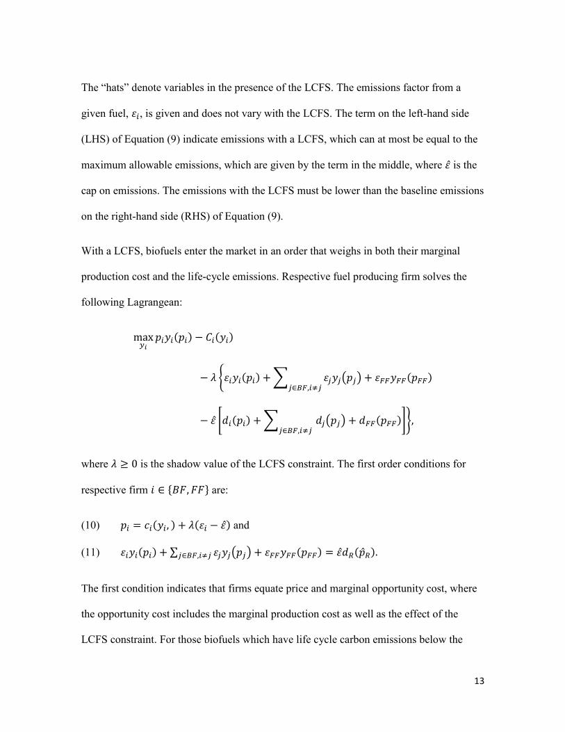
The “hats” denote variables in the presence of the LCFS. The emissions factor from a

given fuel, 휀𝑖, is given and does not vary with the LCFS. The term on the left-hand side

(LHS) of Equation (9) indicate emissions with a LCFS, which can at most be equal to the

maximum allowable emissions, which are given by the term in the middle, where 휀̂ is the

cap on emissions. The emissions with the LCFS must be lower than the baseline emissions

on the right-hand side (RHS) of Equation (9).

With a LCFS, biofuels enter the market in an order that weighs in both their marginal

production cost and the life-cycle emissions. Respective fuel producing firm solves the

following Lagrangean:

max𝑦𝑖

𝑝𝑖𝑦𝑖(𝑝𝑖) − 𝐶𝑖(𝑦𝑖)

− 𝜆 {휀𝑖𝑦𝑖(𝑝𝑖) + ∑ 휀𝑗𝑦𝑗(𝑝𝑗)𝑗∈𝐵𝐹,𝑖≠𝑗

+ 휀𝐹𝐹𝑦𝐹𝐹(𝑝𝐹𝐹)

− 휀̂ [𝑑𝑖(𝑝𝑖) + ∑ 𝑑𝑗(𝑝𝑗)𝑗∈𝐵𝐹,𝑖≠𝑗

+ 𝑑𝐹𝐹(𝑝𝐹𝐹)]},

where 𝜆 ≥ 0 is the shadow value of the LCFS constraint. The first order conditions for

respective firm 𝑖 ∈ {𝐵𝐹, 𝐹𝐹} are:

(10) 𝑝𝑖 = 𝑐𝑖(𝑦𝑖, ) + 𝜆(휀𝑖 − 휀̂) and

(11) 휀𝑖𝑦𝑖(𝑝𝑖) + ∑ 휀𝑗𝑦𝑗(𝑝𝑗)𝑗∈𝐵𝐹,𝑖≠𝑗 + 휀𝐹𝐹𝑦𝐹𝐹(𝑝𝐹𝐹) = 휀̂𝑑𝑅(�̂�𝑅).

The first condition indicates that firms equate price and marginal opportunity cost, where

the opportunity cost includes the marginal production cost as well as the effect of the

LCFS constraint. For those biofuels which have life cycle carbon emissions below the

14

level of the LCFS (휀̂), the second term on the RHS of Equation (10) is negative. The

LCFS thus constitutes a subsidy to these fuels, which can be produced in greater quantities

than in the absence of the LCFS. The subsidy is higher for fuels with lower life cycle

carbon emissions. For those fuels with greater life-cycle emissions than the LCFS baseline

the second term is positive. This acts as a tax on these fuels. The LCFS thus affects the

fuel mix. The second condition, Equation (11), is the complementary slackness condition.

Equations (10) and (11) characterize supply while demand is given by 𝑑𝑅(𝑝𝑅) = �̂�𝑅.

Unlike in the case of a biofuel mandate, with a LCFS all fuels face the same average fuel

price. Substituting Equation (10) into the average fuel price (2) yields the equilibrium

price under LCFS:

(12) �̂�𝑅 = ∑ �̂�𝑖[𝑐𝑖(𝑦𝑖) + 𝜆(휀𝑖 − 휀̂)]𝑖∈𝐵𝐹 + (1 − �̂�)[𝑐𝐹𝐹(𝑦𝐹𝐹) + 𝜆(휀𝐹𝐹 − 휀̂)].

In the present formulation the LCFS, too, is a cost efficient policy instrument since it

equates the marginal opportunity cost for all fuels.

A simple illustration of the LCFS assuming zero-emission biofuels is shown in Figure 2.

In reality, zero-emission biofuels do not exist. Baseline emissions, 휀𝑑𝑅(𝑝𝑅) in Figure 2

are equal to total fuel demand, which does not shift with the LCFS. The target emissions,

however, are lower, at 휀̂𝑑𝑅(𝑝𝑅). The thick black line in Figure 2 shows the maximum

possible consumption of fossil fuels if the LCFS is to be reached at the prevailing fossil

fuel price, 𝑝𝐹𝐹. In terms of the figure, zero life-cycle emission biofuels will have to be

used to fill the gap between possible fossil fuels consumption and fuel demand. The curve

15

𝑦𝐵𝐹(�̂�𝐵𝐹) gives the supply of zero emission biofuels. These are assumed to have a higher

marginal production cost than fossil fuels.

2.5 The system of policy instruments

Examining the biofuel mandate and the LCFS together yields the first proposition:

Proposition 1. Either the biofuel mandate or the LCFS is redundant.

Proof: The two policy instruments imposed by EU legislation can be set up as a Lagrange

maximization problem:

max𝑦𝑖,𝑦𝐹𝐹

𝑝𝑖𝑦𝑖(𝑝𝑖) − 𝐶𝑖(𝑦𝑖) − 𝛿 [�̅�𝑑𝑅(𝑝𝑅) − ∑ 𝑦𝑖(𝑝𝑖)

𝑖∈𝐵𝐹

]

− 𝜆 [ ∑ 휀𝑖𝑦𝑖(𝑝𝑖)

𝑖∈𝐵𝐹

+ 휀𝐹𝐹𝑦𝐹𝐹(𝑝𝐹𝐹) − 휀̂𝑑𝑅(𝑝𝑅)]

With two restrictions (policy instruments that force the consumption of biofuels with the

corresponding complementary slackness conditions), we have a Kuhn-Tucker –type of

problem where only one restriction at a time can bind. ■

3 Results and discussion

In this section we use the models described in Sections 2.2 to 2.4 to analyse double

counting in the presence of a biofuel mandate and a LCFS, respectively. Thereafter we

consider the impact of a particular type of technological change, namely one that lowers

the marginal production cost of biofuels. We end by examining the interplay between

three national-level policy instruments and the biofuel mandate and LCFS.

16

3.1 A biofuel mandate with double counting

‘Double counting’ was described in the introduction. We decompose the total supply of

biofuels into two types, namely to single-counted ones (SC) and to double counted ones

(DC). This yields the following biofuel mandate instead of (3):

(13) �̅� =∑ �̅�𝑖(�̅�𝑖)𝑖∈𝑆𝐶 +2 ∑ �̅�𝑗(�̅�𝑗)𝑗∈𝐷𝐶

𝑑𝑅(�̅�𝑅).

Straight out counting some biofuels twice would increase the reported share of biofuels

out of the total fuel consumption. The biofuel mandate remains constant with double

counting, however. Thus, the actual amount of biofuels on the market will have to fall so

that the reported amount of biofuels does not exceed the mandate. Setting up the Lagrange

function corresponding to Equation (13) yields:

max𝑦𝑖,𝑦𝐹𝐹

𝑝𝑖𝑦𝑖(𝑝𝑖) − 𝐶𝑖(𝑦𝑖, 𝑤𝑖) − 𝛿𝐷𝐶 {�̅� [ ∑ 𝑦𝑖

𝑘∈𝐵𝐹

+ 𝑦𝐹𝐹] − ∑ 𝑦𝑖

𝑖∈𝑆𝐶

− 2 ∑ 𝑦𝑗

𝑗∈𝐷𝐶

}.

𝛿𝐷𝐶 ≥ 0 is the shadow value of the biofuel mandate in the presence of double counting. It

is directly apparent that the constraint from the biofuel mandate with double counting is

less stringent than the constraint without double counting. This implies that the shadow

price of the constraint tends to fall, so that 𝛿𝐷𝐶 ≤ 𝛿. The first order condition for the

doubly counted biofuels is

(14) 𝑝𝑖 = 𝑐𝑖(𝑦𝑖) + 𝛿𝐷𝐶(�̅� − 2)

17

The remaining first order conditions are still given by Equations (5) - (7). The prices of all

biofuels are equalized with one another. If this was not the case, demand for the more

expensive biofuel would fall until prices were equalized. Double counting influences the

price of biofuels:

Proposition 2. Double counting lowers the price of biofuels.

Proof: We write the actual share of biofuels with double counting as

�̅�𝐷𝐶 =𝑑𝐵𝐹

𝑆𝐶 (�̅�𝐵𝐹)+𝑑𝐵𝐹𝐷𝐶(�̅�𝐵𝐹)

𝑑𝑅(�̅�𝑅)< �̅�. If the price of biofuels remained constant or increased,

supply of biofuels would exceed the biofuel mandate. This can also be seen from the

Lagrangean. ■

The falling price of biofuels has implications to the supply of biofuels:

Proposition 3. Double counting increases the production of the doubly counted biofuels

given that the shadow price on the biofuel mandate constraint does not fall ‘too low’

(𝜹𝑫𝑪 >�̅�−𝟏

�̅�−𝟐𝜹).

Proof: We examine the implications of the falling price of biofuels, that is, 𝑝𝐵𝐹 > 𝑝𝐵𝐹𝐷𝐶 as

given in Equations (5) and (14). Moving terms around yields

(15) 𝑐𝐵𝐹𝐷𝐶 − 𝑐𝐵𝐹 < 𝛿(�̅� − 1) − 𝛿𝐷𝐶(�̅� − 2).

We have assumed marginal costs to increase in increased production, which implies that

the production of the doubly counted biofuels increases if 𝑐𝐵𝐹𝐷𝐶 > 𝑐𝐵𝐹. The LHS of

Equation (15) is then positive. The RHS then also must be positive, which implies

18

𝛿𝐷𝐶 >�̅�−𝟏

�̅�−𝟐 𝛿. At �̅� = 0 this simplifies to 𝛿𝐷𝐶 >

1

2𝛿, that is, if the shadow value of the

biofuel mandate falls by more than half, then the production of the doubly counted

biofuels falls as compared to no double counting. At the other extreme, �̅� = 1, it

simplifies to 𝛿𝐷𝐶 > 0, which is always true. Between these extreme values, �̅�−𝟏

�̅�−𝟐 is a

falling concave function. It is depicted in Figure 3. ■

The corollary of Propositions 2 and 3 is that the production of the singly counted biofuels

falls. Proposition 2 implies that 𝑝𝐵𝐹𝑆𝐶 < 𝑝𝐵𝐹. Substituting from Equation (5) yields after

simplification 𝑐𝐵𝐹𝑆𝐶 − 𝑐𝐵𝐹 < (𝛿 − 𝛿𝐷𝐶)(�̅� − 1), where the RHS is always negative.

The marginal production cost of the doubly counted biofuels will exceed the marginal

production cost of the single-counted biofuels, which can be seen by equating their prices,

𝑝𝐵𝐹𝑆𝐶 = 𝑝𝐵𝐹

𝐷𝐶, using Equations (5) and (14) and simplifying, which yield 𝑐𝐵𝐹𝐷𝐶 − 𝑐𝐵𝐹

𝑆𝐶 = 𝛿𝐷𝐶.

The difference in the marginal production costs therefore equals the shadow price of the

biofuel mandate. Double counting therefore makes the biofuel mandate non-cost-efficient.

The average fuel price with double counting is �̅�𝑅𝐷𝐶 = ∑ �̅�𝑖

𝐷𝐶�̅�𝐵𝐹𝐷𝐶

𝑖=𝐵𝐹 + (1 − �̅�𝐷𝐶)�̅�𝐹𝐹𝐷𝐶.

Since �̅�𝐵𝐹𝐷𝐶 ≤ �̅�𝐵𝐹 and �̅�𝐹𝐹

𝐷𝐶 > �̅�𝐹𝐹, the total effect of double counting on the average price

of fuel is ambiguous. We examine under what circumstances double counting may raise

the average price of fuel. Substituting yields the following:

(16) ∑ [�̅�𝑖𝐷𝐶�̅�𝐵𝐹

𝐷𝐶 − �̅�𝑖�̅�𝐵𝐹]𝑖=𝑆𝐶 + ∑ [�̅�𝑗𝐷𝐶�̅�𝐵𝐹

𝐷𝐶 − �̅�𝑗�̅�𝐵𝐹]𝑗=𝐷𝐶 + (1 − �̅�𝐷𝐶)�̅�𝐹𝐹𝐷𝐶 −

(1 − �̅�)�̅�𝐹𝐹 > 0.

19

The terms in the first and the second brackets of Equation (16) are negative because of the

falling price and share of biofuels. The difference in the two last terms, (1 − �̅�𝐷𝐶)�̅�𝐹𝐹𝐷𝐶 and

(1 − �̅�)�̅�𝐹𝐹 is positive, however. The total effect on the average price of fuels then

depends on whether the negative effect from the biofuels’ market share and price, or the

positive effect from the fossil fuels market share and price overweigh in Equation (16).

Double counting provides certain extra support for the producers of the doubly counted

biofuels. The impact of double counting is however mitigated by its impact on the biofuel

mandate constraint, which becomes less binding. In fact, double counting functions as a

type of subsidy to the consumption of fossil fuels since it lowers the required amount of

biofuels on the market and therefore allows fossil fuels’ price and actual market share to

increase.

3.2 The low carbon fuel standard and double counting

Double counting makes the biofuel mandate easier to fill. Then, even if the biofuel

mandate is the binding policy instrument without double counting, it may be that double

counting leads to a switch in which of the two policy instruments that binds.

Double counting is a policy connected to the biofuel mandate, not to the LCFS.

Accounting for the consumption of certain biofuels twice in the statistics delivered to the

EU does not change the life-cycle emissions from a given fuel mix. Considering that a

binding LCFS, as it is, increases biofuel consumption beyond the level required by the

biofuel mandate, double counting some biofuels only increases the ‘over filling’ of the

biofuel quota.

20

3.3 The impact of technical change

We study how technical change affects and are affected by the biofuel mandate and the

LCFS with and without double counting. Technical change is possible in several parts of

the system: 1. Technical change could increase the amount of biofuel produced per unit of

feedstock, 2. Technical change can change the feedstock used to produce a biofuel, and 3.

Technical change could lower the production cost of the feedstock. Furthermore, if

technical change influences the production technology used to produce the feedstock,

technical change can lower the life-cycle carbon emissions from a fuel without affecting

the marginal production costs.6

We examine here only the case where technical change affects the marginal production

cost of a biofuel, and where technical change is a function of past production, that is, we

assume some kind of experience curves (Neij, 2008; Bergek and Jacobsson, 2010).

Production of biofuel 𝑖 is then given by 𝑦𝑖(𝑝𝐵𝐹, 𝑝𝐹𝐹; 𝐴𝑖, 𝑌𝑡), where 𝑌𝑡 denotes the stock of

past production, 𝐴𝑖 ≥ 0 is a parameter measuring how past production affects present

production and 𝜕𝑦𝑖

𝜕𝐴𝑖𝑌𝑡> 0. If 𝐴𝑖 = 0, there is no technological progress based on the stock

of past production. We assume that the cost of the feedstock remains approximately

constant, and that there is no technical progress in the feedstock production.

6 There is nothing automatic about technological change, nor do we have a very good understanding of the

process. For example, Tyner (1980, p. 961) wrote: “… By the mid-1980s, most authorities believe that

cellulose conversion technologies will be commercially available to produce ethanol from crop residues,

forage crops, wood, or municipal solid waste…”

21

In order to determine the equilibrium price of biofuels after technical change, we use

Equation (4). The RHS of (4) is unaffected by technical change since technical change

does not shift the demand function and the biofuel mandate is not automatically adjusted

to lower production costs. The LHS changes, however since the supply of biofuel 𝑖

increases given the producer price, �̅�𝐵𝐹. Since the biofuel mandate is unchanged, the

producer price of biofuels falls. This fall in the price lowers the production of the other

biofuels 𝑗 ∈ 𝐵𝐹, 𝑖 ≠ 𝑗. The relative shares of biofuels change so that the share of biofuel 𝑖,

�̅�𝑖 increases and the sum of shares of the other biofuels, ∑ �̅�𝑗𝑗∈𝐵𝐹,𝑖≠𝑗 falls. In equilibrium,

demand adjusts to the lower average fuel price. Double counting does not change this

analysis. It affects the pace of experience-related technical development, however:

Proposition 4. Double counting with a biofuel mandate increases technical development

in the doubly counted biofuels if 𝜹𝑫𝑪 >�̅�−𝟏

�̅�−𝟐𝜹, but reduces it in the single-counted

biofuels if technical development is a function of past production.

Proof: As was shown in Proposition 3, double counting increases the production of the

double counted biofuels given that 𝛿𝐷𝐶 >�̅�−1

�̅�−2𝛿. Greater past production is assumed to

increase the pace of technical development and therefore double counting increases the

technical progress in the doubly counted biofuels. After Proposition 3 we showed that the

production of the single-counted biofuels falls. Therefore, technical progress in these

biofuels also slows down. ■

22

As was noted in the introduction, the EU introduced double counting in order to promote

technical development of the doubly counted biofuels. We therefore conclude that double

counting with a biofuel mandate as a policy instrument works approximately as planned.

With the LCFS, technical development does not change the demand for fuel in the middle

part of Equation (9). It does, however, increase supply given the producer price, �̅�𝐵𝐹. We

formulate the main impact of technical change under a LCFS in the following proposition:

Proposition 5. Technical change in the below LCFS emission biofuels (𝜺𝒊 < �̂�) it lowers

the cost of meeting the LCFS. Technical change in an above LCFS emissions fuel (𝜺𝒊 > �̂�)

raises the cost of meeting the LCFS.

Proof: We prove Proposition 5 by examining Equation (11) together with (10). If the

biofuel experiencing technical change is a low life-cycle emission one, the last term on the

RHS of (10) is negative. Increasing the production of this type of biofuel in (11) then

lowers the average emissions thereby making the LCFS constraint easier to fulfil. This

lowers the shadow price, which makes the LCFS cheaper to meet. Similarly, if the fuel

experiencing technical development is a high life-cycle emission one, the last term on the

RHS of (10) is positive. In terms of (11), increased production would raise the average

emissions. The LCFS hinders this, however, but since the marginal production cost of the

more polluting fuels falls, the shadow price of the LCFS constraint must increase to keep

up the supply of low-emission biofuels. ■

Proposition 5 has consequences for technological change. If the shadow price falls, and

the subsidy given to low-emission biofuels therefore falls, production falls. Technical

23

change then reduces future technical change in these fuels. On the other hand, an

increasing shadow price creates incentives to increased production. The LCFS both

hinders increased production of the high-emission fuels and raises the implicit subsidy to

the low-emission biofuels, thereby increasing production. This in turn may increase

technical development of the low-emission biofuels.

3.4 National-level policy instruments: exemption from fuel duty, feed-in tariffs and

tradable biofuel certificates

In this section we shortly describe how double counting works in the presence of national-

level policy instruments. We examine three policy instruments that EU member states

have used, or could use to promote the production and consumption of biofuels:

exemptions from fuel duty or CO2 taxation (at least Germany, Sweden), feed-in tariffs

(used to promote renewable electricity production in for example Germany) and tradable

biofuel certificates (Sweden has a comparable system for renewable electricity

production).

3.4.1 Fuel and/or CO2 tax exemptions

de Gorter and Just (2009) analyse fuel duties together with a biofuel mandate. A fuel

duty, 𝜏𝑖, drives a wedge between the producer and consumer prices of fuels. Denoting the

producer price by �̅�𝑖 (�̂�𝑖 when analysing a LCFS), the consumer price in the presence of a

biofuel mandate (LCFS) and a fuel duty becomes �̅�𝑖 = �̅�𝑖 + 𝜏𝑖 (�̂�𝑖 = �̂�𝑖 + 𝜏𝑖), 𝑖 ∈

{𝐵𝐹, 𝐹𝐹}. Applying an equal fuel duty to all fuels yields the average fuel price of �̅�𝑅 =

24

�̅��̅�𝐵𝐹 + (1 − �̅�)�̅�𝐹𝐹, where �̅� is defined in Equation (3) (�̂�𝑅 = �̂��̂�𝐵𝐹 + (1 − �̂�)�̂�𝐹𝐹).

This is higher than in the absence of a fuel duty.

Giving all biofuels an equal exemption from fuel duty lowers their consumer price to �̅�𝐵𝐹

(�̂�𝐵𝐹). The average fuel price becomes �̅�𝑅𝑇𝐸 = �̅��̅�𝐵𝐹 + (1 − �̅�)�̅�𝐹𝐹 (�̂�𝑅

𝑇𝐸 = �̂��̂�𝐵𝐹 +

(1 − �̂�)�̂�𝐹𝐹) where the superscript TE denotes ‘tax exemption’. With a biofuel mandate,

the consumption of biofuels is still dictated by the mandate so biofuel consumption is not

affected. The average fuel price however falls. This boosts demand for all fuel. As is

shown by de Gorter and Just, a combined biofuel mandate – fuel tax exemption thus

constitutes a subsidy to all fuel consumption.

With LCFS increased demand for fuel raises absolute emissions. The LCFS allows for

increased emissions, however, since in the baseline equation, the emissions factor is fixed

but not consumption. Even in the presence of a LCFS, a fuel tax exemption therefore

constitutes a subsidy to all fuel consumption.

Double counting with a fuel tax exemption in the presence of a biofuel mandate serves to

lower the actual consumption of biofuels and therefore their price. The results in

Proposition 3 still hold. The LCFS is not affected by double counting.

3.4.2 Feed-in tariffs

To keep the analysis simple, we analyse a fixed-rate feed-in tariff paid to all biofuels. We

furthermore assume that the feed-in tariff is paid for from general tax revenue and not as a

25

surcharge on fuel prices.7 The consumer prices of fuels remain as in the basic model,

denoted by 𝑞𝑖, 𝑖 ∈ {𝐵𝐹, 𝐹𝐹}. The producer price of fossil fuels is given by 𝑝𝐹𝐹 = 𝑞𝐹𝐹. The

producer price of biofuels, however, is affected by the feed-in tariff and becomes 𝑝𝐵𝐹𝐹𝑇 =

𝑝𝐹𝐹 + 𝑓, where 𝑓 is the feed-in tariff and the superscript FT denotes the ‘feed-in tariff’.

Thus, biofuels are produced up to a point where the marginal production cost equals the

producer price: 𝑐[𝑑𝐵𝐹(𝑝𝐵𝐹)] = 𝑝𝐹𝐹 + 𝑓.

The price implied by the feed-in tariff, 𝑝𝐵𝐹𝐹𝑇, may exceed or fall short of the equilibrium

price to fill the biofuel mandate (LCFS), �̅�𝐵𝐹 (�̂�𝐵𝐹). If the feed-in tariff exceeds the

equilibrium price, more biofuels will be produced than the mandate (LCFS) dictates. If it

falls short, the price will rise to the level required by the biofuel mandate (LCFS). Thus,

even here we have a Kuhn-Tucker type of condition where only one policy instrument at a

time binds.

With a LCFS it is further possible that the production of the more polluting biofuels rise

with the introduction of the feed-in tariff compared to a LCFS only. The production of

biofuels is first determined by the condition equating the marginal production cost with

the producer price. If emissions from this production level are lower than the emissions

required by the LCFS, the LCFS is redundant. If, however, emissions exceed the

emissions allowed by the LCFS, the market works in effect like described in Section 2.4.

7 The case of feed-in tariffs financed from a surcharge on fuel prices is more complicated than the present

one but does not yield much more information. The complications are due to the equilibrium effects on

the fuel market that arise from the surcharge.

26

We assume that doubly counted biofuels obtain double feed-in tariff. They will

consequently be produced up to a point where 𝑐[𝑑𝐵𝐹𝐷𝐶(𝑝𝐵𝐹

𝐷𝐶)] = 𝑝𝐹𝐹 + 2𝑓. If the producer

price of the doubly counted biofuels with a double feed-in tariff exceeds the producer

price of biofuels with only a biofuel mandate ( �̅�𝐹𝐹 + 2𝑓 > �̅�𝐵𝐹), the production of the

doubly counted biofuels rises beyond their production level with only a biofuel mandate,

and vice versa if the price falls short of the equilibrium price for a biofuel mandate only.

It is also possible that 𝑝𝐹𝐹 + 𝑓 < �̅�𝐵𝐹 < 𝑝𝐹𝐹 + 2𝑓, that is, that the producer price which is

required to fulfil the biofuel mandate lies between the producer prices of the single-

counted and the doubly counted biofuels with a feed-in tariff. In this case the price of the

single-counted biofuels depends on whether the production of the doubly counted

biofuels, when counted twice towards the quota, is sufficiently high for the biofuel

mandate to be satisfied. If not, the producer price of the single-counted biofuels will have

to rise until the biofuel mandate is satisfied. This does not affect the producer price of the

doubly counted biofuels.

Since the doubly counted biofuels, which get a double feed-in tariff, are mainly low life-

cycle emission biofuels it may become more probable that the combined feed-in tariff –

LCFS are in line with one another. Nevertheless, it is unlikely that the feed-in tariff can be

determined so as to yield exactly the prices needed to reach the LCFS.

3.4.3 Tradable biofuel certificates

A biofuel certificate is a proof of production and consumption of one unit of biofuels. The

certificates are given to the producers of biofuels and follow each unit of biofuels to their

27

end consumers.8 The certificate price equals the shadow price of the biofuel mandate. If

trade in the certificates is allowed between fuel consumers, a consumer who cannot

consume the required amount of biofuels can buy a certificate from another consumer who

over-consumes biofuels instead. This equalizes the certificate prices across all biofuels

and also the prices of all biofuels with one another.

With biofuel certificates, the doubly counted biofuels could get two certificates. Equation

(13) still holds, however, so the actual amount of biofuels consumed falls when double

counting is allowed. Propositions 2 and 3 still hold.

With a LCFS, we assume that all (eligible) biofuels that enter the market get a biofuel

certificate. The certificate price rises to a level needed to fill the LCFS, and equals the

shadow price of the LCFS constraint. Since the certificate price is uniform for all biofuels

regardless of emissions, a problem similar to that with the feed-in tariffs may arise.

Double counting, and the ensuing double allocation of certificates to low life-cycle

emission biofuels may then mitigate the problem by increasing the supply of the low-

emission biofuels more than the supply of more polluting biofuels. Unlike in the case of

the feed-in tariff, the biofuel certificate price nevertheless adjusts to a level as close to the

optimum as possible.

8 In practice it may be impractical to demand certificates from consumers of fuel. Then it would be the fuel

distributors who would have to be able to present a certain amount of certificates relative to their total

fuel sales.

28

The LCFS combined with biofuel certificates and double counting may however also lead

to considerable price instability. The certificate price is determined by the ‘marginal’

biofuel; that is the highest cost biofuel entering the market under the LCFS. If this is a

doubly counted biofuel, it obtains two certificates, and the certificate price is half of what

the marginal biofuel obtains. Depending on the certificate price, the production of the

single-counted biofuels further down the ‘merit order’ adjusts, and may actually fall

considerably. If their production falls sufficiently so that the LCFS is not reached, the

certificate price will have to rise to increase the production of these biofuels. This may

create price instability at least in the short run. If the marginal biofuel is a single-counted

one, this problem does not arise, however. It is also worth noting that the problem does

not arise with feed-in tariffs whose level is administratively fixed.

4 Conclusions and policy implications

The results in this paper are unsurprising, yet important. The EU has created a system of

policy instruments that, by regulating the consumption of biofuels from several different

directions, includes (at least) one binding and one redundant policy instrument. Since

compliance with both the biofuel mandate and the low carbon fuel standard have to be

ensured, both create costs, however. This is a thoroughgoing theme in EU legislation in

the climate- and energy areas, other examples including the interaction between the

emissions trading system (ETS) on one hand, and the renewable electricity targets

included in the RED on the other, and the interaction between the ETS and energy

efficiency targets. It is also a problem at the implementation stage at the Member State

29

level, too, which the example of the interplay between the biofuel mandate, the LCFS and

the feed-in tariffs demonstrates.

Double counting of some biofuels is a policy instrument that is unique for the transport

sector. While it fulfils its purpose if the biofuel mandate is the binding policy instrument,

by increasing the production of the doubly counted biofuels and therefore raising the pace

of experience-based technological progress, it does this at the expense of cost-efficiency.

Thus, the marginal production costs of the single- and double counted biofuels will not be

equalized. It should be reconsidered whether this is a desirable way of promoting the

doubly counted biofuels and spurring hoped-for technological progress.

If the LCFS is the binding policy instrument, double counting does not matter, but still

creates compliance and monitoring costs. Unlike the biofuel mandate, the LCFS

subsidizes most those biofuels that have the lowest life cycle emissions. Therefore it gives

most support to the most meriting biofuels in a cost efficient manner.

The implication of these results is a need to see over the EU’s policy packages. Reducing

emissions of greenhouse gases and revamping the energy and transport systems is costly

as such; creating an overtly complex and partly redundant system of policies only raises

that cost. The results also highlight the importance of choosing sensible Member State

level policies to implement EU legislation. Otherwise policy risks including redundant

policy instruments, becoming non-cost-efficient, or creating unwanted side effects, like

subsidising fossil fuels instead of biofuels, as the example of fuel and/or CO2 tax

exemptions in conjunction with a biofuel mandate shows. If the EU policy to start with

30

has some or all of these features, ways to remedy them as far as possible at the Member

State level should be found.

Acknowledgements

An earlier version of the paper was presented at the First National Conference in

Transport Research, Stockholm, 18-19 October 2012.

References

Andress, D., Nguyen, T. D. & Das, S., 2009. Low-carbon fuel standard - Status and

analytic issues. Energy Policy, 38, 580-591.

Bandyopadhyay, S., Bhaumik, S. & Wall, H. J., 2013. Biofuel subsidies and international

trade. Economic & Politics, 25(2), 181-199.

Baral, A., 2009. Summary report on low carbon fuel-related standards, International

Council on Clean Transportation.

Bergek, A. & Jacobsson, S., 2010. Are tradable green certificates a cost-efficient policy

driving technical change or a rent-generating machine? Lessons from Sweden 2003-2008.

Energy Policy, 38, 1255-1271.

Chi, J., Lapan, H., Moschini, G. & Cooper, J., 2011. Welfare impacts of alternative

biofuel and energy policies. American Journal of Agricultural Economics, 93(5), 1235-

1256.

31

Crago, C. L. & Khanna, M., 2009. Welfare effects of biofuels trade policy in the presence

of environmental externalities, Available at SSRN: http://ssrn.com/abstract=1367101.

de Gorter, H. & Just, D. R., 2009. The economics of a blend mandate for biofuels.

American Journal of Agricultural Economics, 91(3), 738-750.

Eggert, H. & Greaker, M., 2012. Trade policies for biofuels. The Journal of Environment

& Development, 21(2), 281-306.

Greaker, M., Hoel, M. & Rosendahl, K. E., 2012. Does a renewable fuel standard for

biofuels reduce climate costs?, CESifo Working Paper No 4030.

Holland, S. P., Hughes, J. E., Knittel, C. R. & Parker, N. C., 2011. Some inconvenient

truths about climate change policy: The distributional impacts of transportation policies.

NBER Working Paper Series, 17386.

Holland, S. P., Knittel, C. R. & Hughes, J. E., 2008. Greenhouse gas reductions under low

carbon fuel standards?, University of California Davis.

Jussila Hammes, J., 2014. Kvotplikt för biodrivmedel - högsta vinsten till

specialintressen?. Ekonomisk debatt, 2, 42-51.

Le Roy, D. G., Elobeid, A. E. & Klein, K. K., 2011. The impact of trade barriers on

mandated biofuel consumption in Canada. Canadian Journal of Agricultural Economics,

59(4), 457-474.

32

Neij, L., 2008. Cost development of future technologies for power generation - A study

based on experience curves and complementary bottom-up assessments. Energy Policy,

36, 2200-2211.

Swedish Energy Agency, 2009. Kvotpliktsystem för biodrivmedel. Energimyndighetens

förslag till utformning. Eskilstuna: Swedish Energy Agency.

Tyner, W. E., 1980. Our Energy Transition: The Next Twenty Years. American Journal of

Agricultural Economics, 62(5), 957-964.

Yeh, S. & Sperling, D., 2010. Low carbon fuel standards: Implementation scenarios and

challenges. Energy Policy, 38, 6955-6965.

33

Figures

Figure 1. Share of renewable energy in transport, selected EU countries and the average

for 28 EU countries. Source: Eurostat.

0,0

2,0

4,0

6,0

8,0

10,0

12,0

14,0

2004 2005 2006 2007 2008 2009 2010 2011 2012

EU (28 countries)

Germany

France

Italy

Sweden

United Kingdom

34

Figure 2. The LCFS. Fuel demand is given by the curve 𝒅𝑹(𝒑𝑹) = 𝜺𝒅𝑹(𝒑𝑹), while

�̂�𝒅𝑹(𝒑𝑹) gives the LCFS. The supply of fossil fuels is given by 𝒚𝑭𝑭(𝒑𝑭𝑭) and is, for

simplicity, assumed to be completely elastic. The LCFS limits the consumption of fossil

fuels to a maximum amount of 𝒀𝑭𝑭𝑳𝑪𝑭𝑺 (the thick vertical line). In order to meet demand,

zero-emission biofuels will have to be consumed (if no zero-emission biofuels are

available, fossil fuel consumption will have to fall further). For ease of exposition, the

intercept of the biofuel supply curve 𝒚𝑩𝑭(𝒑𝑩𝑭) is arbitrarily set to coincide with the price

of fossil fuels. The LCFS thus forces biofuels into the market and yields the fuel supply

curve denoted by 𝒚𝑹(𝒑𝑹). At the equilibrium price 𝒑𝑹 the quantity of biofuels consumed

is 𝒀𝑩𝑭𝑳𝑪𝑭𝑺.

𝑌𝐵𝐹𝐿𝐶𝐹𝑆

𝑦𝐹𝐹(𝑝𝐹𝐹)

휀𝑑𝑅(𝑝𝑅) 휀̂𝑑𝑅(𝑝𝑅) 𝑦𝐵𝐹(𝑝𝐵𝐹)

𝑦𝑅(�̂�𝑅)

𝑌𝑖

𝑝𝑖

𝑌𝐹𝐹𝐿𝐶𝐹𝑆

�̂�𝑅

35

Figure 3. The minimum value frontier for 𝜹𝑫𝑪 >�̅�−𝟏

�̅�−𝟐𝜹.

0

0,1

0,2

0,3

0,4

0,5

0,6

0

0,0

5

0,1

0,1

5

0,2

0,2

5

0,3

0,3

5

0,4

0,4

5

0,5

0,5

5

0,6

0,6

5

0,7

0,7

5

0,8

0,8

5

0,9

0,9

5 1

δ^DC>

ω

(ω-1)/(ω-2)