a bioeconomic model for determining the optimal response...

A bioeconomic model for determining the optimal

response to a new weed incursion in Australian cropping

systems

Rohan T. Jayasuriya and Randall E. Jones

CRC for Australian Weed Management and NSW Department of Primary Industries, Orange Agricultural Institute, Forest Road, Orange NSW 28001

Contributed paper presented to the 52nd Annual Conference of the Australian Agricultural and

Resource Economics Society, Canberra, 5-8 February 2008

Abstract Invasions by non-indigenous plant species pose serious economic threats to Australian agricultural industries. When an invasion is discovered a decision has to be made as to whether to attempt to eradicate it, contain it or do nothing. These decisions should be based on long term benefits and costs. This paper describes a bioeconomic simulation framework with a mathematical model representing weed spread linked to a dynamic programming model to provide a means of determining the economically optimal weed management strategies over time. The modelling framework is used to evaluate case study invasive weed control problems in the Australian grains industry. Keywords: weeds, incursion, bioeconomic model Contact details: Rohan T. Jayasuriya, NSW Department of Primary Industries, Orange Agricultural Institute, Forest Road, Orange NSW 2800 Tel: +61 2 6391 3826, E-mail: [email protected]

1 The views expressed in this paper are those of the authors, rather than those of NSW Department of Primary Industries or the NSW Government.

A bioeconomic model for determining the optimal response to a new weed incursion in Australian cropping systems

_______________________________________________________________________________________

52 nd

Annual AARES Conference, Canberra, 5-8 February 2008 of 25

1. Introduction Invasions by non-indigenous plant species pose serious economic threats to Australian agricultural industries. Effective quarantine strategies are the key to managing the risk of exotic invasive species. However, there is always a risk of new invasions due to international trade and travel by individuals. Moreover, there is also the threat of previously unidentified “sleeper weeds” emerging. Consequently, it is important to have well developed strategies for dealing with new incursions as they occur, rather than relying on a reactive approach to managing incursions. The current cost of weeds in Australian cropping systems is around $1.5 billion per annum (Sinden et al., 2004) which represents 15% of the 2001-02 gross value of the Australian grains industry. This is the current cost of weed infestations only and ignores the potential future costs that may occur from new weed incursions. In general, early action on invasive plants can give significantly greater economic results than waiting for the weed problem to develop into one of significance before taking action. Once an infestation is well established the policy and management options may become limited, and the economic returns from strategies such as eradication may then be negative. Consequently, an efficient allocation of capital and scarce resources may be to deal with new weed incursions in preference to existing large scale infestations. The issue of weed incursion management has been considered for natural ecosystems, where there is a well understood role of government, but in cropping systems this issue has not been well discussed. In particular the roles of government and private landholders need to be considered, given that there are potential private as well as public benefits and costs associated with a new weed incursion. When a new invader is identified rapid response is critical, particularly if the invasive plant has the ability to spread rapidly. A decision on whether to eradicate or contain the infestation, or leave it to landholders to manage needs to be made early. This decision will be based upon the benefits and costs over time associated with each option. Weed eradication can be particularly costly and usually involves long-term commitments of public funds, whereas leaving management to landholders can result in an increase in the private costs to an industry as an invasive species spreads over time. At present there is a lack of a decision making process to determine the economically optimal strategies for dealing with new weed incursions in cropping systems. Therefore, decision support models have a role as tools for weed management. Currently available weed management models range in sophistication from herbicide selection models based on efficacy to threshold based bioeconomic models, featuring cost/benefit analysis (Martin et al., 1998). Ascertaining more biological information concerning weed emergence, competition, seed production, mortality, and composition of weed populations is critical in bioeconomic weed management models. Other weaknesses of the models and the ability to use them that need to be dealt with are estimating weed-free crop yields, characterizing weed spatial variability, and maintaining and expanding databases on weed control efficacy of herbicide-susceptible and resistant weed species (Schweizer et al., 1998). The first section of this paper presents a flexible modelling approach that incorporates the key processes that determine the spatial population dynamics of an invading plant species in a large area cropping system. This spatially explicit spread model is then linked to a dynamic programming model, which determines the economically optimal weed management strategies for


_______________________________________________________________________________________

52 nd


various infestation level states. A bioeconomic modelling framework such as described here can have considerable value to government and the Australian grains industries to assist the development of more effective alien plant management strategies. In this paper, the modelling framework is used to evaluate case study invasive weed control problems in the Australian grains industry.

2. The bioeconomic framework

An important motivation for a bioeconomic modelling approach is the expectation to achieve economic and environmental gains by using flexible weed management plans in which weed control is varied each year based on observed conditions instead of fixed plans. Typically, weed scientists and modellers use mathematical bioeconomic models to link observed conditions such as weed seedling densities to annual weed management recommendations (Kwon et al., 1995). The decision framework uses experimental results, field data, and expert opinion to define biological relationships between weeds and crops, which are then incorporated into an optimising economic model. As discussed by Kwon et al. (1995), most U.S. bioeconomic weed management studies have involved corn, soybeans, cotton, potatoes or sugar beets while similar work in wheat has been done outside the U.S. Most economic weed management studies have focused on a single weed species in a single crop and only a few studies involved multiple weed species in a single crop such as corn and soybeans. However, as commented by Buhler et al. (1996, 1997), a bioeconomic decision aid may have greater value under low weed densities and in determining the need for secondary control measures. To maximise the potential benefits of a bioeconomic weed management model, it should be used in integrated weed management systems that maintain low to moderate weed densities. The framework presented in this paper will take explicit account of the following:

• Spatially explicit weed growth and spread model in a large cropping area at risk of infestation.

• The probability of detection of a new weed and its control effort.

• Damage functions associated with weed functional types.

• Efficacy/performance of policy and management options.

• Dynamic programming model to determine the economically optimal weed management strategies over time.

2.1 The spatially explicit weed growth and spread model

A spatially explicit framework was developed for regional–level modelling of alien plant spread in arable fields. A raster-based approach was used to represent a large region as a grid of neighbouring cells. The model uses an annual time step and a two-dimensional grid of sites representing space. The mathematical model incorporates both population growth and dispersal processes to represent the spread of a weed from a point source. The space (the region at risk of invasion) is divided into an n × m array (grid) of rectangular cells of equal size. The grid size can be readily changed to suit the representation of a particular case study region. The starting point is with an initial population at a point source, such as might arise with the arrival of a newly invading species, a re-emerging sleeper weed or the first herbicide-resistant plants in the arable field. The location of this point source is set in the centre of the hypothetical grid field. A program was written using the Fortran 95 language to simulate weed population density for each cell of the grid field at annual intervals.


_______________________________________________________________________________________

52 nd


(i) Population growth The first part of the model comprises a population growth sub-model which describes the weeds population growth based on the logistic equation:

−=

K

XrX

dt

dX1 (1)

where r is the intrinsic growth rate, X = X(t) denotes the size of the weed population at time t, and K is the environmental carrying capacity or saturation level. Such models have had wide application in a variety of biological resource stock problems (Clark, 1990). This equation is modified to obtain the following discrete version of the logistic growth relationship:

−+=+

100

)(1)()()1(

tXtrXtXtX (2)

where X(t) and X(t+1) are the weed populations expressed in percentage infestations (corresponds to the percentage of a grid cell occupied by the weed) at time t and t+1 respectively and K=100 denotes the maximum carrying capacity (100% infestation). Here, and in the following determinations of weed populations within a cell X(t) at time t is restricted to the range [0, 100]. That is, X(t) is set equal to be min[100, max(0, X(t)]. Using Equation (2), weed population size X(t) can be computed for different values of intrinsic growth rate parameter r and X(0). Conversely, this equation can be used to determine a r value for a particular case study weed spread scenario in the field. Depending on the initial size of the invasion and number of years a weed may take to reach a 95% spread level in one grid cell, the model is set to compute the corresponding r parameter value. It is expected that the required information “how many years it takes to reach 95% infestation level in one grid cell” can be obtained for a particular case study weed spread scenario. To denote the infestation level post growth but prior to dispersal, for each cell across the n × m array Equation (2) can be written as:

−+=+

100

)(1)()()()1(

tXtXtrtXtX

ij

ijijijpd

ij (3)

where ij denotes the cell at ith row and jth column of the hypothetical grid field with the

constraint that Xijpd(t) ∈ [0, 100]. Here rij(t) is set up to allow dependence on both cell and time.

Replacing rij(t) with r would have the growth parameter independent of both space and time. The superscript pd denotes “prior to dispersal”. When modelling Xij

pd(t) above we restrict percentage intensity to the nearest decimal place. Hence the unit of infestation is 0.1% and each cell can be considered to have an integer number of infestation units between 0 and 1000 inclusive.


_______________________________________________________________________________________

52 nd


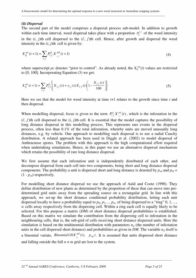
(ii) Dispersal The second part of the model comprises a dispersal process sub-model. In addition to growth

within each time interval, weed dispersal takes place with a proportion '' jiijP of the weed intensity

in the (i, j)th cell dispersed to the (i', j')th cell. Hence, after growth and dispersal the weed intensity in the (i, j)th cell is given by:

∑ +=+''

'' )1()1(''

ji

pdijji

pcij tXPtX

ji (4)

where superscript pc denotes “prior to control”. As already noted, the Xij

pc(t) values are restricted to [0, 100]. Incorporating Equation (3) we get:

∑

−+=+

''

''''''''''

100

)(1)()()()1(

ji

ji

jijijiijji

pcij

tXtXtrtXPtX (5)

Here we see that the model for weed intensity at time t+1 relates to the growth since time t and then dispersal.

When modelling dispersal, focus is given to the term )('''' tXP pdij

ji ji, which is the infestation in the

(i', j')th cell dispersed to the (i, j)th cell. It is essential that the model captures the possibility of long distance dispersal in this modelling process. This represents rare events in the dispersal process, often less than 0.1% of the total infestation, whereby units are moved unusually long distances, e.g. by vehicle. One approach to modelling such dispersal is to use a radial Cauchy distribution. A related approach has been used in Diggle et al. (2002) to model dispersal of Anthracnose spores. The problem with this approach is the high computational effort required when undertaking simulations. Hence, in this paper we use an alternative dispersal mechanism which retains the possibility of rare long distance dispersal. We first assume that each infestation unit is independently distributed of each other, and decompose dispersal from each cell into two components, being short and long distance dispersal components. The probability a unit is dispersed short and long distance is denoted by psd and pld = (1 - psd) respectively. For modelling short distance dispersal we use the approach of Auld and Coote (1990). They define distribution of new plants as determined by the proportion of these that can move into pre-determined grid units away from the spreading source on a rectangular grid. In line with this approach, we set-up the short distance conditional probability distribution, letting each unit dispersed locally to have a probability equal to p0, p1, ... pw, of being dispersed to a “ring” 0, 1, ..., w cells away respectively from the dispersing cell. Within a ring each cell is equally likely to be selected. For this purpose a matrix (DM) of short distance dispersal probabilities is established. Based on this matrix we simulate the contribution from the dispersing cell to infestation in the neighbouring cells, that is, the sub-grid of cells receiving short distance dispersed units. Here the simulation is based on the multinomial distribution with parameters nij (the number of infestation units in the cell dispersed short distance) and probabilities as given in DM. The variable nij itself is

a binomial variate, )),(10( sdpd

ptXBinomialij

. It is assumed that units dispersed short distance

and falling outside the full n × m grid are lost to the system.


_______________________________________________________________________________________

52 nd


The remaining units, ))(10( ijpd

ntXij

− , are distributed long distance. Each long distance

dispersed unit is then assigned at random to one of the “long distance” cells of the grid, these being those cells of the grid that are the complement to the short distance cells. The probability of a unit being assigned to any particular long distance cell is set inversely proportional to the squared distance the cell is from the dispersing cell. These probabilities approximate the probabilities for a Cauchy distribution in the tails and hence the long distance dispersal approximates a radial Cauchy distribution. Currently DM, the matrix of short distance conditional probabilities, is established with a maximum number of rings equal to four so that a maximum of 81 cells (9 × 9 sub grid) receive short distance dispersal. It is also assumed that, on average, of the units dispersed short distance;

• 95% of infestation units remain within the dispersing cell itself,

• 2% move to the 8 neighbouring cells,

• 1.5% move to the next 16 neighbouring cells,

• 1% move to the next 24 neighbouring cells, and

• 0.5% move to the last 32 neighbouring cells away from the dispersing middle cell. These parameters can be readily changed to suit the need of a particular case study weed problem. It should be noted here that dispersal of weeds in arable fields has been studied in relatively few cases. A rule of thumb developed in a summary of dispersal data by Cousens and Mortimer (1995) and later adopted by Woolcock and Cousens (2000) is that in species without clear dispersal adaptations, half the seeds are distributed within a distance of half the height of the parent plant. While most seeds are likely to be dispersed short distances by passive means, it is possible for a small proportion of seeds to disperse considerable distances due to rare events such as gale force winds, birds, farm machinery etc. Some evidence of these rare events is presented in field experiments by Auld (1988) in which he found a single Avena fatua plant established at 14m from the nearest source in the second year. Rare long-distance dispersal events are critically important in invasions and plant migration (Higgins et al., 1996; Higgins & Richardson, 1999). The conclusions drawn by Higgins and Richardson (1999) are that data on rare long-distance dispersal will remain (by definition) hard to come by, and that the rare long-distance dispersal component of the model can, if sufficiently rare, be estimated independently of the local dispersal components. In their analysis, they suggest that relatively large errors in estimating the long distance dispersal component are unlikely to strongly influence the predicted spread rate. Hence, it may be that accurate characterization of the long distance dispersal component is not as important as its identification. Accordingly, the spread modelling as discussed in this paper has incorporated both short and long distance weed spread. As shown in Figure 1, the new weed infestation starts in the middle of the grid field and spreads along the two dimensional fields (both length and breadth). Much of the spread takes place from the short distance dispersal while a much lower level of spread occurs from the rare long distance dispersal of this mixed distribution spread model. The movement of the spreading weed populations on the grid space for a possible set of parameters is illustrated in Figure 2. The spreading population moves along two dimensional fields as a ‘wave’ of population density. The weeds ‘search and control effort’ is incorporated into this model as described in the next section.


_______________________________________________________________________________________

52 nd


Breadth

Length

Short-distance dispersal with higher probability

Long-distance dispersal with a much lower probability to

accommodate the rare events in the dispersal process

Initial source of infestation

Figure 1. Mixed distribution of weeds dispersal adopted in the model

Note: Bivariate distribution takes a two dimensional plane both along the length and the breadth of the field

0 20 40 60 80 100

0

20

40

60

80

100

After 10 years

Breadth

Le

ng

th

0 20 40 60 80 100

0

20

40

60

80

100

After 15 years

Breadth

Le

ng

th

Figure 2. Spreading weed populations on the grid space

Note: On 100 × 100 grid under parameterization given in Table 1 with r = 1.35 and pld = 0.1


_______________________________________________________________________________________

52 nd


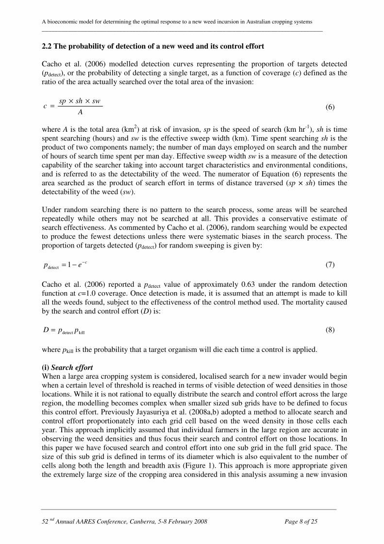
2.2 The probability of detection of a new weed and its control effort

Cacho et al. (2006) modelled detection curves representing the proportion of targets detected (pdetect), or the probability of detecting a single target, as a function of coverage (c) defined as the ratio of the area actually searched over the total area of the invasion:

A

swshspc

××= (6)

where A is the total area (km2) at risk of invasion, sp is the speed of search (km hr-1), sh is time spent searching (hours) and sw is the effective sweep width (km). Time spent searching sh is the product of two components namely; the number of man days employed on search and the number of hours of search time spent per man day. Effective sweep width sw is a measure of the detection capability of the searcher taking into account target characteristics and environmental conditions, and is referred to as the detectability of the weed. The numerator of Equation (6) represents the area searched as the product of search effort in terms of distance traversed (sp × sh) times the detectability of the weed (sw). Under random searching there is no pattern to the search process, some areas will be searched repeatedly while others may not be searched at all. This provides a conservative estimate of search effectiveness. As commented by Cacho et al. (2006), random searching would be expected to produce the fewest detections unless there were systematic biases in the search process. The proportion of targets detected (pdetect) for random sweeping is given by:

cep

−−= 1detect (7)

Cacho et al. (2006) reported a pdetect value of approximately 0.63 under the random detection function at c=1.0 coverage. Once detection is made, it is assumed that an attempt is made to kill all the weeds found, subject to the effectiveness of the control method used. The mortality caused by the search and control effort (D) is:

killdetect ppD = (8)

where pkill is the probability that a target organism will die each time a control is applied. (i) Search effort When a large area cropping system is considered, localised search for a new invader would begin when a certain level of threshold is reached in terms of visible detection of weed densities in those locations. While it is not rational to equally distribute the search and control effort across the large region, the modelling becomes complex when smaller sized sub grids have to be defined to focus this control effort. Previously Jayasuriya et al. (2008a,b) adopted a method to allocate search and control effort proportionately into each grid cell based on the weed density in those cells each year. This approach implicitly assumed that individual farmers in the large region are accurate in observing the weed densities and thus focus their search and control effort on those locations. In this paper we have focused search and control effort into one sub grid in the full grid space. The size of this sub grid is defined in terms of its diameter which is also equivalent to the number of cells along both the length and breadth axis (Figure 1). This approach is more appropriate given the extremely large size of the cropping area considered in this analysis assuming a new invasion


_______________________________________________________________________________________

52 nd


is discovered in a particular locality. Therefore shij for each (i, j)th cell across the n × m array (n =

m) in this newly defined sub grid at time t, is set proportional to Xijpc(t) so that shtsh

ij

ij =∑ )( .

(ii) Re-infestation from the soil seed bank Though a visible infestation can be killed after applying ‘search and control effort’ as shown in Equation 8, there is always the possibility of re-infestation occurring from the soil seed bank. Process-based demographic modelling such as Woolcock and Cousens (2000) has incorporated effective germination rates separately for new and old seeds in the seed bank. Literature citations on the seed germination rates vary for different weeds ranging from 25 to 50% for new and old seeds respectively in the case of Raphanus raphanistrum (wild radish), while it may be just 2% for Orobanche ramosa (branched broomrape) in field conditions. Due to the existing complexity of the spatial modelling framework, weed demography was not included as it would add considerably to the computational burden. Therefore, a more simplistic approach on incorporating weed re-infestation from the seed bank was required. We have re-adjusted the mortality caused by the search and control effort (D) to accommodate the re-infestation of weeds from the soil seed bank:

( )θ−= 1DM (9)

where M is mortality caused by the search and control effort after adjusting for the seed bank re-

infestation rate (θ ) where θ ∈ [0, 1]. To include dependence of M on cell (i, j) across the n × m array and on time t, Equation (9) can be written as:

[ ])(1)()( ttDtM ijijij θ−= (10)

Here θij(t) is set up to allow dependence on both cell and time. Replacing θij(t) with θ(t) would have the re-infestation parameter independent of space. In resembling the overall weed control effort in the defined sub grid field, this Mij(t) is then applied to Equation (5) to obtain:

[ ])(1)1()1( tMtXtX ij

pc

ijij −+=+ (11)

2.3 Damage functions associated with weed functional types

The presence of weeds results in damage to the grains cropping system. Damage in terms of crop yield loss (Z) is considered a proportional variable and is a function of the initial weed population in adult stages Xij(t) and the number of weeds killed expressed as the final mortality Mij(t), which is dependent upon the search and control parameters and the soil seed bank re-infestation rate as discussed above. Therefore,

[ ])(),()( tMtXftZ ij

pc

ijij = (12)

There are various functional forms that have been used to modelling damage functions in annual crops. Cousens (1985) and Martin et al. (1987) have assumed that yield loss is best represented by a rectangular hyperbola. The biological grounds for this argument are that at a low weed density, weeds are most competitive to crops and hence cause a maximum marginal reduction in crop yield. The effect of an increase in weed numbers at low densities is additive. However, when the density is high, increased intra-specific weed competition tends to reduce the marginal yield loss. This relationship dealing with intra-specific weed competition is appropriate for small scale


_______________________________________________________________________________________

52 nd


paddock level modelling. As this study involves a large regional scale modelling approach, a simple crop damage function is considered to be more applicable. For this purpose, a simple crop damage parameter is introduced and the crop yield is adjusted by this parameter whenever there is a weed invasion. This assumption of a simple linear crop damage function is said to be reasonable in the case of agriculture, where damage can be conveniently calculated as the difference in gross margins per hectare before and after the weed invades (Cacho, 2004). Hence, assuming a fixed crop damage function the damage in terms of crop yield loss for each (i, j)th cell at time t, [Zij(t)] is considered a fixed value. Yield (Y) is a function of the weed-free crop yield (Ywf) and crop damage (Z):

)1( ZYY wf −= (13)

Including dependence of Y on cell (i, j) across the n × m array and on time t, Equation (13) can be written as:

[ ])(1)()( tZtYtY ijijwfij −= (14)

2.4 Efficacy/performance of policy and management options Once the problem is well defined, the final stage is to make the decision on which management strategy (or combination of strategies) to use. A wide variety of both qualitative and quantitative processes are available for making such decisions. In some simple cases the choice of control (and how to implement it) may seem obvious. In more complicated scenarios, subjective or qualitative procedures such as multicriteria assessment may be useful, and optimization techniques also extend to more mathematically formal methods (Possingham, 1996). Cacho (2004) expressed the cost of weed control in terms of the target rate of spread as shown in Figure 3. The invasion is assumed to spread in a circular pattern and the size of the invasion is measured by its radius. The rate of spread can be slowed or reversed by targeting the invasion front. The decision as to attempt to eradicate the invasion is based on evaluating net benefits (benefits minus costs). The cost of slowing the weeds spread (control cost) is zero when the invasion is allowed to spread uncontrolled (vmax). As the target rate of spread decreases (with increased control intensity by moving left in Figure 3) the control cost increases. The cost function is expected to be convex to the origin as cheaper and easier control methods are used first, and more expensive options may be required for more intensive control. When the cost curve crosses the vertical axis, weed spread is stopped (total containment is achieved). When the rate of spread is negative, implying depletion in the weed seed bank, the invasion decreases with time and will eventually result in eradication. Partial control can slow the spread and although the entire area at risk will be eventually invaded, this option could have a value. Delaying the transition to a fully invaded environment means that benefits from the uninvaded area are obtained for a longer period and the costs of treatment are delayed. Slowing the spread also enhances the possibility of making eradication feasible if new technologies become available in the future.


_______________________________________________________________________________________

52 nd


Source : Cacho, 2004

Figure 3. The cost function for slowing the spread of weed invasion

The weed management policy is evaluated in a benefit-cost framework to evaluate the difference between the with-control and without-control options. The benefit cost ratio (BCR) is given by:

∑

∑

=

=

+

+−

=T

t

tt

T

t

tncwc

C

II

BCR

tt

1

1

)1/(

)1/()(

β

β

(15)

where Iwc and Inc are the incomes from the cropping enterprise under with-control and without-control respectively, C is the annual weed control cost and β is the discount rate. 2.5 Dynamic programming model.

The economic viability of different strategies in new weed incursion management is assessed in a multi-period context by employing a dynamic programming model linked to the weed spread simulation model described in section 2.1. The decision problem is to derive the optimal strategy for a new weed incursion in the Australian grains industry. The solution is the degree of incursion management strategy applied in each time period such that the net present value over the planning horizon is maximised. The problem is formulated by using the concepts of optimal control theory (Bellman, 1957). Dynamic programming is a computationally efficient method of solving such a problem and has been used by a number of studies for deriving optimal weed control strategies (eg, Fisher and Lee, 1981; Tayler and Burt, 1984; Pandey and Medd, 1990, 1991; Gorddard et al., 1995, 1996; Jones

Target rate of spread (v)

Cost of slowing the spread

0

no control Vmax

partial containment

total containment

eradication


_______________________________________________________________________________________

52 nd


and Medd, 1997, 2000; Cacho, 2004; and Jones, 2004). The specification of the model states, decision variables and profit function are now described. (i) State variables There are two state variables defined for the weed incursion management problem. The first is the size of the invasion (I) and the second is the budget available (B) for search and control. The invasion state is defined as the proportion of the total area invaded, and is comprised of 200 discrete values ranging from 0 to 100% infestation. An exponential equation is used to define the state values so as to give greater discrimination power at the critical lower invasion state levels. The set of invasion states was calculated as follows.

jj II ⋅=+ 0725.11 for j = 1, …, 200 (16)

{ }0.100,1.97,5.90,,00011.0,000107.0,00005.0,0000.0 L=I

In the dynamic programming model solution process, the proportional state variable is transformed into an area based variable as follows.

AI

IA ⋅=100

(17)

Where IA is the area invaded by new weed incursion (ha), and A is the area at risk of invasion (ha). This allows the computation of the non-invaded area (NA) in any year t.

tt IAANA −= (18)

The change in the invasion area state is a function of the intrinsic growth of weed spread (∆IA), and the area controlled (CA) due to the impact of search and control decisions.

tttt CAIAIAIA −∆+=+1 (19)

The annual increase in weed spread is obtained from a logistic growth equation, with the intrinsic growth parameter (σ) being obtained from solution of the weed spread model described in section 2.1.

−⋅=∆

A

IAIAIA t

tt 1σ (20)

The concept of a harvest function of a natural resource stock (Clark 1990) is used to represent the reduction in weed invasion area due to search and control efforts and is described in the decision variable section below. The budget state is included to account for any limits on public funds available for a weed eradication program. It is unlikely that funding for such a program would be unconstrained, either annually or in total. Consequently, two constraints are included in the model – the total budget and an annual funding limit. For this analysis there are 101 discrete budget states ranging from $0 to $50m.


_______________________________________________________________________________________

52 nd


{ }0.50,,0.1,50.0,0.0 K=B

The transition in the budget state is as follows.

ttt WCBB −=+1 (21)

( ) ( )( )[ ]COSTCOSTttCOSTCOSTt LCMCIApELFWC +⋅+⋅+= detect (22)

Where WC is the annual weed control costs ($), FCOST is fixed (administration) costs ($), LCOST is labour costs ($/day), E is the labour effort decision variable (man days), MCCOST is the cost of materials for control ($/ha) and LCCOST is the cost of labour for control ($/ha). The annual budget limit (BA) is defined by the following constraint.

BAWCt ≤ (23)

(ii) Decision variable There is a single control variable – the annual search and control effort (E) defined by the number of man days. The set of control decisions is defined as:

{ }50000,,5000,2500,0 K=E

As the effort devoted to searching for weed infestations increases there is a corresponding increase in the probability of detection. This is directly derived within the dynamic programming model by amending the coverage variable in Equation (6) as follows. The derivation of pdetect, and M remain as given in Equations (7) and (10).

( )

area

tt

S

swshEspc

⋅⋅⋅= (24)

The search area (ha), Sarea, is a user defined variable. Increasing the area to be searched for a given level of E reduces coverage and consequently the probability of detection. However, setting too small a search area means that some infestations may lie outside the search area and miss detection entirely. (iii) Stage

The stages modelled are production years. The planning horizon (T) consists of 50 years. (iv) Profit function The stage return is measured as the profit (π) from the grains enterprise from both the non-invaded and the invaded areas within the total cropping region.

( )( )[ ] [ ] twfctwfctt WCVCYPNALRVCZYPIA −−⋅+−−⋅⋅= ,1maxπ (25)

Where Pc is crop price ($/t), Ywf is weed-free yield (t/ha), Z is the crop damage factor, VC is crop variable costs ($/ha), and LR is livestock returns ($/ha). The opportunity cost of a new weed incursion is explicitly taken into account by including the variable LR which represents the returns from a livestock alternative. Consequently, if the post invasion return per hectare is less than LR, this alternative land use option is used in the profit function calculation. This condition is included so as to reduce the potential for overestimating the benefits of a weed control program.


_______________________________________________________________________________________

52 nd


The objective of the dynamic programming model is to maximise the net present value (NPV) of returns from the area (A) over the 50 year planning horizon. The recursive equation is given as follows.

( ) ( ) ( )[ ]111 ,,max, ++++= tttttu

ttt BIAVBIABIAVt

δπ (26)

Where Vt(·) is the maximum present value of returns from both invaded and non-invaded areas from year t to the end of the planning horizon, ut is the decision variable (ie. Et), π(IAt ,Bt) is the immediate return associated with ut decision alternative, and δ is the discount factor (1/(1+β))

where β is the discount rate. It is assumed that the terminal value equals zero, i.e. at t = 50, Vt+1(·) = 0. The solution of the recursive equation provides the optimal policy which indicates the level of control (ut) and NPV of returns for all combinations states and stages for any given size of invasion (IAt). Associated with the optimal control is the optimal state transition IAt � IAt+1 which indicates whether the invasion area increases (IAt < IAt+1), decreases (IAt > IAt+1) or remains stable (IAt = IAt+1) when subject to the optimal control.

3. Data for case study simulations Equation (2) is used to determine different values for the intrinsic growth rate parameter r. This value was computed for six hypothetical case study spread scenarios, being 4, 7, 10, 15, 20 and 30 years to reach a 95% infestation level, defined by the variable N. Parameter values for N and the resulting r value are given in Table 1. The conditional short distance probabilities p0, p1, ... p4 of being dispersed to 0, 1, ..., 4 cells away

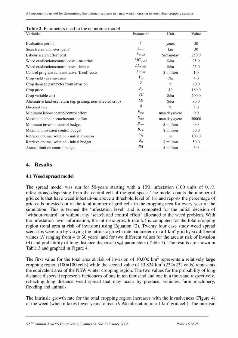
are given in Table 1. The parameters pkill and θ vary each year representing seasonal climatic variability. The parameters sp and sw vary for each grid cell and year, representing variability of search parameters on individual localities or search operations and the climate. Random variation is incorporated into these four parameters (i.e., weed control effort) in the form of a triangular probability distribution. In this way, for every model run, a particular parameter can assume a random value between the minimum and the maximum but mostly assumes the mode value as given in Table 1. Parameter values used in the economic model are given in Table 2. The time spent searching, as denoted by sh in Equation (6), was the decision variable on the weed control strategy and is expressed in ‘man days’ assuming 7 hours of search and control time spent per man day in the field.


_______________________________________________________________________________________

52 nd


Table 1. Parameters used in the weed spread model Variable Parameter Value

Total area at risk of invasion (km2) grid of 100 × 100 cells grid of 232 × 232 cells

A 10,000 53,824

Intrinsic growth rate when N years taken to reach 95% infestation, starting with a 0.1% infestation in 1 km2 grid cell: N = 30 N = 20 N = 15 N = 10 N = 7 N = 4

r

0.36 0.57 0.80 1.35 2.38 9.19

Probability of long distance dispersal (%) pld 0.10 0.01

Conditional short distance dispersal probabilities: (%) probability of dispersal: within the dispersing cell itself among the 8 cells lying around one cell away among the 16 cells lying around two cells away among the 24 cells lying around three cells away among the 32 cells lying around four cells away

p0

p1

p2

p3

p4

95.0 2.0 1.5 1.0 0.5

Speed of search (km/hr) – minimum value – mode value – maximum value

sp 0.90 1.00 1.05

Effective sweep width (km) – minimum value – mode value – maximum value

sw 0.018 0.020 0.021

Probability of kill each time control is applied (%) – minimum value – mode value – maximum value

pkill 70.0 95.0 97.0

Re-infestation rate from the soil seed bank (%) – minimum value – mode value – maximum value

θ 20.0 25.0 30.0


_______________________________________________________________________________________

52 nd


Table 2. Parameters used in the economic model Variable Parameter Unit Value

Evaluation period T years 50

Search area diameter (cells) Sarea km 30

Labour search effort cost LCOST $/man/day 250.0

Weed eradication/control costs - materials MCCOST $/ha 25.0

Weed eradication/control costs - labour LCCOST $/ha 25.0

Control program administrative (fixed) costs FCOST $ million 1.0

Crop yield - pre-invasion Ywf t/ha 4.0

Crop damage parameter from invasion Z % 60.0

Crop price Pc $/t 180.0

Crop variable cost VC $/ha 200.0

Alternative land-use return (eg. grazing, non-affected crop) LR $/ha 80.0

Discount rate β % 5.0

Minimum labour search/control effort Emin man days/year 0.0

Maximum labour search/control effort Emax man days/year 50000

Minimum invasion control budget Bmax $ million 0.0

Maximum invasion control budget Bmin $ million 50.0

Retrieve optimal solution - initial invasion IA0 ha 100.0

Retrieve optimal solution - initial budget B0 $ million 50.0

Annual limit on control budget BA $ million 5.0

4. Results 4.1 Weed spread model

The spread model was run for 50-years starting with a 10% infestation (100 units of 0.1% infestations) dispersing from the central cell of the grid space. The model counts the number of grid cells that have weed infestations above a threshold level of 1% and reports the percentage of grid cells infested out of the total number of grid cells in the cropping area for every year of the simulation. This is termed the ‘infestation level’ and is computed for the initial decision of ‘without-control’ or without any ‘search and control effort’ allocated to the weed problem. With the infestation level information, the intrinsic growth rate (σ) is computed for the total cropping region (total area at risk of invasion) using Equation (2). Twenty four case study weed spread scenarios were run by varying the intrinsic growth rate parameter r in a 1 km2 grid by six different values (N ranging from 4 to 30 years) and for two different values for the area at risk of invasion (A) and probability of long distance dispersal (pld) parameters (Table 1). The results are shown in Table 3 and graphed in Figure 4. The first value for the total area at risk of invasion of 10,000 km2 represents a relatively large cropping region (100×100 cells) while the second value of 53,824 km2 (232×232 cells) represents the equivalent area of the NSW winter cropping region. The two values for the probability of long distance dispersal represents incidences of one in ten thousand and one in a thousand respectively, reflecting long distance weed spread that may occur by produce, vehicles, farm machinery, flooding and animals. The intrinsic growth rate for the total cropping region increases with the invasiveness (Figure 4) of the weed (when it takes fewer years to reach 95% infestation in a 1 km2 grid cell). The intrinsic


_______________________________________________________________________________________

52 nd


growth rate also increases with a higher probability of long distance dispersal. The weed spread is less in terms of the proportion of the area infested when the total cropping region is large compared to the smaller region. Table 3. Intrinsic growth rate for the total cropping region

A

(km2) pld

(%)

N=30

N=20 σ

N=15

N=10

N=7

N=4

10000 0.01 0.16 0.25 0.32 0.42 0.59 1.00

0.10 0.17 0.34 0.42 0.58 0.80 1.00

53824 0.01 0.12 0.20 0.24 0.33 0.42 0.80

0.10 0.12 0.27 0.33 0.45 0.62 1.00

Note: N is the number of years taken to reach 95% infestation in a 1 km2 grid cell.

100 x 100 km2 Area

0.0

0.1

0.2

0.3

0.4

0.5

0.6

0.7

0.8

0.9

1.0

N=30 N=20 N=15 N=10 N=7 N=4

Invasiveness

Intr

insic

gro

wth

rate

232 x 232 km2 Area

0.0

0.1

0.2

0.3

0.4

0.5

0.6

0.7

0.8

0.9

1.0

N=30 N=20 N=15 N=10 N=7 N=4

Invasiveness

Intr

insic

gro

wth

rate

Figure 4. Intrinsic growth rate for the total cropping region with the probability of long distance dispersal pld = 0.01 (—▲—) and pld = 0.10 (—�—)


_______________________________________________________________________________________

52 nd


4.2 Dynamic programming model

(i) Optimal decision rules The solution of the dynamic programming model provides the optimal decision rule for all possible states. A summary of the control effort decisions is given in Table 4 for a discrete set of invasion area states from 100 to 10000 ha. This indicates that the level of control effort increases with the size of the weed invasion. For example, for σ = 0.2 the optimal decision ranged from zero control effort at an infestation of 100 ha to 15000 man days a year for a 10000 ha invasion. The optimal level of control effort also increases with the invasiveness of the weed as represented by the results for σ values of 0.4 to 1.0 in Table 4. For the case of a 100 ha initial infestation it is optimal to implement control efforts of 7500, 10000, 12500 and 17500 man days a year respectively for σ values of 0.4, 0.6, 0.8 and 1.0. Table 4. Optimal weed search and control effort decisions at various invasion levels under different intrinsic growth rates (man days)

Invasion (ha) σ = 0.2 σ = 0.4 σ = 0.6 σ = 0.8 σ = 1.0

100 0 7500 10000 12500 17500 500 0 12500 10000 12500 12500

1000 7500 12500 10000 12500 12500 2000 7500 12500 10000 12500 12500 3000 10000 12500 15000 12500 12500 4000 10000 12500 15000 12500 20000 5000 10000 12500 15000 12500 20000 6000 10000 12500 15000 15000 20000 7000 15000 12500 15000 17500 20000 8000 15000 12500 15000 17500 20000 9000 15000 12500 15000 17500 20000

10000 15000 12500 15000 17500 20000

(ii) Impact on weed infestation area The impact upon the infestation area over the 50-year simulation period from following the optimal control decisions is illustrated in Figure 5 for the case of an initial infestation of 100 ha. The two scenarios of without-control and with-control program are plotted separately as in the latter case the infested area declined for all levels of weed invasiveness, whereas without-control the infested area increased. Without any control program the area of weed invasion would spread to 4.5m ha by year 45 and 5.0m ha by year 30 for σ values of 0.4 and 0.6 respectively. For σ values of 0.8 and 1.0 the rate of spread is increased. When a control program is implemented, the invasion is reduced to close to zero from an initial infestation of 100 ha within 6 to 8 years and all four intrinsic growth rates.


_______________________________________________________________________________________

52 nd


100 ha Starting Infestation - without control

0

1000000

2000000

3000000

4000000

5000000

6000000

1 8 15 22 29 36 43 50

Year

Infe

ste

d A

rea

(h

a)

100 ha Starting Infestation - with control

0

10

20

30

40

50

60

70

80

90

100

1 8 15 22 29 36 43 50

Year

Infe

ste

d A

rea (

ha)

Figure 5. Weed spread from initial infestation of 100 ha for without-control and with-control under different intrinsic growth rates σ = 0.4 (…….), σ = 0.6 (_ _ _ _ _ ) σ = 0.8 (─ - ─),

σ = 1.0 (——) (iii) Benefit-cost analysis

The outcomes of applying the optimal decision rules are incorporated into a benefit-cost analysis to determine the long-term benefits of a weed control program. Two initial weed invasion scenarios are evaluated; a relatively small invasion (100 ha) and a moderate sized invasion (1000 ha). The results of the benefit-cost analysis are given in Tables 5 and 6 for these two scenarios with a range of intrinsic growth rates. For an initial infestation of 100 ha the benefit-cost ratio (BCR) from a control program ranged from 7:1 for σ = 0.2 to 624:1 for σ = 0.8. The discounted benefits represent the difference in the annual income streams from the cropping area for with-control and without-control, and increase substantially with the degree of invasiveness of a weed. For example, the discounted benefits are $36m for the case of σ = 0.2, but reach $16806m for σ = 1.0. Clearly, there are significant benefits to be achieved by controlling highly invasive weeds when initial infestations are at a low level (eg. 100 ha). The benefit-cost analysis results for the case of an initial invasion of 1000 ha differ to the smaller infestation scenario. For the case of σ = 0.2 and 0.4, there is an increase in the BCR from implementing a weed control program. This is mostly due to a higher discounted benefit between the with-control and without-control compared to the 100 ha infestation scenario. However, the returns from a control program, as measured by the BCR, are less for the greater invasiveness conditions than can be achieved for the smaller initial infestation. For example, when σ = 0.8 the BCR is 461:1 for the 1000 ha invasion compared to 624:1 for the 100 ha invasion. The difference in the benefits of a control program for the two initial invasion scenarios is attributable to the impact of the budget state variable. For the smaller infestation, the budget state


_______________________________________________________________________________________

52 nd


is not limiting throughout the simulation. However, for some of the σ scenarios the budget does become a limiting factor due to the size of the invasion area that has to be searched and the cost of control. This is illustrated in Figure 6 where the path in the budget state variable is illustrated for the two initial invasion scenarios and for three intrinsic growth rates 0.4, 0.8 and 1.0. This indicates that for the larger initial invasion and σ = 0.8 and 1.0 the weed control budget is exhausted within 20-years. This then implies that the area of the invasive weed cannot be controlled, and the area of invasion subsequently increases. Therefore, the benefits of the weed control program are reduced because of the increasing area of weed spread. Table 5. Discounted benefits, costs and benefit-cost ratio of weed control under different intrinsic growth rates for an initial infestation of 100 ha ($m)

σ = 0.2 σ = 0.4 σ = 0.6 σ = 0.8 σ = 1.0

Discounted benefits 36 3402 9200 14582 16806 Discounted costs 5 17 20 23 30 Benefit-cost ratio 7:1 204:1 452:1 624:1 563:1

Table 6. Discounted benefits, costs and benefit-cost ratio of weed control under different intrinsic growth rates for an initial infestation of 1000 ha ($m)

σ = 0.2 σ = 0.4 σ = 0.6 σ = 0.8 σ = 1.0

Discounted benefits 391 6731 13153 14395 13957 Discounted costs 13 28 32 31 33 Benefit-cost ratio 31:1 244:1 409:1 461:1 420:1

(a) 100 ha Starting Infestation - with control

0

10

20

30

40

50

1 8 15 22 29 36 43 50

Year

Bu

dg

et

Availab

le (

$ m

il)

(b) 1000 ha Starting Infestation - with control

0

10

20

30

40

50

1 8 15 22 29 36 43 50

Year

Bu

dg

et

Availab

le (

$ m

il)

Figure 6. The path of the budget state variable for initial infestations of 100 and 1000 ha under

different intrinsic growth rates of σ = 0.4 (…….), σ = 0.8 (─ - ─) and σ = 1.0 (——)


_______________________________________________________________________________________

52 nd


(iv) Sensitivity analysis Sensitivity analysis was undertaken on a number of potentially important model variables to determine the difference in the benefit-cost analysis for an initial weed incursion of 100 ha. The variables considered were the probability of weed kill (pkill), the re-infestation rate from the soil

seed bank (θ), the labour search effort cost (Lcost), the crop damage parameter from invasion (Z) and the discount rate (β). The results of a 10% change of these individual variables are presented in Table 7 (σ = 0.4) and Table 8 (σ = 0.8). Decreasing the pkill by 10% resulted in a substantial increase in discounted costs by 20% and 46% when σ = 0.4 and 0.8 respectively. The higher change under high invasive scenario is due to the higher costs involved in the control of a fast spreading weed after lowering the probability of kill in the control program. Due to these changes the respective benefit-cost ratios decreased by 17% and 31% for the two σ scenarios.

Increasing θ by 10% resulted in increased discounted costs by 3% and 14% when σ = 0.4 and 0.8 respectively. This implies the impact of a higher seed bank re-infestation on weed control cost is high if the weed is of high invasive type while the impact is less for the low invasive types. The resulting effect on benefit-cost ratio is a decrease by the same magnitude for the two σ scenarios. Increasing Lcost by 10% resulted in increased discounted costs and therefore decreased benefit-cost ratios by the same magnitude of between 7 and 8% for both σ scenarios. The damage in terms of yield loss from a 100 ha initial infestation is very low given the returns from a total cropping region of 53,824 km2 (232×232 grid) considered in this case study analysis. Therefore a 10% change in crop damage parameter (Z) has not shown any effect on the benefits and costs, but changes could be expected in a larger infestation. The effect of 10% increase of discount rate (β) resulted in decreased benefits at a higher magnitude (14-18%) but decreased costs at a much lower magnitude (1-2%). The significant benefits achieved by weed control in terms of higher incomes in future years are reduced in terms of present value of these income streams when a higher discount rate is used. The overall result is the decrease in benefit-cost ratio by more than the change in β. Table 7. The impact on the benefit-cost analysis of 10% variation to key model parameters (σ =

0.4)

Discounted benefits

($m) Discounted costs

($m) Benefit-cost ratio

($m)

Base 3402 17 204:1

pkill = 85.5% (-10%)

3402 (0%)

20 (+20%)

169:1 (-17%)

θ = 27.5% (+10%)

3402 (0%)

17 (+3%)

198:1 (-3%)

Lcost = 275 $/man day

(+10%) 3402 (0%)

18 (+7%)

190:1 (-7%)

Z = 66% (+10%)

3402 (0%)

17 (0%)

204:1 (0%)

β = 5.5% (+10%)

2794 (-18%)

16 (-1%)

170:1 (-17%)


_______________________________________________________________________________________

52 nd


Table 8. The impact on the benefit-cost analysis of 10% variation to key model parameters (σ =

0.8)

Discounted benefits

($m) Discounted costs

($m) Benefit-cost ratio

($m)

Base 14582 23 624:1

pkill = 85.5% (-10%)

14582 (0%)

34 (+46%)

427:1 (-31%)

θ = 27.5% (+10%)

14582 (0%)

27 (+14%)

546:1 (-12%)

Lcost = 275 $/man day

(+10%) 14582 (0%)

25 (+8%)

579:1 (-7%)

Z = 66% (+10%)

14582 (0%)

23 (0%)

624:1 (0%)

β = 5.5% (+10%)

12593 (-14%)

23 (-2%)

548:1 (-12%)

5. Conclusion In this paper we presented a bioeconomic simulation framework with a mathematical model representing weed spread linked to a dynamic programming model providing a means of determining the economically optimal weed management strategies over time. Development of this bioeconomic model was funded by the Cooperative Research Centre for Australian Weed Management to assist decision makers to determine the economically optimal strategies for dealing with new weed incursions in cropping systems. This model could be applied to large area cropping systems such as its current application to the NSW wheat growing region and where long distance weed spread can occur due to vehicles, farm machinery, flood or by animals such as bird dispersal. The spread model has modest data requirements (for a spatial simulation model) in that it concentrates on simulating population growth, dispersal processes and mortality (including search and control) and ignores the environmental and biotic heterogeneity of the receiving environment. With the dynamic programming model it is possible to assess economic viability of different weed management strategies in a multi-period context as in the case of many resource management problems requiring decisions which are sequential, risky and irreversible. The modelling framework was used to evaluate case study invasive weed control problems in the Australian grains industry. The intrinsic growth rate for the total cropping region increases with the invasiveness of the weed. It is also higher with a higher probability of long distance dispersal. The weed spread is slow when the total cropping region is large compared to a smaller region. The model indicates that the level of control effort defined in terms of labour devoted to search and control increases with the size of the weed invasion. The optimal level of control effort also increases with the invasiveness of the weed as represented by its intrinsic growth rate. The outcomes of applying the optimal decision rules were incorporated into a benefit-cost analysis to determine the long-term benefits of a weed control program. The discounted benefits represent the difference in the annual income streams from the cropping area for with-control and without-control, and increase substantially with the degree of invasiveness of a weed. Clearly, there are significant benefits to be achieved by controlling highly invasive weeds when initial infestations are at a low level. The cost of weed control also increases with invasiveness, but the magnitude of this is smaller compared to the increased benefits received. As a result the increase in the benefit-cost ratio is very high under high invasive weed infestation control.


_______________________________________________________________________________________

52 nd


The benefit-cost ratios are generally very high, regardless of whether the control budget has run out or not. For small infestations (at least up to 1000 ha) it is economical to eradicate weeds with a range of invasiveness. Even if the invasion cannot be eradicated due to its high invasiveness or budget constraints, still it pays to maintain invasions at lower level. This is in line with the work by Sharov and Liebhold (1998) and Cacho (2004) which showed that slowing population spread is a viable strategy of invasion control while the optimal strategy changes from eradication to slowing the spread to finally doing nothing. In future work we intend to elaborate on this aspect and analyse a comprehensive range of benefit-cost scenarios across a broad range of initial invasions and intrinsic growth rates to identify these ‘switching points’. Lowering the model variable ‘probability of weed kill’ or increasing ‘re-infestation rate from the soil seed bank’ or ‘labour search effort cost’ results in increasing discounted costs and therefore decreasing the benefit-cost ratio. The damage in terms of yield loss from a 100 ha initial infestation is very low given the returns from an extremely large total cropping region considered in this case study analysis. Therefore a change in crop damage parameter has not shown any effect on the benefits and costs, but changes could be expected from a larger infestation. The effect of an increased discount rate results in decreased benefits at a higher magnitude and decreased costs at a much lower magnitude resulting in a higher decrease in benefit-cost ratio from weed control.

References Auld, B.A. (1988). Dynamics of pasture invasion by three weeds, Avena fatua L., Carduus

tenuiflorus Curt. And Onopordum acanthium L., Australian Journal of Agricultural Research 39, 589-596.

Auld, B.A. and Coote, B.G. (1990). INVADE: Towards the simulation of plant spread, Agriculture, Ecosystems and Environment 30, 121-128.

Bellman, R.E. (1957). Dynamic Programming. Princeton University Press, Princeton, New Jersey.

Buhler, D.D., King, R.P., Swinton, S.M., Gunsolus, J.L. and Forcella, F. (1996). Field evaluation of a bioeconomic model for weed management in corn (Zea mays), Weed Science 44, 915-923.

Buhler, D.D., King, R.P., Swinton, S.M., Gunsolus, J.L. and Forcella, F. (1997). Field evaluation of a bioeconomic model for weed management in soybean (Glycine max), Weed Science 45, 158-165.

Cacho, O.J. (2004). When is it optimal to eradicate a weed invasion? In Sindel, B.M. and Johnson, S.B. (eds), 14

th Australian Weeds Conference papers & proceedings, 6-9 September

2004, Wagga Wagga, New South Wales, Australia, pp. 49-54. Cacho, O.J., Spring, D., Pheloung, P. and Hester, S. (2006). Evaluating the feasibility of

eradicating an invasion, Biological Invasions 8, 903-917. Clark, C.W. (1990). Mathematical Bioeconomics: The Optimal Management of Renewable

Resources. Second Edition, John Wiley & Sons, Inc., New York, USA. Cousens, R. (1985). An empirical model relating crop yield to weed and crop density and a

statistical comparison with other models, The Journal of Agricultural Science 105, 513-521. Cousens, R. and Mortimer, M. (1995). Dynamics of Weed Populations. Cambridge University

Press, Cambridge, UK. Diggle, A.J., Salam, M.U., Thomas, G.J., Yang, H.A., O’Connell, M. and Sweetingham, M.W.

(2002). Anthracnose Tracer: A Spatiotemporal Model for Simulating the Spread of Anthracnose in a Lupin Field, Phytopathology 92(10), 1110-1119.

Fisher, B.S. and Lee, R.R. (1981). A dynamic programming approach to the economic control of weed and disease infestations, Review of Marketing and Agricultural Economics 49, 175-187.


_______________________________________________________________________________________

52 nd


Gorddard, R.J., Pannell, D.J. and Hertzler, G. (1995). An optimal control model for integrated weed management under herbicide resistance, Australian Journal of Agricultural Economics 39(1), 71-87.

Gorddard, R.J., Pannell, D.J. and Hertzler, G. (1996). Economic evaluation of strategies for management of herbicide resistance, Agricultural Systems 51, 281-298.

Higgins, S.I. and Richardson, D.M. (1999). Predicting plant migration rates in a changing world: the role of long-distance dispersal, American Naturalist 153, 464–475.

Higgins, S.I., Richardson, D.M. and Cowling, R.M. (1996). Modelling invasive plant spread: The role of plant-environment interactions and model structure, Ecology 77, 2043-2054.

Jayasuriya, R.T., Van de ven R., and Jones, R. (2008a forthcoming). Spatial modelling of new weed incursions in cropping systems. Paper accepted for the 16th Australian Weeds

Conference, 18-22 May 2008, Cairns, North Queensland, Australia. To be published in an edited volume of conference proceedings.

Jayasuriya, R.T., Van de ven R., and Jones, R. (2008b submitted). Mathematical modelling of a new weed incursion and its control in large area cropping systems. Paper submitted to the Weed Research Journal.

Jones, R. (2004). The economic benefits of IWM: the role of risk and sustainability in farming systems. In Sindel, B.M. and Johnson, S.B. (eds), 14

th Australian Weeds Conference papers

& proceedings, 6-9 September 2004, Wagga Wagga, New South Wales, Australia, pp. 576-579.

Jones, R. and Medd, R. (1997). Economic analysis of integrated management of wild oats involving fallow, herbicide and crop rotational options, Australian Journal of Experimental

Agriculture 37, 683-691. Jones, R.E. and Medd, R.W. (2000). Economic thresholds and the case for longer term approaches

to population management of weeds, Weed Technology 14, 337-350. Kwon, T., Young, D.L., Young, F.L. and Boerboom, C.M. (1995). PALWEED WHEAT: a

bioeconomic decision model for postemergence weed management in winter wheat (Triticum aestivum), Weed Science 43, 595-603.

Lonsdale, W.M. (1993). Rates of spread of an invading species – Mimosa pigra in Northern Australia, Journal of Ecology 81, 513-521.

Martin, R.J., Cullis, B.R. and McNamara, D.W. (1987). Prediction of wheat yield loss due to competition by wild oats (Avena spp.), Australian Journal of Agricultural Research 38, 487-499.

Martin, A.R., Mortensen, D.A. and Lindquist, J.L. (1998). Decision support models for weed management: In-field management tools. In Hatfield, J.L., Buhler, D.D. and Stewart, B.A. (eds), Integrated weed and soil management, Ann Arbor Press, Michigan, USA, pp. 363-369.

Pandey, S. and Medd, R.W. (1990). Integration of seed and plant kill tactics for control of wild oats: an economic evaluation, Agricultural Systems 34(1), 65-76.

Pandey, S. and Medd, R.W. (1991). A stochastic dynamic programming framework for weed control decision making: an application to Avena fatua L., Agricultural Economics 6(2), 115-128.

Possingham, H.P. (1996). Decision theory and biodiversity management: How to manage a metapopulation. In Floyd, R.B., Sheppard, A.W. and De Barro, P.J. (eds), Frontiers of

Population Ecology, CSIRO Publishing, Melbourne, pp. 391 398. Schweizer, E.E, Lybecker, D.W. and Wiles, L.J. (1998). Important biological information needed

for bioeconomic weed management models. In Hatfield, J.L., Buhler, D.D. and Stewart, B.A. (eds), Integrated weed and soil management, Ann Arbor Press, Michigan, USA, pp. 1-24.

Sharov, A.A. and Liebhold, A.M. (1998). Bioeconomics of managing the spread of exotic pest species with barrier zones, Ecological Applications 8(3), 833-845.


_______________________________________________________________________________________

52 nd


Sinden, J., Jones, R., Hester, S., Odom, D., Kalisch, C., James, R. and Cacho, O. (2004). The

economic impact of weeds in Australia. CRC for Australian Weed Management, Technical Series, No 8, Adelaide.

Tayler, C.R. and Burt, O.R. (1984). Near optimal management strategies for controlling wild oats in spring wheat, American Journal of Agricultural Economics 66, 50-60.

Woolcock, J.L. and Cousens, R. (2000). A mathematical analysis of factors affecting the rate of spread of patches of annual weeds in an arable field, Weed Science 48, 27-34.

a bioeconomic model for determining the optimal response...

Documents