a bernstein polynomail root solver

A BERNSTEIN POLYNOMAIL ROOT SOLVER

A Dissertation Presented to the

Department of Computer Science University of Sheffield

In partial fulfillment Of the Requirements of Degree

MSc Advance Software Engineering

By

Kiran Kanth Damaraju

Under the supervision of

Dr. Joab Winkler

August 2004

DECLARATION

All sentences or passages quoted in this dissertation from other people's work have been specifically acknowledged by clear cross-referencing to author, work and page(s). Any illustrations which are not the work of the author of this dissertation have been used with the explicit permission of the originator and are specifically acknowledged. I understand that failure to do this amounts to plagiarism and will be considered grounds for failure in this dissertation and the degree examination as a whole. Name: Kiran Kanth Damaraju Signature: Date:27/08/2004

ABSTRACT

The objective of this dissertation is to develop a Matlab suite to approximate all the real roots and multiplicities of univariate polynomial expressed in Bernstein basis over the unit interval. Approximation of real roots of Bernstein form polynomials over the unit interval has several applications in CAGD (Computer Aided Graphics Design). Several algorithms for approximating the real roots of Bernstein form polynomials have been proposed over years. This dissertation develops the Matlab suite based on the Bernstein Convex Hull Approximation Algorithm to approximate the roots of the Bernstein form polynomials over the unit interval. And also implements s some steps to improve the accuracy of the roots and to find the multiplicities of the roots.

i

ACKNOWLEDGEMENTS This project has benefited from the help and support of many people. Through out the project they offered constant help, guidance and receptive to my every need. I would like to thank my project supervisor Dr. Joab Winkler for offering the project of my choice and for his constant supervision and help during the period of project, which helped me to finish the project on time. I would like to thank all my friends, who knowingly or unknowingly have helped me with the project. A special thanks to all at my home, my Dad, Mom, Brother and Sister who have been encouraging me every day of my stay here. A special thanks to Vamsi Chunduru and Pradeep Konikanti for testing the project and providing the valuable feed back.

ii

CONTENTS 1 Introduction 1

1.1 Overview…………………………………………… 3 2 Review of Bernstein form Polynomials 4

2.1 Bernstein Basis …………………….. ……………. 5 2.2 Properties of Bernstein Basis…………………….... 7

2.2.1 Bernstein basis polynomials are recursively defined……7 2.2.2 All Bernstein polynomials are non-negative over [0,1]…8

2.2.3 All Bernstein polynomials for partition of unity……. 8

2.2.4 Bernstein polynomials can be expressed in power basis. 9

2.2.5 Degree Raising……………………………………… 10

2.3 Explicit Bézier Curves…………………………… 11

2.3.1 Convex Hull Property…………………………….. 11 2.3.2 Variation Diminishing Property…………………. 11

3 Review of Preconditioning and Real Root Finding Algorithms 13

3.1 Preconditioning for Bernstein form Polynomials… 13

iii

3.2 Polynomial Approximation algorithms…………… 16 3.2.1 Recursive Subdivision Techniques…………………… 16 3.2.2 Newton-based Techniques……………………………. 18 3.2.3 Hull Approximation Techniques…………………….… 19

4 Bernstein Polynomial Root Finding Concepts 20

4.1 Coefficient Normalization…………………….….. 21 4.2 Evaluation of Bernstein Polynomials…………….. 23

4.3 Bernstein Subdivision…………………………….. 25

4.3.1 de Casteljau Algorithm……………………………… 26

4.4 Bernstein Deflation………………………………… 28 4.5 Bernstein Differentiation…………………………. 30

5 Polynomial Approximation Algorithm 33

5.1 Bernstein Convex Hull Approximation Method… 33

5.1.1 Approximation step……………………………….. 34 5.1.2 BCH Algorithm…………………………………… 36

5.1.3 Modified BCH Algorithm………………………… 39

6 Numerical Results and Discussion 41 7 Conclusion 46

iv

Chapter 1

Introduction The objective of this dissertation is to develop a set of MATLAB programs to approximate all the real roots of a univariate polynomial expressed in Bernstein form over unit interval. Polynomials expressed in Bernstein form have grater applications in CAGD (Computer Aided Geometric Design). They are used for the designing of curves and serve as a basis for many generalizations. CAGD was coined by R. Barnhill and R. Riesenfeld in 1974 at a conference held at the University of Utah. Many of the Geometric Modeling problems concerned with the algebraic curves and surfaces can be reduced through the elimination methods to determine the real roots of a univariate polynomial on a bounded interval [FR 87]. Bernstein polynomials were originally introduced in [Bernstein’12] by S.N. Bernstein for the approximation of continuous function over a specified interval. The importance of Bernstein polynomials for CAGD comes from the ability to express Bézier curves and surfaces in the form of Bernstein form polynomials. This ability reduces many of the Bézier intersection problems to approximating real roots of Bernstein form polynomials. A well known application of Bernstein form polynomials to CAGD is to find the intersection points of two Bézier curves [SP 86]. The problem of finding the intersection point of Bézier curves of degree and degree n can be reduced to the problem of finding roots of the Bernstein polynomial of degree

mm n× . Similar applications include finding

the intersection points on each intersection loop of two Bézier surfaces [Far 86], ray-tracing tracing parametric surface patches, algebraic surface rendering [Sed 85] and trimming of bisector curves [FJ 94]. While explaining about the importance of Bernstein-Bézier patches, G.Frain in one of his papers [Fra 84] claimed, “The rapidly growing Field of CAGD has been dominated by the theory of the rectangular surface patches” and also mentioned “the Bernstein-Bézier methods help to give meaning to the ‘G’ in CAGD”.

1

CHAPTER 1. Introduction The polynomials resulting from the elimination process are usually of a much higher degree than the geometric entities being solved, and the coefficients of the polynomials derived from computationally extensive procedures. If such computations are performed in finite precision arithmetic, round off errors affect the coefficients of the polynomials. But the roots of polynomials have to be stable for these perturbations in the coefficients. So, the polynomial basis that is less sensitive to the perturbations in the coefficients has to be chosen. In early days, to find the root of Bernstein polynomials, they were converted into power basis and solved using the traditional root solving methods because of their familiarity. However, later, root solving algorithms have been developed for polynomials in Bernstein form itself. This is because both the empirical [FR 87] and analytical [FR 87, FR 88] results proved that polynomials expressed in Bernstein form are not only stable but also better root conditioned than polynomials in power form. Another advantage of Solving Bernstein form polynomials is the representation of Bernstein polynomials as explicit Bézier curves. This gives the advantage of using the convex hull property of Bézier curve in solving the roots of the polynomial. It has been proved that these root finding techniques are faster and more accurate than the traditional root finding methods for power basis [Spe 94]. This dissertation concentrates on the “Bernstein Convex Hull Approximation Step” algorithm [Spe 94] for finding the roots of Bernstein polynomial and proposes a modified form of this algorithm, though few other algorithms exist.

2

CHAPTER 1. Introduction

1.1 Overview Chapter 2 reviews the polynomials in Bernstein form and Bernstein basis functions. It also describes the properties of Bernstein Basis Polynomials and explains the numerical conditions of Polynomials in Bernstein form.

Chapter3 reviews the preconditioning of Bernstein form polynomials and outlines some of the techniques that have been proposed for approximating the roots of a Bernstein form polynomial over unit interval.

Chapter 4 discusses the theories used by most of the root solving algorithms for Polynomials in Bernstein form such as Evaluation, Subdivision, Normalization, Differentiation and Deflation techniques in detail. It also provides the mat lab implementation of these techniques.

Chapter 5 outlines the various root solving algorithms for polynomials in Bernstein form and discusses the Bernstein Convex Hull Approximation Algorithm in detail.

Chapter 6 presents the results of empirical testing of the algorithm proposed in the previous chapter and discusses the results.Chapter7 Concludes and summarizes this work.

3

Chapter 2

Review of Bernstein form Polynomials A degree n univariate Bernstein polynomial over interval [a, b] is expressed as

( ) ( ) ( )[ , ]

0 ( )

n k knn

a b k k nk

b t t ay y

b a

−

=

− −=

−∑ (2.1)

where are the Bernstein coefficients. In most of the applications of Bernstein

polynomials, the interval of interest is [0, 1]. Therefore substituting [0, 1] in place of [a, b] in the above equation gives

ky

(2.2) ( )[0,1]0

(1 )n

n nk k

k

y y t −

=

= −∑ k kt

k k

subscript [0, 1] at the bottom of y indicates the domain of interest. The term

is the Bernstein basis function of degree n. ( ) (1 )n nk t t−−

The section [§2.1] explains about the Bernstein basis function, section [§2.2]

discusses the properties associated with the Bernstein basis function and section [§2.3] explains about the explicit Bézier curves and some of the important properties of this representation of Bézier curves.

4

CHAPTER 2. Review of Bernstein form Polynomials

2.1 Bernstein Basis A Bernstein polynomial of degree n is defined as

( ),!( ) (1 )

! !n k k

k nnB t t t

k n k−= −

− (2.1.1)

Where ( )

!! !

nk n k−

is a binomial function. There are n+1 Bernstein basis functions for

degree n Bernstein polynomial. We usually set , ( )i nB t =0 if 0i < or i n . >

These polynomials are quite easy to write down: the coefficients ( )

!! !

nk n k−

can be

obtained from Pascal’s triangle, the exponents on the t term increase by one as i increases and the exponents on the term decrease by one as i increases. (1 )t− The first few Bernstein polynomial basis function are expressed as

0,0

0,1

1,0

20,2

1,2

22,2

( ) 1( ) 1( )

( ) (1 )( ) 2( )(1 )

( )

B tB t tB t t

B t tB t t

B t t

t

=

= −

=

= −

= −

=

The figures 2.1.1, 2.1.2 and 2.1.3 (http://graphics.cs.ucdavis.edu/CAGDNotes/Bernstein-Polynomials/Bernstein-Polynomials.html) show the plots of degree 1, 2 and 3 Bernstein basis polynomials respectively.

5


• Bernstein Basis polynomial of degree1

Figure: 2.1.1: Bernstein Basis Polynomial of Degree 1

• Bernstein Basis Polynomial of degree 2

Figure 2.1.2: Bernstein Basis Polynomial of degree 2

6


• Bernstein basis polynomials of degree 3

Figure 2.1.3: Bernstein Basis Polynomial of degree 3

2.2 Properties of Bernstein basis Bernstein Basis Polynomials have a number of useful properties [Fra 1993].These properties can be proved using the definition of Bernstein Basis Polynomials and simple algebra (http://graphics.cs.ucdavis.edu/CAGDNotes/Bernstein-Polynomials/Bernstein-Polynomials.html).

2.2.1 Bernstein Basis Polynomials are recursive defined Bernstein basis function of degree n can be expressed in terms of two Bernstein basis functions of degree n-1.

, , 1( ) (1 ) ( ) ( )k n k n k n1, 1B t t B t tB− − −= − + t (2.2.1)

7

CHAPTER 2. Review of Bernstein form Polynomials This can be proved using simple algebra and definition of Bernstein Basis function

( )1 1 1, 1 1, 1 1(1 ) ( ) ( ) (1 ) (1 ) ( )(1 )n n k k n n k

k n k n k kt B t tB t t t t t t t 1k− −− − − −− − − −− + = − − + −

1 11

1 11

,

( )(1 ) ( )(1 )

(1 ) (( ) ( ))

(1 ) ( )( )

n n k k n n k kk k

n k k n nk k

n k k nk

k n

t t t t

t t

t tB t

− − − −−

− − −−

−

= − + −

= − +

= −=

2.2.2 All Bernstein Basis Polynomials are non-negative over [0, 1] A function is non-negative over an interval if it is greater than zero for all the values in the interval. Bernstein polynomial basis functions are non-negative over the interval [0, 1]. It is clearly evident that 0,1( ) (1 )B t t= − and 1,1( )B t t= are positive over the interval [0, 1].

We can prove this is true for all the Bernstein basis functions using the recursive definition [§2.2.1] of Bernstein polynomials (discussed above) over the interval [0, 1].

, , 1( ) (1 ) ( ) ( )k n k n k n1, 1B t t B t tB− − −= − + t

Another way of proving this is using the definition of Bernstein basis function [§2.1]. On the interval [0, 1] equation [§2.1] contains no negative terms.

2.2.3 The Bernstein Basis Polynomials form the partition of unity All the Bernstein Basis Polynomial functions of degree n polynomial sum up to 1 for all the values of t . This property of the functions is called partition of unity. This can be proved by showing the sum of n+1 basis polynomials of degree n is equal to the sum of n

8

CHAPTER 2. Review of Bernstein form Polynomials basis polynomials of degree n-1. This is because the degree 1 Bernstein Polynomials sums up to 1. This is an important property which is useful in geometrical modeling in 3d space. We can easily prove this property for degree 1 Bernstein basis polynomial,

0 ,1 1,1( ) ( ) (1 ) 1B t B t t t+ = − + =

For higher degree Bernstein basis functions we can prove this using the recursive definition of basis polynomials

1, 1, 10 0

, ( ) [(1 ) ( ) ( )]n n

k n k nk k

Bk n t t B t tB t− − −= =

= − +∑ ∑

1

, 1 , 1 1, 1 1, 10 1

1

, 1 1, 10 1

1 1

, 1 , 10 0

1

, 10

(1 )[ ( ) ( )] [ ( ) ( )]

(1 ) ( ) ( )

(1 ) ( ) ( )

( )

n n

k n n n k n nk k

n n

k n k nk k

n n

k n k nk k

n

k nk

t B t B t t B t B t

t B t t B t

t B t t B t

B t

−

− − − − − −= =

−

− − −= =

− −

− −= =

−

−=

= − + + +

= − +

= − +

=

∑ ∑

∑ ∑

∑ ∑

∑ 2.2.4 Bernstein polynomials can be expressed in power basis This is the important property of The Bernstein Basis Polynomials which was extensively used in the early days of CAGD, where Bernstein Polynomials were converted into power polynomials and then solved. Since the power basis {1, t, t2,…., tn} forms a basis for the space of polynomials of degree less than or equal to n, any Bernstein polynomial of degree

9

CHAPTER 2. Review of Bernstein form Polynomials n can be written in terms of the power basis. This can be directly calculated using the definition of the Bernstein polynomials and the binomial theorem. Conversion of polynomials in Bernstein basis into polynomials in power basis

, ( ) ( ) (1 )n k n kk n kB t t t −= −

0

0

( ) ( 1) ( )

( 1) ( ) ( )

( 1) ( ) ( )

( 1) ( ) ( )

n kn k n kk i

in k

i n n k i kk i

in

i k n n k ik i k

i k

nn i ii k

i k

t i

t

t

i k t

−−

=

−− +

=

− −−

=

=

= −

= −

= −

= − −

∑

∑

∑

∑

it

Similarly polynomials in Bernstein basis can be converted into power basis.

2.2.5 Degree Rising This is a bit opposite to the recursive property of Bernstein functions. This property states that any degree Bernstein Polynomials can be expressed as a linear combination of Bernstein functions of degree n, especially n-1 degree functions can be expressed as a linear combination of n-th degree Bernstein basis functions. This also can be proved using simple algebra. Once we show that n-1 degree basis functions can be expressed as nth degree polynomial basis function, we can easily extend it to any arbitrary degree polynomial.

10


2.3 Explicit Bézier curves Bézier curves that are expressed in the form of Bernstein form polynomials are called as explicit Bézier curves. This casting is useful to associate some of the important properties of the Bézier curves to Bernstein form polynomial, which are useful in approximation of polynomials. Explicit Bézier curve can be written as

( 2.3.1) [ , ] [ , ]0

( ) ( , ( )) ( )(1 )n

n n ka b a b k k

kt t Y t u u−

=

= = −∑P P k

where , the control points, are evenly distributed along the horizontal axis. kP

( ( ),k kka b a yn

= + −P )

3

Control polygon is formed by connecting the adjacent control points using straight lines. Two important properties are associated with the explicit Bézier curve, which are used in the approximation of Bernstein form polynomials.

2.3.1 Convex Hull Property This property states that the Bézier curve is completely enclosed by the convex hull formed by joining the adjacent control points that govern the curve. This is one of the important properties, which has greater application in approximating Bernstein Basis Polynomials. The Convex hull property is illustrated in the figure 2.3.1[Spe 94].

2.3.1 Variation diminishing property This property states that no line intersects Bézier curve more times than it intersects the control polygon formed by the control points of the curve. This is similar to the Descartes Law of signs for polynomials in Power form. In [Spe 94] describes the relation between these two intersections as , where is number of intersection of line with the 1 2 2n n n= − 1n

11

CHAPTER 2. Review of Bernstein form Polynomials curve, is number of intersection of line with the control polygon and is a non-

negative integer. 2n 3n

2.3.1 Convex Hull Property

From this property we can directly infer that if the Bernstein form polynomial contains no sign changes in coefficients then there will be no real roots for the polynomial over that interval. Similarly if the polynomial contains single sign change in coefficients there will be exactly one real root. This property used in most of the approximation algorithms of Bernstein form polynomials such as [BPOLY, RPOLY, and BCHA]

12

Chapter 3

Review of Preconditioning and Real Root Finding Algorithms This chapter explains the process of bounding the real roots of a Polynomial in Bernstein form, discusses the displacement of roots in the presence of errors in the initial coefficients and round-off errors during the floating-point arithmetic operations carried out in approximation of roots [§3.1]. This chapter also reviews some of the real root approximation algorithms proposed for solving the Bernstein form polynomials [§3.2].

3.1 Preconditioning for Bernstein form Polynomials This section describes the numerical stability of Bernstein form polynomials under the influence of perturbations in input data and the floating-point arithmetic operations carried out during the root approximation process. Detailed explanation about these numerical conditions is presented in [FR 87]. [Spe 94] Also discusses about the preconditioning and states that priori subdivision can be used to improve the accuracy of the roots despite the errors in the initial coefficients and errors induced during the root approximation process.

As presented in the introduction, the Bernstein form polynomials, whose roots to be approximated, are obtained by elimination process from the initial problem such as (curve/curve intersection). Such process carried out in the floating-point arithmetic induces errors in the coefficients of the Bernstein form polynomials, which obviously results in the displacement (errors in) of the roots. [Spe 94] discusses the forward error analysis of two cases. In the first case, assuming that the error free polynomial is given, the subdivision algorithm induces errors in the final roots. In the second case, subdivision induces no errors but the errors in the initial coefficients are magnified in the roots.

13

CHAPTER 3 .Review of Preconditioning and Real Root Finding Algorithms

The forward error analysis (popularly used with the polynomial error analysis) of a

floating-point operation is given by [Wil 60]

(1 )( * ) ( * ) (1 )( * )x y float x y x yη η− ≤ ≤ + (3.1.1) where η is machine unit. Where as relative error in the floating point operation can be given as

( * ) ( * )*

f lo a t x y x yx y

− (3.1.2)

in most of the times this relative error is in intuition with the [§3.1.1], making it a reliable basis for error analysis. However, there are important circumstances in which relative error is many times higher than η, causing the [§3.1.1] to fail miserably. One such case is subtraction of signed numbers x, y which are having several same leading digits of mantissa. Subtraction of such numbers results in no-rounding, so float (x-y) = x-y. In this case the errors are not due to subtraction but due to the errors in the initial values of x, y. If we consider x= (1+δ) X and y= (1+ε) Y where - η <δ, ε< η are errors in the initial values then Relative error in the floating point operation can be written as

(1 ) (1 ) ( )X Y X Y X Y

X Yδ ε

X Yδ ε+ − + − − −

=− − (3.1.3)

14

CHAPTER 3 .Review of Preconditioning and Real Root Finding Algorithms So the relative error can be given as

relative error 12 r η< +

∼ (3.1.4)

which is many times higher than the error calculated in [§3.1.1]. The forward error analysis fails here. Though it fails in this case it makes good approximation of error in the absence of cancellation effects.

The problem with the error propagation (forward error analysis) discussed above can be eliminated if we use the backward error analysis [Wil 60]-coupled with the condition numbers [Spe 94]. The basic idea of backward error analysis is the result of floating point operation on x and y is equivalent to the exact-arithmetic operations performed on perturbed values of x and y.

In the second case, considering only the errors in the initial coefficients and ignoring the errors in the subdivision process, the error is given by the p-norm condition number of subdivision matrix. It is explained in detain in [Spe 94].

[FR 87] calculates the error in computed roots of the Bernstein polynomial due to the perturbation in initial coefficients. They calculated the condition numbers of values and roots of the polynomial P(t). They are given by

vp Cδ ε≤ where ( )0

(1 )n

n n jj j

jCv b t t−

=

= −∑ j for the error

in P(t) at any value t and

r C rδ ε≤ where ( )0

1 (1 )( )

nn n j

j jj

Cr b t tP r

−

=

= −′ ∑ j

for

the error bound on displacement in root r. More about preconditioning of Bernstein form polynomials is presented in [FR 87] and [Spe 94].

15


3.2 Polynomial Approximation Algorithms Different methods for approximating Bernstein form polynomials have been proposed over years. In this section we review the methods proposed to solve the polynomials in Bernstein form and the modified Bernstein Convex Hull approximation is explained in detail.

In [Spe 94] these solving methods are grouped on the basis of isolation technique employed to isolate the real roots from the polynomial.

1. Recursive subdivision techniques [§3.2.1], 2. Newton-based or Marching techniques [§3.2.2],

3. Hull approximation Techniques [§3.2.3].

3.2.1 Recursive Subdivision Techniques Recursive subdivision is a well known and simple technique for isolating roots of the polynomial. These techniques decompose the problem recursively into similar problems which are much simpler [Cs1 75]. Decomposition continues until root is found or depth of recursion is reached. Solutions of all the problems are combined to form full set of roots of the initial polynomial.

One such technique is binary subdivision at midpoint. In this the polynomial is

subdivided repeatedly at the midpoint and the value of the polynomial is evaluated at that point. If the value of the polynomial is zero the point is returned as root and the sub polynomials are considered as two initial polynomials and the process is repeated. This is a simple method but computationally expensive. Using binary subdivision as the main principle various alterations to the above method have been proposed to speed up the process of finding the roots.

16


This section introduces four such techniques proposed by Lane and Riesenfeld [LR81], Rockwood [Roc 89], Schneider [Sch 90a] and Melvin Spencer [Spe 94].

Lane-Riesenfeld’s Method Jeffrey M. Lane and Richard F. Riesenfeld used the binary subdivision technique defined above combined with the variation diminishing property of the polynomials to isolate and approximate the real roots of the Bernstein form polynomials.

In this technique the Bernstein form polynomial is recursively subdivided at the midpoint into left and right sub polynomials. Then the left sub polynomial is checked for sign changes using the variation diminishing property. If there are sign changes, the polynomial is further subdivided until the root is found to a specified precision. If there are no sign changes, the polynomial is eliminated. After completely subdividing the left polynomial, right polynomial is searched for the root. This technique provides a good approximation of the root but is a slow process. Other related works which reference this method include [Roc 89, Sch90a, and Mc 90]. Rockwood’s Method Alyn Rockwood proposed a variation of Lane-Riesenfeld method to speed up the process of finding real roots of Bernstein form polynomials. This method is suitable for parallel and vector processing [Spe 94]. Instead of using the recursive sub division technique this method uses linear interpolation technique. This method uses a heuristic step that estimates the root using the linearly interpolated value between two points on the curve taking the greatest influence from the nearest control point to the crossing. Using this method the roots can be obtained to a specified tolerance. Other related works which reference this method are [Mc90]. Schneider’s Method Phillip Schneider proposed a variant of Lane-Riesenfeld’s algorithm, which uses binary subdivision to approximate the real roots of Bernstein form polynomial over an interval. Root of the polynomial is approximated when the control polygon crosses the abscissa

17

CHAPTER 3 .Review of Preconditioning and Real Root Finding Algorithms once and approximates a straight line. Root is calculated as a point where the line intersects the abscissa. The algorithm terminates if the recursion depth is reached or a root is found. This sounds to be a faster approximation algorithm but still binary subdivision incurs steps [Spe 94]. 2( )nο Combined subdivide and Derivative Method Combined Subdivide and Derivative method [Spe 94] (BCOM) is an isolate-refine technique. This method tries to isolate the root using binary search and if the root is not isolated in fixed number of iterations, then the left most root of derivative polynomial is computed and is used as a possible root for isolating the root of the basic polynomial. Once the root is found, it is refined using regular-falsie method and the process is repeated to isolate all the real roots of the polynomial.

This method is similar to the Lane-Riesenfeld’s method [LR 81] discussed above but this is faster than the Lane-Riesenfeld’s algorithm, because of its ability to isolate the root in fewer subdivision and refining methods (regular-falsie method) whose complexity is less than the refining method used by Lane-Riesenfeld’s algorithm. Detailed explanation of this method is given in [Spe 94].

3.2.2 Newton-Based Techniques These Techniques use Newton-type steps to isolate and approximate the real roots of Bernstein form polynomials over an interval. This section introduces two such algorithms Grandine’s Method [GR 89] Marchepoil-Chenin’s method [Mc 90]

18

CHAPTER 3 .Review of Preconditioning and Real Root Finding Algorithms Grandine's Method: Grandine computes all the zeros of a univariate spline function using a Newton interval method that requires bounds on the derivative of the function, without breaking the interval into its individual polynomial pieces. This method exhibits Newton convergence for simple roots, and thus at best obtains the linear convergence for multiple roots. Marchepoil-Chenin's Method: A report by Marchepoil and Chenin in French uses a combination of Bernstein subdivision techniques combined with Newton iterations to find the ordered set of real roots over an interval for ray tracing applications. Unfortunately, the author was unable to obtain a complete translation of this report and thus cannot provide a detailed comparison with other methods. The method is benchmarked against the Rockwood and Lane-Riesenfeld algorithms described above.

Some other methods like Jenkin-Traub’s (RPOLY) method [Jen75] were also presented in the literature makes use of Newton-type steps to approximate the root of polynomials in Bernstein form.

3.2.3 Hull Approximation Techniques Bernstein root finding methods can also exploit the convex hull property to isolate and even approximate the real roots of a polynomial. A method developed by Rajan, Farouki takes advantage of this type of isolation method to approximate the roots of Bernstein form polynomial. Two other methods are presented in this document that use optimal convex hulls to provide steps that in the first case isolate the ordered real roots, and in the second case successively approximate the ordered real roots.

19

CHAPTER 3 .Review of Preconditioning and Real Root Finding Algorithms Rajan- Farouki's Method: V.T. Rajan and Farouki [RF 98] use parabolic hulls to isolate and approximate simple real roots of a Bernstein form polynomial. A parabolic hull is a parabolic generalization of the convex hull property that bounds the polynomial from above and below. This method favors high degree polynomials (examples up to degree 2048) with few roots over the interval of interest, and was up to several orders of magnitude faster than other algorithms for this type of problem.

20

Chapter 4

Bernstein Polynomial Root Finding Concepts This chapter explains the general concepts that are useful in solving the polynomials in Bernstein form using the algorithm described in chapter (5). Section [§4.1] explains the Coefficient Normalization, which is necessary for preventing underflows and overflows in floating-point arithmetic. Section [§4.2] explains the evaluation of polynomials using Horner’s algorithm. Section [§4.3] explains the de Casteljau subdivision algorithm. Section [§4.4] explains the process of deflating a real root from a Bernstein Polynomial. It also explains the process of deflating end points from a Bernstein Polynomial. Section [§4.5] explains the differentiation of Polynomials in Bernstein form.

4.1 Coefficient Normalization Coefficient Normalization is the first step in all the algorithms used for solving the polynomials in floating-point arithmetic. Normalization [FR 87] is the process of scaling the coefficients of a polynomial to avoid the underflow and overflow during the floating-point arithmetic computations. Various methods have been proposed to normalize the coefficients in order to reduce the round-off errors in the computed roots. Finding appropriate scaling factor is important for reducing the round-of errors in the computed roots of the polynomial. In the PhD thesis submitted by [Dun 72], he implemented a strategy to scale the coefficients by a power of machine radix without

21

CHAPTER 4. Bernstein Polynomial Root Finding Concepts inducing any round-off errors. A polynomial coefficient in finite precision floating-point arithmetic is represented as

ey mβ= (4.1.1)

where is mantissa, m β is base and is exponent. This can be scaled by a factor

S=

epβ ± . By scaling the coefficient expressed in 4.1.1 we get

e py mβ ±= (4.1.2)

which preserves all the digits in mantissa. Same kind of technique for normalization was used in [Jen 75] RPOLY algorithm for approximating real roots of a polynomial.

Another method was used in [FR 88] to scale polynomial coefficients, yielding a polynomial with unit root-mean-square value on [0, 1].

[Spe 94] Discusses two methods for normalizing the coefficients of Bernstein form polynomial. One is similar to the method described by [Dun 72], other one scales the coefficients of the polynomial by a factor that is reciprocal of the largest modulus of the coefficients.

The MATLAB suite normalizes the initial coefficients and the errors in the initial coefficients by a scaling factor that is reciprocal to the largest modulus of the coefficients of Bernstein form polynomial and modulus of largest error respectively.

22

CHAPTER 4. Bernstein Polynomial Root Finding Concepts

4.2 Evaluation of Bernstein Polynomials This section explains the evaluation of Polynomial expressed in Bernstein form using modified Horner’s Algorithm [Pav 82]. Horner’s method was actually proposed to evaluate the polynomials in power form [FR 87]. It is one of the efficient methods for evaluating power form polynomials [Ost 54]. Later, it was modified to evaluate the polynomials expressed in Bernstein form. Horner’s method is also known as nested multiplication [FR 87], because of defining the polynomials using recursion. Horner’s method for power polynomials is given by

r 1 1Pr s np x a− −= + for 1,2,....r n= (4.2.1)

and the maximum round-off error in the computed value can be calculated using

1 r 1 r{| || | | |}r s r se x e x P P η− −= + + (4.2.2)

where η 112

db −= is machine unit for round-off.

[Pav 82] contains the modification of Horner’s algorithm for Polynomials in Bernstein form [§2.1.3]

( ),!( ) (1 )

! !n k k

i nnB t t t

k n k−= −

−

By dividing the above equation on both sides with (1 )nt− we get

23


0 1 2 3 1( ) 1 2 2 1( ( ( ( ..... ( )))

(1 ) 1 2 3 1)n nn

y t n n ny v y v y v y v y vyt n −

− −= + + + + + +

− − n (4.2.3)

with 1

tt

v−

= for . This is appropriate over the interval1t ≠ 1[0, ]2

. Expressing this

equation recursively gives

1

1ˆ ˆ1i i i

i n

n iy y y vi+

=

−⎧ ⎫= +⎨ ⎬⎭+⎩

ˆn ny y , = and ˆ( ) (1 )nny t y t= − (4.2.4)

Similarly dividing the equation [§2.1.3] on both sides with gives nt

1 2 3 1( ) 1 2 2 1( ( ( ( ..... ( )))

1 2 3 1)n n n nn

y t n n ny u y u y u y u y uyt n− − −

− −= + + + + + +

− 0n (4.2.5)

with 1 tut−

= for , appropriate over0t ≠ 1[ ,1]2

. Expressing this equation in recursive

form gives

11

ˆ ˆ1

n

i i ii

iy y y un i−

=

⎧ ⎫= +⎨ ⎬⎭− +⎩ 0ˆny y , = and ˆ( ) n

ny t y t= (4.2.6)

Round off error for the modified Horner’s algorithm can be given by

24


1

1 1ˆˆ ˆ{ | | ( 5 | |) }

1i i i i in ie r y e r Y vi n+ + =

−= + +

+ (4.2.7)

1 1ˆˆ ˆ{ | | ( 5 | |) }

1n

i i i i iie r y er Y u

n i 1− − == + +− +

(4.2.8)

The total error bounding the computed value is obtained by adding the round-off error to the inherent error, caused by perturbations in the coefficients of the Polynomial.

4.3 Bernstein Subdivision

Bernstein Subdivision is the process of subdividing the Bernstein polynomial at the given point into Bernstein polynomials of same degree. Bernstein subdivision places important role in solving the polynomials in Bernstein form. The techniques which use subdivision in the process o solving Bernstein polynomials are generally called as Sub Division techniques for Polynomial solving. Several polynomial solving algorithms such as Bisection algorithm, convex hull algorithm and BCOM algorithm [Spe 94] uses this subdivision technique for isolating and approximation of real roots.

This section describes the popular Bézier curve subdivision algorithm proposed by de Casteljau [BFK 84]. Given a Bézier curve and a point (point where we want

subdivision), the de Casteljau algorithm subdivides the curve at t returning the subdivide curves and . These two polynomials have the same degree as the

parent polynomial. Because we can represent the Bernstein polynomial as an explicit Bézier curve we can use this algorithm for subdividing all the Bernstein polynomials.

[ , ]P (a b t)

) )

c

c=

[ , ]P (a c t [ , ]P (c b t

25

CHAPTER 4. Bernstein Polynomial Root Finding Concepts 4.3.1 The de Casteljau algorithm Given a degree n Bézier curve,

( )[ , ]0

!( ) (1 )! !

nn i i

a b ii

nt ur n r

−

=

=−∑P P u− (4.3.1.1)

where control points (Pi) are evenly spaced along the horizontal axis, subscript [a, b] is the interval over which the polynomial is defined, we can subdivide it at a point t giving two sub polynomials and over the intervals [a, c] and

[c, b] respectively.

c= [ , ]P ( )a c t [ , ]P ( )c b t

Let c ab a

τ −=

− and representing the control points of [§3.3.1] as ,i=0,1..n representing

the control points of initial polynomial.

0iP

The de Casteljau algorithm is given as

1 1

1 1{ (1 ) }{ }j j j n ni i i i j jτ τ− −

− = == − +P P P (4.3.1.2)

where the control points of the left subdivide curve are given by [ , ]P (a c t)

[ , ]P ia c i i= P (4.3.1.3)

and the control points of the right subdivided curve are given by [ , ]P ( )c b t

[ , ]P n ic b i n

−= P (4.3.1.4)

26

CHAPTER 4. Bernstein Polynomial Root Finding Concepts The figure 4.3 [Spe 94] explains the subdivision of degree 4 Bernstein polynomial using the de Casteljau algorithm presented above

Figure 4.3 Subdivision of Bézier Curve

Evaluation of the de Casteljau algorithm was discussed in [FR 87]. They calculated

the round-off error in the calculated control points of the resultant polynomials from de Casteljau algorithm. The Round-off error can be given by

1 1 1 11 1|1 | | | {|1 || | | || | | |}r r r r r

k k k k ke xs e xs e xs xs rk η− − − −

− −= − + + − + +P P P (4.3.1.5)

for k=r, r+1…n, where corresponds to the maximum error that can be induced in . r

ke rkP

27


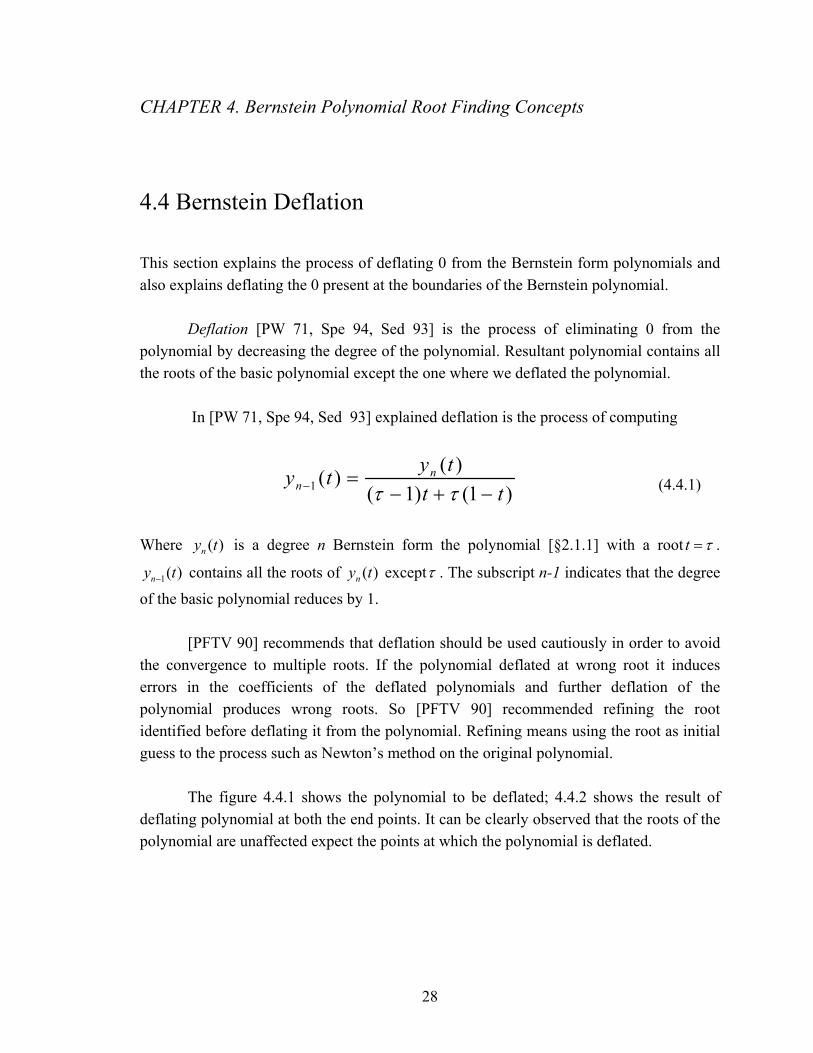
4.4 Bernstein Deflation

This section explains the process of deflating 0 from the Bernstein form polynomials and also explains deflating the 0 present at the boundaries of the Bernstein polynomial.

Deflation [PW 71, Spe 94, Sed 93] is the process of eliminating 0 from the polynomial by decreasing the degree of the polynomial. Resultant polynomial contains all the roots of the basic polynomial except the one where we deflated the polynomial. In [PW 71, Spe 94, Sed 93] explained deflation is the process of computing

1( )( )

( 1) (1n

ny ty ttτ τ− =

)t− + − (4.4.1)

Where is a degree n Bernstein form the polynomial [§2.1.1] with a root( )ny t t τ= .

contains all the roots of except1( )ny t− ( )ny t τ . The subscript n-1 indicates that the degree

of the basic polynomial reduces by 1.

[PFTV 90] recommends that deflation should be used cautiously in order to avoid the convergence to multiple roots. If the polynomial deflated at wrong root it induces errors in the coefficients of the deflated polynomials and further deflation of the polynomial produces wrong roots. So [PFTV 90] recommended refining the root identified before deflating it from the polynomial. Refining means using the root as initial guess to the process such as Newton’s method on the original polynomial.

The figure 4.4.1 shows the polynomial to be deflated; 4.4.2 shows the result of

deflating polynomial at both the end points. It can be clearly observed that the roots of the polynomial are unaffected expect the points at which the polynomial is deflated.

28


Figure 4.4.1. Polynomial to be deflated

Figure 4.4.2 Polynomial Deflated at both ends

29


4.5 Bernstein differentiation This section presents the Differentiation techniques for Bernstein polynomials. Some of the Bernstein Polynomial approximation techniques use differentiation to find the roots over a defined interval. One such algorithm is BCOM algorithm presented in [Spe 94]. Given a Bernstein form polynomial [§2.1.2]

( )[0,1]0

! (1 )! !

nn k k

kk

d ny y tdt k n k

−

=

⎛ ⎞= −⎜ ⎟⎜ ⎟−⎝ ⎠∑ t

where are coefficients and iy iε are corresponding errors for i =1, 2 ,…..n. Differentiation

results in a polynomial, whose coefficients are given as

for i=1, 2, …..n-1. 1(i i iy y y+′ = − ) nDifferentiation decreases the degree of polynomial by 1. It can be easily derived as follows

( )[ 0 ,1 ]0

! (1 )! !

nn k k

kk

d d ny y td t d t k n k

−

=

⎛ ⎞= ⎜ ⎟⎜ ⎟−⎝ ⎠∑ t− (4.5.1)

( ) ( ) ( )1 1! ( ) ! !(1 ) (1 ) (1 )

! ! ! ! ! !n k k n k k n k kd n n k n knt t t t t t

dt k n k k n k k n k− − −⎛ ⎞ ⎛ ⎞ ⎛ ⎞−

− = − + −⎜ ⎟ ⎜ ⎟ ⎜ ⎟⎜ ⎟ ⎜ ⎟ ⎜ ⎟− − −⎝ ⎠ ⎝ ⎠ ⎝ ⎠

− −

( ) ( )1 1( 1)! ( 1)!(1 ) (1 )

! 1 ! ! !n k k n k kn n n nt t t t

k n k k n k− − −⎛ ⎞ ⎛ ⎞− −

= − + −⎜ ⎟ ⎜ ⎟⎜ ⎟ ⎜ ⎟− − −⎝ ⎠ ⎝ ⎠

−

( ) ( )1 1

[0,1]0

( 1)! ( 1)!(1 ) (1 )! 1 ! ! !

nn k k n k k

k

d n n n ny yk t t t tdt k n k k n k

− − − −

=

⎛ ⎞⎛ ⎞ ⎛ ⎞− −= − −⎜ ⎟⎜ ⎟ ⎜ ⎟⎜ ⎟ ⎜ ⎟⎜ ⎟− − −⎝ ⎠ ⎝ ⎠⎝ ⎠∑ −

(4.5.2)

30

CHAPTER 4. Bernstein Polynomial Root Finding Concepts From the above equation we can easily derive

( )1

1[ 0 ,1]

0

( 1) !( 1 ) (1 )! 1 !

nn k k

k

d ny yk yk n td t k n k

−− −

=

⎛ ⎞−= + − −⎜ ⎟⎜ ⎟− −⎝ ⎠∑ t

iy

(4.5.3)

The accumulated error in the coefficients of the derivative polynomial, computed from the linearized error analysis, can be given by

12 | | ( )

ii i yy nε η ε ε+

′ ′= + + for i =1, 2, …n-1

The following figure illustrates the result of differentiating the Bernstein form polynomial.

Figure 4.5.1 Polynomial before Differentiation

31


Figure 4.5.2 Differentiated Bernstein form polynomial

Differentiation of polynomials is also useful for calculating the condition number of an approximated root [FR 87].

32

Chapter 5

Polynomial Approximation Algorithm

5.1 Bernstein Convex Hull Approximation Method Bernstein convex hull approximation method uses the convex hull property, all the roots of a polynomial lie in the interval where the control polygon intersects the abscissa, of the Bèzier curves to approximate the real roots of a Bernstein form polynomial. This algorithm was first appeared in [Gra89, sch90a]. Actually this algorithm was first overviewed in [sp86], fully discussed in [ssd86]. The algorithm approximates all the real roots of the polynomial in ascending order over the interval [0, 1] using a sequence of approximation steps, which are guaranteed to not skip over a root. Root is realized when the approximation steps converge to a limit.

This section present similar kind of algorithm which uses convex hull property to approximate all the real roots of the polynomial in ascending order over the interval [0,1]. This algorithm uses the concepts described in the section 4.

Section [§5.1.1] explains the process of computing the approximation step for

approximation of real roots of Bernstein form polynomial. Section [§5.1.2] explains the steps in Bernstein Convex Hull algorithm and explains the process with the help of example. Section [5.1.3] explains the modifications made to the above discussed algorithm to improve the precision and to find the multiplicity of the root.

33

CHAPTER 5. Polynomial Approximation Algorithm 5.1.1 Approximation step This section describes the process of computing approximation step, which are used to approximate the real roots of Bernstein form polynomial. Two of such techniques, 1BCHA , 2 4BCHA − 1BCHA [thesis], are presented here. 1BCHA finds the most

positive slope of the curve based upon the left most intersection of the control polygon with the t-axis. 2 4BCHA − is variant of 1BCHA , which provides greater convergence.

1BCHA Approximation step This method finds the steepest slope of the curve based upon the left most intersection of the convex hull with the t-axis. This is similar to the Newton’s step but the advantage is it approaches the root from the left, unlike the Newton’s method which diverges. This method uses a split heuristic to speed up the process of approaching a root. Here we explain the method using the following example.

Consider a Bernstein form polynomial expressed in the form of explicit Bèzier curve, whose control points are [8,-6,-22, 40, 8,-9] (degree 5 polynomial). Plot of the curve over interval [0, 1] is given in fig 5.1.1.

The approximation step for this curve is calculated by computing the maximum

slope of absolute slopes of all the lines joining the first control point to the other control points. Let denote the absolute slope of the line joining the first control point to control point

for i=2,…n. So is i

1

2

3

6 8 5 70

22 8 5 752

40 8 16053 3

s

s

s

= − − × =

− −= × =

−= × =

34

CHAPTER 5. Polynomial Approximation Algorithm

Figure 5.1.1 Bernstein polynomial

4

5

8 8 5 049 8 5 175

s

s

−= × =

− −= × =

35


2s is the maximum absolute slope of all the lines. The intersection of the control polygon

with the t-axis is computed using 1

2

yts

= − where is y-coordinate of first control point,

is the maximum absolute slope we obtained above. Therefore the approximation step is

1y

2s

( 8) .106775

t −= − =

It is evident from the above figure [§5.1.1] that the obtained value is true and it makes good initial approximation of the root.

BCHA2-4 Approximation Step: An improvement of BCHA1 approximation step was discussed in [Sep 94]. This approximation step gives higher order convergence. This algorithm makes use of the closed form root solving algorithms of polynomials in power basis.

The basic idea behind this is approach is to device approximating polynomials of degree two, three and four whose left most root are guaranteed to be less than the left most root of the master polynomial. Once the left most root of such polynomial is obtained it is used as step for isolating the root of master polynomial. We can easily find the root of such approximated polynomials using closed form root solvers [Spe 94].

This degree two, three and four polynomials can be easily approximated from the explicit Bezier curve representation. [Spe 94] discusses this method in greater detail.

5.1.2 BCH Algorithm This section presents the main algorithm steps and presents the Matlab code for approximating the roots of the polynomial in Bernstein form.

36

CHAPTER 5. Polynomial Approximation Algorithm Pre-approximation steps

1. Read the coefficients {Y} of the polynomial (master polynomial) and the initial errors in the coefficients of the polynomial in which we are interested.

2. Normalize the coefficients and errors to prevent the overflow and underflow in

floating-point arithmetic using [§4.1].

3. Test for the rightmost root (s) of the polynomial, i.e. at the upper limit of the interval [0, 1].

4. Test for the leftmost root(s) of the polynomial, i.e. at the lower limit of the interval

[0, 1] and record the roots.

5. Initialize the left {Yl} and right{Yr} sub polynomials and assign them to the master polynomial over the same interval as the master polynomial. Left sub polynomial is the active polynomial, right sub polynomial is used to keep track of the remaining polynomial (polynomial that is to be approximated).

6. Initialize the rootfound flag to 0. Zero (0) value of the flag indicates root not found

and one(1) value of the flag indicates root is found. Real Root Approximation steps

1. Test for the root, check if the rootfound=1 then record the root, subdivide the right{Yr} sub polynomial at the root, returning the right subdivided polynomial as new right sub polynomial. Assign the right sub polynomial {Yr} to the left sub polynomial {Yl}, deflate the root and proceed to step 2. If rootfound=0 proceed to step 2.

2. Test if the control polygon straddles the t-axis. This can be done by checking the

sign variations in the coefficients of the polynomial. If there is at least a sign

37


change there can at least be one root. If there are no sign changes there is no root (Descrete’s rule of signs). 3. If there are sign changes

3.1 compute the approximation step (t) using one of the methods described in [§5.1.1]

3.2 Store the left subdivided polynomial {Yl} as temporary {Yt1} segment. This

is useful if the approximation step overshoots the root.

3.3 Subdivide the left sub polynomial {Yl} at t, returning the right subdivided polynomial as new left sub polynomial and the left subdivided polynomial as 2nd temporary polynomial {Yt2}.

3.4 Test for the convergence, if convergence satisfied set rootfound flag to 1 and

go to step 1.

3.5 Test for the overshooting root, if we overshoot the root check split flag. If split=0 then assign the stored first temporary segment {Yt1} to the left sub polynomial {Yl} and proceed to step1. If split is not equal to 0 test for the convergence of root and refine the root using regular-falsi method, proceed to step 1.

3.6 If split=1 then subdivide the left sub polynomial at t= first sign changing

coefficient/degree, returning the left subdivided polynomial as new left sub polynomial and proceed to step 1.

4. If there are no sign changes then no root exists in the active polynomial. If the

upper limit of left sub polynomial is not equal to the upper limit of right sub polynomial sub divide the right sub polynomial {Yr} at upper limit of left sub polynomial returning the right subdivided polynomial as new left and right sub polynomials, proceed to step 1.

38

CHAPTER 5. Polynomial Approximation Algorithms 5. Record the right most root found at step 3 of pre-approximation step and return

all the roots. The figure 5.1.2 illustrates the process of approximating roots using the Bernstein Convex Hull approximation algorithm. At each step approximation step is calculated using one of the methods specified in 5.1.1. The progression is stopped when the approximation step converges to a limit as shown in 4.4.2(d) The approximation step never overshot a root because of the convex hull property, but numerically the computational errors induced by round-off may allow the step to overshoot. BCH algorithm that uses BCHA1 approximation step has a disadvantage in the form of requiring de Casteljau algorithm at each step, whose complexity is O(n2), even though it has an advantage of never overshooting a root, where as the BCH algorithm that uses BCHA2-4 approximation step is faster than the first one.

5.1.3 Modified BCH Algorithm This section presents the modified form of the above discussed algorithm. Two changes were made to the above algorithm to increase the precision of the root and to find the multiplicity of the root. Once the root is found in the step 3.4 of [5.1.2] it is refined using Newton’s method and the root is checked for multiplicity. Multiplicity of a root is obtained by evaluating the differential polynomial (obtained by differentiating the basic polynomial) at the root, if it is root multiplicity of the root is two. Then the second derivative of the polynomial is evaluated at the root, if its value is zero multiplicity of the root is 3. The process is repeated until nth differential polynomial’s evaluated at the root and the multiplicity of the root is n+1. If the evaluated value is not zero or greater than the error the program stops for checking multiplicity and proceeds to find the next root.

39


Figure 5.1.2. BCH Root finding

40

Chapter 6

Numerical Results and Discussion This chapter presents results of empirical testing carried out on the BCHA algorithm discussed in section [§5.1.3]. The algorithms are tested in Double precision arithmetic on P-IV machine with round-off unit 1.1102230246251565E-16. The algorithm is tested over some of the polynomials presented in [Zen] and results are discussed below. All the polynomial presented here are converted into power basis using the POLY function of MATLAB.

Jenkins-Traub’s test polynomials Degree 8 polynomial

( .1) ( .0 1) ( .0 0 1) . . .( .0 0 0 0 0 0 0 1)x x x x− − − − Numerical results of approximating algorithm are compared with the actual results in table 6.1

ROOT NUMBER

ACTUAL ROOTS

MULTI- PLICITY

APPROXIMATED ROOTS

MULTI- PLICITY

1 0.00000001 1 0.00000001000000 1 2 0.0000001 1 0.00000010000000 1 3 0.000001 1 0.00000100000000 1 4 0.00001 1 0.00001000000000 1 5 0.0001 1 0.00010000000000 1 6 0.001 1 0.00100000000000 1 7 0.01 1 0.00999999999999 1 8 0.1 1 0.01000000000000 1

Table 6.1 Degree 8 Polynomial

41

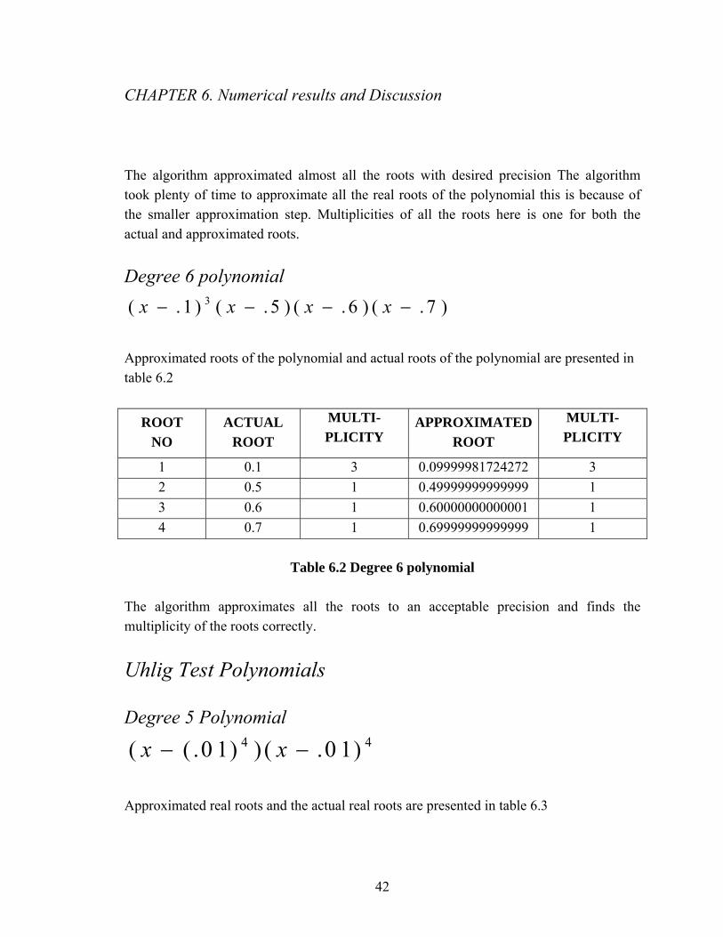
CHAPTER 6. Numerical results and Discussion The algorithm approximated almost all the roots with desired precision The algorithm took plenty of time to approximate all the real roots of the polynomial this is because of the smaller approximation step. Multiplicities of all the roots here is one for both the actual and approximated roots.

Degree 6 polynomial 3( . 1 ) ( . 5 ) ( . 6 ) ( . 7x x x x− − − − )

Approximated roots of the polynomial and actual roots of the polynomial are presented in table 6.2

ROOT NO

ACTUAL ROOT

MULTI- PLICITY

APPROXIMATED ROOT

MULTI- PLICITY

1 0.1 3 0.09999981724272 3 2 0.5 1 0.49999999999999 1 3 0.6 1 0.60000000000001 1 4 0.7 1 0.69999999999999 1

Table 6.2 Degree 6 polynomial

The algorithm approximates all the roots to an acceptable precision and finds the multiplicity of the roots correctly.

Uhlig Test Polynomials

Degree 5 Polynomial 4 4( ( .0 1) ) ( .0 1)x x− −

Approximated real roots and the actual real roots are presented in table 6.3

42

CHAPTER 6. Numerical results and Discussion

ROOT NO

ACTUAL ROOT

MULTI- PLICITY

APPROXIMATED ROOT

MULTI- PLICITY

1 0.00000001 1 0.00000001000000

3

2 0.01 4 0.00999800469919 0.01000112701649

4 4

Table 6.3 Degree 5 polynomial

For this polynomial no of roots approximated were 3 but the actual number of roots were2. The algorithm failed to approximate the roots to the precision and failed to approximate the multiplicity correctly as well. This is also due the errors induced during the conversion of polynomial in [App3] to Bernstein form.

Igarashi-Ypma Test Polynomials

Degree 3 Polynomial ( .35)( .37)( .39)x x x− − − Resultant roots of the algorithm and their multiplicities are compared in the table 6.4

ROOT NO

ACTUAL ROOT

MULTI- PLICITY

APPROXIMATED ROOT

MULTI- PLICITY

1 0.35 1 0.34999999999998 1

2 0.37 1 0.37000000000002 1

3 0.39 1 0.38999999999998 1


43

CHAPTER 6. Numerical Results and Discussion

The algorithm approximated the roots and multiplicity correctly for this kind of polynomials.

Degree 4 Polynomial 3( . 3 5 ) ( . 5 6 )x x− −

Roots approximated using the algorithm and their multiplicities are presented in table 6.4

ROOT NO

ACTUAL ROOT

MULTI- PLICITY

APPROXIMATED ROOT

MULTI- PLICITY

1 0.35 3 0.35001314222638 3

2 0.56 1 0.55999999999999 1


The algorithm approximated the roots to the satisfactory precision and computed the multiplicities correctly for all the roots. The errors in the roots are due to the conversion errors induced in the coefficients of Bernstein polynomial while converting the [App 5] polynomial to Bernstein form.

Zeng Test Polynomials Degree 16 Polynomial

8 8( . 3 9 ) ( . 4 )x x− − Approximated real roots and their multiplicities are compared with the actual roots and their multiplicities in table 6.5

44

CHAPTER 6. Numerical Results and Discussion

ROOT NO

ACTUAL ROOT

MULTIPL- ICITY

APPROXIMATED ROOT

MULTIPL- CITY

1 0.39 8 0.34408056556175 8

2 0.4 8 0.47195807132900 7

Table 6.5Degree 16 polynomial

The algorithm produced results are not satisfactory. This is due to the error in the initial coefficients of the Bernstein form polynomial.

Degree 30 polynomial with Bernstein Coefficients [8,9,10,-22,-10,-8,-2,10,12,4.8976786,8.5678,-1.3435,-6,-7,-1,0,27,8,7,6.4546,11,-9,-33,.56789,-12,-23,10,11,2.3456,10] Roots and multiplicities of the polynomial approximated from the algorithm [5] are

ROOT NO

APPROXIMATED ROOT

MULTIPL- CITY

1 0.07474873932098 1

2 0.21854143583840 1

3 0.67893594400194 1

4 0.89849858009515 1

The algorithm approximated all the roots of this polynomial satisfactorily.

45

Conclusions & Future Work This Dissertation addresses the well known problem of Approximating real roots of a polynomial in Bernstein form over a finite interval, which has greater application in Computer-Aided Graphics Design. The importance of Bernstein form polynomials to CAGD comes from the extensive use of Bezier curves and numerical stability of the Bernstein basis.

The thesis discusses the explicit representation of Bezier curves in the form of Bernstein form polynomials and also the properties that are useful for the approximation of real roots. The thesis also discusses the numerical conditions of Bernstein form polynomials including forward error analysis, preconditioning and backward error analysis in floating-point arithmetic.

Many algorithms have been proposed over years to approximate the real roots of the Bernstein form polynomial over a finite interval. The thesis describes some of these methods in brief. The dissertation not proposes any new method to approximate the real roots of Bernstein form polynomial. It implements the Bernstein Convex Hull Approximation method proposed by Melvin. R. Spencer and tries to improve it.

The BCH Algorithm have been modified to improve the accuracy of the roots and to find the multiplicity of the roots. Here Newton’s method has been used to improve the accuracy of the root, taking the root found in BCH algorithm as the initial guess for Newton’s method. Multiplicity of the root if found by evaluating the first, second,.. , nth derivatives at the root found.

The algorithm approximates all the real roots of a Bernstein form polynomial to satisfactory precision and multiplicities in reasonable amount of time. But the algorithm failed to approximate all the real roots of a Bernstein polynomial with clustered roots. One such polynomial is presented in chapter [6]. This is due to the very small approximation step (which is necessary for approximating clustered roots). The algorithm also failed in some cases to approximate the multiplicities correctly for a polynomial, whose roots are of multiplicity more than 8. The algorithm works fine for most of the polynomials. Future work on this algorithm can be done to improved to approximate the roots more accurately and the multiplicities correctly for any degree polynomial.

46

BIBLIOGRAPHY

[Ber12] Bernstein, S.N. (in Russian), On the best approximation of continuous functions by a polynomial of given degree. Comm.Kharkow Math. Soc., series 2, 13: 49-194, 1912. [BFK 84] Wolggang Bohm, Gerald Frain and Jurgen Kahmann. A survey of curve and surface methods in cagd. Computer Aided Geometric Design, 1: 1-60, 1984. [Dun 72] Donna K.Dunway, A Composite Algorithm for Finding Zeros of a Real Polynomilas. PhD thesis, Southern Methodist University, August 21 1972. FORTRAN code included. [Far 86] R.T. Farouki. The characterization of parametric surface sections.Comp- uter Vision, Graphics, and Image Processing, 33:209-236, 1986. [FJ 94] R.T. Farouki and Johnstone. The bisector of a plane parametric curve Computer Aided Geometric Design 11, 1994 [FR 87] R.T. Farouki and V.T. Rajan. On the numerical conditions of polynomials in Bernstein form. Computer Aided geometric Design, 4:191-216, 1987. [FR 88] R.T. Farouki and V.T. Rajan. Algorithms for polynomials in Bernstein form. Computer Aided Geometric Design, 5:1-26, 1988. [Fra 84] G.Frain. Survey of Curve and Surface Methods in CAGD, Computer Aid- ed Graphics Design,1:1-60,1984. [GRA 89] Thomas A. Grandine. Computing zeros of spline functions. Computer Ai- ded Geometric Design, 6:129-136, 1989.

47

BIBLIOGRAPHY [JEN 75] M.A. Jenkins Algorithm 493: Zeros of a real polynomial [c2]. ACM Transaction on Mathematical Software, 1(2): 178-192, June 1975. [LR 81] Jeffrey M. Lane and Richard F. Riesenfeld. Bounds on a polynomial BIT, 21:112-117, 1981. [MC 90] Denis marchepoil and Patric Chenin. Algorithmes de recherché de zéros dún fonction de Bézier. Laboratoire de Modélosation et Calcul RR 843-I & M-, Institut National Polytechnique de Grenoble Université Joseph Fourier Grenoble 1, Centre National de la Recherche Scintifique, Ecole Mormale Supérieure do Lyon, November 1990. [Ost 54] Ostrowski A. On two problems in abstract algebra connected with Horner’s rule, Studies in Mathematics and Mechanics presented to R. von Mises , Ac- ademic press, New York, 40-48, 1954. [Pav 82] Theo Pavlidis. Algorithms for Graphics and Image Processing. Computer S- cience press, Rockville, MD, 1982. [PFTV 90] William H. Press, Brian P. Flannery, Saul A. Teukolsky, and William T. Vetterling. Numerical Recipes in C: The Art of Scientific Computing. Cam- Bridge University Press, Cambridge, 1990. [PW 71] G. Peters and J.H. Wilkinson. Practical problems arising in the solutions of polynomial equations. J. Inst. Maths Applies, 8: 16-35, 1971.

48

BIBLIOGRAPHY [Roc 89] Alyn Rockwood. Constant component intersections of parametrically defined curves. Technical report, Silicon Graphics Computer Systems, 1989. [Sch 90a] Philip J, Schneider. A Bézier curve based root finder. In Andrew S. Glass- ner, editor, Graphics Gems, pages 408-415, 787-797. Academic Press, Inc., San Diego, CA, 1990. C code included. [Sed 85] Thomas W. Sederberg. Piecewise algebraic surface patches. Computer-Aided Geometric Design, 2:53-59, 1985. [SP 86] Thomas W. Sederberg and Scott R. Parry. Comparision of three Curve Inter- section Algorithms, Computer-aided geometric Design, 18(1):58-63, January /February 1986. [SSd 86] Thomas W. Sederberg, Melvin R. Spencer, and Carl de Boor. Real Root Ap- proximation of polynomial in Bernstein form. Draft copy, December 1986. [Spe 94] Melvin R. Spencer. Polynomial Real Root Finding in Bernstein Form, A Diss- ertation presented to the Department of Civil Engineering, Brigham Young University, August 1994. [WIL 60] J.H. Wilkinson. Error Analysis of Floating-point Computation, Numer, Math, 2:319-340, 1960. [Zen] Zhonggang Zeng. MULTROOT- A Matlab Package Computing polynomial roots and their Multiplicities(http://www.neiu.edu/~zzeng/Papers/zrootpak.pdf).

49

a bernstein polynomail root solver

Documents