A Beginner’s Guide to Matrix Algebra &Matrix Linear Regression Using Stata (Mata)

Jason Eichorst, Rice Universityjaeichorst@rice.edu

Poli 503

September 8, 2009

Abstract

This guide is intended for an audience that understand the basics of Stata (if not,read A Beginner’s Guide to Using Stata and has an introductory understanding ofmatrix algebra and the matrix approach to the linear regression model. I show thereader how to use Stata (more specifically, Mata) to perform matrix algebra and thematrix linear regression model. This guide is produced while using Stata Version 10on a Mac.

1 Introduction

I assume that the reader has some basic knowledge using Stata and has an introductoryunderstanding of matrix algebra and the matrix linear regression model. Gujarati (2003)provides an excellent introduction to matrix algebra and the matrix linear regression modelin Appendix B & C for those readers without this introductory understanding.

The user will be instructed in Stata using Mata. Although there are two different methodsfor performing matrix algebra in Stata, I choose Mata because it efficiently manages data setsand allows the user to perform interactive matrix calculations. This guide only touches thesurface of Mata, more advanced users can use Mata for programming and many more matrixapplications. I also briefly introduce matrix algebra using Stata. My principle resources fordeveloping this guide are the [M] Mata manual and Gujarati (2003). The reader can alsoreceive Mata help through Stata by typing help mata in the command line or receive helpusing matrices in Stata by typing help matrix in the command line. An additional resourceincludes: http://ideas.repec.org/p/boc/dsug09/06.html. Finally, don’t forget to startyour log-file and use a do-file while practicing these commands.

1

1.1 Mata

Mata is a matrix programming language that can be used to perform matrix calculationsinteractively, perform interact functions, and can be used by those who want to add newfeatures to Stata. Mata is new to Stata, recently included with Version 9 (2005). Mataavoids many of the limitations of Stata’s traditional matrix commands. Mata creates virtualmatrices, or views, that refer directly to Stata variables and requires very little memoryusage. This is unlike matrices created using traditional Stata commands that consume asignificant amount of memory to produce a matrix and are limited to 800 rows or columnin Intercooled Stata. Further, Mata can be efficiently used for programming. The user mustenter mata to start the Mata session and enter end to return to Stata. The user can start andend Mata throughout an entire session without losing memory stored in Mata, this makes itpossible to transition out of Mata to use commands in Stata and vice versa. To clear Mata’smemory, type mata clear. The Mata prompt is indicated using colons, :, unlike in Stata,which uses periods, ..

. clear mata

. mata--------------------------------- mata (type end to exit) -------------------: 2 + 24

:: 2 + 1i + 3i + 57 + 4i

: end-----------------------------------------------------------------------------

. clear

1.2 Creating Matrices

Creating a Matrix in Mata is relatively simple, the user is only required to learn two ad-ditional operators: 1) ‘,’ is the column-join operator and 2) ‘\’ is the row-join operator.Although parentheses are often times unnecessary when creating matrices, users often in-clude them in their commands for presentational purposes in their code. Note: if you arehave any problems creating these matrices or running the commands, then make sure youare in the Mata prompt and not in the Stata prompt (i.e. look for the semi-colons).

1.2.1 String Matrix

Let’s create this string matrix

[a bc d

]in Mata.

2

: ("a","b"\"c","d")1 2

+---------+1 | a b |2 | c d |

+---------+

1.2.2 Numeric Matrix

Let’s do the same for this numeric matrix

[1 23 4

].

: (1,2\3,4)1 2

+---------+1 | 1 2 |2 | 3 4 |

+---------+

Let’s use Mata to create a more complex matrix,

4 5 7 923 10 9 552 7 92 2143 89 1 305 33 7 9

.

: (4,5,7,9)\(23,10,9,55)\(2,7,92,21)\(43,89,1,30)\(5,33,7,9)1 2 3 4

+---------------------+1 | 4 5 7 9 |2 | 23 10 9 55 |3 | 2 7 92 21 |4 | 43 89 1 30 |5 | 5 33 7 9 |

+---------------------+

1.2.3 Scalar

Create a scalar, which is just a 1x1 matrix.

: s=2

: s2

1.2.4 Row Vector

Creating a row vector requires only using the column-join operator, ‘,’.

3

: X = (3,5,9)

: X1 2 3

+-------------+1 | 3 5 9 |

+-------------+

The user can create a row vector of sequential numbers using ‘..’. For example,[1 2 3 4

]can be created using (1..4).

: Y = (1..3)

: Y1 2 3

+-------------+1 | 1 2 3 |

+-------------+

1.2.5 Column Vector

Creating a column vector requires only using the row-join operator, \.

: A = (2\4\7\3\6)

: A1

+-----+1 | 2 |2 | 4 |3 | 7 |4 | 3 |

+-----+

The user can create a column vector of sequential numbers using ‘::’. For example,

1234

can

be created using (1::4).

: B = (1::4)

: B1

+-----+1 | 1 |2 | 2 |3 | 3 |4 | 4 |

4

+-----+

1.2.6 Combine Matrices

Users are able to combine already defined matrices to create a larger matrix. This can beseen as a shortcut, instead of rewriting the elements of a matrix to produce a larger matrix.Using parentheses, even if excessive, help visualize the construction of the matrix. In thisexample, I will use row vectors X & Y and column vector B to create a 4x4 matrix calledG.

: G = (X\Y\(4,5,2)\(10..8)),B

: G1 2 3 4

+---------------------+1 | 3 5 9 1 |2 | 1 2 3 2 |3 | 4 5 2 3 |4 | 10 9 8 4 |

+---------------------+

1.2.7 uniform()

uniform() pulls random draws from uniform[0,1] to fill elements in a matrix. The userdefines the dimension of the matrix in the parentheses. This is a quick way to randomly filla matrix with numbers between 0 and 1. Here, I create a 3x4 matrix called H.

: H = uniform(3,4)

: H1 2 3 4

+---------------------------------------------------------+1 | .7517702221 .742742738 .7448844064 .4513101887 |2 | .1536625174 .0538137804 .7708901914 .5452894035 |3 | .4481307138 .2635594367 .7811205103 .0333320007 |

+---------------------------------------------------------+

1.2.8 invnormal(uniform())

invnormal(uniform()) pulls random draws from a standard normal distribution to fillelements in a matrix. Just like above, the user defines the dimension of the matrix inthe parentheses. This, too, is a quick way to fill a matrix. Here, I create a 4x4 matrix calledJ.

: J = invnormal(uniform(4,4))

5

: J1 2 3 4

+-------------------------------------------------------------+1 | -1.042549855 -1.917328014 -.7675750582 .5456267302 |2 | .6060552032 .1862779936 1.302701542 -.8391142665 |3 | -.4616685313 1.20684494 1.02573929 -.2559725192 |4 | 1.276908608 -.1891663191 -.2918787981 1.300406279 |

+-------------------------------------------------------------+

1.2.9 Transposition

The nice aspect about Mata is that it follows writing convention. Transpose is indicatedusing an apostrophe, ’.

: X1 2 3

+-------------+1 | 3 5 9 |

+-------------+

: X’1

+-----+1 | 3 |2 | 5 |3 | 9 |

+-----+

: G1 2 3 4

+---------------------+1 | 3 5 9 1 |2 | 1 2 3 2 |3 | 4 5 2 3 |4 | 10 9 8 4 |

+---------------------+

: G’1 2 3 4

+---------------------+1 | 3 1 4 10 |2 | 5 2 5 9 |3 | 9 3 2 8 |4 | 1 2 3 4 |

+---------------------+

6

: G’’1 2 3 4

+---------------------+1 | 3 5 9 1 |2 | 1 2 3 2 |3 | 4 5 2 3 |4 | 10 9 8 4 |

+---------------------+

1.2.10 Submatrix

Elements and submatrices can easily be created using Mata. Notice the use of brackets, [and ], to call elements and create submatrices. In this example, I create different partitionsfrom the G matrix.

Call an element using brackets.

: G[3,2]5

Place a period, ‘.’, in the column option to return the entire row.

: G[2,.]1 2 3 4

+-----------------+1 | 1 2 3 2 |

+-----------------+

Place a period, ‘.’, in the row option to return the entire column.

: G[.,2]1

+-----+1 | 5 |2 | 2 |3 | 5 |4 | 9 |

+-----+

Specify elements to create a submatrix.

: G[|2,1\3,4|]1 2 3 4

+-----------------+1 | 1 2 3 2 |2 | 4 5 2 3 |

+-----------------+

Specify rows and columns to recreate the same submatrix from above.

: G[(2::3),(1..4)]

7

1 2 3 4+-----------------+

1 | 1 2 3 2 |2 | 4 5 2 3 |

+-----------------+

1.3 Types of Matrices

There are a variety of different types of matrices. I show how some of these matrices can becreated using Mata. This list of examples and processes is not exhaustive.

1.3.1 Matrix of Constants

J() takes three arguments to create a matrix of constants. The first two arguments identifythe dimension of the matrix and the third argument identifies the constant.

: J(4,3,5)1 2 3

+-------------+1 | 5 5 5 |2 | 5 5 5 |3 | 5 5 5 |4 | 5 5 5 |

+-------------+

1.3.2 Null Matrix

Use J() to create a null matrix.

: J(4,4,0)[symmetric]

1 2 3 4+-----------------+

1 | 0 |2 | 0 0 |3 | 0 0 0 |4 | 0 0 0 0 |

+-----------------+

1.3.3 Unit Matrix

Use J() to create a unit matrix

8

: J(3,2,1)1 2

+---------+1 | 1 1 |2 | 1 1 |3 | 1 1 |

+---------+

1.3.4 Identity Matrix

I() takes one argument that identifies the length of the diagonal to create an identitymatrix.

: I(4)[symmetric]

1 2 3 4+-----------------+

1 | 1 |2 | 0 1 |3 | 0 0 1 |4 | 0 0 0 1 |

+-----------------+

1.3.5 Scalar Matrix

Multiple an identity matrix by a scalar to create a scalar matrix.

: 8*I(4)[symmetric]

1 2 3 4+-----------------+

1 | 8 |2 | 0 8 |3 | 0 0 8 |4 | 0 0 0 8 |

+-----------------+

1.3.6 Diagonal Matrix

diag() can create a diagonal matrix from an already defined matrix, or it can create adiagonal when it is given elements.

Create a diagonal matrix from G.

: diag(G)[symmetric]

9

1 2 3 4+-----------------+

1 | 3 |2 | 0 2 |3 | 0 0 2 |4 | 0 0 0 4 |

+-----------------+

Create a diagonal matrix using elements.

: diag((3,4,2,5))[symmetric]

1 2 3 4+-----------------+

1 | 3 |2 | 0 4 |3 | 0 0 2 |4 | 0 0 0 5 |

+-----------------+

1.3.7 Extract Diagonal into Column Matrix

diagonal() extracts a diagonal to create a column matrix.

: diagonal(G)1

+-----+1 | 3 |2 | 2 |3 | 2 |4 | 4 |

+-----+

1.3.8 Symmetric Matrix

A symmetric matrix is such when the transpose equals itself.

: K=1,3,5\3,7,4\5,4,9

: K[symmetric]

1 2 3+-------------+

1 | 1 |2 | 3 7 |3 | 5 4 9 |

+-------------+

10

: K’[symmetric]

1 2 3+-------------+

1 | 1 |2 | 3 7 |3 | 5 4 9 |

+-------------+

2 Matrix Algebra

2.1 Addition

To perform addition, matrices must have the same dimensions.

: G+J1 2 3 4

+---------------------------------------------------------+1 | 2.808726649 6.272184186 9.054984923 2.000267399 |2 | .1970702137 2.162157713 2.371389651 3.623349516 |3 | 3.407970481 3.81503605 1.767230638 3.588641675 |4 | 11.13442122 8.90244514 7.802383661 5.250681085 |

+---------------------------------------------------------+

: J+G1 2 3 4

+---------------------------------------------------------+1 | 2.808726649 6.272184186 9.054984923 2.000267399 |2 | .1970702137 2.162157713 2.371389651 3.623349516 |3 | 3.407970481 3.81503605 1.767230638 3.588641675 |4 | 11.13442122 8.90244514 7.802383661 5.250681085 |

+---------------------------------------------------------+

2.2 Subtraction

To perform subtraction, matrices must have the same dimensions.

: G-J1 2 3 4

+---------------------------------------------------------+1 | 3.191273351 3.727815814 8.945015077 -.000267399 |2 | 1.802929786 1.837842287 3.628610349 .3766504841 |3 | 4.592029519 6.18496395 2.232769362 2.411358325 |4 | 8.865578777 9.09755486 8.197616339 2.749318915 |

11

+---------------------------------------------------------+

: J-G1 2 3 4

+-------------------------------------------------------------+1 | -3.191273351 -3.727815814 -8.945015077 .000267399 |2 | -1.802929786 -1.837842287 -3.628610349 -.3766504841 |3 | -4.592029519 -6.18496395 -2.232769362 -2.411358325 |4 | -8.865578777 -9.09755486 -8.197616339 -2.749318915 |

+-------------------------------------------------------------+

Let’s see what happens when the dimensions are different.

: H-J<istmt>: 3200 conformability error

r(3200);

2.3 Scalar Multiplication

Each element is multiplied by the scalar.

: 5*G1 2 3 4

+---------------------+1 | 15 25 45 5 |2 | 5 10 15 10 |3 | 20 25 10 15 |4 | 50 45 40 20 |

+---------------------+

2.4 Matrix Multiplication

Matrices must be conformable following the row by column rule of multiplication. Forexample, matrix ( MxN) is conformable to matrix ( NxM).

: G*J1 2 3 4

+-------------------------------------------------------------+1 | -8.782313433 -6.134889286 -5.270637572 17.66600593 |2 | -1.304379035 -2.153501958 -2.295776538 8.514253625 |3 | -2.560537704 3.236932827 -3.981499791 17.04714378 |4 | -9.337652845 4.311330236 -7.760264157 34.32467737 |

+-------------------------------------------------------------+

: J*G1 2 3 4

+-------------------------------------------------------------+

12

1 | 10.92097782 10.86533283 10.20720144 6.519119388 |2 | 11.47242212 7.776760393 4.989680491 4.128952656 |3 | 1.99428679 -1.196147235 -4.639562849 -1.305698807 |4 | 15.02205431 15.74504447 19.52734243 5.349186827 |

+-------------------------------------------------------------+

: H*G1 2 3 4

+---------------------------------------------------------+1 | 9.333329118 10.20352469 9.116481648 5.516010273 |2 | 5.245666218 7.280080464 8.209014138 3.001141384 |3 | 4.002953098 6.195510912 8.477946868 3.241661827 |

+---------------------------------------------------------+

Here’s what happens in Stata when matrices are non-conformable.

: G*H*: 3200 conformability error

<istmt>: - function returned errorr(3200);

Mata makes it easy to multiply elements.

: H[1,1]*G[1,2].6849203922

A row vector postmultiplied by a column vector is a scalar.

: (1..4)*(9::6)70

A column vector postmultiplied by a row vector is a matrix.

: (9::6)*(1..4)1 2 3 4

+---------------------+1 | 9 18 27 36 |2 | 8 16 24 32 |3 | 7 14 21 28 |4 | 6 12 18 24 |

+---------------------+

A matrix postmultiplied by a column vector is a column vector.

: G*A1

+-------+1 | 92 |2 | 37 |3 | 51 |4 | 124 |

+-------+

13

A row vector postmultiplied by a matrix is a row vector.

: (1..4)*G1 2 3 4

+---------------------+1 | 57 60 53 30 |

+---------------------+

2.5 Determinant

Every square matrix has a determinant that corresponds to a single number.

: det(G)-170

: det(K)-89

2.6 (Square) Matrix Inversion

The inverse of a square matrix can be found using the formula, A−1 = 1|A|(adjA). This

requires finding the determinant of the matrix, replacing each element by its cofactor toobtain the cofactor matrix, transposing the cofactor matrix to obtain the adjoint matrix,and dividing each element of the adjoint matrix by the determinant of the original matrix.In Mata, this can be accomplished using luinv().

: luinv(G)1 2 3 4

+-------------------------------------------------------------+1 | -.1941176471 .0294117647 -.3470588235 .2941176471 |2 | .2941176471 -.5294117647 .6470588235 -.2941176471 |3 | .0411764706 .2058823529 -.2294117647 .0588235294 |4 | -.2588235294 .7058823529 -.1294117647 .0588235294 |

+-------------------------------------------------------------+

: luinv(K)1 2 3

+----------------------------------------------+1 | -.5280898876 .0786516854 .2584269663 |2 | .0786516854 .1797752809 -.1235955056 |3 | .2584269663 -.1235955056 .0224719101 |

+----------------------------------------------+

For fun, let’s explore some of the properties of inverted matrices.

(AB)−1 = B−1A−1

14

: luinv(G*J)1 2 3 4

+-------------------------------------------------------------+1 | 3.670259918 -6.400568483 4.920867244 -2.523139126 |2 | -3.69316525 6.343976868 -5.365095557 2.797659096 |3 | 2.552541249 -4.66571623 3.91014391 -1.967404133 |4 | 5.230244908 -8.959482404 7.022434919 -3.587841537 |

+-------------------------------------------------------------+

: luinv(J) * luinv(G)1 2 3 4

+-------------------------------------------------------------+1 | 3.670259918 -6.400568483 4.920867244 -2.523139126 |2 | -3.69316525 6.343976868 -5.365095557 2.797659096 |3 | 2.552541249 -4.66571623 3.91014391 -1.967404133 |4 | 5.230244908 -8.959482404 7.022434919 -3.587841537 |

+-------------------------------------------------------------+

(A−1)′ = (B−1)′

: luinv(G)’1 2 3 4

+-------------------------------------------------------------+1 | -.1941176471 .2941176471 .0411764706 -.2588235294 |2 | .0294117647 -.5294117647 .2058823529 .7058823529 |3 | -.3470588235 .6470588235 -.2294117647 -.1294117647 |4 | .2941176471 -.2941176471 .0588235294 .0588235294 |+-------------------------------------------------------------+

: luinv(G’)1 2 3 4

+-------------------------------------------------------------+1 | -.1941176471 .2941176471 .0411764706 -.2588235294 |2 | .0294117647 -.5294117647 .2058823529 .7058823529 |3 | -.3470588235 .6470588235 -.2294117647 -.1294117647 |4 | .2941176471 -.2941176471 .0588235294 .0588235294 |+-------------------------------------------------------------+

AA−1 = A−1A = I

Note: Off-diagonals are not exactly zero, but near, because of rounding error during Mata’scalculation.

: G*luinv(G)1 2 3 4

+-------------------------------------------------------------+1 | 1 1.11022e-16 6.10623e-16 -2.63678e-16 |2 | 0 1 2.22045e-16 -1.11022e-16 |3 | -2.22045e-16 -1.11022e-16 1 -9.71445e-17 |4 | -4.44089e-16 -4.44089e-16 2.22045e-16 1 |

15

+-------------------------------------------------------------+

: luinv(G)*G1 2 3 4

+-------------------------------------------------------------+1 | 1 2.22045e-16 0 0 |2 | -4.44089e-16 1 -8.88178e-16 0 |3 | -5.55112e-17 8.32667e-17 1 0 |4 | 1.94289e-16 9.71445e-17 -1.11022e-16 1 |

+-------------------------------------------------------------+

2.7 Rows and Columns

The user can quickly count the number of rows and columns in an unknown dimensionalmatrix for use in future calculations.

: rows(H)3

: cols(H)4

2.8 Data as Matrices

The user can convert data from Stata into a Matrix. This can be accomplished in the Mataprompt. However, the user must have already uploaded data into Stata’s memory. If not,the user can end Mata’s prompt, upload the data in Stata, and return to mata.

: end-----------------------------------------------------------------------------

. use http://www.stata-press.com/data/r9/auto.dta, clear(1978 Automobile Data)

. mata--------------------------------- mata (type end to exit) -------------------:

st data returns a copy of the data. This can use a lot of memory for large data sets.

: data = st_data(.,("mpg","weight","foreign")) /* stores data as real matrix */

: data[(1::10),.]1 2 3

+----------------------+1 | 22 2930 0 |2 | 17 3350 0 |

16

3 | 22 2640 0 |4 | 20 3250 0 |5 | 15 4080 0 |6 | 18 3670 0 |7 | 26 2230 0 |8 | 20 3280 0 |9 | 16 3880 0 |

10 | 19 3400 0 |+----------------------+

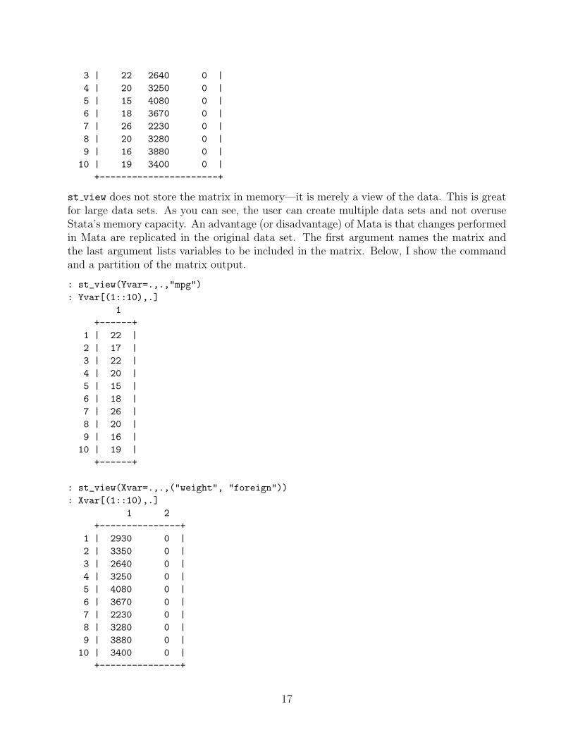
st view does not store the matrix in memory—it is merely a view of the data. This is greatfor large data sets. As you can see, the user can create multiple data sets and not overuseStata’s memory capacity. An advantage (or disadvantage) of Mata is that changes performedin Mata are replicated in the original data set. The first argument names the matrix andthe last argument lists variables to be included in the matrix. Below, I show the commandand a partition of the matrix output.

: st_view(Yvar=.,.,"mpg"): Yvar[(1::10),.]

1+------+

1 | 22 |2 | 17 |3 | 22 |4 | 20 |5 | 15 |6 | 18 |7 | 26 |8 | 20 |9 | 16 |

10 | 19 |+------+

: st_view(Xvar=.,.,("weight", "foreign")): Xvar[(1::10),.]

1 2+---------------+

1 | 2930 0 |2 | 3350 0 |3 | 2640 0 |4 | 3250 0 |5 | 4080 0 |6 | 3670 0 |7 | 2230 0 |8 | 3280 0 |9 | 3880 0 |

10 | 3400 0 |+---------------+

17

: end-----------------------------------------------------------------------------

3 Matrix Algebra in Stata

Above, I showed how to perform matrix algebra in Stata, using the Mata prompt. Below, Ishow how to perform the same exercises while working directly with Stata (note: althoughmatrices below may have the same name as above, they are not necessarily the same). Theuser should pay attention to the additional lines of code required to return a Matrix andthe additional commands required to perform the same exercises. Although this may seeminsignificant for the first-time user, it will become monotonous and unnecessarily repetitiveover time. Notice, above, that I have already ended the Mata session before beginning theexercises using Stata commands. Because I find Mata to be more efficient, I will not spendtoo much text dedicated to explaining matrix manipulations in Stata.

3.1 Creating Matrices

Creating a matrix in Stata is very similar to Mata. The column– and row–join operators arethe same. However, the user must use a command to perform matrix exercises, whereas theuser in Mata can work interactively. As is always the case in Stata, the user can abbreviatecommands. To define a matrix, the user must begin with the matrix command. To list amatrix, the user must use matrix list followed by the name of the matrix defined usingmatrix.

3.1.1 Row Vector

. matrix B = (3,2,6)

. mat list BB[1,3]

c1 c2 c3r1 3 2 6

3.1.2 Column Vector

. matrix A = (2\4\7\3)

. mat list A

A[4,1]c1

18

r1 2r2 4r3 7r4 3

3.1.3 Complex Matrices

Building a more complex matrix in Stata follows the same procedures in Mata, but requiresa command.

. matrix J = 2,3,1,5\54,21,33,29\23,8,99,2\12,45,29,77

. mat list J

J[4,4]c1 c2 c3 c4

r1 2 3 1 5r2 54 21 33 29r3 23 8 99 2r4 12 45 29 77

3.1.4 Combine Matrices

Combining matrices in Stata uses the same notation in Mata; however, the matrix must bedefined using matrix. Here, I create a matrix with row vector B and column vector A.

. matrix G = (B\(23,10,9)\(2,7,92)\(43,89,1)),A

. mat list G

G[4,4]c1 c2 c3 c1

r1 3 2 6 2r2 23 10 9 4r3 2 7 92 7r4 43 89 1 3

3.1.5 matuniform()

matuniform pulls random draws from uniform[0,1] to fill elements in a matrix, just likeuniform in Mata.

. matrix H = matuniform(3,4)

. mat list H

19

H[3,4]c1 c2 c3 c4

r1 .52276946 .21022287 .55345639 .9088587r2 .27698879 .39152514 .03965652 .42354259r3 .6125947 .50159436 .47206923 .81977622

3.1.6 Transposition

Just like Mata, Stata follows writing convention for transposing matrices.

. mat At = A’

. mat list A

A[4,1]c1

r1 2r2 4r3 7r4 3. mat list At

At[1,4]r1 r2 r3 r4

c1 2 4 7 3

. mat Gt = G’

. mat Gtt = G’’

. mat list G

G[4,4]c1 c2 c3 c1

r1 3 2 6 2r2 23 10 9 4r3 2 7 92 7r4 43 89 1 3

. mat list Gt

Gt[4,4]r1 r2 r3 r4

c1 3 23 2 43c2 2 10 7 89c3 6 9 92 1c1 2 4 7 3

20

. mat list Gtt

Gtt[4,4]c1 c2 c3 c1

r1 3 2 6 2r2 23 10 9 4r3 2 7 92 7r4 43 89 1 3

3.1.7 Submatrix

Creating matrix partitions in Stata is more difficult than in Mata. For this reason, I onlyshow one example of calling an element from a matrix.

. mat Gelement = G[3,2]

. mat list Gelement

symmetric Gelement[1,1]c1

r1 7

3.2 Types of Matrices

Stata can develop a variety of different types of matrices, many of which replicate the nomen-clature used in Mata. Although this list is not exhaustive, it provides a sample of what Statacan do in regards to creating different types of matrices.

3.2.1 Matrix of Constants

J() takes three arguments to create a matrix of constants.

. matrix C = J(4,3,5)

. mat list C

C[4,3]c1 c2 c3

r1 5 5 5r2 5 5 5r3 5 5 5r4 5 5 5

21

3.2.2 Null Matrix

Use J() to create a null matrix.

. matrix N = J(4,4,0)

. mat list N

symmetric N[4,4]c1 c2 c3 c4

r1 0r2 0 0r3 0 0 0r4 0 0 0 0

3.2.3 Unit Matrix

Use J() to create a unit matrix.

. matrix U = J(3,2,1)

. mat list U

U[3,2]c1 c2

r1 1 1r2 1 1r3 1 1

3.2.4 Identity Matrix

I() takes one argument that identities the length of the diagonal to create an identitymatrix.

. matrix I = I(4)

. mat list I

symmetric I[4,4]c1 c2 c3 c4

r1 1r2 0 1r3 0 0 1r4 0 0 0 1

22

3.2.5 Scalar Matrix

Multiple the identity matrix by a scalar to create a scalar matrix.

. matrix S = 8*I(4)

. mat list S

symmetric S[4,4]c1 c2 c3 c4

r1 8r2 0 8r3 0 0 8r4 0 0 0 8

3.2.6 Diagonal Matrix

Stata users can easily convert a row or column vector into a diagonal matrix using diag().However, the same cannot be said when converting other matrices into a diagonal ma-trix.

. matrix Ad = diag(A)

. mat list Ad

symmetric Ad[4,4]r1 r2 r3 r4

r1 2r2 0 4r3 0 0 7r4 0 0 0 3

3.2.7 Diagonal Matrix Continued—Extract Diagonal into Row Vector

To convert a square matrix into a diagonal matrix, the user must first extract the diagonalas a row vector—vecdiag(). Next, the user can convert the row vector into a diagonalmatrix—diag().

. matrix Gdrow = vecdiag(G)

. mat list Gdrow

Gdrow[1,4]c1 c2 c3 c1

r1 3 10 92 3

23

. matrix Gdiag = diag(Gdrow)

. mat list Gdiag

symmetric Gdiag[4,4]c1 c2 c3 c1

c1 3c2 0 10c3 0 0 92c1 0 0 0 3

The user can combine commands to make this process faster and more efficient.

. matrix Gnewdiag = diag(vecdiag(G))

. mat list Gnewdiag

symmetric Gnewdiag[4,4]c1 c2 c3 c1

c1 3c2 0 10c3 0 0 92c1 0 0 0 3

3.2.8 Symmetric Matrix

As you can see, constructing a symmetric matrix follows the same steps as any other ma-trix.

. matrix K = (1,3,5\3,7,4\5,4,9)

. mat Kt = K’

. mat list K

symmetric K[3,3]c1 c2 c3

r1 1r2 3 7r3 5 4 9

. mat list Kt

symmetric Kt[3,3]r1 r2 r3

c1 1c2 3 7c3 5 4 9

24

3.3 Matrix Algebra

3.3.1 Addition

. mat addGJ = G+J

. mat list addGJ

addGJ[4,4]c1 c2 c3 c4

r1 5 5 7 7r2 77 31 42 33r3 25 15 191 9r4 55 134 30 80

3.3.2 Subtraction

. mat subGJ = G-J

. mat list subGJ

subGJ[4,4]c1 c2 c3 c4

r1 1 -1 5 -3r2 -31 -11 -24 -25r3 -21 -1 -7 5r4 31 44 -28 -74

3.3.3 Scalar Multiplication

. mat scaleG = 5*G

. mat list scaleG

scaleG[4,4]c1 c2 c3 c1

r1 15 10 30 10r2 115 50 45 20r3 10 35 460 35r4 215 445 5 15

3.3.4 Matrix Multiplication

. mat mulGJ = G*J

25

. mat list mulGJ

mulGJ[4,4]c1 c2 c3 c4

r1 276 189 721 239r2 841 531 1360 731r3 2582 1204 9544 936r4 4951 2141 3166 3029

. mat mulJG = J*G

. mat list mulJG

mulJG[4,4]c1 c2 c3 c1

r1 292 486 136 38r2 1958 3130 3578 510r3 537 997 9320 777r4 4440 7530 3222 638

Multiply elements.

. mat eleHG = H[1,1]*G[1,2]

. mat list eleHG

symmetric eleHG[1,1]c1

r1 1.0455389

3.3.5 Determinant

. mat detG = det(G)

. mat list detG

symmetric detG[1,1]c1

r1 171232

. mat detK = det(K)

. mat list detK

symmetric detK[1,1]c1

26

r1 -89

3.3.6 (Square) Matrix Inversion

. mat invG = inv(G)

. mat list invG

invG[4,4]r1 r2 r3 r4

c1 -.14375818 .07131845 .00245281 -.00497571c2 .04072837 -.0311332 .00023944 .01379999c3 -.06650626 .00853812 .01437815 -.00059568c1 .87442768 -.10145884 -.04705312 -.00454938

. mat invGJ = inv(G*J)

. mat list invGJ

invGJ[4,4]r1 r2 r3 r4

c1 .18066769 -.07533285 -.00469726 .00537649c2 -3.2925828 1.3302289 .08857451 -.08860211c3 .18630565 -.07498131 -.00491512 .00491411c4 1.8372698 -.73874427 -.04979222 .04903271

. mat invGt = inv(G)’

. mat list invGt

invGt[4,4]c1 c2 c3 c1

r1 -.14375818 .04072837 -.06650626 .87442768r2 .07131845 -.0311332 .00853812 -.10145884r3 .00245281 .00023944 .01437815 -.04705312r4 -.00497571 .01379999 -.00059568 -.00454938

AA−1 = A−1A = I

. mat GinvG = G*inv(G)

. mat list GinvG

symmetric GinvG[4,4]

27

r1 r2 r3 r4r1 1r2 0 1r3 -6.661e-16 2.776e-17 1r4 -2.220e-16 -4.163e-16 2.082e-17 1

3.3.7 Rows and Columns

Quickly count the number of rows and columns in an unknown dimensional matrix.

. mat numrow = rowsof(H)

. mat list numrow

symmetric numrow[1,1]c1

r1 3

. mat numcol = colsof(H)

. mat list numcol

symmetric numcol[1,1]c1

r1 4

3.4 Data as Matrices

The user can convert data in Stata’s memory into a matrix and save a matrix as variablesin a data set as columns.

mkmat converts data in memory as a matrix. The user defines the variables of interest, namesthe matrix, and can include an option that removes rows with missing data.

. mkmat mpg weight foreign, matrix(Var) nomissing

svmat saves variables from a matrix as columns in data stored in Stata’s memory. The userdefines the prefix of the variable, which is followed by a number.

. svmat Var, names(Var)

28

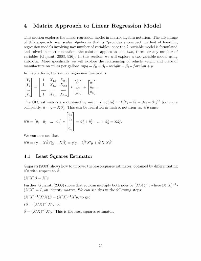
4 Matrix Approach to Linear Regression Model

This section explores the linear regression model in matrix algebra notation. The advantageof this approach over scalar algebra is that is “provides a compact method of handlingregression models involving nay number of variables; once the k–variable model is formulatedand solved in matrix notation, the solution applies to one, two, three, or any number ofvariables (Gujarati 2003, 926). In this section, we will explore a two-variable model usingauto.dta. More specifically we will explore the relationship of vehicle weight and place ofmanufacture on miles per gallon: mpg = β0 + β1 ∗ weight+ β2 ∗ foreign+ µ.

In matrix form, the sample regression function is:Y1

Y2

...Yn

=

1 X1,1 X2,1

1 X1,2 X2,2

..... ..... .....1 X1,n X2,n

∗β1

β2

β3

+

u1

u2

un

.

The OLS estimators are obtained by minimizing Σu2i = Σ(Yi − β1 − β2,i − β3,i)

2 (or, more

compactly, u = y −Xβ). This can be rewritten in matrix notation as: u′u since

u′u =[u1 u2 ... un

]∗

u1

u2

...un

= u21 + u2

2 + ...+ u2n = Σu2

i .

We can now see that

u′u = (y −Xβ)′(y −Xβ) = y′y − 2β′X ′y + β′X ′Xβ

4.1 Least Squares Estimator

Gujarati (2003) shows how to uncover the least-squares estimator, obtained by differentiatingu′u with respect to β:

(X ′X)β = X ′y

Further, Gujarati (2003) shows that you can multiply both sides by (X ′X)−1, where (X ′X)−1∗(X ′X) = I, an identity matrix. We can see this in the following steps:

(X ′X)−1(X ′X)β = (X ′X)−1X ′y, to get

Iβ = (X ′X)−1X ′y, or

β = (X ′X)−1X ′y. This is the least squares estimator.

29

4.2 RSS, TSS, and ESS

We know that the Residual Sum of Squares = Total Sum of Squares - Explained Sumof Squares. The formulas can be derived using this basic two-variable formula: Σu2

i =Σy2

i − β22Σx2

i , which can be extended to the k-variable model: Σu2i = Σy2

i − β2Σyix2,i− . . .−βkΣyixk,i. From here, we can derive the RSS, TSS, and ESS in matrix notation..

TSS = Σy2i = y′y − nY 2

ESS = β2Σyix2,i + . . .+ βkΣyixk,i = β′X ′y − nY 2

RSS = u′u = y′y − β′X ′y

4.3 Variance-Covariance Matrix

Now that we have the formula for RSS. We can derive the variance-covaraiance matrix forβ. Gujarati (2003) shows that var − cov(β) = σ2(X ′X)−1, where σ2 =

Σu2i

n−k. So,

var − cov(β) =Σu2

i

n−k(X ′X)−1, which

= RSSn−k

(X ′X)−1

The user can extract the diagonal and find the the square root to uncover the standard errorof each estimator.

4.4 An Illustration using Auto.dta

As you can see from above, performing matrix calculations in Stata are much more intensivethan in Mata. In response to the efficiency of Mata, I will be evaluating the Matrix LinearRegression Model in Mata. These steps can be adapted for Stata. To start, I clear Stata’smemory and Mata’s memory.

. clear

4.4.1 Prepare the Data

The user must first prepare the data for analysis. This is first accomplished in the Stataprompt, where the user uploads data into Stata’s memory.

. use http://www.stata-press.com/data/r9/auto.dta, clear /* bring in data */(1978 Automobile Data)

Next, the user generates a variable equal to one that will be used in matrix calculations toderive the y-intercept, or β0. Call this variable constant.

. gen constant = 1

30

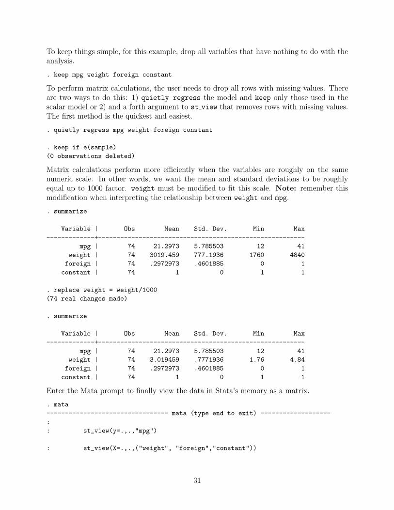
To keep things simple, for this example, drop all variables that have nothing to do with theanalysis.

. keep mpg weight foreign constant

To perform matrix calculations, the user needs to drop all rows with missing values. Thereare two ways to do this: 1) quietly regress the model and keep only those used in thescalar model or 2) and a forth argument to st view that removes rows with missing values.The first method is the quickest and easiest.

. quietly regress mpg weight foreign constant

. keep if e(sample)(0 observations deleted)

Matrix calculations perform more efficiently when the variables are roughly on the samenumeric scale. In other words, we want the mean and standard deviations to be roughlyequal up to 1000 factor. weight must be modified to fit this scale. Note: remember thismodification when interpreting the relationship between weight and mpg.

. summarize

Variable | Obs Mean Std. Dev. Min Max-------------+--------------------------------------------------------

mpg | 74 21.2973 5.785503 12 41weight | 74 3019.459 777.1936 1760 4840foreign | 74 .2972973 .4601885 0 1constant | 74 1 0 1 1

. replace weight = weight/1000(74 real changes made)

. summarize

Variable | Obs Mean Std. Dev. Min Max-------------+--------------------------------------------------------

mpg | 74 21.2973 5.785503 12 41weight | 74 3.019459 .7771936 1.76 4.84foreign | 74 .2972973 .4601885 0 1constant | 74 1 0 1 1

Enter the Mata prompt to finally view the data in Stata’s memory as a matrix.

. mata--------------------------------- mata (type end to exit) -------------------:: st_view(y=.,.,"mpg")

: st_view(X=.,.,("weight", "foreign","constant"))

31

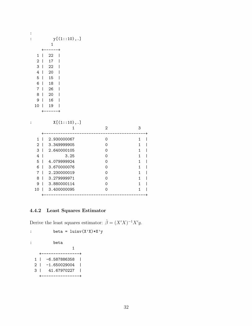
:: y[(1::10),.]

1+------+

1 | 22 |2 | 17 |3 | 22 |4 | 20 |5 | 15 |6 | 18 |7 | 26 |8 | 20 |9 | 16 |

10 | 19 |+------+

: X[(1::10),.]1 2 3

+-------------------------------------------+1 | 2.930000067 0 1 |2 | 3.349999905 0 1 |3 | 2.640000105 0 1 |4 | 3.25 0 1 |5 | 4.079999924 0 1 |6 | 3.670000076 0 1 |7 | 2.230000019 0 1 |8 | 3.279999971 0 1 |9 | 3.880000114 0 1 |

10 | 3.400000095 0 1 |+-------------------------------------------+

4.4.2 Least Squares Estimator

Derive the least squares estimator: β = (X ′X)−1X ′y.

: beta = luinv(X’X)*X’y

: beta1

+----------------+1 | -6.587886358 |2 | -1.650029004 |3 | 41.67970227 |

+----------------+

32

4.4.3 RSS, TSS, and ESS

Derive RSS, TSS, and ESS.

TSS: Σy2i = y′y − nY 2

: tss = y’y-rows(y)*mean(y)^2

: tss2443.459459

ESS: β2Σyix2,i + . . .+ βkΣyixk,i = β′X ′y − nY 2

: ess = beta’X’y-rows(y)*mean(y)^2

: ess1619.287731

RSS: u′u = y′y − β′X ′y

: rss = y’y-beta’X’y

: rss824.1717287

Show that RSS = TSS - ESS

: tss - ess824.1717287

Now that you have ESS and TSS, you can uncover R2.

: r2 = ess/tss

: r2.662702925

4.4.4 Variance-Covariance Matrix

Now that you have RSS, the user can easily derive the variance-covariance matrix of β:= RSS

n−k(X ′X)−1

: varcov = (rss/(rows(y)-cols(X)))*luinv(X’X)

: varcov1 2 3

+----------------------------------------------+1 | .4059128628 .4064025078 -1.346459802 |2 | .4064025078 1.157763273 -1.57131579 |3 | -1.346459802 -1.57131579 4.689594304 |

+----------------------------------------------+

33

The user can extract the diagonal for the variance and derive the square root to uncover thestandard error for each estimator.

: variance = diagonal(diag(varcov))

: variance1

+---------------+1 | .4059128628 |2 | 1.157763273 |3 | 4.689594304 |

+---------------+

: se = sqrt(variance)

: se1

+---------------+1 | .6371129122 |2 | 1.075994086 |3 | 2.165547114 |

+---------------+

4.4.5 Results

Display the final results.

: beta1

+----------------+1 | -6.587886358 |2 | -1.650029004 |3 | 41.67970227 |

+----------------+

: se1

+---------------+1 | .6371129122 |2 | 1.075994086 |3 | 2.165547114 |

+---------------+

: r2.662702925

34

4.4.6 Compare to Stata Output using regress

Compare the results using the Matrix Linear Regression Model in Mata to the results usingthe Scalar Linear Regression Model in Stata. the user can see that the estimators, standarderrors, t-ratios, and p-values are all the same.

: (beta, se, beta:/se, 2*ttail(rows(y)-cols(X), abs(beta:/se)))1 2 3 4

+-------------------------------------------------------------+1 | -6.587886358 .6371129122 -10.34021793 8.28286e-16 |2 | -1.650029004 1.075994086 -1.533492633 .1295987129 |3 | 41.67970227 2.165547114 19.24673077 6.89556e-30 |

+-------------------------------------------------------------+

:: end-----------------------------------------------------------------------------

.

. regress mpg weight foreign

Source | SS df MS Number of obs = 74-------------+------------------------------ F( 2, 71) = 69.75

Model | 1619.28773 2 809.643865 Prob > F = 0.0000Residual | 824.171729 71 11.6080525 R-squared = 0.6627

-------------+------------------------------ Adj R-squared = 0.6532Total | 2443.45946 73 33.4720474 Root MSE = 3.4071

------------------------------------------------------------------------------mpg | Coef. Std. Err. t P>|t| [95% Conf. Interval]

-------------+----------------------------------------------------------------weight | -6.587886 .6371129 -10.34 0.000 -7.858253 -5.317519foreign | -1.650029 1.075994 -1.53 0.130 -3.7955 .4954423_cons | 41.6797 2.165547 19.25 0.000 37.36172 45.99768

------------------------------------------------------------------------------

References

Gujarati, D.N. 2003. Basic Econometrics. McGraw Hill, New York.

35