a bayesian analysis of the 69 highest energy cosmic … · a bayesian analysis of the 69 highest...

Mon. Not. R. Astron. Soc. 000, 1–14 (2016) Printed 2nd May 2018 (MN LATEX style file v2.2)

A Bayesian analysis of the 69 highest energy cosmic raysdetected by the Pierre Auger Observatory

Alexander Khanin1? and Daniel J. Mortlock1,2

1Astrophysics Group, Imperial College London, Blackett Laboratory, Prince Consort Road, London SW7 2AZ, U.K.2Department of Mathematics, Imperial College London, London SW7 2AZ, U.K.

Accepted 2016 ?????? ??. Received 2016 ?????? ??; in original form 2016 ???????? ??

ABSTRACTThe origins of ultra-high energy cosmic rays (UHECRs) remain an open question. Sev-eral attempts have been made to cross-correlate the arrival directions of the UHECRswith catalogs of potential sources, but no definite conclusion has been reached. Wereport a Bayesian analysis of the 69 events from the Pierre Auger Observatory (PAO),that aims to determine the fraction of the UHECRs that originate from known AGNs inthe Veron-Cety & Veron (VCV) catalog, as well as AGNs detected with the Swift BurstAlert Telescope (Swift-BAT), galaxies from the 2MASS Redshift Survey (2MRS), andan additional volume-limited sample of 17 nearby AGNs. The study makes use of amulti-level Bayesian model of UHECR injection, propagation and detection. We findthat for reasonable ranges of prior parameters, the Bayes factors disfavour a purelyisotropic model. For fiducial values of the model parameters, we report 68% cred-ible intervals for the fraction of source originating UHECRs of 0.09+0.05

−0.04, 0.25+0.09−0.08,

0.24+0.12−0.10, and 0.08+0.04

−0.03 for the VCV, Swift-BAT and 2MRS catalogs, and the sampleof 17 AGNs, respectively.

Key words: cosmic rays – methods: statistical

1 INTRODUCTION

Cosmic rays (CRs) are highly accelerated protons andatomic nuclei, some of which enter the Solar system andreach the Earth. They are the most energetic particles ob-served in nature, with energies in the range 109 eV to 1021 eV(see e.g. Kotera & Olinto 2011, Letessier-Selvon & Stanev2011 for reviews).

A number of open scientific issues remain with re-spect to CRs, in particular ultra-high energy cosmic rays(UHECRs) with arrival energies Earr & 1019 eV. The studyof UHECRs is complicated by the fact that they experiencean abrupt cutoff in their energy spectrum at∼ 4×1019 eV, sothat only small samples are available. The largest currentlyavailable sample is the 69 events with Earr > 5.5 × 1019 eVrecorded by the Pierre Auger Observatory (PAO) between2004 January 1 and 2009 December 31 (Abreu et al. 2010).

One open issue in the study of UHECRs is the ques-tion of their sources. A number of candidates, such as activegalactic nuclei (AGNs) and pulsars have been proposed, butstudies have not been conclusive (see e.g. Kalmykov et al.2013 for a review). The question of UHECR origins canbe studied by attempting to associate the arrival directions

? E-mail: [email protected]

with their sources. While UHECRs are charged particles andtherefore experience magnetic deflection as they propagate,they are sufficiently energetic that the total deflection is ex-pected to be ∼ 2 to ∼ 10 deg (e.g. Medina Tanco et al. 1998;Sigl et al. 2004; Dolag et al. 2005), so that some informationabout their points of origin should be retained.

Association of UHECRs with catalogs of potentialsources is made possible by the fact that UHECRs with en-ergies of E & 5× 1019 eV are expected to have come from alimited radius of ∼ 100 Mpc. This radius is sometimes calledthe Greisen-Zatsepin-Kuzmin (GZK) horizon, and arises dueto the fact that UHECRs at those energies scatter off thecosmic microwave background (CMB) radiation in a processknown as the GZK effect (Greisen 1966, Zatsepin & Kuzmin1966). The mean free path of the GZK effect at high energiesis a few Mpc and the energy loss in each collision is 20-50%.The resultant attenuation is very rapid, and is the cause ofthe cutoff in the UHECR energy spectrum observed by bothHiRes (Abbasi et al. 2008) and PAO (Abraham et al. 2008).

A number of attempts have been made to find correl-ations between UHECR arrival directions and catalogs ofpossible sources. Cross-correlation studies have been con-ducted with galaxy catalogs, such as the Two Micron All-Sky Survey (2MASS) Redshift Survey (2MRS) (Abrahamet al. 2009; Abbasi et al. 2010), as well as specific types

c© 2016 RAS

arX

iv:1

601.

0230

5v1

[as

tro-

ph.H

E]

11

Jan

2016

2 A. Khanin & D. J. Mortlock

of objects such as active galactic nuclei (AGNs) (Abrahamet al. 2007; Abraham et al. 2008; George et al. 2008; Pe’Eret al. 2009; Watson et al. 2011) and BL Lacertae objects(BL LAcs) (Tinyakov & Tkachev 2001). Overall, no clearconsensus has been reached. Different studies have reporteddifferent degrees of correlation, depending on the statisticalapproach, the UHECR sample, and the population of sourcecandidates that was used. The most significant correlationwas reported by the Pierre Auger Collaboration, between ar-rival directions of UHECRs with energies E > 5.7× 1019 eVand the positions of nearby AGNs (Abraham et al. 2007).The result was supported by Yakutsk data (Ivanov 2009),but not by HiRes (Abbasi et al. 2008) or the Telescope Array(Abu-Zayyad et al. 2012). A more recent analysis of a lar-ger PAO sample has shown a weaker correlation than before(Abreu et al. 2010).

The lack of consensus on these issues is partly due tothe difficulty of analyzing such small sample sizes. Given thesmall size of the UHECR data sets, it is important to utilizeas much of the available information as possible. This can beachieved by adopting a Bayesian methodology, that involvesmodels of the relevant physical processes. The first stepsto such a comprehensive Bayesian work have been made inthe recent work of Watson et al. (2011) and Soiaporn et al.(2013).

Watson et al. (2011) analysed the 27 events that wereanalysed in Abraham et al. (2007), and derived a posteriorfor the fraction that originated from AGNs in the Veron-Cetty & Veron (VCV) catalog (Veron-Cetty & Veron 2006).To do so, they used a two-component parametric modelcharacterized by a source rate Γ and a background UHECRrate R. The model assumed that the UHECR arrival direc-tions are points drawn from a Poisson intensity distributionon the celestial sphere. The intensity distribution was ob-tained with a computational UHECR model. Watson et al.(2011) report strong evidence of a UHECR signal from theVCV AGNs. They find a low AGN fraction that is consist-ent with Abreu et al. (2010). For fiducial values of the modelparameters, they report a 68% credible interval for the AGNfraction of FAGN = 0.15+0.10

−0.07.

Soiaporn et al. (2013) developed a multi-level Bayesianframework to attempt to associate the 69 UHECRs thatwere recorded at the PAO in the period 2004-2009 with 17nearby AGNs catalogued by Goulding et al. (2010) (here-after G10). They report evidence for a small but nonzerofraction of the UHECRs to have originated at the AGNsfrom G10, of the order of a few percent to 20%.

We extend the formalism of Watson et al. (2011) withboth a greater data set and a refined UHECR model. Follow-ing Abreu et al. (2010), we extend the analysis to two furthersource catalogs: AGNs from the Swift Burst Alert Telescope(Swift-BAT) (Baumgartner et al. 2010) and galaxies from2MRS (Huchra et al. 2012). We also extend the analysis tothe 17 AGNs from the G10 catalog.

After discussing the UHECR and source data sets inSection 2, we explain our UHECR model in Section 3, dis-cuss the statistical formalism of our Bayesian model com-parison in Section 4, and the application of the formalismto mock data sets in Section 5. The results of applyingthe formalism to the PAO data are discussed in Section 6.Some aspects of our computational approach are describedin Appendix A, and some subtleties of our model compar-

ison are explored in Appendix B. We use a Hubble constantof H0 = 70 km/s/Mpc where required to convert betweenredshifts and distances.

2 DATA

2.1 UHECR sample

The sample of UHECR events that was used in this ana-lysis were the 69 highest energy events recorded at thePAO between January 2004 and November 2009, as doc-umented in Abreu et al. (2010). These are the events withobserved energies Eobs above the threshold Eobs > Ethres =5.7× 1019 eV.

The PAO is a CR observatory located in Argentina, ata longitude of 69.5 W and a latitude 35.2 S. PAO is ahybrid observatory, which means that it uses both surfacedetection (SD) and fluorescent telescope detection (FD) ofUHECRs. The observatory has SD plastic scintillators of atotal area of 3000 km2 and 4 FD telescopes.

The PAO’s total exposure of this data-set is εtot =20, 370 km2 sr yr and its relative exposure per unit solidangle, dε/dΩ, is illustrated in Figure 1. The relative expos-ure is directly proportional to Pr(det|r), the probability thata UHECR will be detected if it arrives from direction r, butis normalized so that

∫(dε/dΩ) dΩ = εtot.

PAO measures UHECR arrival directions with an un-certainty of ∼ 1 deg and arrival energies with a relative un-certainty of ∼ 12% (Letessier-Selvon et al. 2014).

2.2 Source catalogs

As potential source catalogs, we consider AGNs from theVCV, Swift-BAT and G10 catalogs, and galaxies from the2MRS catalog. This allows us to compare our analysis forthe Swift-BAT and 2MRS sources with the analysis fromAbreu et al. (2010), our analysis for the VCV sources withthe analyses from both Abreu et al. (2010) and Watson et al.(2011), and our analysis of the G10 sources with Soiapornet al. (2013).

We use the 12th edition of the VCV catalog, selectingsources with zobs 6 0.03, as AGNs with higher redshift aretoo far away to be plausible UHECR sources, and can beshown to have a negligible effect on the results. We omitsources for which absolute magnitudes are not stated. Thetotal number of VCV AGNs that meet those requirementsis NVCV = 921. This is the same sample of sources thatwas used in Abraham et al. (2007), Abreu et al. (2010) andWatson et al. (2011), and in PAO’s more recent analysis Aabet al. (2015). While the VCV catalog is heterogenous andthus not ideal for statistical studies, it is close to completefor the low-redshift AGNs that are of relevance here.

For the Swift-BAT catalog, we use the 58 month ver-sion, that includes a total of NBAT = 1092 sources. In thecase of the 2MRS catalog, we used the catalog version 2.4,2011 Dec 16. We exclude events that are within 10 of theGalactic plane, to avoid biases due to the incompleteness ofthe catalog in the region of the Galactic plane. This leavesa total of N2MRS = 20, 702 galaxies. These samples of Swift-BAT and 2MRS sources are the same as those used by Abreuet al. (2010).

c© 2016 RAS, MNRAS 000, 1–14

Bayesian analysis of cosmic rays 3

0.05 0.1 0.2 0.5

Figure 1. Relative PAO exposure in Galactic coordinates. The arrival directions of the 69 UHECRs are shown as black points. TheGalactic centre (GC) and south celestial pole (SCP) are indicated.

(A) VCV (B) Swift-BAT

(C) 2MRS (D) G10

0.05 0.1 0.2 0.5

Figure 2. Positional dependence of the expected number of source originating events, for the VCV, Swift-BAT, 2MRS, and G10 catalogs.

A fiducial value of the smearing parameter σ = 3 deg is assumed. The arrival directions of the 69 UHECRs are shown as black points.

Galactic coordinates are used, and the Galactic centre (GC) and south celestial pole (SCP) are indicated.

The G10 catalog is a well-characterized volume-limitedsample of AGNs. The 17 AGNs contained in it constituteall infrared-bright AGNs within 15 Mpc. This is the samesample that was used by Soiaporn et al. (2013).

3 UHECR MODEL

A Bayesian UHECR analysis requires a realistic model ofUHECR injection, propagation, and detection. This modelwas used both to compute the likelihoods in our statistical

formalism (Section 4), and to create simulated mock catalogsof UHECRs to test our methods (Section 5).

3.1 Injection

We adopt a model in which any given UHECR source emitsUHECRs with an emission spectrum given by

dNemit/dEemit ∝ E−γ−1emit , (1)

where the logarithmic slope γ is taken to be 3.6 (Abrahamet al. 2010). The spectrum is normalized in such a way that

c© 2016 RAS, MNRAS 000, 1–14


the total emission rate of UHECRs with energy greater thanEemit is given by

dNemit(> Eemit)

dt= Γs

(Eemit

Emin

)−γ, (2)

where Emin = 5.7× 1019 eV is the minimum UHECR emis-sion energy and Γs is the rate at which source s emitsUHECRs with Eemit > Emin.

3.2 Energy loss during propagation

The energy loss processes experienced by UHECRs canbe characterized in terms of the loss length Lloss =−E(dE/dr)−1. Given the loss length as a function of en-ergy, it is possible to calculate the total amount of energythat a UHECR loses as it travels to the Earth from a givendistance by solving the differential equation

dE

dr= − E

Lloss(E). (3)

For pure proton composition, Lloss obeys the expression

L−1loss =

1

c[βadi(E, z) + βGZK(E, z) + βBH(E, z)], (4)

where c is the speed of light and βGZK(E, z), βBH(E, z) andβadi(E, z) are terms corresponding to the three main energyloss processes experienced by UHECRs of pure proton com-position (e.g. Stanev 2009):

(i) the GZK scattering off the CMB photons at energiesabove E & 5× 1019 eV;

(ii) Bethe-Heitler (BH) e+e− pair production (also a scat-tering process off the CMB radiation), which dominates atlower energies (Hillas 1968);

(iii) the adiabatic energy loss due to the expansion of theUniverse.

A detailed discussion of these terms, including expressionsand parametrizations, can be found in De Domenico & Inso-lia (2013). For the energies that are relevant in this investig-ation, the dominant term is βGZK(E, z). The Bethe-Heitlerand adiabatic processes dominate the energy loss at lowerenergies, but play only a minor role at the higher energiesin question.

The loss lengths are shown as a function of energy inFigure 3. The contributions to the loss length from the BHand adiabatic losses are combined into a single functionLadi,BH that is contrasted with the loss length due to theGZK effect, LGZK. The two are combined into the total losslength Ltot. The figure shows Ltot plots for z values of 0.0and 0.1, which correspond to distances of 0 and ∼ 400 Mpc,thus covering the GZK horizon. LGZK appears very rapidlyafter an energy of ∼ 4 × 1019 eV and begins to dominatethe energy loss. As we are interested only in UHECRs withenergies Eobs > Ethres = 5.7× 1019 eV, the GZK scatteringis the most relevant loss process in this investigation.

The energy dependence of Lloss(E) is one of the mainimprovements of this propagation model over the model usedin Watson et al. (2011), where Lloss was taken to be a con-stant. The constant value of Lloss used by Watson et al.(2011) is also displayed in Figure 3 for comparison.

1019 1020 1021 1022

E / eV

100

101

102

103

104

L/

Mpc

Ethres

Ltot

Ltot, Watson et al.

Ltot for z=0.1

LGZK

Ladi,BH

Figure 3. Loss lengths from the three energy loss processes, com-

pared to the constant constant loss length used by Watson et al.(2011), as described in Section 3.2.

3.3 Effective smearing

We combined the magnetic deflection that a UHECR experi-ences during propagation and the uncertainty in its detectedarrival direction into a single kernel, which was chosen to bea von Mises-Fisher (vMF) distribution, defined as

Pr(r|rsrc, κ) =κ

4π sinh(κ)exp(κr · rsrc), (5)

where r is the measured arrival direction of the ray, rsrc isthe source direction and κ is the concentration parameter.The vMF distribution resembles a Gaussian on the sphere,with κ being inversely related to the width of the Gaussian:for large values of κ the distribution is peaked over an angu-lar scale of ∼ 1/

√κ ; if κ tends to 0 the distribution becomes

uniform on the sphere.The magnitude of the deflection that the highest en-

ergy UHECRs experience is uncertain, with the estimates oftypical deflection angles ranging from ∼ 2 to ∼ 10 deg (e.g.Medina Tanco et al. 1998; Sigl et al. 2004; Dolag et al. 2005).We assume a fiducial smearing angle of σ ' 3 deg (κ = 360),but also conduct investigations for smearing angles of σ '6 and 10 deg (κ = 90 and 30).

3.4 Observed UHECR flux

The number of UHECRs from source s above a thresholdenergy Ethres observed on Earth per unit area per unit time,dNs(Eobs > Ethres)/dtdA, is a quantity that is important inour statistical analysis. This rate is proportional to the rateof UHECRs emitted by the source, Γs, but it also dependson the distance-dependence of the UHECR energy loss, andon the UHECR injection spectrum. We use the UHECRpropagation model described in Section 3.2 to determinethe injection energy corresponding to the threshold energyEthres and to the source distance Ds. Combining this valuewith Equation 2 and with the source distance Ds, we obtain

dNs(Eobs > Ethres)

dtdA=

Γs4πD2

s

[Eemit(Ethres)

Emin

]−γ. (6)

c© 2016 RAS, MNRAS 000, 1–14


This expression assumes that the observed energy Eobs isequivalent to the arrival energy of the UHECR, Earr. Thus,for the purposes of the calculation, the 12% energy uncer-tainty of the PAO measurements is neglected. The variationin source rates Γs among the sources that we are consider-ing is not negligible. We use the source rate of CentaurusA as the reference value Γ. The source rate of a source s isobtained by weighing the flux Fs of that source in a par-ticular band against the flux FCen of Centaurus A in thatsame band. The wave band of the flux thereby is differentdepending on the source catalog. For VCV, the flux of thesource in the V -band is used, for Swift-BAT the X-ray flux,for 2MRS the IR flux, for G10 the K-band flux. The fluxesare thus used as weights, so that sources with higher fluxcontribute more UHECRs. This approach is very similar tothe approach used in Abreu et al. (2010), where fluxes wereused to weigh the sources from the Swift-BAT and 2MRScatalogs in the same way. Incorporating the fluxes into theformalism, we obtain the expression

dNs(Eobs > Ethres)

dtdA=

Γ

4πD2Cen

FsFCen

[Eemit(Ethres)

Emin

],−γ

(7)

where DCen is the distance to Centaurus A.

4 STATISTICAL FORMALISM

Given a sample of UHECRs arrival directions, we wouldlike to determine the fraction of these rays that have comefrom a set of sources under consideration. To do so, we usea two-component parametric model characterized by tworates: The source rate Γ and the isotropic background rateR. As elaborated in Section 3.4, we use the source rate ofCentaurus A as the reference value of Γ. We obtain a jointposterior distribution for the two rates:

Pr(Γ,R|d) =Pr(Γ,R) Pr(d |Γ,R)∫∞

0

∫∞0

Pr(Γ,R) Pr(d |Γ,R) dΓ dR, (8)

where Pr(Γ,R) is the prior distribution for Γ and R, andPr(d |Γ,R) is the likelihood (i.e. the probability of obtainingthe data set d given values of Γ and R).

4.1 Prior

We adopt a uniform prior over Γ and R, with Γ> 0, R> 0.This plausibly encodes our ignorance of the two paramet-ers, and, unlike maximum entropy priors, includes a possiblevalue of 0 for both parameters. The maximum values of Γand R are denoted as Γmax and Rmax. We have conductedour analysis for flat priors of varying width, using a vari-able width parameter s. The expression for the prior can bewritten as

Pr(Γ, R|d ,M2) =1

s2ΓmaxRmax. (9)

Γmax and Rmax have been chosen in such a way that whens = 1, the prior covers the 99.7% credible region implied bythe likelihood and an infinitely broad uniform prior. Thisgives a data driven scaling for the rates. The priors andtheir dependence on s are illustrated in Appendix B.

4.2 The likelihood

To compute the likelihood, we use a ‘counts in cells’ ap-proach, in which the sky is divided into 1800 × 3600 =6,480,000 pixels, that are distributed uniformly in right as-cension and declination. Thus, the data set d can be rewrit-ten as a set of counts in each pixel Nc,p.

The likelihood Pr(d |Γ,R) is then given by a product ofthe individual Poisson likelihoods in each pixel, and can bewritten as

Pr(d |Γ,R)

=

Np∏p=1

(Nsrc,p + Nbkg,p)Nc,p exp[−(Nsrc,p + Nbkg,p)]

Nc,p!, (10)

where Nsrc,p and Nbkg,p are the expected counts in pixel pdue to sources and background, respectively. The expectednumber of counts in pixel p that are contributed by thebackground is

Nbkg,p = R

∫p

dε

dΩdΩobs, (11)

where the integral is over the pixel p, and dε/dΩ is the relat-ive exposure (Section 2.1). The expected number of sourceoriginating events in pixel p is

Nsrc,p =

Ns∑s=1

dNs(Eobs > Ethres)

dtdA

∫p

dε

dΩPr(robs |rs) dΩobs, (12)

where the sum is over the sources, Pr(robs |rs) is the vMFdistribution (Equation 5), and dNs(Eobs > Ethres)/dtdA isthe observed UHECR flux discussed in Section 3.4. InsertingEquations 11 and 12 into Equation 10, we arrive at the fulllikelihood.

The positional dependence of Nbkg,p follows the relativeexposure of PAO, as shown in Figure 1. The positional de-pendence of Nsrc,p depends both on the PAO exposure andon the distribution of sources in the given catalog. Figure 2shows the dependence for the four catalogs that are used inthis study. The dependence is dominated by the distributionof local AGNs, by far the strongest source being CentaurusA (l = 309.5, b = 19.4), which previously studies (e.g. Ab-raham et al. 2007) have suggested as the dominant UHECRsource.

The expression for the likelihood can be rearranged toreduce the total number of computations, as described inAppendix A.

4.3 The source fraction

The source fraction1 is defined as the fraction of theUHECRs that are expected to have originated at the sourcesin whichever catalog is under consideration and is given by

Fsrc(Γ, R) =

∑Np

p=1 Nsrc,p∑Np

p=1 Nsrc,p + Nbkg.p

. (13)

1 The source fraction Fsrc is equivalent to the AGN fraction

FAGN used in Watson et al. (2011) but now generalized to al-low for non-AGN progenitors.

c© 2016 RAS, MNRAS 000, 1–14


The posterior for Fsrc can be calculated from the posteriorover the rates as

Pr(Fsrc|d)

=

Γmax∫0

Rmax∫0

Pr(Γ,R|d) δD[Fsrc − Fsrc(Γ,R)] dΓ dR. (14)

Pr(Fsrc|d) is insensitive to Rmax and Γmax provided they aresufficiently large.

4.4 Model comparison

We would like to compare model M1 where all the UHECRsare drawn from a uniform distribution with model M2 wherethe UHECRs are derived from a combination of a back-ground and a source originating component. To do this, weconduct a Bayesian model comparison. For a data set d , andtwo models M1 and M2, the ratio of the marginal likelihoodsfor the two models, termed the Bayes factor, is

B12 =Pr(d |M1)

Pr(d |M2). (15)

In the specific case that is considered here, the modelsare nested: When Γ = 0, model M2 reduces to model M1. Ageneral expression of the Bayes factor in this situation is

B12 =

∫Pr(R|M1) Pr(d |R,M1) dR∫

Pr(Γ, R|M2) Pr(d |Γ, R,M2) dΓ dR. (16)

It can be shown (Dickey 1971) that in the case of such nestedmodels, the expression reduces to

B12 =Pr(Γ = 0|d ,M2)

Pr(Γ = 0|M2). (17)

This expression is known as the Savage-Dickey Density Ra-tio, or SDDR. Qualitatively, this expression means that thenested uniform model is preferred if, within the context ofthe more complicated model, the data result in an increasedprobability that Γ = 0.

5 SIMULATIONS

In order to investigate the constraining power of a data setof 69 events, we apply the method to simulated data sets.We use two extreme cases:

(i) Uniform arrival directions. These rays were drawnfrom a probability distribution that followed the PAO ex-posure.

(ii) UHECRs originating at sources from a catalog. Weconducted simulations for all four of the catalogs. In eachcatalog, the sources were weighted by their fluxes and thePAO exposure. Random sources were then selected, and thepropagation model of Section 3 was used to propagate raysfrom the sources to the Earth.

The posteriors for the source and background rates, aswell as the posteriors for the source fraction, are summar-ized in Figure 4. The posteriors for the uniform and sourcecentred cases are completely disjoint, which demonstratesthat in extreme senarios where all UHECRs originate eitherfrom a uniform background or from a source catalog, a data

set of 69 events should be sufficient to distinguish betweenthe two models. Figure 4 also shows the Bayes factors asfunctions of s for the two cases. The Bayes factors B21

that are displayed are the inverses of the SDDR given inEquation 17, and favour the more complex model for Bayesfactors > 1.

To assess the results of the Bayes factor simulations,we can derive a rough range of plausible values of s fromphysical models, and then look at the behaviour of theBayes factors at those physically plausible values. Plaus-ible models of UHECR injection predict that the UHECRluminosity of a source like Centaurus A is of the order of2.9×1039 erg s−1 ' 1.81×1051 eV (Fraija et al. 2012). If thisis taken as the typical UHECR luminosity of a source, thenfor a UHECR energy range of (5.7−100)×1019 eV, the rangeof source rates can be calculated by dividing the UHECRluminosity by the limiting values of this range. The resultof this calculation is a range of source rates Γ of roughly(2 − 33) × 1030 s−1. The values of s corresponding to thisrange have been marked on Figure 4. (The values are slightlydifferent for each of the simulations. For the sake of clarity,only the values for the uniform simulation are displayed, theothers being broadly similar.) For the sourced case, modelM2 is strongly favoured for all physically plausible values ofs, while for the uniform case, the simple uniform model M1

is favoured for the physically plausible values.

6 RESULTS

The results of the application of the statistical methods de-scribed in Section 4 to the data described in Section 2 areshown in Figures 5 and 6. Figure 5 contrasts the results fromour analysis with the equivalent results from Watson et al.(2011), and with the results for an intermediate case. Theuse of a more refined propagation model leads to a higherposterior probability for lower source rates. The reason forthat is that in Watson’s propagation model, the energy losslength is constant and very small (Figure 3). UHECRs ex-perience more drastic energy loss than in the more realisticmodel, which leads to more distant AGNs being excluded asplausible source candidates. As fewer sources are included,a higher source rate is required to generate the same sampleof UHECRs.

The inclusion of 69 events reduces the extent to whichthe non-uniform model is favoured. This is evident from theposterior of the source fraction, and also from the behava-viour of B21. This result agrees with the results of Abreuet al. (2010), which reported that the full 69 events yieldlower evidence of anisotropy than the earlier study Abra-ham et al. (2007), which analysed 27 events.

Figures 6 shows results for all four of the source cata-logs, and for all values of the smearing parameter. Displayedare the posteriors for the source fraction, as well as plots ofB21 against s. The constraints on the source fraction for allcases are shown in Table 1. The figures and table show thatfor greater smearing, the range of plausible values of Fsrc isincreased, and the most probable value of the source fractionis higher than for the fiducial model of σ = 3 deg. The reasonis that for greater magnetic deflection, the UHECR intens-ity distribution becomes more uniform, so that the uniform

c© 2016 RAS, MNRAS 000, 1–14


0 10 20 30 40

background rate R (sr−1 m−2 s−1 ×10−17 )

0

20

40

60

sourc

e r

ate

Γ(s

rc−

1s−

1×1

030)

(A)

Uniform simulation

VCV simulation

Swift-BAT simulation

2MRS simulation

G10 simulation

0.0 0.2 0.4 0.6 0.8 1.0Fsrc

0

5

10

15

20

Pr(F

src|d

)

(B)

Uniform simulation

VCV simulation


2MRS simulation

G10 simulation

10-4 10-3 10-2 10-1 100 101 102 103 104 105 106

s

10-7

10-3

101

105

109

1013

1017

1021

1025

1029

1033

1037

1041

1045

B21

M2 favouredM1 favoured

(C)

Uniform simulation

VCV simulation


2MRS simulation

G10 simulation

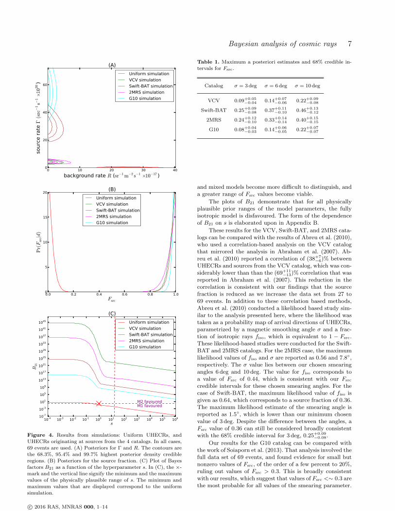
Figure 4. Results from simulations: Uniform UHECRs, andUHECRs originating at sources from the 4 catalogs. In all cases,

69 events are used. (A) Posteriors for Γ and R. The contours arethe 68.3%, 95.4% and 99.7% highest posterior density credibleregions. (B) Posteriors for the source fraction. (C) Plot of Bayesfactors B21 as a function of the hyperparameter s. In (C), the ×-

mark and the vertical line signify the minimum and the maximumvalues of the physically plausible range of s. The minimum and

maximum values that are displayed correspond to the uniformsimulation.

Table 1. Maximum a posteriori estimates and 68% credible in-tervals for Fsrc.

Catalog σ = 3 deg σ = 6 deg σ = 10 deg

VCV 0.09+0.05−0.04 0.14+0.07

−0.06 0.22+0.09−0.08

Swift-BAT 0.25+0.09−0.08 0.37+0.11

−0.10 0.46+0.13−0.12

2MRS 0.24+0.12−0.10 0.33+0.14

−0.14 0.40+0.15−0.15

G10 0.08+0.04−0.03 0.14+0.06

−0.05 0.22+0.07−0.07

and mixed models become more difficult to distinguish, anda greater range of Fsrc values become viable.

The plots of B21 demonstrate that for all physicallyplausible prior ranges of the model parameters, the fullyisotropic model is disfavoured. The form of the dependenceof B21 on s is elaborated upon in Appendix B.

These results for the VCV, Swift-BAT, and 2MRS cata-logs can be compared with the results of Abreu et al. (2010),who used a correlation-based analysis on the VCV catalogthat mirrored the analysis in Abraham et al. (2007). Ab-reu et al. (2010) reported a correlation of (38+7

−6)% betweenUHECRs and sources from the VCV catalog, which was con-siderably lower than than the (69+11

−13)% correlation that wasreported in Abraham et al. (2007). This reduction in thecorrelation is consistent with our findings that the sourcefraction is reduced as we increase the data set from 27 to69 events. In addition to these correlation based methods,Abreu et al. (2010) conducted a likelihood based study sim-ilar to the analysis presented here, where the likelihood wastaken as a probability map of arrival directions of UHECRs,parametrized by a magnetic smoothing angle σ and a frac-tion of isotropic rays fiso, which is equivalent to 1 − Fsrc.These likelihood-based studies were conducted for the Swift-BAT and 2MRS catalogs. For the 2MRS case, the maximumlikelihood values of fiso and σ are reported as 0.56 and 7.8,respectively. The σ value lies between our chosen smearingangles 6 deg and 10 deg. The value for fiso corresponds toa value of Fsrc of 0.44, which is consistent with our Fsrc

credible intervals for these chosen smearing angles. For thecase of Swift-BAT, the maximum likelihood value of fiso isgiven as 0.64, which corresponds to a source fraction of 0.36.The maximum likelihood estimate of the smearing angle isreported as 1.5, which is lower than our minimum chosenvalue of 3 deg. Despite the difference between the angles, aFsrc value of 0.36 can still be considered broadly consistentwith the 68% credible interval for 3 deg, 0.25+0.09

−0.08.

Our results for the G10 catalog can be compared withthe work of Soiaporn et al. (2013). That analysis involved thefull data set of 69 events, and found evidence for small butnonzero values of Fsrc, of the order of a few percent to 20%,ruling out values of Fsrc > 0.3. This is broadly consistentwith our results, which suggest that values of Fsrc <∼ 0.3 arethe most probable for all values of the smearing parameter.

c© 2016 RAS, MNRAS 000, 1–14


0 10 20

background rate R (sr−1 m−2 s−1 ×10−17 )

0

20

sourc

e r

ate

Γ(s

rc−

1s−

1×1

030)

(A)

69 events, variable Lloss


27 events, constant Lloss

0.1 0.2 0.3 0.4 0.5 0.6 0.7 0.8 0.9 1.0Fsrc

0

1

2

3

4

5

6

7

8

Pr(F

src|d

) Fsrc =0.15+0.10−0.07

Fsrc =0.09+0.05−0.04

(B)




10-4 10-3 10-2 10-1 100 101 102 103 104

s

10-5

10-4

10-3

10-2

10-1

100

101

102

103

104

105

106

107

108

109

B21


(C)




Figure 5. Results for σ = 3 deg, and the sources from the VCVcatalog. Results for 27 and 69 events, and for constant and vari-

able loss lengths are displayed. (A) Posteriors for the source andbackground rates. The contours are the 68.3%, 95.4% and 99.7%highest posterior density credible regions. (B) Posterior for thesource fraction. (C) Plot of Bayes factors B21 as a function ofthe hyperparameter s. In (C), physically plausible ranges of s are

shown for the cases of 27 events (blue) and 69 events (black),with a variable loss length. The ×-marks and the vertical linessignify the minimum and the maximum values of the physically

plausible ranges of s.

7 CONCLUSIONS

We have performed a Bayesian analysis of the 69 UHECRsdetected by the PAO with energies Eobs > 5.7 × 1019 eVto determine the fraction of these UHECRs that originatedfrom catalogs of plausible UHECR sources. The sources con-sidered were AGNs from the VCV, Swift-BAT, and G10catalogs, and galaxies from the 2MRS catalog.

For the fiducial magnetic smearing parameter of σ = 3deg, we report 68% credible intervals for the source fractionof 0.09+0.05

−0.04, 0.25+0.09−0.08, 0.08+0.04

−0.03 and 0.24+0.12−0.10 for the VCV,

Swift-BAT, G10 and 2MRS catalogs, respectively. For allphysically plausible values of the model parameters, the fullyuniform model is disfavoured. The results of our study arein broad agreement with previous work on this subject, suchas Watson et al. (2011), Abreu et al. (2010) and Soiapornet al. (2013). The credible intervals for the VCV catalogare lower than the analogous credible intervals from Watsonet al. (2011), which used a similar method to analyse 27 PAOevents. This is consistent with earlier studies: Abreu et al.(2010), which analysed 69 events, reported a lower signalof anisotropy than the earlier study Abraham et al. (2007),which used 27 events.

We will extend this Bayesian framework to include thearrival energies of the UHECRs as well as the arrival direc-tions.

It is expected that future experiments will produce datasets that will be sufficiently large for our Bayesian method(and other statistical approaches; see e.g. Rouille d’Orfeuilet al. 2014) to detect even the weak clustering expected if theUHECRS have come from nearby sources. PAO is continuingto take data and is expected to produce a sample of ∼ 250UHECRs over its first decade of operations. Looking furtherahead, the planned Japanese Experiment Module ExtremeUniverse Space Observatory (JEM-EUSO, Adams Jr. et al.2013) on the International Space Station (ISS) is scheduledfor launch in 2017 and is expected to detect ∼ 200 UHECRsannually over its five year lifetime.

References

Aab A., et al., 2015, The Astrophysical Journal, 804, 15Abbasi R., et al., 2010, The Astrophysical Journal Letters,713, L64

Abbasi R. U., et al., 2008, Physical Review Letters, 100,101101

Abbasi R. U., et al., 2008, Astroparticle Physics, 30, 175Abraham J., Abreu P., Aglietta M., Ahn E. J., Allard D.,Allen J., Alvarez-Muniz J., Ambrosio M., Anchordoqui L.,Andringa S., et al. 2010, Physics Letters B, 685, 239

Abraham J., et al., 2007, Science, 318, 938Abraham J., et al., 2008, Astroparticle Physics, 29, 188Abraham J., et al., 2008, Physical Review Letters, 101,061101

Abraham J., et al., 2009, arxiv:0906.2347Abreu P., et al., 2010, Astroparticle Physics, 34, 314Abu-Zayyad T., et al., 2012, The Astrophysical Journal,757, 26

Adams Jr. J. H., et al., 2013, arXiv:1307.7071Baumgartner W. H., Tueller J., Markwardt C., SkinnerG., 2010, in AAS/High Energy Astrophysics Division #11Vol. 42 of Bulletin of the American Astronomical Society,The Swift-BAT 58 Month Survey. p. 675

c© 2016 RAS, MNRAS 000, 1–14


De Domenico M., Insolia A., 2013, Journal of Physics GNuclear Physics, 40, 015201

Dolag K., Grasso D., Springel V., Tkachev I., 2005, J. Cos-mology & Astro-Part. Phys., 1, 9

Fraija N., et al., 2012, The Astrophysical Journal, 753, 40George M. R., Fabian A. C., Baumgartner W. H.,Mushotzky R. F., Tueller J., 2008, MNRAS, 388, L59

Goulding A. D., Alexander D. M., Lehmer B. D., MullaneyJ. R., 2010, MNRAS, 406, 597

Gregory P. C., 2010, Bayesian Logical Data Analysis for thePhysical Sciences. Cambridge University Press, pp 376–388

Greisen K., 1966, Physical Review Letters, 16, 748Hillas A. M., 1968, Canadian Journal of Physics, 46, 623Huchra J. P., et al., 2012, The Astrophysical Journal, 199,26

Ivanov A. A., 2009, Nuclear Physics B Proceedings Sup-plements, 190, 204

Kalmykov N. N., Khrenov B. A., Kulikov G. V., ZotovM. Y., 2013, Journal of Physics Conference Series, 409,012100

Kotera K., Olinto A. V., 2011, ARA& A, 49, 119Letessier-Selvon A., et al., 2014, Brazilian Journal of Phys-ics, 44, 560

Letessier-Selvon A., Stanev T., 2011, Reviews of ModernPhysics, 83, 907

Medina Tanco G. A., de Gouveia Dal Pino E. M., HorvathJ. E., 1998, The Astrophysical Journal, 492, 200

Pe’Er A., Murase K., Meszaros P., 2009, Phys. Rev. D, 80,123018

Rouille d’Orfeuil B., Allard D., Lachaud C., Parizot E.,Blaksley C., Nagataki S., 2014, arXiv:1401.1119

Sigl G., Miniati F., Enßlin T. A., 2004, Physical Review D,70, 043007

Soiaporn K., Chernoff D., Loredo T., Ruppert D., Wasser-man I., 2013, The Annals of Applied Statistics, 7, 1249

Stanev T., 2009, New Journal of Physics, 11, 13Tinyakov P. G., Tkachev I. I., 2001, Soviet Journal of Ex-perimental and Theoretical Physics Letters, 74, 445

Veron-Cetty M.-P., Veron P., 2006, Astronomy and Astro-physics, 455, 773

Watson L. J., Mortlock D. J., Jaffe A. H., 2011, MNRAS,418, 206

Zatsepin G., Kuzmin V., 1966, JETP Lett., 4

c© 2016 RAS, MNRAS 000, 1–14


0.1 0.2 0.3 0.4 0.5 0.6 0.7 0.8 0.9 1.0Fsrc

0

1

2

3

4

5

6

7

8

Pr(F

src|d

)

Fsrc =0.09+0.05−0.04

Fsrc =0.14+0.07−0.06

Fsrc =0.22+0.09−0.08

(A) VCV

σ = 3 deg

σ = 6 deg

σ = 10 deg

10-4 10-3 10-2 10-1 100 101 102 103

s

10-4

10-2

100

102

104

106

108

1010

1012

B21


(A) VCV

σ = 3 deg

σ = 6 deg

σ = 10 deg

0.1 0.2 0.3 0.4 0.5 0.6 0.7 0.8 0.9 1.0Fsrc

0

1

2

3

4

5

Pr(F

src|d

)

Fsrc =0.25+0.09−0.08

Fsrc =0.37+0.11−0.10

Fsrc =0.46+0.13−0.12

(B) Swift-BAT

σ = 3 deg

σ = 6 deg

σ = 10 deg

10-4 10-3 10-2 10-1 100 101 102 103 104 105

s

10-2100102104106108

1010101210141016101810201022

B21


(B) Swift-BAT

σ = 3 deg

σ = 6 deg

σ = 10 deg

0.1 0.2 0.3 0.4 0.5 0.6 0.7 0.8 0.9 1.0Fsrc

0.0

0.5

1.0

1.5

2.0

2.5

3.0

3.5

Pr(F

src|d

)

Fsrc =0.24+0.12−0.10

Fsrc =0.33+0.14−0.14

Fsrc =0.40+0.15−0.15

(C) 2MRS

σ = 3 deg

σ = 6 deg

σ = 10 deg

10-4 10-3 10-2 10-1 100 101 102 103

s

10-410-2100102104106108

101010121014101610181020

B21


(C) 2MRS

σ = 3 deg

σ = 6 deg

σ = 10 deg

0.1 0.2 0.3 0.4 0.5 0.6 0.7 0.8 0.9 1.0Fsrc

0

2

4

6

8

10

Pr(F

src|d

)

Fsrc =0.08+0.04−0.03

Fsrc =0.14+0.06−0.05

Fsrc =0.22+0.07−0.07

(D) G10

σ = 3 deg

σ = 6 deg

σ = 10 deg

10-4 10-3 10-2 10-1 100 101 102 103

s

10-4

10-2

100

102

104

106

108

1010

1012

1014

B21


(D) G10

σ = 3 deg

σ = 6 deg

σ = 10 deg

Figure 6. Posteriors of the source fraction, and plots of B21 against the hyperparameter s, for the three smearing angles σ = 3 deg,

6 deg and 10 deg, and for the three source catalogs (A) VCV, (B) Swift-BAT, and (C) 2MRS. The plots of B21 show physically plausibleranges of s: The ×-marks and the vertical lines signify the minimum and the maximum values of these ranges.

c© 2016 RAS, MNRAS 000, 1–14


APPENDIX A: NUMERICAL EVALUATION OF THE LIKELIHOOD

The likelihood, as given in Equation 10, is a product over Poisson likelihoods for the individual pixels,

Pr(d |Γ,R) =

Np∏p=1


Nc,p!, (A1)

where the product is over the pixels, Nc,p is the number of counts in pixel p, and Nbkg,p and Nsrc,p are the expected numbersof counts from the background and sources in pixel p. This expression for the likelihood proved to be inefficient for use, as itrequired a great number of computations: The total number of pixels was Np = 1800× 3600 = 6,480,000. If a Γ× R grid of100× 100 is used, a total of 64,800,000,000 calculations would be required.

The total number of calculations can be greatly reduced by rearranging the expression. For a given data set, we canseparate the product of Equation A1 into a product over those pixels that include an event, q, and pixels that do not, r.Using the fact that Nq = 1 for all q and Nr = 0 for all r, we can write

Pr(d |Γ,R) =

Nr∏r=1

exp[−(Nsrc,r + Nbkg,r)]×Nq∏q=1

(Nsrc,q + Nbkg,q) exp[−(Nsrc,q + Nbkg,q)] (A2)

= exp[−(ΓΣsrc + RΣbkg)]×Nq∏q=1

(Nsrc,q + Nbkg,q) exp[−(Nsrc,q + Nbkg,q)]. (A3)

where Σsrc =∑Nr

r=1 msrc,r and Σbkg =∑Nr

r=1 mbkg,r, and msrc,p and mbkg,p are two pixelized maps obeying the equations

Nsrc,p = Γmsrc,p. (A4)

Nbkg,p = Rmbkg,p (A5)

Thus, the initial expression has been rearranged in such a way that the vast majority of Poisson calculations is containedwithin the sums Σsrc and Σbkg. These sums can be calculated in advance for the entire grid of Γ and R. This greatly reducesthe total number of calculations required for Equation A1, and speeds up the full calculation by a factor of ∼ 105.

APPENDIX B: MODEL COMPARISON AND PRIOR SENSITIVITY

The Bayes factor that was discussed in Section 4.4 is comparing two models: A simple model M1 of uniform UHECRs, and amore complex model M2 that has both uniform and sourced UHECRs. As explained in the section, due to M1 being nestedwithin M2, the expression for the Bayes factor reduces to

B12 =

∫Pr(Γ = 0, R|d ,M2) dR∫

Pr(Γ = 0, R|M2) dR=

Pr(Γ = 0|d ,M2)

Pr(Γ = 0|M2), (B1)

where Γ and R are the background and source rates and d are the data. Qualitatively, the expression means that the nesteduniform model is preferred if, within the context of the more complex model, the data result in an increased probability thatΓ = 0. A uniform prior was used, given by

Pr(Γ, R|M2) =1

s2ΓmaxRmax, (B2)

where s is the hyperparameter that determines the width of the prior. Γmax and Rmax have been chosen in such a way thatwhen s = 1, the prior covers the 99.7% credible region implied by the likelihood and an infinitely broad uniform prior. Toexplain the dependence of the Bayes factor on s, three illustrative cases are used: The case of a simple Gaussian likelihood,the case of the Poisson product likelihood of Equation 10, and the likelihood of On/Off measurements.

B1 Gaussian likelihood

We consider the case of a Gaussian likelihood given by

Pr(d |Γ,R) =1

2πσΓσRexp

[− (Γ− Γµ)2

2σΓ2

][− (R− Rµ)2

2σR2

], (B3)

where Γµ and Rµ are the coordinates of the likelihood mean, σΓ and σR are the standard deviations on the two parameters.This likelihood is shown in the upper panel of Figure B1, focusing on three regions s = 0.1, 1, 2. These regions correspond

to the regions over which the flat prior is taken for these values of the hyperparameter. The lower panel shows the posteriorsPr(Γ,R|d ,M2) for the same s values. As the priors are flat, the posteriors are equivalent to the likelihood in the prior region,normalized over the prior region.

These posteriors can be used to illustrate the dependence of the Bayes factor in Equation B1 on the hyperparameter s.For s > 1, the numerator Pr(Γ = 0|d ,M2) is constant, as Pr(Γ,R|d ,M2) corresponds to the normalized likelihood, and does

c© 2016 RAS, MNRAS 000, 1–14


0 20 40 60 80R

0

1

2

3

4

5

6

7

8

Γ

s=0.1

s=1.0

s=2.0

0 2 4R

0.0

0.2

0.4

Γ

s=0.1

0 20 40R

0

1

2

3

4

Γ

s=1.0

0 20 40 60 80R

0

1

2

3

4

5

6

7

8

Γ

s=2.0

Figure B1. Upper panel: Example Gaussian likelihood. The red lines denote prior regions for three different values of the hyperparameter

s. Lower panel: Posteriors for the same s values are displayed.

not vary as s is increased beyond s = 1. The denominator Pr(Γ = 0|M2) falls linearly with s. Thus, we expect that for s > 1,B12 increases linearly with s.

For lower values of s, the behaviour of B12 is more complicated, as can be seen in the left-hand lower panel of Figure B1.For low values of s, the likelihood becomes

Pr(Γ,R|d) =1

2πσΓσRe

−Γµ2

2σΓ2 e

−R2µ

2σR2(

1 +ΓµΓ

2σΓ2

+RµR

2σR2

). (B4)

This means that the posterior becomes linear and increasingly flat as s → 0. As the function becomes increasingly flat, theratio in Equation B1 becomes a ratio of two normalized flat functions, so that qualitatively, we can expect it to approachunity. This can also be shown more rigorously, as for low values of Γ and R, Equation B1 reduces to

B12 = 1− sΓµΓmax

2σΓ2. (B5)

B2 Poisson product likelihood

We consider the same likelihood that was used in Equation 10. The total likelihood is a product of individual Poisson likelihoodsfor 6,480,000 pixels, and can be written as

Pr(d |Γ,R) =

Np∏p=1


Nc,p!, (B6)

where Nsrc,p and Nbkg,p are the expected numbers of counts in pixel p due to source and background rates, respectively.Figure B2 shows the likelihood, as well as three prior regions, and the posteriors calculated for these three regions.

c© 2016 RAS, MNRAS 000, 1–14


0 20 40 60 80R

0

1

2

3

4

5

6

7

8

Γ

s=0.1

s=1.0

s=2.0

0 2 4R

0.0

0.2

0.4

Γ

s=0.1

0 20 40R

0

1

2

3

4

Γ

s=1.0

0 20 40 60 80R

0

1

2

3

4

5

6

7

8

Γ

s=2.0

Figure B2. Upper panel: Example Poisson product likelihood. The red lines denote prior regions for three different values of thehyperparameter s. Lower panel: Posteriors for the same s values are displayed.

For high values of s, the posterior looks very much like the Gaussian, so that we expect the same behaviour for the Bayesfactor, including the linear behaviour for s > 1. A difference arises at small values of s. Here, we see that most of the posterioris concentrated at the highest values of Γ and R. As the product of Equation B6, for low values of Γ and R, reduces to

Pr(d |Γ,R) =

Nq∏q=1

(Γmsrc,q + Rmbkg,q), (B7)

where Nq is the total number of PAO events, and msrc,p and mbkg,p are the pixelized maps that were discussed in Appendix A.As Nq = 69, the function becomes extremely steep in Γ and R, as Figure B2 shows. For such a posterior, B12 tends to zeroas Pr(Γ = 0|d ,M2) 1.

B3 On/Off likelihood

An additional case that is of interest in this analysis is that of On/Off measurements. In high-energy astrophysics, when ameasurement is taken of the number of counts coming from a source of interest, often an auxiliary measurement is made bypointing the detector off-source. These are called the On and Off measurements, respectively. The counts that are detectedin the Off measurement are thereby produced solely by the background rate R, while the counts in the On measurement areproduced by both the background and the source rates Γ and R. From these two measurements, the source rate can then beestimated (e.g. Gregory 2010).

The likelihood for these kinds of measurements is the product of the Poisson likelihoods of the On and Off measurements:

Pr(Non,Noff |Γ,R) =(RToff)Noff exp(−RToff)

Noff !× [(Γ + R)Ton]Non exp[−(Γ + R)Ton]

Non!, (B8)

where Non and Noff are the numbers of counts on and off source, and Ton and Toff times the detector spends on and offthe source. An example of such a likelihood is displayed in Figure B3. The On/Off likelihood is very similar to the Poissonproduct likelihood, as the former can be regarded as a special case of the latter. Thus, the dependence of the Bayes factor ons can be expected to be similar to the dependence for the Poisson product case.

c© 2016 RAS, MNRAS 000, 1–14


0 20 40 60 80R

0

1

2

3

4

5

6

7

8

Γ

s=2.0

s=1.0

s=0.1

0 2 4R

0.0

0.2

0.4

Γ

s=0.1

0 20 40R

0

1

2

3

4

Γ

s=1.0

0 20 40 60 80R

0

1

2

3

4

5

6

7

8

Γ

s=2.0

Figure B3. Upper panel: Example On/Off likelihood. The red lines denote prior regions for three different values of the hyperparameter

s. Lower panel: Posteriors for the same s values are displayed.

For the On/Off case, a standard expression for the Bayes factor has been derived (Gregory 2010), and can be written as

B21 =

Non!

ΓmaxTonγ[(Non + Noff + 1],Rmax(Ton + Toff)]

Non∑i=0

γ[(Non + Noff − i+),Rmax(Ton + Toff)]

i!(Non − i)!γ(i+ 1,ΓmaxTon)

(1 +

Toff

Ton

)i,(B9)

where γ(s, x) is the lower incomplete gamma function, defined here as

γ(s, x) =

∫ x

0

ts−1e−tdt. (B10)

The standard expression reproduces the same dependence that one obtains by calculating the ratio in Equation B1. Note thatthis expression is for B21 rather than B12.

Figure B4 shows the dependence of the Bayes factor on s for the three cases. The Bayes factors that are shown in theFigure are the Bayes factors favouring the complex model, B21 = 1/B12. For all three cases, B21 falls linearly for s > 1. Forlower values of s, the Bayes factor for the Gaussian case approaches 1, while for the PAO and On/Off cases B12 becomes 1,as the uniform model is extremely disfavoured. The Bayes factors for the On/Off case behave very similarly to the Poissonproduct case, as the former can be regarded as a special case of the later.

This paper has been typeset from a TEX/ LATEX file prepared by the author.

c© 2016 RAS, MNRAS 000, 1–14


10-4 10-3 10-2 10-1 100 101 102 103 104

s

10-3

10-1

101

103

105

107

109

1011

1013

1015

1017

B21


Poisson product

Gaussian

On/Off

Figure B4. Dependence of the Bayes factor on hyperparameter s for the cases of Gaussian likelihood, the Poisson product likelihood,

and the On/Off likelihood.

c© 2016 RAS, MNRAS 000, 1–14

a bayesian analysis of the 69 highest energy cosmic … · a bayesian analysis of the 69 highest...

Documents