A Basic vibration theory and its application to beams and plates A.J. Pretlove, H.G. Natke

A.1 Free vibration

A single degree uf freedom (abbreviated to SDOF) linear system is described by the follow­ing quantities:

x == displacement m mass c viscous damping coefficient k stiffness

Free vibration of such a system is characterised by the homogeneous differential equation of motion:

mj; + ci: + kx == 0 (A.l)

The solution to this equation is a sinusoidal vibration the frequency of which is strongly de­pendent on k and m . The value of c affects the decay of the vibration but has a relatively weak influence on the frequency of vibration; negligible in most cases of structural vibration. The damping in real structures is often not strictly viscous (linear) but in most such cases an equivalent viscous damping coefficient can be used with satisfactory results, see Appendix C. If c == 0, the circular natural frequency is

Wr == fE [rad/s] \jm

(A.2)

Note that circular frequencies are related to cyclic frequencies (f in Hz) by the relationship

00 == 2nf (A.3)

If c > 0 , then the non-dimensional damping ratio is defined as

c

2· Jmk (AA)

142 A BASIC VIBRATION THEORY AND ITS APLICATION TO BEAMS AND PLATES

The quantity 2m(Oj is known as the critical damping coefficient. In structural engineering it is extremely rare that ~ > I so this case will not be considered further. For S < I the full so­lution to the differential equation is:

(AS)

The phase angle j3 depends upon the set time origin and the initial conditions for the motion. X is the amplitude constant for the motion (though this value of displacement may not actu­ally be reached). The natural frequency of the damped system is

(Od = (OJ Jl _1;2 (A.6)

In very many real cases damping is small. Then we find:

(A.7)

For a system subjected to an impulse the initial conditions at time t = 0 are

x (0) = 0 and x (t) t = 0 = V = impulse/mass (A8)

and the solution is then

(A.9)

This is a useful result for problems in which the system is acted upon by a force of short du­ration compared with the natural period T = 21t/ (0 d. "Short" here means one tenth or less.

If the exponentially decaying vibration can be measured and plotted out then the damping ra­tio is easily determined from the so-called logarithmic decrement (A) or logdec, for short. Figure Al shows such a graph. The logdec is defined as the natural logarithm of the ratio (> 1) of two successive peaks (taken over a whole cycle) and is derived from the decay plot.

and A"" 21t1; (accurate for I; < 0.1 ) (AlO)

x

Figure A.I: A typical record of decaying vibration

A.2 FORCED VIBRATION 143

A.2 Forced vibration

When a time-varying force F (t) is applied to the system the differential equation of motion of the system is now inhomogeneous:

mx+d+kx = F(t) (A. 11)

We have already seen how to solve this problem if F (t) is impulsive. There are four other classes of forcing which may arise:

- Harmonic excitation - Other periodic excitation - Transient excitation - Stochastic (random) excitation

A brief account of the first of these is given in the following section. For other periodic exci­tations the forcing function can be decomposed into harmonic parts in the form of a Fourier series and treated in the same way (see the following section on harmonic analysis). The other classes of forcing may also frequently occur upon structures. For example, a vehicle crossing a bridge provides a transient excitation; wave or wind action on a structure provides stochastic excitation. The reader is referred to reference [A.I] for details of vibration analysis in these latter cases.

A.3 Harmonic excitation

Harmonic excitation may be caused in a number of ways, for example, as a result of out-of­balance in rotating machinery. It is characterised by the equation

where F Q

F (t) = FcosQt

loading or force amplitude circular frequency of excitation

(A.12)

Ignoring the initial transient motion, the continuous steady-state motion which results is

F x (t) = k (D M F) cos (nt - <I> ) (A.13)

The phase angle <I> by which the motion sinusoid lags behind the force sinusoid is termed the phase lag. The non-dimensional constant (DMF) is the Dynamic Magnification Factor which describes how much greater the displacement is dynamically than it would be under a static load of F . Its value is

(A.14)

This is shown graphically in Figure A.2.

144 A BASIC VIBRATION THEORY AND ITS APLICATION TO BEAMS AND PLATES

5.0

LL 4.5 :2 8- 40 o ~ 3.5

5 3.0 ~ u 2.5 -= .§' 2.0

'" ; 1.5

.~ 1.0 c >-o 0.5

o

---

I I

! I

I

!

o

I

! I I I I I I I I

I I I -h=o Ii! I -r - -

-rl;~c-O~l~J-- r-I I

lit -1-\;=0.15 I

! I I

I \ ! I; = 0.20 I

I ~ = 0.25 : I

!.J 1\ +---

/~= 0.50 I I

~ \I /s = 1.0 I

Ii-- '-<i: ~I : I I

-'-- ~ T-i

0.5 1.0 1.5 2.0 2.5 Frequency ratio 11 = Q/m1

Q Forcing frequen cy cy (01 Natural frequen

--FiRure A.2: Forced response 0/ a simple vibrating system with curves shown/or different damping ratios

The phase lag <p is given by:

(A. IS)

The maximum value of (DMF) occurs when

(A.16)

and this is a condition of amplitude resonance. If damping is small (s < 0.1) then

(A. 17)

and the peak value for (DMF) is:

(DMF) max"" 11 (2S) (A.I8)

Under these conditions the phase lag is:

(A.19)

WI where !I> 90° is called phase resonance.

A.4 PERIODIC EXCITATION 145

A.4 Periodic excitation

A.4.1 Fourier analysis of the forcing function

Any excitation FCt) which is periodic over an interval T can be decomposed into a constant part and a (infinite) series of harmonic force contributions which, when superimposed, result in the total force-time function given. This harmonic decomposition results in a Fourier series for the excitation, as follows:

Theory shows:

F (t) = Fo + L [aicos (int) + bisin (int)] i = 1

T

f f F (t) dt o

T

¥ f F (t) cos (int) dt o

T

¥ J F (t) sin (int) dt o

(A.20)

(A.21)

(A.22)

(A.23)

in which Q (=2nf) is the fixed repetition frequency of the excitation corresponding to the period T. The integer i is the index number of the harmonic components (not to be confused with the square root of minus one). The frequencies of the harmonic components are multiples of the frequency n . An alternative way of writing the ith component of the force is:

with a force magnitude Ai and phase angle <Pi' These quantities are given by:

For many practical purposes the Fourier series is expressed as the Fourier sum:

n

F(t) = Fo+ LF,Pisin(iQt-<P,) i = 1

(A. 24)

(A.25)

(A.26)

where F 0 is the mean value of the force waveform. The Fourier coefficients u, then indicate the relative magnitude of the i -th component of the force waveform.

146 A BASIC VIBRATION THEORY AND ITS APLICATION TO BEAMS AND PLATES

The i -th component of the force waveform is then often given as:

(A.27)

For an example of this, in the case of a forcing function from jumping, see Figures G.2 and [G.3]. In real life the series also has to be truncated to n terms, as seen above. The result ofthe harmonic analysis of the force is commonly shown as a graph of the Fourier component am­plitude Ai vs. i. This kind of plot is known as a discrete Fourier amplitude spectrum.

All harmonic components of the periodic excitation can be handled as described in the previ­ous section. All responses superimposed result in the total response of the periodic excitation.

A.4.2 How the Fourier decomposition works

Figure A.3 shows the quality of representation of a periodic triangular excitation curve using a limited number of terms from the infinite series. The Fourier coefficients for the triangular waveform are first found using Equations (A.22) and [A.25] above and these are shown in Figure A.4 for n == 20. In fact, for this waveform, hi == 0 and when i is an even number Ai is zero. The waveforms shown in Figure A.3 are then assembled, using Equation (A.20), as approximations to the triangular waveform. The results are approximate because the series has been limited to a finite number of terms. It is evident that when more terms are included the result is more accurate. This process is further underlined in Figures A.5 and [A.6].

With reference to Equation (A.26) above, Figure A.5 shows the five components which add together to make the total waveform F (t) shown at the bottom. Note in particular the differ­ent magnitudes of the four sinusoids indicated by the a -coefficients and the different phase values <I> (<I> == 0 for F J (t) ).

Figure A.6 again shows the corresponding discrete Fourier amplitude spectrum with coeffi­cients at frequencies which are i -multiples of the fundamental frequency interval f == 1 IT. The lines are, of course, separated by an interval of f .

A.4.3 The Fourier Transform

The concept of Fourier series can be extended by letting T tend to infinity. In the limit, Equation (A.20) is then an integral rather than a summation. The lines on the discrete Fourier amplitude spectrum become infinitesimally close together (f becomes an infinitesimal inter­val) and this then becomes a continuous Fourier amplitude spectrum. The theory for this is called the Fourier Transform theory and is beyond the scope of this appendix. However, it is widely applied in approximate form by modern instrumentation using the Discrete Fourier Transform. The result of one such analysis on a time wave-form of limited duration is shown in Figure GA for hand-clapping.

A,S TUNING OF A STRUCTURE

Force

\~ \

---- One term ........ Three terms ~~Tenterms

Time

// \.---,./

Figure A.3: Fourier series representation of a triangular forcing function using one, three and ten terms in the series

a,

<t-Ol ~ 0.1

'a. as E C\l

a7

Q; ag

'§ 0.01

!l: a"

I"T a17 a'9

I I I

-j

0.001 L -'-----'-,-'-,-1..-,---'--,--'-,-'-,-'-,----'----,--''---,-_

o 2 4 6 8 10 12 14 16 18 20

Number of harmonics i

147

Fi/?ure A.4: Discrete fourier amplitude spectrum for the triangular wave of Fi/?ure A.3 up the twentieth harmonic

A.S Tuning of a structure

The aim of frequency tuning of a structure is to avoid the possibility of resonant excitation, If a structure is designed so that the resonance frequency is greater than the forcing frequency (11 < 1 ) the system is said to be "high-tuned", Conversely, if the resonance frequency is less than the forcing frequency (11 > 1) the structure is said to be "low-tuned" and is often called a "compliant" structure,

Occasionally, as for example in the case of a weaving machine or in the case of the footfall waveform considered in,Appendix G, the forcing waveform is such that one of the higher har­monics (obtained by Fourier analysis, as in the preceding section) is of significant amplitude, When this occurs high- or low-tuning has to be considered in relation to the frequency of this higher harmonic.

148 A BASIC VIBRATION THEORY AND ITS APLICATION TO BEAMS AND PLATES

Figure A.5: Fourier decomposition of a periodic function

+ 101- I

.l!l 2_0 -: c ! cv 'u !

~ -,

0 c.> 1.0 iii -;:: ;=1 ::> 4 2 3 0

LL.

0 I 2f 31 41

Frequency [if]

Figure A.6: Discrete Fourier amplitude spectrum (coefficients) of the function of Figure A.5

A.6 IMPEDANCE 149

A.6 Impedance

Many real systems, particularly when they have many degrees of freedom, are treated by means of electrical circuit analogies. At a point in a mechanical system the impedance is de­fined by

z = Force Velocity

(A.28)

Using the harmonic analysis given above, the complex impedance may be derived for the mass-spring -damper:

z = c + i (mill - kl ill) (A.29)

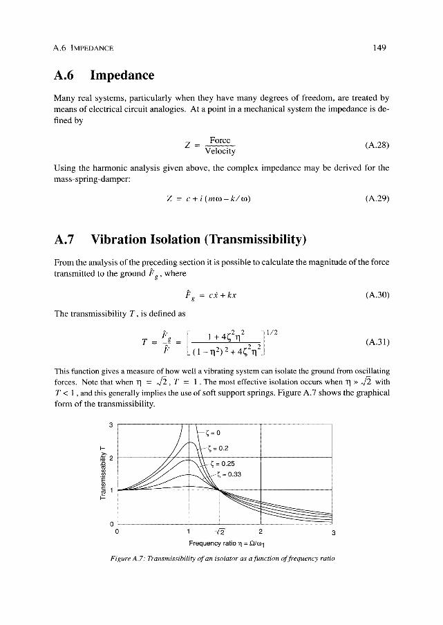
A.7 Vibration Isolation (Transmissibility)

From the analysis of the preceding section it is possible to calculate the magnitude of the force transmitted to the ground F g' where

The transmissibility T, is defined as

Fg T=

F

ci: + kx (A.30)

(A.3l)

This function gives a measure of how well a vibrating system can isolate the ground from oscillating forces. Note that when 11 = J2, T = 1. The most effective isolation occurs when 11 » J2 with T < 1 , and this generally implies the use of soft support springs. Figure A.7 shows the graphical form of the transmissibility.

3 ,------------..-.------------,-------------, I

I

~ 2 r----------/--7''---+--4+-----------+-

1

1

:g I gs ~ I

~ ----~I ____________ ~ ,::

2 3

Frequency ratio 11 ~ Q/w1

Figure A.7: Transmissibility of an isolator as afunction offrequency ratio

150 A BASIC VIBRATION THEORY AND ITS APLICATION TO BEAMS AND PLATES

The result is usually expressed in dB's of isolation according to the formula:

dB = 20· log (T) (A.32)

and this is shown in Figure A.8. It is apparent that damping does not have a strong influence for harmonic excitation though less damping is better. However, it can be shown that for tran­sient excitation (for example, machine start-up sequences) some damping is essential to pre­vent large motion as the system passes through resonance.:

A.8

0

\ 1

I I I ! I

, I I I I I

-10 \ I , I I

, I , I I ,

I i\ I I I I I: I I I I

-20 ~ I 'I ,: I I : I' ! I , I

1 ~i I! ! I I I I I' II

i I I ! 'i; I I I I I I I

-30

co .~ I I I

I I I

I I :l! I I I i I ! I I I ' ~ I

~ c -40 0 .~

"0 !!1

-50

: I : I ~ '" i

I I 1 I

I I I I I! 1\ ~1.;=0.1 I I I I I ! i: I

,

I I I I I \ I 1"'-. ~ I I

I ! I I I I , I ,

: :' I

! I i \: 'i 'h- J I I j I

-60 I i I! " i 1~ I

, I ! I !

i ~ I.; = 0.01 i I • I i I

-70

I

~ i : I

: : I , I ! : i : I 1.; = 0.001 ~ N , tl1iU--QI: I ,

I '--------l--80 1 2 5 10 20 50 100 200

Frequency ratio." = .Q/wl

Figure A.8: Attenuation in dB of the force transmitted to ground as a result afisolation

Continuous systems and their equivalent SDOF systems

In this final section we shall briefly consider the vibrations of beams and plates and how their fundamental vibration may be characterised as those of an equivalent single-degree-of-free­dam (SDOF) system. The basis of the analysis of real continuous systems is one of the fol­lowing:

(1) a continuum differential equation of motion for the system (2) a discrete finite element approximation, which can be more or less complex.

A.8 CONTINUOUS SYSTEMS AND THEIR EQUIVALENT SDOF SYSTEMS 151

In both cases the analysis can be reduced, by suitable coordinate transformations, to a problem involving a set of simple oscillators each of which describes one of the characteristic vibra­tions of the system. This is the basis of the normal mode method and the details of it can be found in good standard textbooks such as lA.I] and [A.2J. In certain circumstances only the fundamental mode of vibration is important and so the continuous system can be approximat­ed by an equivalent SDOF model. The circumstances in which this approximation works well are

(1) when the spatial distribution of forces is reasonably uniform (2) when the maximum frequency of the (Fourier transformed) force with non-negligible

force amplitude is less than or equal to the fundamental natural frequency, and (3) when the two lowest natural frequencies are not close in value.

In other circumstances consideration must be given to a more rigorous analysis involving the use of more modes of vibration, but this is beyond the scope of this appendix.

Equivalent SDOF systems can easily be found for beams and plates. The procedure for beams is shown in the following. For plates, the procedure is analogous.

To determine the properties of the equivalent SDOF we consider a beam of length L , stiffness EI and distributed mass Il. It is excited by a distributed load p' cos (Qt) .

Because we only consider the first eigenmode of the beam, the displacements can be ex­pressed simply as

w(x,t)= ~(t) ·f(x)

where w (x, t) displacement of the beam ~ (t) f (x)

displacement in a reference point at x = ~ shape of the first eigenform of the beam with f (x = ~) =

Using the Laplace equation

E.( 8Ek J _ 8Ek= 0 dtl8~ 8~

We find:

L L

~'IlJj2(x)dx + ~'E1J(f"(x))2dx o o

L

p' cos (Qt) J f (x) dx

o

(A.33)

(A.34)

(A.35)

Equation (A.35) can be written in the form of the governing differential equation of an SDOF system:

where in k

P

generalised mass generalised stiffness generalised load

(A.36)

152 A BASIC VIBRATION THEORY AND ITS APLICATION TO BEAMS AND PLATES

This equivalent SDOF has the same natural frequency as the original system, i.e. the beam, and the same reference displacement amplitude. The generalised properties of the equivalent SDOF can be found as follows. The generalised mass is given by:

L

/J- j P (x) dx == $ M . /J-L

o

where /J- distributed mass L length of the beam f shape of the first eigenform <I> M == mass factor

and

L

lJP (x) dx

o (A.37)

Obviously, the generalised mass is independent of the load. For a lumped mass the mass factor becomes f2 (x::: ~M) ,i.e. the square of the displacement of the first eigenform at the location of the lumped mass.

The generalised stiffness of the equivalent SDOF is given as

t L

k E/ f (f" (x)) 2dx = 1'} . ~; and ~3f (f" (x) ) 2dx o o

where EI flexural stiffness of the beam For certain materials the difference between the dynamic and static E -modules must be considered (see Appendix F for details).

1'} stiffness factor

For practical cases the generalised stiffness can be approximated as follows:

load factor (see below)

(A.38)

(A.39)

where <l>L k beam stiffness, i.e. stiffness at the reference point for the given load.

The generalised load is defined by the following equation

where <l>L p

L

P = pjf(x)dx=$t ·pL o

= load factor distributed load

and

L

lJf (x) dx o

The load factor for a single load acting at the reference point is always 1.0.

(AAO)

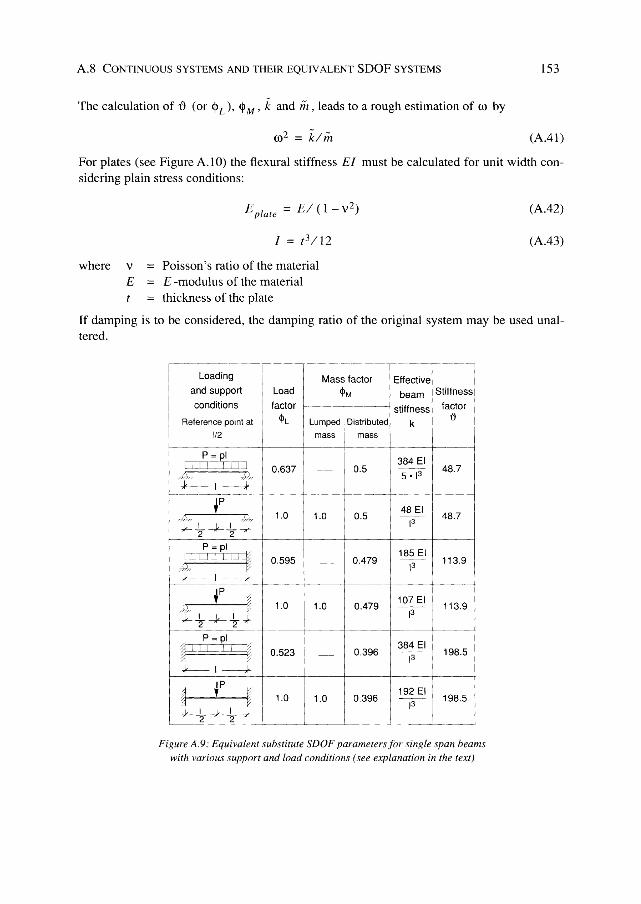
For simple cases of beams and plates the values of the load, stiffness and mass factor are given in Figures A.9 and A.I O. For systems or loads that are not shown there, the above described factors can easily be approximated using the static deflection curve instead of the first eigen­form of the system.

A.8 CONTINUOUS SYSTEMS AND THEIR EQUIVALENT SDOF SYSTEMS 153

The calculation of ~ (or <l> L)' <1> M' k and m, leads to a rough estimation of 0) by

(A.41)

For plates (see Figure A.lO) the flexural stiffness EI must be calculated for unit width con­sidering plain stress conditions:

where y

E

Eplate = EI (1 - y2)

I = t3 /12

Poisson's ratio of the material E -modulus of the material thickness of the plate

(A.42)

(A.43)

If damping is to be considered, the damping ratio of the original system may be used unal­tered.

---------- -i-------T- --,--, Loading I Mass factor I Effective! I

and s~pport Load I ~M : beam I Stiffness:

conditions factor I ; i stiffness! facto r 1

Reference point at <ilL i Lumped! Distributedl kit'} I I - ,

112 : mass : mass I

384 EI 48.7

P = pi: i

UlllIL::J I 0.637 I 05 ~~ ~;- I -- : -

~-I--~ I I f-~------IP-----l--- --------- -~-- --f----- --- -----

, I : ±~ I "l; "10 I 1.0 1.0 I 0.5 48.71 ~t~t~ i : r

p;;: pI I : ~ LLI--LD-L~ I 0.595 j_ : 0.479 1_8_~_E_1 113.9

I ';---I--,:c I I ~--- - - - - ----c'---+-----+--- ---I IP ,; I I I

107 EI

- --\-----j

I *)~ , ~ 1.0 1 1.0

i ~ t -*-+ ,(-+-----i----+----+_ _1

3_--+-__ --1

I ;:] I ri::i':c ~i

0.479 113.9

:r li 0.523 I I

0.396 384 EI

198.5

I -¥-- I ----+ I IP -'---+----+-----j----+----/ la , ') 192 EI

198.5 I ~t---'----it; 1.0 1.0 0.396 -13-

~ t+ + -~____' ___ ~ __ _'__ __ ___'_ ----.-L~ Figure A.9: Equivalent substitute SDOF parameters for single span beams

with various support and load conditions (see explanation in the text)

154 A BASIC VIBRATION THEORY AND ITS APLICATION TO BEAMS AND PLATES

I-­I

-

I Support conditions

I

I -------

'EjJ' , , I b I I a I

: ! -------

J:L a b 2

I~I .b.. a b 2

I a

-b

1.0

0.9

0.8

0.7

0.6

0.5

1.0

0.9

0.8

0.7

0.6

0.5

Load lactor

<PL

0.45

0.47

0.49

0.51

0.53

0.55

0.33

0.34

0.36

0.38

0.41

0.43

I

I I I I I

I

Mass I actor i I

<PM I

O.

O.

O.

O.

O.

I I

31 I

I I

33

35

37

39

Effective p'late

stiffness k

271 E10 ~

228EIO ~

212Elo --r

I O. 216Elo

~--! -2-1--T-870Elo :

41

r I i O. ~I

I O. 798Elo

23 I ~

O . 25

O. 27

O. 29

O. 31

Figure A.10. Approximate equivalent substitute SDOF parameters for rectangular plates with various support conditions (uniformly distributed mass and load only); the factors have been derived for simultaneous excitation

of more than one mode of vibration as a result of impact loading and are not true SDOF equivalents

B Decibel Scales H.G. Natke, G. Klein

B.I Sound pressure level

In acoustics, large numerical ranges of sound pressure are possible between minimum and maximum values. This makes their mathematical manipulation very cumbersome. Conse­quently, for acoustical purposes the unit of sound pressure was standardized to be the decibel [dB], which is defined as 20 times the logarithm of the ratio of the pressure to a suitable cor­responding reference pressure [ISO 131], [ISO/R 357], [DIN 45630/1].

If P is the sound pressure and Po the reference pressure, then the pressure level is given by

Lp = 20· logE. = 10· log( E.)2 = 10· 10g(f) [dB] Po Po 0

(B.l)

where I and 10 are intensities corresponding to p and Po' The reference sound pressure is defined by Po = 20 ~Pa = 2 . 10-5 N/m2 and is the r.m.s-value of the average human hearing threshold at 1000 Hz.

[dB] 10,; -0, -----,----,----1-----.1 ----,---~----~----~--~

o 1 [ I i

·10 I--t-I -----+-----t-I --~:,.L~_~--,i-----t---~------~--_+--____1

t 20 -- -7,/' i! . ~ ~:: t-/ 1 u_ - I i : I : i

:)( I I u~~i j~_~ _____ L _~~ 1.5 2 5 102 2 5 103 2 5 104 2

1 1 [

I [

[ , ........ ~ [ ,

[ [

I I 1 I

Frequency f [Hz]

Figure B.1: A-weighting

156 B DECIBEL SCALES

B.2 Weighting of the sound pressure level

In common use is also a weighting of the sound pressure level due to the perception charac­teristics of the ear, resulting in dB(A) values instead of dB values [DIN lEC 651]. The weight­ing is done by subtracting from the Lp [dB] value a value depending on the frequency and shown in Figure B.1. For example for 50 Hz a value of 30.2 dB must be subtracted from Lp [dB] in order to obtain the value in dB(A).

In the same way definitions can be used for other quantities such as intensities, and the r.m.s­values of accelerations, velocities and displacements. For example the displacement level is given by

Xrms Lx = 20 . log- [dB]

Xo (B.2)

with a reference value conveniently chosen as

Xo = 0.8· 10-11 m (B.3)

Concerning the velocity and acceleration levels the reference values are

Vo = 5.10-8 mls and ao = 5.10-4 m/s2 (BA)

The reference value va is given e.g. in [DIN 45630/1], the other reference values follow by conversion with 1000 Hz.

C Damping O. Mahrenholtz, H. Bachmann

C.I Introduction

Damping in a vibrating structure is associated with a dissipation of mechanical energy, usu­ally by conversion into thermal energy. The energy dissipation equals the work done by the damping force. In the case of a free vibration the presence of damping results in a continuous decay of the amplitude. In order to maintain a constant amplitude in the case of a forced vi­bration, the energy dissipation must be continuously replenished by an external mechanical energy source.

In Figure C. I the more important types of damping are shown.

C.2 Damping Quantities (Definitions, Interpretations)

In the case of oscillatory forcing functions, the stress (or the internal forces) are found to lead the strain (or the deformation). Thus a hysteresis loop is formed and completed during each cycle (Figure C.2)

The area

(C.l)

inside the hysteresis loop represents the mechanical energy dissipated, or the work done by the damping force, in a unit volume of the material.

The damping factor 'I' of the material is proportional to the ratio of energy dissipation W D

to maximum strain potential energy Epol (see Figure C.2b):

(C.2)

158

(J

£

Hysteresis (viscous, friction, perhaps yielding)

Relative motion between substructures (bearings, joints, etc.)

External contact ( non-structural elements, energy radiation to the soil, etc.)

Figure C.1: Different types of damping

a)

Figure C.2: Phase displacement and hysteresis loop

C DAMPING

£

The damping factor \f1 s of the structure is obtained by integrating over the volume of the structure and averaging:

\f1 s = f \f1 vdV = (C.3)

For a homogeneous structure is \f1 s = \f1.

If the structure is modelled as a simple linear oscillator with a harmonic forcing function (Figure C.3), the equation of motion is

mx+cx+kx = F(t) = FcosQt (CA)

where F is the amplitude and Q the circular frequency of the forcing function. A steady-state solution of Equation (CA) is

x = .¥cos(Qt-ljJ) (C.5)

The damping coefficient c represents viscous or linear damping.

C.2 DAMPING QUANTITIES (DEFINITIONS, INTERPRETATIONS) 159

For this case of linear viscous damping the energy dissipation in the structure, per cycle (of duration (period) T = 2n/Q), is then obtained as

T

W DS = f(c:i:):i:dt = ncQx2 (C.6)

o

The maximum strain energy in the structure is

E lk~2 potS = 2 x (C.7)

The damping factor Equation (C.3) becomes now

W DS cQ 'tjJs = _._- =

2n E potS k (C.S)

Frequently the damping is quite small and only affects the vibration behaviour significantly near resonance. For Q = WI = Jk/m (see Appendix A), the damping factor at resonance becomes

c

Jk;z (C.9)

The damping ratio S is also often used:

1; = _c_ = 2Ji;

(C.IO)

and it follows that

(C.ll)

The quantity 2mw1 is known as the critical damping coefficient ccril. Hence

1; = ...£ (C.12) ccrit

For c = ccrU (or 1; = 1) the vibration changes its time dependent character from an oscil­lating function to a function steadily converging to a zero displacement.

From Equations (C.8) and (C.ll) it follows that:

1 WDS 1; = 4n· ~

pOlS (C.13)

160 C DAMPING

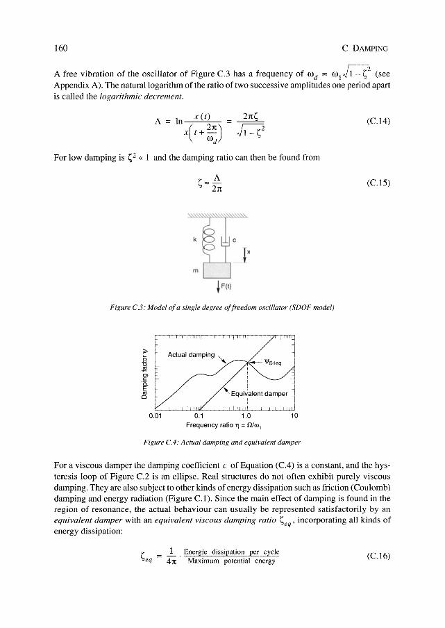
A free vibration of the oscillator of Figure C.3 has a frequency of Wd = WI n (see Appendix A). The natural logarithm ofthe ratio of two successive amplitudes one period apart is called the logarithmic decrement.

A=ln xCt)

x(t+ ~)

For low damping is 1;? « I and the damping ratio can then be found from

k

m

A ~"'-21t

Figure C.3: Model of a single degree offreedom oscillator (SDOF model)

Actual damping "

0.D1 0.1 1.0 10 Frequency ratio 11 = Q/w1

Figure C.4: Actual damping and equivalent damper

(C.14)

(C.1S)

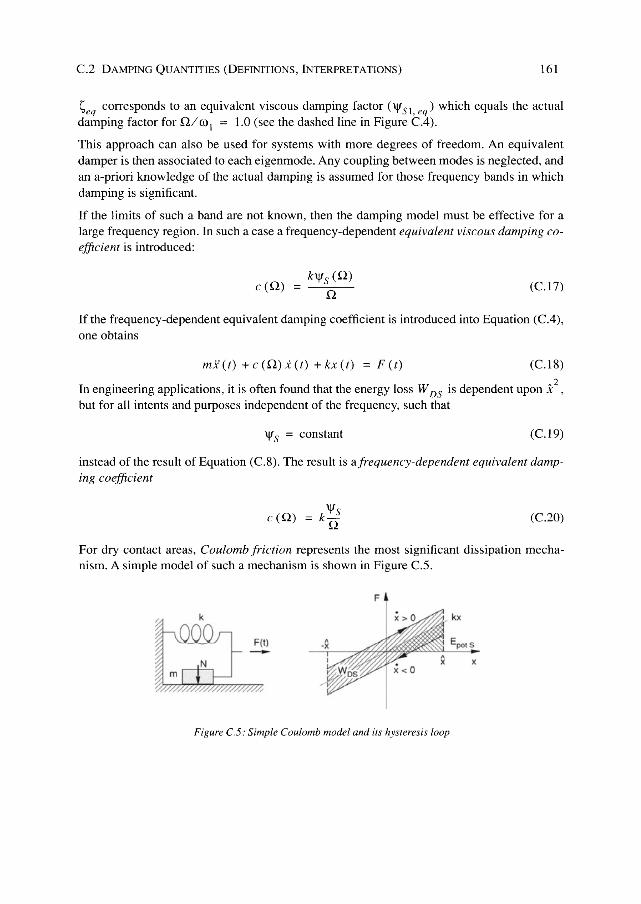
For a viscous damper the damping coefficient c of Equation (CA) is a constant, and the hys­teresis loop of Figure C.2 is an ellipse. Real structures do not often exhibit purely viscous damping. They are also subject to other kinds of energy dissipation such as friction (Coulomb) damping and energy radiation (Figure C.l). Since the main effect of damping is found in the region of resonance, the actual behaviour can usually be represented satisfactorily by an equivalent damper with an equivalent viscous damping ratio Seq' incorporating all kinds of energy dissipation:

~eq :::: 41t Energie dissipation per cycle

Maximum potential energy (C.16)

C.2 DAMPING QUANTITIES (DEFINITIONS, INTERPRETATIONS) 161

~eq corresponds to an equivalent viscous damping factor ('IIS1, eq) which equals the actual damping factor for Q/co] = 1.0 (see the dashed line in Figure CA).

This approach can also be used for systems with more degrees of freedom. An equivalent damper is then associated to each eigenmode. Any coupling between modes is neglected, and an a-priori knowledge of the actual damping is assumed for those frequency bands in which damping is significant.

If the limits of such a band are not known, then the damping model must be effective for a large frequency region. In such a case a frequency-dependent equivalent viscous damping co­efficient is introduced:

k'lls (0) c (0) = o (C.17)

If the frequency-dependent equivalent damping coefficient is introduced into Equation (CA), one obtains

mx(t) +c(Q)x(t) +kx(t) = F(t) (e.IS)

In engineering applications, it is often found that the energy loss W DS is dependent upon i 2 ,

but for all intents and purposes independent of the frequency, such that

'lis = constant Ce.19)

instead of the result of Equation (e.S). The result is afrequency-dependent equivalent damp­ing coefficient

(C.20)

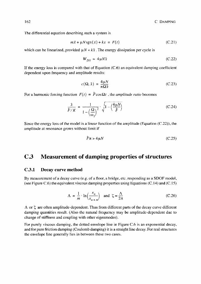
For dry contact areas, Coulomb friction represents the most significant dissipation mecha­nism. A simple model of such a mechanism is shown in Figure C.S.

F

kx

F(!) EpolS - x m

Figure C.5: Simple Coulomb model and its hysteresis loop

162 C DAMPING

The differential equation describing such a system is

mx + !ANsgn(X) + kx = F(t) (C.2l)

which can be linearized, provided !AN « k'X . The energy dissipation per cycle is

(C.22)

If the energy loss is compared with that of Equation (C.6) an equivalent damping coefficient dependent upon frequency and amplitude results:

( r"I ~) _ 4"",N c ~~, x - r"I~ :n:.~x

For a harmonic forcing function F(t) = Fcos Qt , the amplitude ratio becomes

(C.23)

(C.24)

Since the energy loss of the model is a linear function of the amplitude (Equation (C.22», the amplitude at resonance grows without limit if

(C.2S)

C.3 Measurement of damping properties of structures

C.3.1 Decay curve method

By measurement of a decay curve (e.g. of a floor, a bridge, etc. responding as a SDOF model, (see Figure C.6) the equivalent viscous damping properties using Equations (C.14) and (C.IS)

1 (Xn) A A = -' In -- and 1; "'" -m xn+m 2:n:

(C.26)

A or 1; are often amplitude-dependent. Thus from different parts of the decay curve different damping quantities result. (Also the natural frequency may be amplitude-dependent due to change of stiffness and coupling with other eigenmodes).

For purely viscous damping, the dotted envelope line in Figure C.6 is an exponential decay, and for pure friction damping (Coulomb damping) it is a straight line decay. For real structures the envelope line generally lies in between these two cases.

C.3 MEASUREMENT OF DAMPING PROPERTIES OF STRUCTURES 163

C.3.2 Bandwidth method

For an ideal damper and small damping (~« 1 or ~ < 0.1, respectively), the damping ratio can be obtained from the half power bandwidth (Q2 ~ QJ ) (Figure C.7) from the resonance curve due to a harmonic forcing function [C.l]:

(C.27)

Instead of the displacement amplitude curve the velocity or the acceleration amplitude curves may be used but only, of course, in cases where damping is low.

However, for measurement of damping in most cases the bandwidth method cannot be rec­ommended. Non-linear behaviour of the structure may lead to a turning of the peak of the res-

x

Figure C.6: Measured decay curve

A I xmax I ~~---------- ----",2 I I I

I

I ~ I

I

0 1

half-power bandwidth

-t

o

Figure C.7: Resonance curve with ha!fpower bandwidth

164 C DAMPING

onance curve to the left (increasing stiffness with displacement) or to the right (decreasing stiffness with displacement), with the result that for a certain value of Q/w) two (or three) different amplitudes may occur. This makes it very difficult to evaluate the resonance curve. Also measuring errors will affect to a great extent the determination of the damping quantity. In addition, the effort expended in measuring a resonance curve is much higher than that for the measurement of a decay curve.

C.3.3 Conclusions

In most practical cases damping is evaluated by the decay curve method rather than by the bandwidth method. In practice a more or less free decay can be produced by one of several methods, for example: by people standing still after jumping at the resonance frequency, or by abruptly stopping a rotating eccentric type of machine, or by imparting an impact such as a dropped sandbag (provided that one natural frequency dominates the vibrational behaviour). For horizontally vibrating structures (and in some cases for vertically vibrating structures al­so) an initial displacement may be produced by the sudden release of a steel cable or using the pulse of a rocket.

C.4 Damping mechanisms in reinforced concrete

Material damping in reinforced concrete elements (and similarly in partially prestressed con­crete elements) in the quasi-elastic range (no yielding of reinforcement) shows some special features mainly due to cracking. The damping depends strongly on the stress intensity. Figure C.S shows the equivalent damping ratio S of a bending element or a beam mainly sub­jected to bending moments. The stress intensity may be characterised by the stress amplitude in the bending reinforcement or by the displacement amplitude of a beam, both defined at the point of maximum stress or displacement respectively.

For low stress intensity. corresponding to the uncracked state, relatively low damping ratio (s < I %) exists. With formation of cracks the damping ratio increases. In the final cracked state but still with relatively low stress intensity the damping ratio is relatively high, perhaps twice or three times the value of the initial uncraeked state. With further increase in the stress intensity the damping ratio decreases rapidly and may reach a value smaller than that of the initial uncracked state.

This damping behaviour can be explained as follows [C.2]:

• In the un cracked state nearly pure viscous damping occurs in the concrete. • In the cracked state two kinds of damping occur:

- nearly pure viscous damping in the concrete in the uncracked compression zone - nearly pure friction damping due to friction between the concrete and the reinforcing

steel in the cracked tension zone.

Figure C.9 shows a cracked bending clement and a corresponding relevant model. The damp­ing in the compression zone is modelled by a viscous damper, and the damping in the tension

C.4 DAMPING MECHANISMS IN REINFORCED CONCRETE 165

zone by a friction damper. The spring represents the bending stiffness of the bending element, and m represents the relevant mass.

Following the definition of the equivalent damping ratio according to Equation (C.16) one can see: E potS is proportional to the square of the stress intensity, in Equation (C.7) represented by x. The energy dissipation per cycle due to viscous damping, W DS ' is also proportional to the square of the stress intensity, see Equation (C.6). Hence for constant depth of the bending compression zone a viscous damping component of S results which is independent of the stress intensity. On the other hand, the energy dissipation per cycle due to friction damping, W DS' is linearly proportional to the stress intensity, see Equation (C.22) . Hence a friction damping component of S results which decreases hyperbolically with increasing stress inten­sity.

Note that with increasing stress intensity the energy dissipation per cycle, in spite of the de­creasing equivalent damping ratio S, is increasing due to the fact that the maximum strain en­ergy E potS is increasing.

Viscous damping I in un· ' cracked state

\ \ __ - After cracking \ \

1

~1 \ [I I Friction \ damping ll' -_---i~~.:':.a.::~:.'!..:.t~~-------V'SCOUS damping

in cracked state _ 1_ - ..L - --- - - - - - -­

-------. Stress intensity I Fully cracked state

: ,-Formation of cracks -Uncracked state

Figure C.S: Equivalent damping ratio of a reinforced concrete element in different states [C.2]

Bending element

M

~ Crack distance ...

l Viscous ( damping

> Friction damping

Model

Reinforcement surface

Figure C.9: Cracked bending element and relevant model for material damping of reinforced concrete [C.2]

166 C DAMPING

CoS Overall damping of a structure

Depending on the location of energy dissipation the total overall damping of a structure (e.g. a bridge, a gymnasium, a tower, etc.) is a sum of the following contributions:

- damping of the bare structure - damping by non-structural elements - "damping" by energy radiation to the soil

While the first contribution always exists, the second and/or the third contribution may be great or small or not present depending on the type and purpose of the structure.

C.S.1 Damping of the bare structure

Energy dissipation in the bare structure occurs by

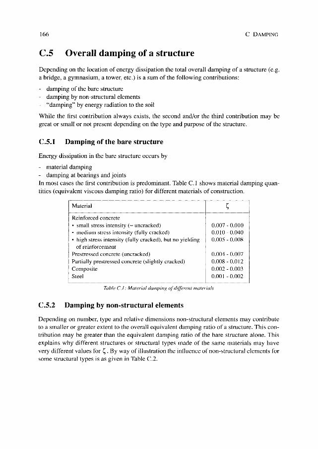
- material damping - damping at bearings and joints In most cases the first contribution is predominant. Table C.l shows material damping quan­tities (equivalent viscous damping ratio) for different materials of construction.

Material

Reinforced concrete o small stress intensity (- uncracked) o medium stress intensity (fully cracked) o high stress intensity (fully cracked). but no yielding

of reinforcement Prestressed concrete (uncracked) Partially prestressed concrete (slightly cracked) Composite Steel

0.007 - 0.010 0.010 - 0.040 0.005 - 0.008

0.004 - (l.{)07

0.008 - 0.012 0.002 - 0.003 0.001 - 0.002

TaMe c.J: Material damping of different materials

C.S.2 Damping by non-structural elements

Depending on number, type and relative dimensions non-structural elements may contribute to a smaller or greater extent to the overall equivalent damping ratio of a structure. This con­tribution may be greater than the equivalent damping ratio of the bare structure alone. This explains why different structures or structural types made of the same materials may have very different values for s. By way of illustration the influence of non-structural elements for some structural types is as given in Table C.2.

C.S OVERALL DAMPING OF A STRUCTURE

Type of structure

Footbridges (vertical excitation)

Non-structural elements

• pavement • railings

Influence of non-structural clements

I i in general relati vel y small i I

167

- - ------------- -- --+-------- - -- - - ------------j-- --- - ----- ---- ----

Gymnasia (vertical excitation)

Building floors (vertical excitation)

Towers (horizontal wind excitation)

• flooring in general moderate • fa~ades • equipment

• partition walls in general relatively great • flooring • furniture • ceilings • mechanical services

• equipment in general small • mechanical services

Tahle C.2: Influence a/non-structural elements 011 overall damping

C.S.3 Damping by energy radiation to the soil

Energy radiation to the soil by travelling waves may also contribute significantly to the overall equivalent damping ratio. By way of illustration the influence of energy radiation for some structural types is as given in Table C.3

1 Type of structure

I 1

I 1

I

Footbridges (vertical excitation)

Bearings/Supports/Soil Influence of energy radiation

1 • steel bearings supporting a small beam structure

• vibrating support structures I medium to great (columns or walls) have direct contact with the earth

,-- - - - - - __ - __ - __ - - - ________ - - - __ - - _____ --1- ______________ _

i Towers • medium stiff or soft soil : medium to high I I ~

(horizontal wind excitation) • stiff sailor rock I low

Tahle C.3: Influence of energy radiation on overall damping

C.S.4 Overall damping

The great differences which are possible for the damping of the bare structure (predominantly material damping). for the damping by non-structural elements and for the damping by energy radiation to the soil, explain why very different damping quantities may result

- for different materials of construction - for different structure types, although they are of the same material of construction - for different structures of the same material of construction and the same structure type.

168 C DAMPING

Consequently the damping quantitites given in the different sub-chapters of this book cover a relative wide range.

In the case of a real vibration problem, where I;; cannot be measured, it is the task of the struc­tural engineer to take into account the influences described above in making a cautious assess­ment or estimate of the overall equivalent viscous damping ratio.

For reinforced concrete structures subjected to wind, damping quantities are given in Appendix H. Note that the subdivision of the overall damping quantity is different from that described above at the beginning of Appendix c.s.

D Tuned vibration absorbers H. Bachmann. H.G. Natke

D.I Definition

A vibration absorber is a vibratory subsystem attached to a larger primary vibration system. The vibration absorber consists in general of a mass, a spring and a damper (or some parallel springs and dampers). Accurate tuning of the frequency of the absorber results in induced inertia forces of the absorber mass which counteract the forces applied to the primary system, and less work is done on this system. Hence, the normal practical function of the absorber is to reduce resonant oscillations of the primary system (even though in theory it could be used as an inertia balancer at any frequency, provided it is tuned with respect to the forcing fre­quency). While the vibration amplitudes of the primary system can thus be suppressed to a large extent, large displacement amplitudes must be accepted in the absorber system [D.lJ, [D.6], [D.?], [D.8].

D.2 Modelling and differential equations of motion

In most cases vibration at one natural frequency of the primary system is troublesome and requires attenuation. This system can then be modelled as an equivalent single degree of free­dom system (SDOF-system, see also Appendix A). Together with the absorber system a two degree of freedom system results (see Figure D.I). The relevant equations of motion are:

where s

x

m c k Fcos(Qt)

=

= =

parameter subscript for the primary system parameter subscript for the tuned vibration absorber total displacement mass damping coefficient (see Appendix C) spring constant harmonic excitation (see Appendix A) of the primary system

(D.I)

(D.2)

170 D TUNED VIBRATION ABSORBERS

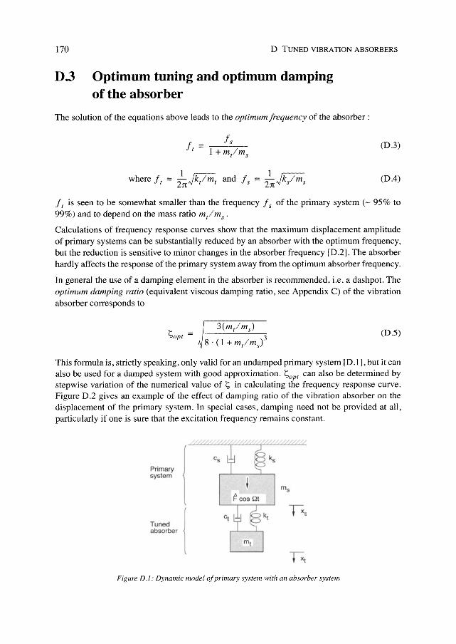
D.3 Optimum tuning and optimum damping of the absorber

The solution of the equations above leads to the optimum frequency of the absorber:

where it = 2lJtJk/mt and is = 21JtJk/ms

(D.3)

(D.4)

it is seen to be somewhat smaller than the frequency is of the primary system (- 95% to 99%) and to depend on the mass ratio mr/ms.

Calculations of frequency response curves show that the maximum displacement amplitude of primary systems can be substantially reduced by an absorber with the optimum frequency, but the reduction is sensitive to minor changes in the absorber frequency [D.2]. The absorber hardly affects the response of the primary system away from the optimum absorber frequency.

In general the use of a damping element in the absorber is recommended, i.e. a dashpot. The optimum damping ratio (equivalent viscous damping ratio, see Appendix C) of the vibration absorber corresponds to

(D.5)

This formula is, strictly speaking, only valid for an undamped primary system [D.l], but it can also be used for a damped system with good approximation. Sopt can also be determined by stepwise variation of the numerical value of S in calculating the frequency response curve. Figure D.2 gives an example of the effect of damping ratio of the vibration absorber on the displacement of the primary system. In special cases, damping need not be provided at all, particularly if one is sure that the excitation frequency remains constant.

Primary system

Tuned J absorber 1

~ cos Qt

Figure D.l: Dynamic model of primary system with an absorber system

D.4 PRACTICAL HINTS 171

The effectiveness of the absorber is less affected by a difference between the actual damping and the optimum damping of the absorber than by a difference between the optimum frequen­cy and the actual frequency of it. Hence poor tuning of the absorber after installation or de­tuning over time caused by changes in the stiffness of the primary system or of the absorber springs or by changes in masses may strongly reduce the effectiveness of the absorber.

11) C\I

0 C\I

0 t) J'1 11)-

c 0

~ ()

"" 'c 0-Ol co :2

11)-

/ xs.stat

0

0 1.5 3.0

I II II II :\-___ - Without tuned II absorber II II II 1\ I I I I I \ I \ I I I I I

: \--s~3%

---~~15%

-- ~opt ~ 9.1 %

4.5 6.0 7.5 Frequency [Hz]

9.0

Figure D.2: Example of the efj(!ct of the damping ratio ~ of the vibration absorber on the frequency response of a primary system

D.4 Practical hints

To examine a possible application of a tuned vibration absorber and to design such a subsys­tem, the following factors must be considered:

- The application of vibration absorbers can be considered whenever critical dynamic forc­ing cannot be avoided, especially in cases where existing or planned structures are difficult to stiffen economically.

- Experience shows that the application of vibration absorbers can be a good solution in the case of one-dimensional beamlike structures such as footbridges, chimneys and pylons of cable stayed bridges, whereas in cases of two-dimensional plate-like structures, such as gymnasium floors, dance floors and concert hall floors, an array of absorbers is needed which is not always an economical solution.

- A vibration absorber of the type described above is only effective over a narrow frequency band and when tuned to a particular structural frequency. It does not work satisfactorily for primary system structures with several closely spaced natural frequencies which are all more or less excited by the dynamic action in question.

172 o TUNED VIBRATION ABSORBERS

- A vihration absorber is more effective · the larger the mass of the absorber compared with the (modal) mass of the primary sys-

tem (due to the limitation of the displacement amplitude of the absorber mass), and · the smaller the damping of the primary system is. Absorbers are particularly well suited for reducing resonant vibrations of structures of not too large a mass and small inherent damping; they will prove inadequate for structures with a large mass or strong vibration despite substantial inherent damping.

- Depcnding on the mass and the damping of the primary system and on the required reduc­tion of the amplitudes of this system, for a first design approach the mass ratio m / m s may be chosen in the range of 1/15 to 1/50. The influence of this parameter should be studied. Beyond a certain absorber mass any further increase in mass results only in negligible fur­ther reduction of the vibration amplitudes of the primary system.

- The dynamic displacement amplitudes of the absorber mass has to be checked by calcula­tion.

- The fatigue behaviour of the absorber springs must be considered. - Design and installation of an absorber have to take into account

· a possible need to replace springs and dampers at some later date · the prevention of the absorber mass from falling down in the case of a spring failure.

- In many cases compression springs are more suitable than tension springs. - Theoretical calculation for the primary system and the absorber is not sufficient on its own

for determining the final absorber parameters. Rather, the accurate frequency of the prima­ry structure has to be measured in situ, and the absorber design should allow for refined tuning after installation. This is more easily done by altering the absorber mass than by var­ying the spring properties.

Examples of the application of tuned vibration absorbers are given in [0.3], [DA], [0.5].

E Wave Propagation G. Klein, l.H. Rainer

E.I Introduction

The propagation of waves plays an important part in vibration control, particularly when housing and other sensitive installations are to be planned for minimal vibration effects. Such an evaluation will inevitably entail measurements since the ground is a very irregular trans­mission medium and consequently difficult to treat analytically. With the following theoreti­cal treatment of wave propagation in idealized media, however, an approximate evaluation can be carried out. Further details on this topic can be found, for example, in [E.l] and [E.2].

E.2 Wave types and propagation velocities

An elastic, homogeneous and isotropic medium with density p is characterized by the elastic constants of modulus of elasticity E and Poisson's ratio v, from which the shear modulus G = E/2 (I + v) can be derived.

Alternatively, Lame's constants A = vEl (1 + v) (1 - 2v) and 11 = G can be used.

In an infinite continuum, two types of waves exist whose propagation velocities are

/(1.+211) - J E(I-v) Ai p - p(l +v) (l-2v)

v = JI1/p = J E = JG/p s 2p (1 + v)

(E.I)

(E.2)

The first is called a P-wave (or compression wave, primary wave, longitudinal wave), for which the particles of the ground vibrate parallel to the direction of wave propagation. The second wave is called S-wave (or shear wave, torsional wave, secondary wave, transverse wave), for which the particles vibrate perpendicular to the direction of wave propagation. From the ratio v pi v s = J2 (I - v) 1(1 - 2v) > 1 it can be seen that v p is always greater than v 5' and thus at a measurement point, the longitudinal wave will always arrive before the transverse wave.

174 E WAVE PROPAGATION

5 , I ,

J I I , I ,

,

!---- ---- - Ip~) I -:-r ,

S-wave

4

3

2

I R-wavi I

00 0.1 0.2 0.3 0.4 0.5

Poisson's ratio v

Figure E.1: Relation between Poisson's ratio and velocities of propagation

-0.6 -0.4 -0.2

Amplitude in depth z Amplitude of surface

0.0 0.2 0.4 0.6 0.8 ,

1.0 1.2 0.0 , , Horizontal L : ~ Ff--j t component T ....-0 ::::;;;; ..- l , \ 0.2 [U(zl] 7; ~ i : // VV , ,

I I !(( 1(1 , ,

/# VI , , , I ,

i H It ( , v:>::::-rA I, , Vertical 1 I 1\\ ,\ \ I I

, V,::-t:/":/ 'component I I I ~\\1 I I K V,V I ~[V(z)] 1

j

--1 I \\\\ , i v''/ V'hU = 0.25 I I ' ..J. V = 0.25 )i~ I 'I. y'£V' !'-v = 0.30 '

,

fV = 0.30, /\\1 I 'f Ii ~ V = 0.40 I ' I I 11 fV = 0.40 if/l;!-~ u = 0.50 I ,

f"~o,50jr ' , I "j I 'I I I jj I I , 111'1 : I-t-l-r-L ,I f(f ~ . i-t-+--- -r- ,-- '-

I -'-, '1

~~_l_J __ U J//lL ,I LJ ,

0.4

0.6

0.8

.0

.2

.4

Propagation

C Particie motion

" Particle umotion

Figure E.2: Relation between amplitude ratio and dimensionless depth for Rayleigh waves with v as parameter

In a perfectly elastic halfspace, a third type of wave is fanned, the R-wave (Rayleigh wave), whose propagation velocity vR can be obtained from Figure E.1. As an approximation:

Vs (0.86 + 1.l4v) vR "" l+v

(E.3)

Figure E.2 shows the variation of the vertical and horizontal component of the Rayleigh wave as a function of depth z and the Poisson's ratio v . Both components decrease sharply with depth. At a depth equal to one wave-length A, i.e. z == A. the vertical component is reduced by about 70%, the horizontal component by about 85%. This is therefore a surface wave. The

E.3 ATTENUATION LAWS 175

Granite, Basalt

Sandstone, Limestone

Broken stone

Gravel

Sand, dry -Sand, weI

Sand, saturated ~ Clay, loam

Water 11srm/s Air 1330 mls

o 2000 4000 6000

Wave velocity vp [m/s)

Figure E3: Typical velocities oj compression waves (P-waves}for rocks and soils

vertical component vibrates always in phase, whereas the horizontal component has a phase reversal at about z = 0.2A as a result of which the direction of the elliptical particle motion is reversed. Waves with low frequency components, as is the case with earthquakes, have rel­atively long wave-lengths. They therefore affect the earth's surface to a greater depth than high frequency waves with relatively smaller wave-lengths. The latter would be likely to originate from machine foundations . Typical recommended values for propagation velocities are pre­sented in Figure E.3. Poisson's ratio for cohesionless loose soils can be taken as 0.3.

The propagation of vibrations in the ground is characterized by a decrease in vibration ampli­tudes with distance. Particle velocity is generally used as the appropriate measurement quan­tity. The attenuation depends on the type of the vibration source as well as the type of wave generated. The intensity of particle velocity is further reduced on account of geometric dis­persion; another reduction is due to material damping of the soil.

E.3 Attenuation laws

An attenuation law is given by

v = (Ri)n'D Vi R

(EA)

where V = vibration amplitude at distance R Vi vibration amplitude at reference distance Ri n = exponent of the amplitud reduction law D factor taking account of the transmitting medium

The exponent n for amplitude reduction depends on

- the geometry of the vibration source (point source, line source) - the type of excitation (stationary, impulsive) - the predominant type of wave (Rayleigh waves on the surface, body waves at some depth).

l76 E WAVE PROPAGATION

For point sources (e.g. machine foundations) the value of n is n = 0.5 for surface waves from stationary excitations and n = 1.0 for impulsive sources. For body waves the corresponding values are n = l.0 and l.5.

For line sources (e.g. traffic) the values are n = 0.0 and 0.5 for surface waves and n = 0.5 and 1.0 for body waves.

The material term D is given by D = exp ( [-u (R - R i)] ) , with the attenuation coefficient u "" 21t~/A : A is the wave length, ~ is the damping ratio of the transmitting medium. For loose soils ~ "" 0.01 can be used.

Since the attenuation in amplitude can extend over many powers of 10, the measure of atten­uation is often given in decibels [dB], which is defined as dB = 20 . log (Q / Q 1) . Q i is a fixed reference amplitude, specifically a particle velocity of 5 xl 0-8 Mis. The measured amplitudes (at the source or at any point in the medium) are then referred to this reference quantity. Thus one obtains two dB-values whose difference is a measure of the attenuation of the vibration amplitudes between the two particular measurement points (see also Appendix B).

F Behaviour of concrete and steel under dynamic actions W. Ammann, H. Nussbaumer

F.l Introduction

Under dynamic actions most material properties - such as modulus of elasticity, strength and strain limits - change to a greater or lesser extent, when compared with the corresponding val­ues for slow, quasi-static loading. The change is usually expressed as a function of the strain rate and in some cases also as a function of the stress rate or the rate of loading. The strain rate is defined as

d£ dt

and expresses the variation of strain with time. The stress rate is defined as

. da a == -dt

(F.l )

(F.2)

In most vibration problems the average strain rate seldom exceeds £ == 0.1 S-l so that expected changes in material properties are only moderate. A much larger effect occurs for strain rates t == 1 to 10 S-I as is typical of high impact forces. Dynamic actions may also influence the fatigue resistance of the structural material, even at a low number of cycles if the forces are large enough (low-cycle fatigue).

The following survey is mainly restricted to plain concrete with normal weight natural aggre­gates and to reinforcing steel. This survey is in accordance with a relevant chapter in [F.l]. It is not the aim of this survey to reproduce all literature data nor to give physical explanations for the relations established. Therefore this survey is not directed to materials specialists, but rather intended for structural engineers who are faced with impact problems. This appendix presents todays knowledge of materials in a condensed practical form. It allows stress or strain rates to be taken into account by means of graphs or simple empirical formulae. The changes of material property are usually described by a straight line when plotted against the strain rate on a semi-logarithmic scale and are therefore defined by an empirical factor with respect to the quasi-static value (i.e. £ = 5· 10-5 sol).

178 F BEHAVIOUR OF CONCRETE AND STEEL UNDER DYNAMIC ACTIONS

The changes of material properties under the influence of dynamic actions must be considered in relation to the reliability of other values used for the calculation, such as soil properties, etc. The aging of concrete, i.e. the increase of the material properties with time is generally ne­glected and design values are defined at an age of 28 days.

For practical calculations (e.g. of the natural frequencies of R.C. towers or pedestals of ma­chines) the increase in the Young's Modulus under dynamic loads may be neglected and the corresponding value at quasi-static loading to be used.

fdyn

4 ~~~m~t ______________________ ~~~~T 4

3 -

2.5

2 -1.8 1.6 1.5 1.4 1.3 1.2 1.1 -1

Compression

0.9 ,f-----,----.-----.---,---,--------,----,---i 0.1 la' 102 103 10'

3.10.5

I I i I I i

10-5 10-4 10-3 10'2 0.1

105 106 107 108

cr [N/mm2s] I I p

10 102 103

E [5']

3

2.5

2

1.5

Figure FI: Influence of stress and strain rate on concrete properties in compression [F.] J

fdyn

4T.;;;;-

I Tension

~ Eu,dyn

Esta! ' Eu,stat

3 -

:.5~, 1.8 1.6 1.5 1.4 1.3 1.2 1.1 1 0.9

~1 1~ 1~ 1~ 1~ 1~ 1~ 1~ 1~ 3.10.5 cr [N/mm2s]

I I I I I I I i I

10-5 10-4 10-3 10-2 0.1 10 102 103

E [5"]

4

Figure F2: Influence of stress and strain rate on concrete properties in tension [F.IJ

F.2 BEHAVIOUR OF CONCRETE 179

F.2 Behaviour of concrete

F.2.1 Modulus of elasticity

The modulus of elasticity (Young's Modulus) of concrete in compression increases with stress and strain rate as

E IE = (crl cr ) O.Q2S with cr = I N/mm2s or dyn slat 0 0 (E3)

E IE = (Ut) 0.026 with t = 30 . 10-6 S-l ~n s~ 0 0

(F.4)

These relations are supposed to be valid for all grades of concrete. Figure EI shows the ratio between dynamic and static modulus of elasticity as a function of stress and strain rate.

The influence of stress rate on the modulus of elasticity in tension is smaller than for compres­sion. The graph of Figure E2 can be formulated as

E dynl E stat = (crl cr) 0.016 with cr 0 = 0.1 N/mm2s or CES)

(E6)

These relations are valid for all stress and strain rates and all concrete grades. In most cases of dynamic action (but not impact) the increase in modulus of elasticity due to the strain rate effect does not exceed 20%.

F.2.2 Compressive strength

The compressive strength of concrete can be written in terms of strain rate as

f If = (£It) 1.026a with 0. = I for £ < 30 sol dyn stat 0 5 + 3/,m14 - (E7)

where lern = mean static cube strength of concrete [N/mm2].

This relation reveals the fact that the influence of loading rate decreases as the grade of con­crete increases. The formula accounts also for the influence of the strain rate on the modulus of elasticity. If the influence of the strain rate on the modulus is not considered the power of the equation above would be 1.0 0. . Figure EI shows the influence of stress and strain rate on the ratio of dynamic to static compressive strength. Beyond a strain rate of 30 S-l the increase is very pronounced.

F.2.3 Ultimate strain in compression

The ultimate strain £u is the strain which occurs at maximum stress. The ultimate strain as a function of strain rate is (see Figure EI):

£u,dy/£u.stat = (tl£o) 0.020 with to = 30.10-6 s'! (see Figure EI). (E8)

180 F BEHAVIOUR OF CONCRETE AND STEEL UNDER DYNAMIC ACTIONS

F.2.4 Tensile strength

In contrast to compressive failure, tensile failure is always a discrete phenomenon. Usually one crack occurs which divides a specimen into two parts. The two separating parts are un­loading while the crack width increases. Energy consumption occurs in the cracking zone. The formulation is similar to compressive strength except for the value of the coefficient.

Taking account again of the influence of strain rate on Young's modulus a relation can be de­fined between strain rate and tensile strength as follows (see Figure F2):

f If = (£Ie) l.0160 with 0 = 1 for e s 30 sol dyn sIal 0 10 + f 12 '

em (F9)

where fern = mean static cube strength of concrete.

Tensile strength is more sensitive to strain or stress rate if the concrete has a low grade and is more sensitive to strain rate than compressive strength.

Usually compressive strength is the reference value for the concrete grade and is therefore known. The tensile strength can be estimated from

(FlO)

which is a CEB-FIP recommendation for mean values of concrete strength.

F.2.S Ultimate strain in tension

Ultimate strain IOu is the strain at maximum stress and can be expressed as a function of strain rate with (see Figure F2):

(Ell )

This relation is recommended for all stress and strain rates as well as all concrete grades.

2.4 I------j----j----i----t---i-

~:~~ 1.8 1----+--

1.6 ,L---+---j----i-r~--t--

1.4 ~--1.2 r---t-.7'~:o-+-~=-t-=

1.0 --

10' 102 103 10'

a)

'dyn I 'stat 2·°1-- ------,----.--

I 1.8 f-----+---+-----j---+--+---+i , 1.6 f--- ,

1.4 :-, -- ---t-1.2 ~--- ----,' :;;o-~-,

1.0 [: ::J~E~==~~~ 1

b)

10' 103 10'

Figure F3: Influence of stress rate on bond properties iF2l a) at a relative displacement of 8 = 0.01 mm b) at a relative displacement of 8 = 0.2 mm

F.3 BEHAVIOUR OF REINFORCING STEEL 181

F.2.6 Bond between reinforcing steel and concrete

The influence of stress rate on the bond of smooth bars and strands is negligible whereas the influence on the bond of defonned bars is considerable. It depends on concrete quality and relative displacement (slip) between steel and concrete. For the bond stress the following for­mulation is valid:

0.7· (1-2.58)/f~;;; relative displacement [mm] mean cube strength [N/mm2] 0.1 N/mm2

This relation is valid under the following conditions:

0< 0 < 0.2 mm (see Figure F.3) and 0.065 < AR/ A{) < 0.1

rib area cross section area of rebar relative rib area

F.3 Behaviour of reinforcing steel

(F.12)

(F.13)

The influence of strain rate on steel properties can be expressed by the following generalized relationship:

where Sdyn

S stat £

strength or strain value at elevated strain rate strength or strain value at quasi-static condition (so)

strain rate strain rate at quasi-static condition (£0 = 5 . 10.5 S·l)

regression coefficient

(F.14)

This linear approach is used for the sake of simplicity although the standard deviation of the test results is often rather large and regression lines of second or third order would provide a better fit with data.

F.3.1 Modulus of elasticity

The modulus of elasticity (Young's Modulus) remains unchanged with

E = 2.06· lD-'N/mm2 (F.15)

182 F BEHAVIOUR OF CONCRETE AND STEEL UNDER DYNAMIC ACTIONS

F.3.2 Strength in tension

The formulas (valid for for f ~ 10 sol) for strength in tension are all of the form:

f/l", = l+K·ln(Ufo )

where fs

l", K

dynamic material properties with strain rate t [N/mm2] quasi-static material properties with strain rate to [N/mm2] coefficient taking account of steel and strength type (see Table F.l)

A set of measured data for hot rolled steel is given in Figure FA

K

Steel type yield stress proportional tensile strength ultimate limit strength

fs/fsyo f sO.21 f sO.20 fs/fsto fs/ f sro

Hot rolled steel 6.0lfsyo - 7.0lfsto 1.51 f sro Tempcore steel 5. lI f syo - 6.41 fsro -Cold worked steel - 4.31 f sO.20 6.51 f sto 1.91 fsro Mild steel *) 12.01 fsyo - - -

High quality steel**) - - - -Prestressing wires **) - - - -

(F.16)

*) Only very limited data available. Strength increase is more pronounced than for hot rolled steel **) Practically no influence of strain-rate

Table Fl: Coefficients for the calculation of strain-rate dependent strength in tension of steel

700

650

'" E

! 600

CfJ en ~ (jj 550 '0 a; >=

500

I i

I ! I I I I i I I I I I I

I I I i I I I I i I I I ! , I I

g

I I I I

I I !

~ ~ I I i :i I I 0 I I

f-~ I I i I I ,=

o '" I ~ ~ ~::;...-- T' I~ fi c£. ~t-~ ; ~ n+ -!tt-~ t-~ l- .-

I+; ~ c::"-

I 8 I i I !

I "'"

I I I i I I I

I I I I

I I I

I I I fil

I I I I

I I I

450 10-5 10-4 10-3 10-2 10-1

Strain rate [1 Is]

Figure F4: Influence of strain rate on yield stress of hot rolled reinforcing steel [F3j. the regression lines indicate some minor influence of the different bar diameters

F .3 BEHAVIOUR OF REINFORCING STEEL

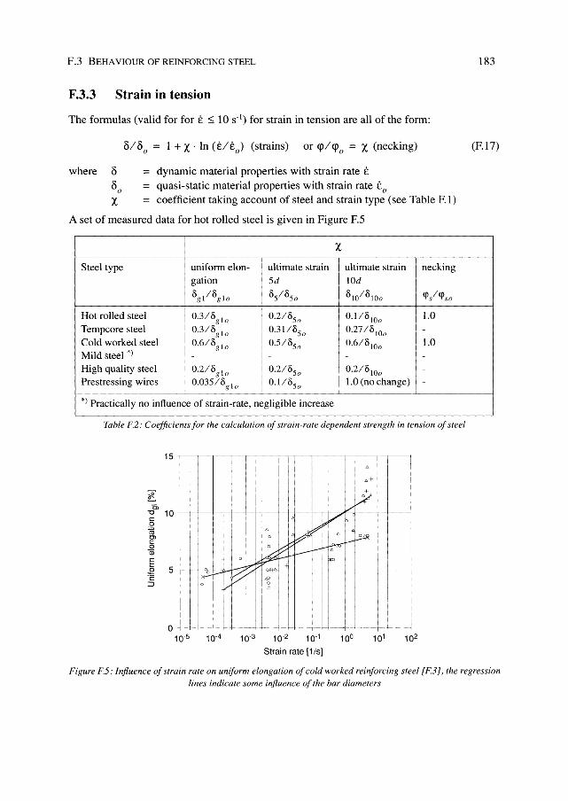
F.3.3 Strain in tension

The fonnulas (valid for for t ~ 10 S·I) for strain in tension are all of the fonn:

0/00 = 1 + X· In (Uta) (strains) or cplcpo = X (necking)

dynamic material properties with strain rate t quasi-static material properties with strain rate to

where 8 80

X coefficient taking account of steel and strain type (see Table F.I)

A set of measured data for hot rolled steel is given in Figure F.5

X

Steel type uniform elon- ultimate strain ultimate strain necking gation 5d lOd

°gl/Ogl0 °51°50 0\0/0\00 q>/q>,w

Hot rolled steel 0.3/0g10 0.2/°50 0.1/°100 1.0 Tempcore steel 0.3/0g10 0.311°50 0.27 18 100

I _

Cold worked steel 0.6/0g10 0.5/°50 0.6/8 100 I

1.0 Mild steel *) - - - -High quality steel 0.2/0g10 0.2/850 0.2/8 100

i I -I

Prestressing wires 0.035/8g10 0.1/850 1.0 (no change) I -I

183

(EI7)

~---,-------

*) Practically no influence of strain-rate, negligible increase

Table F.2: Coefficients for the calculation of strain-rate dependent strength in tension of steel

15 T--'-'---'---~--'--"--'---'-'----'-'--'-----'----I­

~ '" '0 10 "-j--l----I-.'-+--l-c o

1E 0> c o 'iii

E ,g 5-c ~

I I I

I : 0--1- .C-

10,5 10-4 10.3

I I

10'2 10.1

Strain rate [1 Is]

1

1

1

I 102

Figure F5: Influence of strain rate on uniform elongation of cold worked reinforcing steel {F3], the regression lines indicate some influence of the bar diameters

G Dynamic forces from rhythmical human body motions H. Bachmann, A.J. Pret/ave, H. Rainer

G.1 Rhythmical human body motions

Rhythmical human body motions lasting up to 20 seconds and more lead to almost periodic dynamic forces. These can cause more or less steady-state vibrations of structures. Such ac­tivities are often performed to rhythmical music, and if several people are involved, this will practically synchronise their motion. In such cases the dynamic forces increase almost line­arly with the number of participants.

Examples of forcing functions from walking, jumping and hand clapping are given in Figures G.l to G.4. Figure G.4 also gives the relevant continuous Fourier-amplitude spec­trum (see Appendix A). These examples show that not only the frequency of the first harmon­ic of the Fouriertransformation of the forcing function, which is equal to the activity rate (pacing rate, jumping or clapping rate defined as steps per second, jumps per second, claps per second, etc. in Hz) but also the frequencies of upper harmonics may be of importance.

1.5 ,-----~-----,------,_----~-----,----------__, jBoth feet

E .~ 1.0 :;:: u .~

U5

\ \

. ,

\ \ I

I \r~eft foot

o ----"l----o 0.1 0.2 0.3 0.4 0.5 0.6

Time [51

Figure G.] : Forcing function resulting from fooTfall overlap during walking with a pacing rate of 2 Hz [G.4 J

0.7

186 G DYNAMIC FORCES FROM RHYTHMICAL HUMAN BODY MOTIONS

G.2 Representative types of activity

The manifold different types of rhythmical human body motion constitute a large variety of possible dynamic forces. For design purposes, however, the following representative types of activity will be chosen:

- walking - running - jumping - dancing - hand clapping with body bouncing while standing - hand clapping - lateral body swaying

5.0 ~---~---_-______ -,

4.0

Z I

=. 3.0 a.

tp = Contact time

H--+-Tp = Period +-I :

LL CD e 2.0 0

LL

I

-~ -------1 I

1.0

0 0 0.3

Time[s]

Figure G.2: Forcing junction from jumping on the spot with both feet simultaneously at ajumping rate of2 Hz [G.4]

Z 1.5 1.38 kN =. i:r

C!l CD "0

~ 1.0 C. E C1l

~ S 0.5 Q; .§ 0

LL

0 ~

( fp 2 fp 3 fp 4 fp 5 fp

Frequency [ifpJ

Figure G.3: Discrete Fourier amplitude spectrum for the forcing junction from jumping of Figure G.2 up to the fifth harmonic

G.3 NORMALISED DYNAMIC FORCES

a)

b)

o

40 I~-----­I

~ 30 L

J~~~, o 10

2 3 Time [s]

4 5 6 --------- " l I

! , I 20 30 40 50 Frequency [Hz]

187

Figure G.4: Forcing function (a) and continuous Fourier-amplitude spectrum (b) from normal rhythmical hand clapping by a seated person with a clapping rate of 2 Hz [G.5]

Table G.l defines the representative types of activity and gives the relevant ranges of the de­sign activity rates (e.g. pacing, jumping, dancing, hand clapping rate). The columns to the right give the corresponding actual activities and types of structures for which the represent­ative types of activity apply.

G.3 Normalised dynamic forces

To every representative type of activity a normalised dynamic force can be assigned.

The forcing function due to a person's rhythmical body motion can be mathematically de­scribed by a Fourier series of the form ( Appendix A, Equation (A.27) and [G.1], [G.3], [GA]):

where G

n

n

Fp(t) = G+ I.G·a;· sin (21ti//-II» i = 1

weight of the person ("notional pedestrian" of G = 800 N) Fourier coefficient of the i -th harmonic force amplitude of the i -th harmonic equivalent to Ai used in Appendix A activity rate (Hz) phase lag of the i -th harmonic relative to the 1 st harmonic

= number of the i -th harmonic total number of contributing harmonics

(G.l)

188 G DYNAMIC FORCES FROM RHYTHMICAL HUMAN BODY MOTIONS

The graphical representation of the force amplitudes of the harmonics is also called the dis­crete Fourier amplitude spectrum (see Appendix A). An example of the force amplitudes Ga i up to the 5th harmonic of the forcing function of Figure G.2 is given in Figure G.3.

The Fourier coefficients a i and partly also the phase angles <Pi for various human activities have been ascertained in experimental research (e.g. [G.I], [G.21, [G.3], [GA], [G.5]). In Table G.2 pertinent values for the normalised dynamic forces assigned to the representative types of activity of Table G.l are given together with an indication of commonly attained de­sign density of persons.

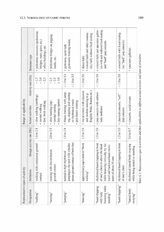
Rep

rese

nlat

ive

type

s of

activ

ity

Ran

ge o

f app

lica

bilit

y

Des

igna

tion

Def

initi

on

Des

ign

activ

ity r

ate

(Hz)

A

ctua

l ac

tiviti

es

Act

ivity

rat

e (H

z]

Stru

ctur

e ty

pe

"wal

king

" w

alki

ng w

ith c

ontin

uous

gro

und

1.6

to 2

,4

• slo

w w

alki

ng (

ambl

ing)

-

1.7

• pe

dest

rian

stru

ctur

es (

pede

stfia

n co

ntac

t •

nonn

al w

alki

ng

-2.

0 br

idge

s, s

lairs

, pi

ers,

ctc

.) •

fast

, br

isk

wal

king

-

2.3

• of

fice

build

ings

. etc

.

"run

ning

" fu

nnin

g w

ith d

isco

ntin

uous

2.

0103

,5

• slo

w r

unni

ng (

jog)

-

2.1

• pe

dest

rian

brid

ges

on jo

ggin

g gr

oun

d co

nlac

l •

nonn

al r

unni

ng

-2.

5 tra

cks,

elc

. •

fast

run

ning

(sp

rint)

> 3.

0

"jum

ping

" no

nnal

LO

high

rhy

thm

ical

1.

8103

.4

• fil

ness

Ira

inin

g w

ith j

ump-

-1.

5 10

3.4

•

gym

nasi

a, sp

an h

alls

ju

mpi

ngon

the

spo

t wilh

sin

lUlta

-in

g, s

kipp

ing

and

funn

ing

• gy

mna

stic

Ira

ini n

g roo

ms

neou

s gr

ound

con

lact

of b

oth

feet

[Q

rhy

thm

ical

mus

ic

-1.

8 to

3.5

•

jazz

dan

ce tr

aini

ng

"dan

cing

" ap

prox

imat

ly e

quiv

alen

t to

"bris

k 1.

5 10

3,0

• so

cial

eve

nts

with

cla

ssic

al

-I.S

to

3.0

• da

nce

halls

w

alki

ng"

and

mod

ern

danc

ing

(e.g

. •

conc

e rt

halls

and

otil

er c

omm

u-E

nglis

h W

altz

. Rum

ba

elc.

) ni

ly h

alls

with

out

fixed

sea

ting

"han

d cl

appi

ng

rhyt

hmic

al h

and

clap

ping

in f

ront

1.

5 to

3.0

•

pop

conc

erts

with

ent

husi

--

I.S to

3.0

• c

once

rt ha

lls a

nd s

pect

ator

gal

ler-

with

bod

y of

one

's ch

esl

or a

bove

the

hea

d as

tic a

udie

nce

ies

with

and

with

out f

ixed

sea

ting

boun

cing

whi

le

whi

le b

ounc

ing

veni

cally

by

for-

and

"har

d" p

op c

once

rts

stan

ding

" w

ard

and

back

war

d kn

ee m

ove-

men

t of

abo

ut 5

0 m

m

"han

d cl

appi

ng"

rhyt

hmic

al h

and

clap

ping

in f

ront

1.5

to 3

.0

• cl

assi

cal c

once

rts,

"so

ft"

-1.

5103

.0

• co

ncer

t ha

lls w

ith f

ixed

sea

ting

of o

ne's

ches

t po

p co

ncer

ts

(no

"har

d" p

op c

Ollc

ens)

"Ial

eral

bod

y rh

ythm

ical

lale

ral

body

sw

ayin

g 0.

4 to

0.7

•

conc

erts

, soc

ial e

vem

s •

spec

tato

r ga

llerie

s sw

ayin

g"

whi

le b

eing

sea

ted

Or

stan

ding

Tabl

e G

,].'

Rep

rese

ntat

ive

type

s of

act

iviti

es a

nd th

eir

appl

icab

ilit

y to

dif

fere

nt a

ctua

l act

iviti

es a

nd ty

pes

of s

truc

ture

s

Cl

\j.l

z o '" ~ f:: Ul

tTl tJ

tJ

--<

Z ~ n (j Q

Vl .....

00

\C

l

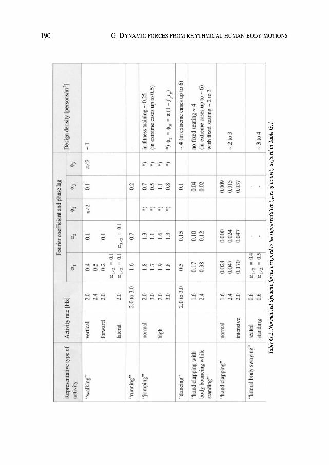
Four

ier c

oeff

icie

nt a

nd p

hase

lag

Rep

rese

ntat

ive

type

of

Act

ivity

rat

e [H

z]

$3

Des

ign

dens

ity [

pers

ons/

m2 ]

aCliv

ity

ct.

ctz

q,z

0:3

"wal

king

" ve

nica

l 2.

0 0.

4 0.

1 ltl

2

01

ltl2

-I

2.4

0.5

forw

ard

2.0

0.2

0.1

(l1

12

= 0

.1

late

ral

2.0

Cl l

/2

= 0

.1

Ct3/

2 '"

0.\

"run

ning

" 2.

0103

.0

1.6

0.7

0.2

-

"jum

ping

" no

rma.l

2.

0 1.

8 1.

3 *)

0.

7 *)

in

fitn

ess

train

ing

-0.

25

3.0

L.7

1.1

*)

0.5

*)

(in e

ICtre

me

case

s up

to 0

.5)

high

2.

0 1.

9 1.

6 *)

1.

1 *)

3.0

1.8

1.3

*)

0.8

*)

*)41

2 =

413

'"

It (

1 -f

/ p)

"dan

cing

" 2.

0103

.0

0.5

0.15

0.

1 -

4 (in

ext

rem

e ca

ses

up to

6)

"han

d cl

appi

ng w

ith

1.6

0.17

0.

10

0.04

no

Ihe

d se

atin

g -

4 bo

dy b

ounc

ing

whi

le

2.4

0.38

0.

12

0.02

(in

ext

rem

e ca

ses

up t

o -6

) st

andi

ng"

with

fixe

d se

atin

g -

2 to

3

"han

d cl

appi

ng"

norm

al

1.6

0.02

4 0.

010

0.00

9 2.

4 0.

047

0.02

4 0.

015

-2 to

3

inte

nsiv

e 2.

0 0.

170

0.04

7 0.

037

"lat

eral

bod

y sw

ayin

g"

seal

ed

0.6

Ctln

=

0.4

-

-st

andi

ng

0.6

Ctln

=

0.5

-

--3

t04

~

Tabl

e G

.2.'

Nor

mal

ized

dyn

amic

forc

es a

ssig

ned

to t

he r

epre

sent

ativ

e ty

pes

of a

ctiv

ity

defin

ed in

Tab

le G

.1

-

- ~ a u -< ~ ~ n 25 S ~ ~ ~ ~ ~ n :.> r ~ ~ Z

I:tI o tl -< ~ ~ '"

H Dynamic effects from wind G. Hirsch, H. Bachmann

H.t Basic theory

H.t.t Wind speed and pressure

Wind is caused by temperature and pressure differences in the atmosphere. The wind blows irregularly over a period of time and its intensity and direction are continually changing. At a particular site and a particular time the wind speed increases over the height of a turbulent boundary layer several hundred meters thick up to the so-called gradient speed, which is no longer influenced by the roughness of the earth's surface. Figure H.l shows a "quasi-station­ary" wind profile, with superimposed stochastically varying turbulences (vortices and wind speed fluctuations):

U tOI (z, t) = U (z) + U (z, t) (H.I)

where u (z) Uz mean wind speed at height z U (z, t) = U z fraction of wind speed due to turbulence utol (z, t) uz, lot gust speed (total speed)

But Ii (z) also changes with time, so that the representation in Figure H.I corresponds to a particular instant in time. Turbulence is caused by flow around different natural and artificial bluff objects and is distributed spectrally over a large range of frequencies.

The wind profile can be described by the following exponential law

where ulO

a

(H.2)

reference wind speed at a height of z ref = 10m above ground in a free field (wind measurements at weather stations) roughness coefficient (a = 0.16 for open country, a = 0.28 for woods, villages and towns, a = 0.40 for large city centres)

The reference wind speed uref = U to (and also uz ) is generally defined for a 10-minute­mean value and a return period of 50 years. Depending on the geographical location of the

192 H DYNAMIC EFFECTS FROM WIND

Gradient wind speed

Wind speed u

Figure H,1.' Wind profile with superimposed turbulence

measuring site, ure! lies usually between 24 and 34 m/s (see e.g, wind map for Europe with lines of equal wind velocity in [H.6]).

u10 and Uz can be related to or converted to other return periods [H.6]. In some codes a ref­erence speed for a 5-second-mean value is used, which corresponds to a factor of 1.4 to 1.5. U 10 can be converted with the help of Equation (H. I ) to the gradient speed (defined at heights of 300 to 500 m depending on the roughness) and vice versa.

The gust fraction u (z, t) and thus the gust speed (total speed) utol are usually defined for the 5-second-mean value of wind measurements.

From the mean wind speed, the wind pressure is

(H.3)

where p = air density (1.2 kg/m3 at normal temperatures)

R.1.2 Statistical characteristics

The stochastic part of the wind speed u (z, t) , which varies over the height above ground and with time, requires the use of statistical methods for the calculation of the dynamic forces on the structure. The basic statistical properties for the variation of the wind speed are described by the following quantities [H.l),[H.6], [H.7). [H.IO]:

- degree of turbulence (turbulence intensity) - power spectral density - correlation between wind speed at several points - probability distribution.

H.l BASIC THEORY

From these the following functions may be derived:

- gust spectrum - aerodynamic admittance function - spectral density of the wind force.

193

These functions are shown in Figure H.2 (symbols which are not defined are not used in this book) and are described qualitatively in the following.

a) Gust spectrum

The time variation of wind speed and thus the wind turbulence at a particular point contains a variety of frequencies with differing amplitudes. A Fourier analysis and some further nu­merical operations allow the turbulence spectrum (= gust spectrum) to be calculated, whose ordinate corresponds to the energy contained in the wind (energy spectrum, spectral density). A peak value in the curve signifies an energy maximum at a particular frequency. Measured spectra usually exhibit a peak at frequencies between 0.05 and 0.01 Hz or between periods of 20 to 100 seconds. Although very large structures (towers, high-rise buildings with fundamen­tal periods in the range 5 to 8 s) and numerous smaller structures (with frequencies of I Hz and beyond) fall into the low energy part of the spectrum, the dynamic response may still be quite significant, especially if the structure's damping is small.

Measured gust spectra exhibit some jagged variation about a mean value, but design spectra are usually presented as smoothed curves (Figure H.2a).

b) Aerodynamic admittance function

There exists a relationship between the gust frequency and its area of influence and therefore between the effect of the gust at a certain frequency and the structure's effective dimensions (e.g. width or square root of width times height/2). Gusts of higher frequency have a smaller area of influence and vice versa, i.e. the lower the frequency of a gust, the larger its area of influence. If small gusts hit a structure of large surface area, only a part of the structure is af­fected and therefore the influence of the gusts is reduced. For a particular surface area this is taken into considcration by the aerodynamic admittance function, which can also be viewed as a surface correction factor (Figure H.2b).

c) Spectral density of the wind force

The product of the gust spectrum and the square of the aerodynamic admittance function gives the spectral density of the wind force, i.e. the force effectively acting on the structure (Figure H.2c).

H.1.3 Dynamic effects

Figure H.3 shows a possible classification of dynamic effects of wind on structures.

Vibrations in the wind direction can result directly from pressure fluctuations of gusts or in­directly from increased turbulence from vortex-shedding in the wake of obstacles (buffeting). The latter etfect belongs to the class of aerodynamic interference between different structures.

194

a) Gust spectrum

f· S(1) 0.3

(Iz u(z))2 0.2

0.1

0.01

b) Aerodynamic admittance function

c) Spectral density of wind

f'S(f) xi (Iz u(z))2

0.01

0.01

Xm 40

30

20

10

d} Mechanical amplification function 1 0.01

~250

(Iz 02 200

150

100

50 I--

e) Spectral density of system response 1 0.01

H DYNAMIC EFFECTS FROM WIND

0.1 10

0.1 10

0.1 10

I d = 0.07 Ie = 0.4

l \..

0.1 10

I I

I

l i I I

I ! I

I 0.1 10

Frequency f [Hz]

Figure H.2: Spectral densities and magnification/unctions

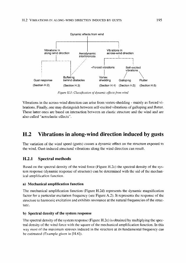
H.2 VIBRATIONS IN ALONG-WIND DIRECTION INDUCED BY GUSTS

Dynamic effects from wind

I

i

Vibrations in along-wind direction Aerodynamic

interferences

Vibrations in across-wind direction

Gust response

(Section H.2)

Buffeting behind obstacles

(Section H.3)

-Forced vibrations

I Vortex shedding

I

Sell-excited vibrations

/ \ Galloping Flutter

(Section H.4) (Section H.5) (Section H.6)

Figure H.3: Classification a/dynamic effects from wind

195

Vibrations in the across-wind direction can arise from vortex-shedding - mainly as forced vi­brations. Finally, one may distinguish between self-excited vibrations of galloping and flutter. These latter ones are based on interaction between an elastic structure and the wind and are also called "aeroelastic effects".

H.2 Vibrations in along-wind direction induced by gusts

The variation of the wind speed (gusts) causes a dynamic effect on the structure exposed to the wind. Gust-induced structural vibrations along the wind direction can result.

H.2.1 Spectral methods

Based on the spectral density of the wind force (Figure H.2c) the spectral density of the sys­tem response (dynamic response of structure) can be determined with the aid of the mechan­ical amplification function.

a) Mechanical amplification function

The mechanical amplification function (Figure H.2d) represents the dynamic magnification factor for a particular excitation frequency (see Figure A.2). It represents the response of the structure to harmonic excitation and exhibits resonance at the natural frequencies of the struc­ture.

b) Spectral density of the system response

The spectral density of the system response (Figure H.2e) is obtained by multiplying the spec­tral density of the wind force with the square of the mechanical amplification function. In this way most of the maximum stresses induced in the structure at its fundamental frequency can be estimated (Example given in [H.6]).

196 H DYNAMIC EFFECTS FROM WIND

H.2.2 Static equivalent force method based on stochastic loading

For structural design purposes the dynamic effect of the wind can be taken into account by defining static equivalent forces.

The static equivalent wind force W can be represented by the following equation [H.5]

where Cfrei

<p cf

A

Ai n Cf i u

W = <p' cf ' Cfrel' A (HA)

(i*1 Cfi' Ai} A

gust factor aerodynamic resistance coefficient of the complete structure according to Figure HA (rectangular cross-sections) and Table H.l (polygonal and cir­cular cross-sections) area of surface loaded by wind area of wind-loaded sub-surface in section i of structure number of sub-surfaces A. of surface A

~ I

p/2· u; = wind pressure on Aj

mean wind speed at height z of sub-surface A j , determined from Equation (H.2) from the reference wind speed u ref = ulO

The gust factor <p considers both the stochastically varying aerodynamic properties of the nat­ural wind and the vibrational behaviour of the structure in its fundamental mode (natural fre­quency and damping). Based on the spectral methods proposed in [H.71 the following equation is also used:

(H.5)

where R terrain factor (roughness factor) according to Figure H.5, which depends on the height of structure h and the statistical peak factor g (i.e. g = 3,5). The straight line in Figure H.5 is valid for ex = 0.16. The value given in Figure H.5 has to be multiplied by l.3 for ex = 0.22 and by l.8 for ex = 0.35 [H.2].

B basic gust factor (takes into account the influence of gusts that are not ampli­fied by the dynamic properties of the structure), and according to Figure H.6, is a function of dl hand h

d = width of structure subjected to wind loading h height of structure s size factor according to Figure H.7 which depends on the "reference frequen-

cy" Ie' hlllh and ratio dlh Ie fundamental frequency of structure in the wind direction 11" mean wind speed at height h F gust energy factor according to Figure H.8, which depends on the wave

number I/u" A damping (expressed as a logarithmic decrement) of the fundamental mode of

the structure (see Chapter 3 and Appendices A, and C)

H.2 VIBRATIONS IN ALONG-WIND DIRECTION INDUCED BY GUSTS 197

The second expression under the square-root sign accounts for the effects of gusts, as en­hanced by the dynamic properties of the structure. Equations (H.4) to (H.6) represent the for­mulas for the spectral analysis method.

1 u polan ;ew h = maximum height of structure

- . ~m dm = mean width perpendicular to wind direction

" 1m = mean length parallel to wind direction

U t "Im~ 3.0

C Q) I '5 2.5

'iJ5 8 Q) 2.0 u c '" u; 1.5

'en ~

. ~ 1.0

'" c ~ 0.5 e Q)

« 0.0

L----t: ----•. :> .... I .-.-.. '

.. ............

--

-

~ ---_ ..........

.' .. ,

.........

--

r- -

f----f.--'

.. ' .. ' .........

.- .-

- -

L , , J I

1 : ! h/dm = i I 50

"1---' I /;20 I ~'r-0- I /1;10

I I / / 5 ' "I.]' ~

, -< 1;2 ,

I r', I '. .?' •

(r'" I l!::~ ~ I -' .... , i~

& i T'T" . .::.:1.:::.::.:

I I I ,

-H+ ,

r- , I

~ ~l -1-- -

0.1 0.2 0.3 0.40.5 2 3 4 5

' , , .I

' iii ' , , , , , , , , , , i , I I ,

, , , , , , i i !

I: i I ,

11 I ,

't- - . 10

Figure H.4: Aerodynamic resistance coefficient for rectangular cross-sections (for cross·sections other than rectangular, use as an approximation the circumscribed rectangle)

I hi dm I Polygon wilh n =

1

Otdmll' I I

-.-i 1 6 1

8 10

2 5

10

20 50

, 0.85 I , 0.90 ,

: 0.80 : 0.85

'1.20 : 1.15 , : 1.35 I 1.25

'1.50 'I 1.40 J

, 0.75 I 0.80 I 1.05

11.20 I 1.30

I Circle with diameter dm = I (Only valid for reinforced concrete structures i because surface roughness coefficient is included) , , , , , , '1m '2m \ I

I 0.65 0.77 0.88 1.00 1.10

I 0.63

: 0.74 I 0.84

0.95 I , , I , 1.05 ,

I : I

3m : 10m : 20m 150m

0.61 I 0.71 , 0.82

I 0.92 I

I 1.02

: 0.60 : 0.70 : 0.80 : 0.90 : 1.00

I 0.54 : 0.63 : 0.72 : 0.81 : 0.90 ,

0.49 0.57

I 1 0 .66 i 0.74 I 0.82

100m

0.48 0.56 0.64

,0.72 0.80

Table H.1: Aerodynamic resistance coefficient for polygonal and circular cross-sections (h = maximum height (?f" structure, d m = mean width perpendicular to wind direction or mean diameter, n = numher of edges)

I 1

I

If it is assumed that the structure vibrates harmonically at its fundamental frequency, then the maximum velocity and acceleration due to the dynamic part of the equivalent wind force W is

where YtO/

(H.6)

bending displacement at the top of the structure due to wind force W from Equation (HA).

198

al (; t5 .E ti5 :;J OJ u

'u; tU III

1.1

1.0 ~i'-, ~ ~ ~

0.8 ~ ~ ~ \\' ~ " .......

0.6 \'\ '-~ '\ ~ "-. '\ "-~ 0.4

" -- ~

0.2 -- --

1 0.0

H DYNAMIC EFFECTS FROM WIND

2.0 - ,- ,-j TIT

1.0 a: 0.8 (; 0.6 ~ 0.5 ~ 0.4 'iii ~ 0.3 I-

0.2

I I 1

I--r---, I

-1 --

f--- - f--f-- - f- -

~ R. = 2g ~ 2.4~ . 0.005 (hi 10) -0. It

HWlth g - 3.5. I I R = 1.2· (hi 10) -0.16 r -=T=t=r:::p:::r:q:Itll+---::r=r~ 0.1

10 20 304050 70 100

Height of structure h [m]

200

Figure H.5: Terrain/actor

900/;' ---,

B-~J-l_. 1 x dx ---' - 9 xh xB (1 + x2) 4/3 o 1 + 400 I + 450

r----.. ,-',-- --,- ,c--- - ---- - J l'---, b. d/h=O ~ ~ r---. ~ 1

~ ~ ~ ~'-k- r--t--- " r-- ---... 1 0.2

"'-.... I'----- I'---- -- 0.:3t::-r--t----r--- ---... -- I

'--

:::-...------- r--- r----.. o. ~::---:L- r--f---r-- ---...1 ___ ---... _1--0.7 r- -

0 r----.. ~ t:--N1.~~ r-- f=::= t-- - - - - :::::: ~ q['1t2 ............ r-- 2.0 r-- - t-- -~ r- :-- -~ I-- 3.0 ~

5.0 f--I Ulil

------1~ --+- --10 20 30 40 50 60 80 100 120 140 160 180 200

Height of structure h [m]

Figure H.6: Basic gust/actor

For the case of gust-induced vibrations of structures in the wind direction it is found that an increase of the structure's damping by an amount normally possible does not result in any sub­stantial decrease of the dynamic response. Passive "mass-dampers" (see Section 3.1.8) offer only slightly better results. This is due to the fact that the peak vibrational response of a struc­ture with various amounts of damping changes little when subjected to a transient (impulse­type) excitation. The dynamic effect of a single gust corresponds more or less to an impulse load. In the past, this fact was generally utilized in the calculation of the wind forces on the structure by deterministic static equivalent force methods.

H.2 VIBRATIONS IN ALONG-WIND DIRECTION INDUCED BY GUSTS

!J)

0 t5 .E! <ll N

Ui

30

2.0

u..

~ 1.0 .E! 0.8 ;.. 0.6 E' <ll 0.5 c 0.4 <ll

Ui 0.3 :::J C}

0.2

1.0

0.7 I --. ..............

0.5 0.4

r-. ........ ' t t:t± - -

0.3 :-.... "No. h. i"-.

0.2 1"-.11- I I

~I K I

0.1 i I 1\ 1\

6.5> [~ ~0.1 l"- I t:d/h=2:0 ~1.0 O} I-- 0

0.07 ,

0.05 I 0.04 I I

0.03 ,

,

0.02

0.01

1 , i,\ \

f I I !' \ \

I I I i [\ l J I! \ \

0.007

0.005 0.004

r --+--"-. r-+t ~~ I " I

t I

0.003

0.002

c-~ ~~L ~ ,-,--,

1 1 R s = ~.

8 f h f ·h I-' l+~·_e_ l+lO·_e_ 1

I 3 uh uh ~ I [, 0.001

0.1 .2 .3.4.5.71.0 2. 3. 4.5. 7.

Reference frequency feh I uh

Figure H.7: Size factor

Wave number fe I uh [11m]

Figure H.8: Gust energy factor

199

j

I~

I

I

,

200 H DYNAMIC EFFECTS FROM WIND

H.2.3 Static equivalent force method based on deterministic loading

The static equivalent force methods based on deterministic loading have been frequently used in the past. However, various assumptions made in the derivation of d are not fully justified from the point of view of the statistical character of wind turbulence. The spectral method and the method derived from it for determining a staLic equivalent foree is thus the preferred one for structural design.

H.2.4 Remedial measures

A rather ineffective measure for reducing the gust-induced vibration in the wind direction - as presented in Appendix H.2.2 - is to increase the damping of the structure. Even mass-dampers are not effective in the case of stochastic single gusts. This is in contrast to buffeting which occurs in urban centres containing numerous high-rise buildings; see Section H.3. The only remaining possibility is in general a st~fler desiRn of the structure.

H.3 Vibrations in along-wind direction induced by buffeting

The airflow behind obstacles exhibits increased turbulence. This can be of a stochastic nature, but it may also consist of regular, i.e. periodic, vortices that are shed in the wake of cylindrical obstacles. These vortices give rise to periodic dynamic forces and act on structures that lie within such an air flow. This phenomenon is called buffeting. Buffeting can lead to substantial vibrations in the wind direction, particularly in the case of resonance, and to correspondingly high stresses in the structure. The frequency of the vortices in the airflow behind the obstacle and thus the frequency of the periodic excitation force acting on the structure is given by

where f w = frequency of vortices S Strouhal number u wind speed [m/s]

fw S·u

d (H.7)

d diameter of obstacle [m] (or the characteristic dimension of body for non-cir-cular section; see Figure H.9 and Table H.2).

The Strouhal number relates the frequency of vortex shedding to a characteristic dimension of the body (e.g. width in across-wind direction) and the speed of air flow. For cylindrical bod­ies it may be assumed that S = 0.2 and is independent of Reynold's number. Figure H.9 shows Strouhal numbers for rectangular sections as a function of the aspect ratio. For other sectional shapes the Strouhal numbers and the corresponding range of Reynold's number are summa­rized in Table H.2.

H.3 VIBRATIONS IN ALO~G-WIND DIRECTION INDUCED BY BUFFETING

0.20

E E 0.15 '" c

Cii -§ 0.10 e if) I

0.05 I o I

o

u D+ ---- d -1

.J1l.

•

-, 2 3 4

Aspect ratio lid

Figure H.9: Stmuhal numbers for rectangular sections

201

The Reynold's number characterizes the ratio of inertia to frictional forces and is defined as

where it -it

d·u Re =--it

kinematic viscosity of the flowing medium -it air = 15· IO--{l m 2/s for practical purposes

(H.8)

At the frequency defined by the Strouhal number, the spectrum of the gusts acting in the wake of a structure is modified. The energy increases at this frequency, but it is difficult to give exact numbers. Often it is necessary to carry out wind tunnel tests to obtain the data.

Of importance is the influence of the ratio of the distance a between the obstacle and the struc­ture (i.e. between the disturbing and the disturbed structures) and the width d of the obstacle. Considerable dynamic effects are obtained over values of aid ranging from about 2 to 16. The maximum is reached at aid of approximately 8 [H.6]. It must also be remembered that the dy­namic effects on existing structures can change significantly when another structure is built in their windward direction. The centres of large cities thus remain in the "construction stage" for as long as other tall buildings are being built.

As a preventive measure against vibrations from buffeting the disturbed structure downwind can be strengthened, thereby increasing its fundamental frequency f e (frequency tuning) and avoiding resonance. However, this is often not possible because the wind speeds can vary be­tween wide limits. Since the wind effect is periodic its influence can be effectively reduced by increasing the damping such as by using mass-dampers. In simple cases the vortex shed­ding behaviour of the disturbing structure can be modified by aerodynamic means (e.g. the Scruton helical stabilizing device, see Sub-Chapter 4.1).

In addition to unfavourable dynamic influences, sheltercd zones can also occur where the sta­tionary wind force is reduced. This effect dies away quickly with int:reasing distance from the disturbing structure. In the case of rectangular-shaped buildings wind shelter effect is negli­gible if the distance-to-width ratio is above 14.

202

a)

b)

H DYNAMIC EFFECTS FROM WIND

Shape of cross-section

I. C<~ ~. 1

- d W r 1 I .:.J w='4

Of ri B 1

I 0=2 - d r 1 I a= '4

r B 1-J Ellipse I 'c=J B - 0=2 I _ t

U1 Ellipse I

I

B 1 I - 0= 2 I , I

Di -(] I , -I

-~~ I I

C---- I

01 I - ,

I

Strouhal number i

S=~ : u_ Valid range

of Reynold's number

I

1

0.33 1 2 x 106 > Re > 4 x 105

0.2 I 5 x 105 > He > 3 x 105

I

0.65 11.6 x 106 > Re > 6 x 105

0.4 I

: 2.5 x 106 > Re > 3 x 105

I I ----I

0.2 -> 0.35 I 6 x 105 > Re > 2 x 105 1 I

0.35

i 1 x 106 > Re > 6 x 105

0.12

i

5 x 105 > He> 3 x 105

0.60 2 x 106 > Re > I x 106

0.2 [

7 x 105 > Re > 1 x 105 I I 1 1 1

022 I I

Re>8x 104 1

0.125 I Re>5x 104

I 0.13 -> 0.22 I Re = 0.3 .. 1.4 x 105

0.14 -> 0.221

I I

1 Re> O.S x 105 I I

~============~~~~~-=~~i~~ - - I . Wind- S f d I Profile Wdl'rie"cdt-"on S = f • A i Profile Wind- S f d I

I I I

;"; __ d_ire_c_tlo_n _=_W_'_U_~---j-, ---,[-",-.~C-d.l--:2-=5d--:---O~7 u~ i -_ '\.. ,"''''''"--'."": I I!d T ~~: , 0.18 I 7 ,d - 0.15 0.5d I d d

lid -, 0.14 ~C f~062d 0.18 I, r f~'L ld 0.12 I 0.18 1 018:.....J

!.2':d I 015 1

I Jd - 0.15 I I!d T 0.16

0.5d

i I~Lld <2: '.-25d 0.5d . -. ~ I ~.., -,.-0.25d

I !d T ~~: i ] [ jd -

~O.~d I' -,.>-_2xO.25d _ 0.15 ~,.

[ Id - 0.14 ] [ ld -0.25! I 0.18

-[-I - 0.17 ,d _ 0.15

0.18

0.15

0.14 0.15

I ___ 0.5d j , ~_-.Jd-

0.14

0.11 0.15

0.16 I

0.20 . ..J

Table H2.· Strouhal numbers a) j(Jr closed sectional shapes, b) for open and for circular sectional shapes [H6 J

HA VIBRATIONS IN ACROSS-WIND DIRECTION INDUCED BY VORTEX-SHEDDING 203

H.4 Vibrations in across-wind direction induced by vortex-shedding

H.4.1 Single structures

For slender cylindrical structures, vortices are shed along the direction of the wind alterna­tively to the left and the right of the cross-section. This produces pulsating excitation forces in the across-wind direction. For vertical structures, such as chimneys etc., the lines of vortex shedding are vertical, i.e. with respect to the height the vortices are always shed at the same place on the cross-section and at the same time. Thus, due to the airflow the structure can be significantly excited especially in the bending mode. If the vortex shedding frequency f w is the same as the natural frequency f e of the structure then resonance occurs. This is the case for the critical wind speed ucr (see Equation (H.7))

(H.9)

Since the process occurs for a structure that is not in motion, one may consider this to be a forced vibration. But it can also lead to a so-called lock-in effect, where due to the motion of the structure the vortex shedding synchronizes with the natural frequency of the structure in a certain range below and above the critical wind speed. As shown in Figure H.1 Oa the vortex shedding frequency remains practically constant in the region of synchronization despite changes in wind speed. The result is a considerable broadening of the region of induced vi­bration. Figure H.lOb shows a narrowband mechanical amplification function which would be decisive for a pure forced vibration for the case of a weakly damped structure (A = 0.01). However, for a critical vortex excitation with lock-in effect, the response amplitudes are in­creased greatly on both sides of the critical wind speed, effectively broadening the amplifica­tion function.

• I

a)

Region of synchronization

Ucr

Wind speed U

~:] b) !VM"h,"~1 •

'O_ID__ • i[1 : /\ amplification

~ I'! \"'" function ~ 0.61 ro i . . ] ! ".~Vortex excitation I 0.4 if\, ! ~ ! \ ~ I / \', A = 0.01

§ Oo2L ... / ~\ (l 0/'-' Ti --T·i·-"'-··-r~Ti ~'Ti--'--"'-' 'i-~--.

o 3 4 5 6 7 8 9 10 11

Reduced wind speed ur

Figure H.IO: Vortex resonance; a) synchronization of vortex shedding and structure frequencies, b) across-wind vibration amplitude (yJd) referred to reduced wind speed ur = u/ dfe

204 H DYNAMIC EFFECTS FROM WIND

The across-wind vibration amplitude y is best related to the dimension d of the cylinder sub­jected to airflow. There are limits to the size of resonance amplification, and these limits are primarily due to the nonlinear aerodynamics at large amplitude vibration. The damping and mass distributions in the stmcture play an important role. Both values are incorporated in the Scmton number, the so-called mass-damping parameter:

where m

Sc = 2· m· A 2

p·d

mass/unit length [kg/m] A logarithmic decrement p air density (1.2 kg/m') d dimension in across-wind direction

(H.IO)

The ratio Yo/ d of the across-wind vibration amplitude Yo at the top of the cantilever to the dimension d may be determined from the following relation given in the draft of DIN 4133, Appendix A (1991):

y/d = 0.123· cL ' (lIS2) . (lISc) (H.ll)

where S Strouhal number (see Equation CH.7» C L aerodynamic lift coefficient S c Scruton number

cL depends on the Reynold's number (see Equation (H.8» and is given in Figure H.11 for a circular cylinder. If two cylinders are located one behind the other, cL increases by a factor 1.5 for a ratio of distance between axes to diameter, aid, less than 15. Such "interference gal­loping" [3.13] can be avoided by use of structural connections. It is interesting to note that wind speed only enters Equation (H.ll) through the Reynold's number (in C L ) and the natural frequency f e does not appear at all, i.e. it cancels out.

An alternative to Equation (H.1l) is obtained by using the amplitude of the dynamic force for the structure under vortex-resonance conditions [DIN 4133]:

P 2 P =c ·_·u ·d

cr L 2 cr (H.12)

The static response to Pcr [N/m] increases with the dynamic amplification factor 1[/ A = 1/ (2S) (case ofresonance due to vortex excitation).

For the case of relatively large damping and widely distributed mass, vortex excitation can also cause critical resonance and can lead to considerable dynamic stresses.

Now a word concerning the conditions at the top of the cantilever and the so-called correlation length. TIle disturbances which emanate from the three-dimensional flow around the end of the cylinder do not form any regular v0l1ices over a distance of about 1.5 diameters from the end. As a result, the correlation length for vortex shedding and thus the dynamic deflection is reduced. In Equation (H.ll) a correlation length was conservatively assumed to be equal to the cylinder length. In general, however, the effective correlation length amounts to about 60% of the cylinder length so that the dynamic deflection would be about 40% less than the value conservatively calculated.

HA VIBRATIONS IN ACROSS-WIND DIRECTION INDUCED BY VORTEX-SHEDDING 205

0.8

cS 0.7 E .~ 0.6

~ o 0.5 <.J

"0 0.4

.~ 0.3 c: >-e 0.2

~ 0.1

o

I I

I I I I

I I I

1 I

I I r-----;---I I I I

104

I I I

I I

I I

I

I

: I I ! I

I i l I ,I

3 5 7 105

1\

1 1\ I

I 1\1 I i\ I

I I I I I

: Ii 3 5 7 106

Reynold number Re

I I

i I

I !

I I

I I

I , -+- 'I

I )(

i I

: II 3 5 7107

Figure H.ll : Aerodynamic lift coefficient for circular cylinder

I I I

3

To calculate the stresses caused by the across-wind vibration amplitude Yo at the top of the cantilever it may be assumed that at maximum deflection the inertia forces are in equilibrium with the elastic defornlation forces in the structure. Therefore the inertia forces can be applied like static forces. With mass m; per increment of length AZi and the normalized mode shape (bending mode), which at height zi of section i has the factor ¢i' the inertia force can be for­mulated at this height as:

F. = m.·¢.·y . (2.n·f·)2 I 1 I 0 e (H.l3)

The normalised mode shape can be extracted from the previous calculation of the bending nat­ural frequency. Alternatively, the following expression can be used:

(n.z.) ¢. = I - cos __ I

, 2·h (H.14)

Figure H.12 shows that for low damping the across-wind vibrations in the case of resonance are approximately harmonic. With increasing damping the vibrations get smaller and tend to become irregular, i.e. they develop a more random character (the representations i), ii), and iii) of Figure H.12a correspond to the zones i), ii), and iii) of Figure H.12b).

If for purposes of approximation it is assumed that the structure vibrates harmonically at its fundamental frequency, then the maximum velocity and acceleration due to the dynamic part of the equivalant wind force W is

where Ytot

(H.l5)

(H.l6)

bending displacement at the top of the structure due to W according to Equation (HA).

206 H DYNAMIC EFFECTS FROM WIND

A preventive measure against vortex-induced vibration in the across-wind direction is to in­crease the critical wind speed, primarily by increasing the fundamental frequency fe (fre­quency tuning). Also effective is an increase of damping possibly using a tuned vibration absorber. In simple cases the Scruton helical device can be used which ensures that the vortex shedding lines are no longer vertical lines but spirals, so that the dynamic effect is considera­bly reduced (cf. Sub-Chapter 3.3).

i} 0

ld l; - 0.5%

a) 'ii) 0

O.ld

0.03d

III) 0

0.03d

• Experimental Re ~ 600000 Height/diameter = 11 .5

:€ 1.2;> 0.10 0.0043 .,

[Ks . 0.54 (1 • ~.2[ onf II> c: 0 Cl. II> "Lock· in" --: e! <» regime ' c (Zone i) ~ ., .c

b) II> max x ., t' 0.01 g t)

'E • III "Transition" c >- regime '0

(Zone ii) E :> E 'x III

~ "Forced vibration" :::i: regime

(Zone iii)

0.001 0.1 0.2 0 .4 0 .60.8 1.0 2 .0 4.0

Figure H.12: Across-wind vibration amplitude of circular cylinder as afunetion of damping (after [H.4])

HA VIBRATIONS IN ACROSS-WIND DIRECTION INDUCED BY VORTEX-SHEDDING 207

H.4.2 Several structures one behind another

The vibrational behaviour described above can change if the vortices emanating from one structure impinge on a second or more structures, e.g. in the case of a row of structures (cf. Appendix H.3), and are superimposed on the other vortex shedding processes. The inter­ference effect that is obtained can lead to an increase of the dynamic reactions, but only if the structures exhibit roughly the same dimensions and dynamic characteristics.

In addition, the Strouhal number is also affected. For circular cylinders the following relation applies:

S = 0.1 + 0.085· log (aid) (H.17)

where a distance from the obstacle (distance between axes) d = diameter

As a result, the Strouhal number reduces from 0.20 (for al d > approx. 15) to 0.14 (for al d approx. 3). Thus the critical wind speed increases by about 40% and the dynamic effect nearly doubles. Consequently, special attention must be paid to the arrangement of similar structures.

H.4.3 Conical structures

Tapered cantilever structures of a conical form can be treated as cylinders if the cone angle is small. The aerodynamic excitation forces, however, already begin to decrease at relatively small cone angles Section H.6.

For cone angles greater than 1.50 two or three frequency ranges exist where separation of the flow occurs. Several Strouhal numbers can be expected. This also occurs if a cylindrical struc­ture changes dimensions stepwise with height. For changes of diameter less than about 5% it is reasonable to assume a constant value (the mean diameter). Otherwise, depending on the actual diameter. different critical wind speeds would be expected.

H.4.4 Vibrations of shells

Finally, under the theme of vortex-induced vibrations, the question of shell vibrations is dis­cussed briefly. There are some well-known cases where such behaviour has led to the collapse of cooling towers. The shell vibrations occur in the form of "ovalizing" with two or three cir­culatory waves observed in the plane. Figure H.I3 shows how the vortex frequencies f w of 1/2 and 1/4 of the natural frequency f e of the shell interact with the two wave forms; the vor­tex shedding force at a certain shell meridian (e.g. left in wind direction) acts always after two and four natural periods of the shell.

The danger of ovalizing vibrations can be effectively minimized by means of stiffening rings. Stiffening measures have to be employed if

where d

dl t ;::.: - 150 (for steel shells)

diameter of the shell thickness of the wall.

(H.I8)

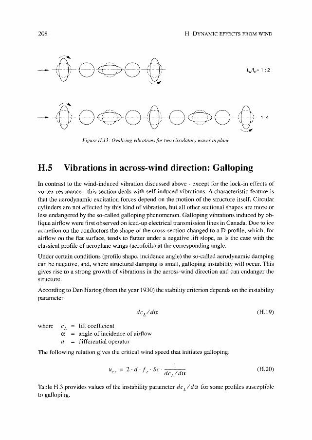
208 H DYNAMIC EFFECTS FROM WIND

V:~~' 8 ..... _-., 8-0-:'''-''-'' - , -, - ~--- ,- . "~ " ". ---_.' ". __ ." ',"_.,.'

~

V:~--~ 8 . ""--', e {:O '''--... 8 ,""---, 8 /(1---'''' - , - . - ~- -. - ,---~~---~, - , " ~ .,.~ " " " ... .' ". __ .'- " ,--- .' ". __ .. ' \. ' .... '

"-=.:tI"

1: 4

Figure H.13: Ovalizing vibrations for two circu/alOry waves in plane

H.S Vibrations in across-wind direction: Galloping

In contrast to the wind-induced vibration discussed above - except for the lock-in effects of vortex resonance - this section deals with self-induced vibrations. A characteristic feature is that the aerodynamic excitation forces depend on the motion of the structure itself. Circular cylinders are not affected by this kind of vibration, but all other sectional shapes are more or less endangered by the so-called galloping phenomenon. Galloping vibrations induced by ob­lique airflow were first observed on iced-up electrical transmission lines in Canada. Due to ice accretion on the conductors the shape of the cross-section changed to a D-profile, which, for airflow on the flat surface, tends to flutter under a negative lift slope, as is the case with the classical profile of aeroplane wings (aerofoils) at the corresponding angle.

Under certain conditions (profile shape, incidence angle) the so-called aerodynamic damping can be negative, and, where structural damping is small, galloping instability will occur. This gives rise to a strong growth of vibrations in the across-wind direction and can endanger the structure.

According to Den Hartog (from the year 1930) the stability criterion depends on the instability parameter

where c L a d

lift coefficient angle of incidence of airflow differential operator

The following relation gives the critical wind speed that initiates galloping:

(H.] 9)

(H.20)

Table H.3 provides values of the instability parameter deLI da for some profiles susceptible to galloping.

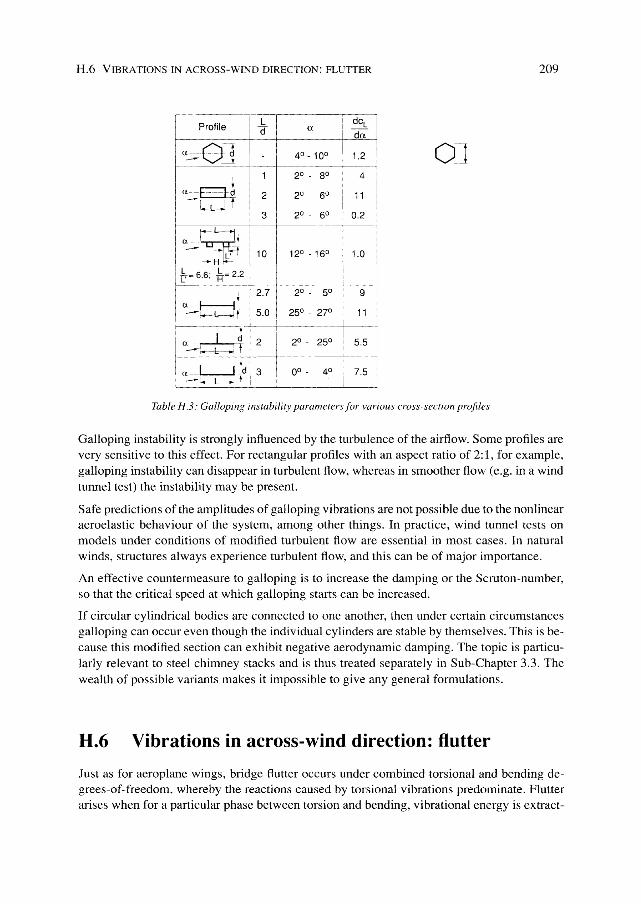
H.6 VIBRATIONS IN ACROSS-WIND DIRECTION: FLUTTER 209

!~------ -LT--~---- -----

I Profile - I a del I d I f--..9.!L I -~

I

a Od -- _1

40 - 100 1.2 OJ 1 2° - 80 4

a-E::::R 2 2° - 60 11 --- ,-,r k-L--..J I

2° - 6° 3 0.2 - - ---------f------- ---- -

'_L~ a-,---~

I - I~~'-: 1 10 120 - 160 1.0

---..rH -

f.= 6.6; -/t= 2.2 I I I

I I

--~ I I 2.7 2° - 5° 9 I

I a-+--L i ---f-.t- - L----.J t 5.0 25° - 27° 11 I

I-.-,

! [--~ J I I 2 2° - 250

~-:~j I O:~I~_b_-': t I I l I a-I [d 13 0° - 4° I i 7.5 I -i--L--': t

~

Table H.3: Gal/oping instability parameters for various cross-section profiles

Galloping instability is strongly influenced by the turbulence of the airflow. Some profiles are very sensitive to this effect. For rectangular profiles with an aspect ratio of 2: l, for example, galloping instability can disappear in turbulent flow, whereas in smoother flow (e.g. in a wind tunnel test) the instability may be present.

Safe predictions of the amplitudes of galloping vibrations are not possible due to the nonlinear aero elastic behaviour of the systcm, among other things. In practice, wind tunnel lcsts on models under conditions of modified turbulent flow arc essential in most cases. In natural winds, structures always experience turbulent flow, and this can be of major importance.

An effective countermeasure to galloping is to increase the damping or the Scruton-number, so that the critical speed at which galloping starts can be increased.

If circular cylindrical bodies are connected to one another, then under certain circumstances galloping can occur even though the individual cylinders are stable by themselves. This is be­cause this modified section can exhibit negative aerodynamic damping. The topic is particu­larly relevant to steel chimney stacks and is thus treated separately in Sub-Chapter 3.3. The wealth of possible variants makes it impossible to give any general formulations.

H.6 Vibrations in across-wind direction: flutter

Just as for aeroplane wings, bridge flutter occurs under combined torsional and bending de­grees-of-freedom, whereby the reactions caused by torsional vibrations predominate. Flutter arises when for a particular phase between torsion and bending, vibrational energy is extract-

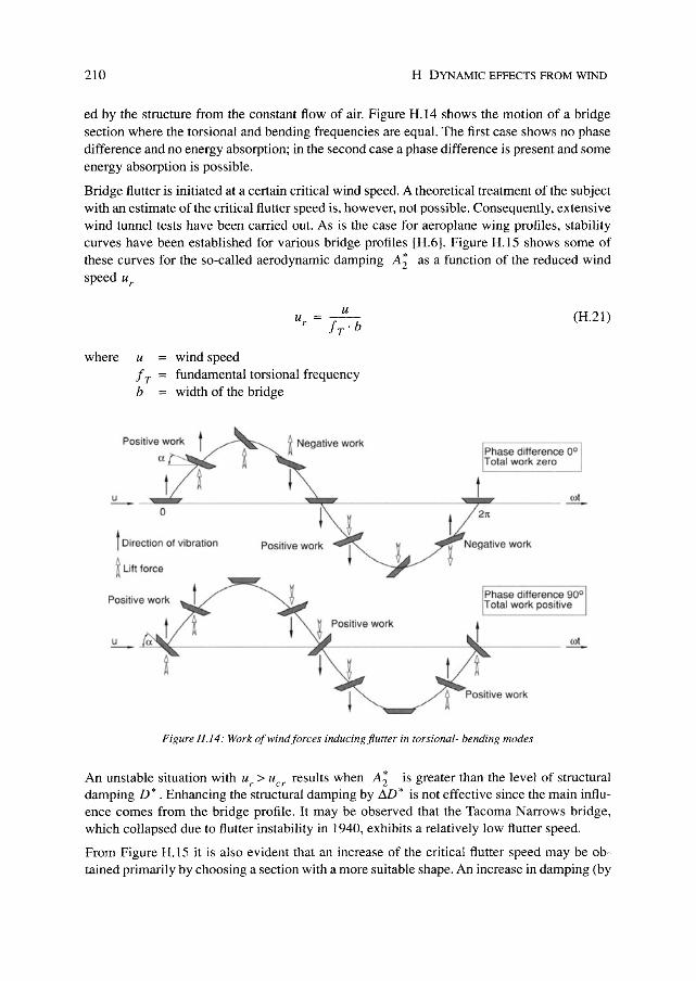
210 H DYNAMIC EFFECTS FROM WIND

ed by the structure from the constant flow of air. Figure H.14 shows the motion of a bridge section where the torsional and bending frequencies are equal. The first case shows no phase difference and no energy absorption; in the second case a phase difference is present and some energy absorption is possible.

Bridge flutter is initiated at a certain critical wind speed. A theoretical treatment of the subject with an estimate of the critical flutter speed is, however, not possible. Consequently, extensive wind tunnel tests have been carried out. As is the case for aeroplane wing profiles, stability curves have been established for various bridge profiles [H.6]. Figure H.lS shows some of these curves for the so-called aerodynamic damping A; as a function of the reduced wind speed ur

where U

iT b

Ur

wind speed fundamental torsional frequency width of the bridge

(H.21)

Phase difference 0° T olal work zero

_U __ ~ __ ~ ________________ ~~~ ________________ ~"L-________ ~ o

I Direction of vibration

~ Lift force

Positive work

Positive work I ~ Negative work

Phase difference 90° T olal work positive

I _u __ ~_"~ ________________ ~~~ ________________ -3~ ________ __ rul

~

Figure H .14: Work o/wind/orees indueingfiutter in torsional- bending modes

An unstable situation with ur > ucr results when A; is greater than the level of structural damping D* . Enhancing the structural damping by W* is not effective since the main influ­ence comes from the bridge profile. It may be observed that the Tacoma Narrows bridge, which collapsed due to flutter instability in 1940, exhibits a relatively low flutter speed.

From Figure H.IS it is also evident that an increase of the critical flutter speed may be ob­tained primarily by choosing a section with a more suitable shape. An increase in damping (by

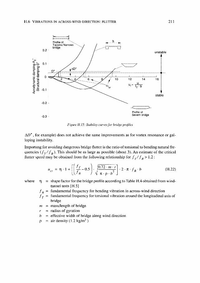
H.6 VIBRATIONS IN ACROSS-WIND DIRECTION: FLUTTER 211

C\l «. 0>0 .~ 0) CoC:: E '0. co E "0 co 0"0

E<a co ~

c::2 >.0 "0 :::J o ~

(j;U) «

0.2 r I 1

I

I I

0.1 r I i I

0 1

-0.1

-0.2 1

1

i -0.3 1

-

t i Profile of ""'" Tacoma Narrows ~~ bridge '

b

12 u

u,= fT'b

14

..L... :::L Profile of Severn bridge

Figure H.15. Stability curves for bridge profiles

unstable

16

stable

j)J)* , for example) does not achieve the same improvements as for vortex resonance or gal­loping instability.

Importang for avoiding dangerous bridge flutter is the ratio of torsional to bending natural fre­quencies (f TI I B)' This should be as large as possible (about 3). An estimate of the critical flutter speed may be obtained from the following relationship for 11'11 B > 1.2:

where 11

IB IT

m

r == h

P

[( IT J ~.72.m.r] Ucr == 11 . I + - - 0.5 . 2.2. 1t . lB' b IB 1t·p·b

(H.22)

shape factor for the bridge profile according to Table H.4 obtained from wind­tunnel tests [H.5] fundamental frequency for bending vibration in across-wind direction fundamental frequency for torsional vibration around the longitudinal axis of bridge mass/length of bridge radius of gyration effective width of bridge along wind direction air density (1.2 kg/m3 )

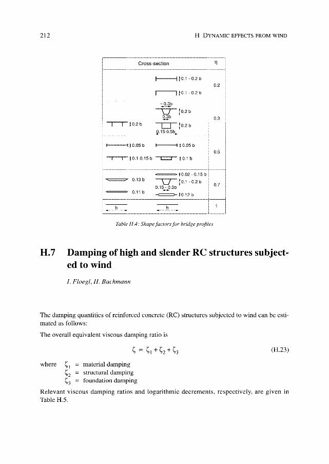
212

H.7

H DYNAMIC EFFECTS FROM WIND

,-----~------------~~,

: Cross-section I 11 !

\.------------ j--~! , I I

i t----11/01 - 0.2 b, ,

: 0.2 ;

1/01-0.2b

{---------i

V j02b

<l1b 0.3

to.2b 0 lO.2b O.15-0.5b ' ____ ~ _____ -.!' ______ J

t----11 10.05 b t----1ljO.05b ,

: 0,5 --r-~ 10.1-0.15 b --rc::::J-"-- 10.1 b :

, ,

----------ti----,

= 0.13b

0.11 b

~==10.02-0.15b I ' ---,,--r- , ,! V jO.l-0.2b , 07 I

0.15 - 0.3b I . I ~ ~ ,

-<==-1012b , I

: ---------j

~~b~ ___ ~_~~b~. ___ ~~ Table 1l.4: Shape factors for bridge profiles

Damping of high and slender RC structures subject­ed to wind

l. Floegl, H. Bachmann

The damping quantities of reinforced concrete (Re) structures subjected to wind can be esti­mated as follows:

The overall equivalent viscous damping ratio is

material damping structural damping foundation damping

(H.23)

Relevant viscous damping ratios and logarithmic decrements, respectively, are given in Table H.S.

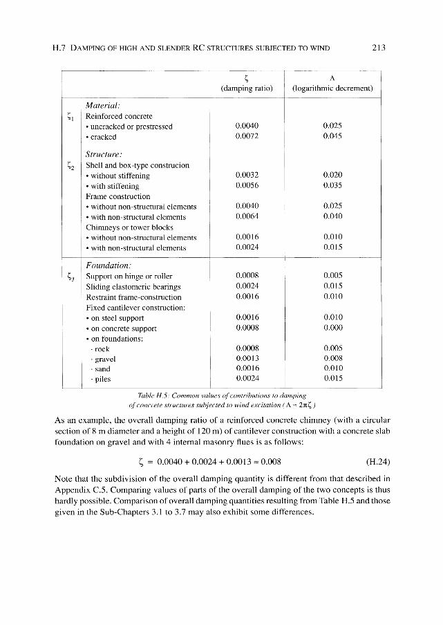
H.7 DAMPING OF HIGH AND SLENDER RC STRUCTURES SUBJECTED TO WIND 213

(damping ratio) (logarithmic decrement)

: Material: ~l I Reinforced concrete

I . un cracked or prestressed : • cracked i ! Structure:

~2 Shell and box-type construcion

I

• without stiffening • with stiffening Frame construction • without non-structural elements • with non-structural elements Chimneys or tower blocks • without non-structural elements • with non-structural elements

i Foundation: ~3 : Support on hinge or roller

: Sliding elastomeric bearings : Restraint frame-construction : Fixed cantilever construction:

II • on steel support I • on concrete support I • on foundations:

· rock · gravel · sand · piles

I I

I

I I

I

I

0.0040 0.0072

0.0032 0.0056

0.0040 0.0064

0.0016 0.0024

0.0008 0.0024 0.0016

0.0016 0.0008

0.0008 0.0013 0.0016 0.0024

I

I

Tahle H.5: Common values of contrihutions to damping of concrete structures sul~jected to ,vind excitation ( /\ ~ 2rr~ )

0.025 0.045

0.020 0.035

0.025 0.040

0.010 0.015

0.005 0.015 0.010

0.010 0.000

0.005 0.008 O.OlD 0.015

~----

As an example, the overall damping ratio of a reinforced concrete chimney (with a circular section of 8 m diameter and a height of 120 m) of cantilever construction with a concrete slab foundation on gravel and with 4 internal masonry flues is as follows:

s = 0.0040 + 0.0024 + 0.0013 "" 0.008 (H.24)

Note that the subdivision of the overall damping quantity is different from that described in Appendix C.S. Comparing values of parts of the overall damping of the two concepts is thus hardly possible. Comparison of overall damping quantities resulting from Table H.5 and those given in the Sub-Chapters 3.1 to 3.7 may also exhibit some differences.

I Human response to vibrations A.J. Pretlave, J.H. Rainer

1.1 Introduction

Human sensitivity to vibration is very acute. The human body can sense vibration displace­ment amplitudes as low as 0.001 mm whilst finger-tips are 20 times more sensitive than this. However, reaction to vibration depends very much on circumstances. For example, discom­fort is different sitting at an office desk from driving a car. Personal attitude is also important. Sensitivity will depend on personal dedication to a task and to acclimatisation. Parameters which affect human sensitivity are as follows:

- position (standing, sitting, lying down) - direction of incidence with respect to the spine - personal activity (resting, walking, running) - sharing of the experience with others - age and sex - frequency of occurrence and time of day - the character of vibration decay.

The intensity of perception will depend upon the following factors:

- displacement, velocity and acceleration amplitudes - duration of exposure - vibration frequency.

The intensity of perception has been researched by many authors and their results are gener­ally in broad agreement with the data in Table 1.1. Broadly speaking, in the range 1 to 10Hz perceptibility is proportional to acceleration, whilst in the range 10 to 100 Hz perceptibility is proportional to velocity. This division varies somewhat with the level of the stimulus but in this basic presentation this factor will be ignored.

1.2 Codes of practice

In order to set realistic criteria, codes of practice also take into account some of the sensitivity factors listed above. Two widely used codes which illustrate the general fcatures described above are [ISO 2631] and [DI~ 4150]. These are discussed in the paragraphs which follow.

216

Description

just perceptible clearly perceptible disturbing/unpleasant intolerable

I HUMAN RESPONSE TO VIBRATIONS

I Frequency range 1 to 10 Hz I Peak acceleration [mm/s2] i

34 100 550

1800

i Frequency range 10 to 100 Hz i Peak velocity [mm/s]

I

I

I

0.5 1.3 6.8

13.8

Table 1.1: An indication of human perceptibility thresholds for vertical harmonic vibrations (person standing). Data combined from various authorities. There is scatter by a factor of up fo about 2 on the values given

1.2.1 ISO 2631

The International Standard lISa 26311 applies to vibrations in both vertical and horizontal di­rections and it deals with random and shock vibration as well as harmonic vibration. The fre­quency range covered is I to 80 Hz and criteria are expressed solely in relation to measured effective accelerations (rms):

(Ll)

T is the period of time over which the effective acceleration is measured.

Note that for pure sinusoidal vibrations the rms value represents 0.707 times the peak value. In [ISO 2631/1] three different levels of human discomfort are distinguished:

- The "reduced comfort boundary", which applies to the threshold at which activities such as eating, reading or writing are disturbed.

- The "fatigue-decreased proficiency boundary", which applies to the level at which recur­rent vibrations cause fatigue to working personnel with consequent reduction in efficiency. This occurs at about three times the reduced comfort boundary.

- The "exposure limit", which defines the maximum tolerable vibration with respect to health and safety and is set at about six times the reduced comfort boundary.

The basic criteria are given in graphical form for both longitudinal vibration (vertical if the subject is standing) and transverse vibration (horizontal if the subject is standing). By way of example, Figure L 1 shows the set of graphical criteria for the longitudinal vibration case. Dif­fcrent criteria apply for different exposure times as indicated on the Figure. This form of pres­entation clearly indicates the adverse effects of body resonances upon acceptability, chiefly resonances within the torso but also those within the cranium. Figure 1.2 shows the corre­sponding set of graphical criteria for transverse vibrations.

For acceptable vibration criteria in buildings [ISO 2631/2] gives base curves to which various suggested multipliers are applied depending on location, duration and time of day.

I.2 CODES OF PRACTICE

~ oS

:a; ",N

c: 0

~ '" a; " " «

20 15 12.5 10

8.0 6.3

5.0

4.0 3.15 2.5

2.0

1.6 1.25

1.0

0.8

0.63 0.50 0.40

0.315 0.25

0.20 0.16 0.125 0.1

L I I ~ --'--

---1 -I I

I 1 1---+ I

I t-- -I

0.32 0.5 0.8 1.25 2.0 3.15 5.0 8.0 12.5 20 31.5 50 80 Hz 0.4 0.63 1.0 1.6 2.5 4.0 6.3 10 16 25 40 63

217

Figure T.l: Bounds on longitudinal vibrationforfatigue-decreased proficiency. The exposure limit is obtained by multiplying by 2; the reduced-comfort boundary by dividing by 3.J5 [ISO 2631/1 j

~ oS '" '" ",0>;

"" "'. ",x

c: 0

~ <l> a; " " «

20

15 12.5 10

8.0 6.3

5.0

4.0 3.15 2.5

2.0 1.6 I·..L

1.25 1.0

0.8 T 0.63 0.50 0.40

0.315 I I I

0.25

0.20

0.16

~ --L--l ------1 ---L---.JJ =~=l==j;;4-;'f'" -----.L_ ~ -------l- ~ I I I I I ;..... I

;------: ~ -ii-~-8Ih I I -I r -: ,- 1-; I : ~ _~ I 1=715~h=' ;==r~--.;7!'--+-+--r--~ _________ ~ ___ -L_,-_I __ -,_~_' _ -_ -L' ==

0.125 .-'-- ~I _I_ . ...L

0.32040.50.630.8101.25162.02.53154.05.06.38.01012516 20 25 31 .540 50 63 80 Hz 0.1

Figure 1.2: Bounds on transverse vibrationforfatigue-decreased proficiency. Factorsfor other boundaries as given in the caption of Figure 1.1 [ISO 263111 )

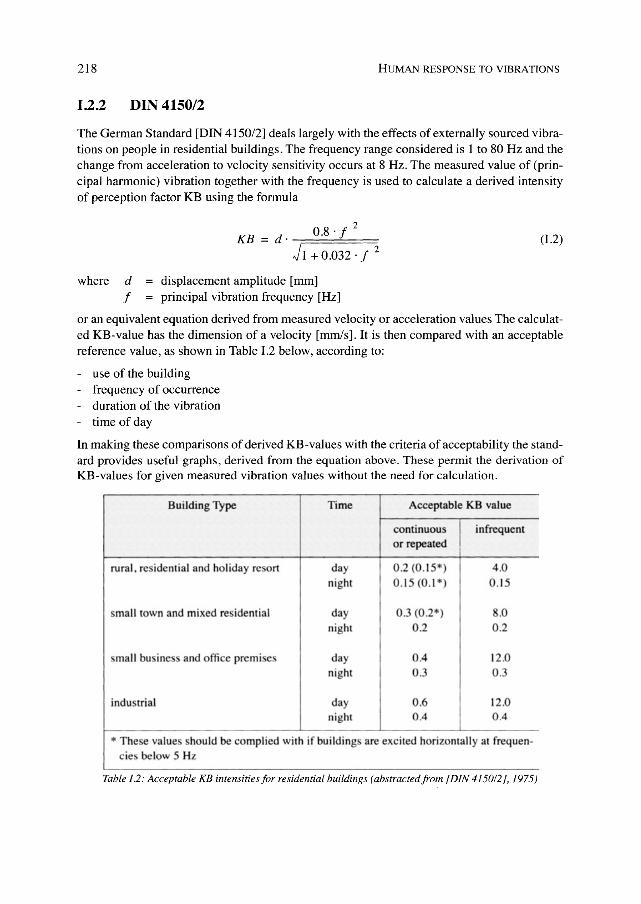
218 HUMAN RESPONSE TO VIBRATIONS

1.2.2 DIN 4150/2

The German Standard [DIN 415012] deals largely with the effects of externally sourced vibra­tions on people in residential buildings. The frequency range considered is 1 to 80 Hz and the change from acceleration to velocity sensitivity occurs at 8 Hz. The measured value of (prin­cipal harmonic) vibration together with the frequency is used to calculate a derived intensity of perception factor KB using the formula

KB 2

= d. 0.8' f Jl+0.032·/ 2

(I.2)

where d displacement amplitude [mm] f = principal vibration frequency [Hz]

or an equivalent equation derived from measured velocity or acceleration values The calculat­ed KB-value has the dimension of a velocity [mm/s].1t is then compared with an acceptable reference value, as shown in Table I.2 below, according to:

- use of the building - frequency of occurrence - duration of the vibration - time of day

In making these comparisons of derived KB-values with the criteria of acceptability the stand­ard provides useful graphs, derived from the equation above. These permit the derivation of KB-values for given measured vibration values without the need for calculation.

Building Type Time Acceptable KB value

continuous infrequent or repeated

rura l. re idential and holiday re ort day 0.2 (0. 15*) 4.0 night 0 .15 (0. 1*) 0.15

small [Own and mixed re idential day 0.3 (0.2*) .0 night 0.2 0 .2

mall bu ine s and office premi e day 0.4 12 .0 night 0.3 0.3

indu [rial day 0.6 12 .0 night 0.4 0.4

* The e value hould be complied wilh if building are exciled horizontally al frequen-cies below 5 Hz

Table 1.2: Acceptable KB intensities/or residential buildings (abstractedJrom [DIN 415012J, 1975)

J Building response to vibrations J.H. Rainer, G. Klein

J.1 General

Serviceability limit states for building structures are those of hairline or minor cracking, spalling of paint or plaster, excessive deflection or accelerated aging.

The recommended values of particle velocity (or sometimes acceleration or displacement) have been obtained by experience and are therefore of an empirical nature. They depend greatly on the type of structure, type of soil and many other parameters whose influence can­not be quantified at present. The values recommended also depend on the type of excitation and the frequency content and duration. For this reason the limit values for blasting differ substantially from those for traffic. It is therefore also not surprising that the tolerable values vary greatly from country to country and from structure to structure, and no single set of cri­teria seems to satisfy all requirements. It should be noted that the recommended criteria do not guarantee absence of damage, but reduce its probability of occurrence to acceptably low levels (see [1.7], [1.2]).

The following are examples of available criteria and standards that are used in some coun­tries; this is, however, not an exhaustive or exclusive list of existing requirements.

The measurement techniques that are associated with these recommendations can vary. Some use the vectorial sum Vi of the instantaneous values

J 2 2 2 v. = V + V + V 1 X Y z (J.1)

others use the maximum value vmax in the direction normal to a wall or in a particular des­ignated direction. Some standards refer to the recommended values at the foundation, others to the ground near the building. The relevant governing quantities will be given with the fol­lowing examples.

220 J BUILDING RESPONSE TO VIBRATIONS

J.2 Examples of recommended limit values

Building Class Frequency range Maximum result-1

Estimated maxi-i where the standard ant velocity, vi

I mum vertical parti-I value is applicable [mm/s] I cle velocity, vma I

[Hz] I [mm/s] I

1. Industrial buildings of rein- 10 - 30 I 12 i 7.2 - 12 'forced concrete, steel con- 30 - 60 12 - l!l 7.2 - 18 struction

2. Buildings on concrete foun- 10 - 30 8 4.8 - 8 dation. Concrete walls or 30 - 60 I 8 - 12 I 4.8 - 12 brick walls I I

1 I

3. Buildings with brick cellar 10 - 30 I 5 I 3-5 I I

walls. Upper apartment 30 - 60 1 5-8 1 3-8 I I

floors on wooden beams I I I I

4. Especally sensitive buildings I 10 - 30 I 3 I 1.8-3 I I

and historical buildings I 30 - 60 I 3-5 I 1.8-5 ! I I

Table l.1: Standard values for piling, sheet piling, vibratory compaction and traffic [J.5]

Maximum vertical particle I I velocity v max [mm/s]

Effect on buildings

--

2 5

I · Risk of damage to ruins and buildings of great historical value • Risk of cracking in normal residential buildings with plastered

walls and ceilings 10 • Risk of damage to normal residential buldings (no plastered

10 - 40 I walls and ceilings)

• Risk of damage to concrete buildings, industrial premises, etc.

Table J.2: Recommended values/or vibratory compactor IJ.3]

Type of building and foundation

• Especially sensitive buildings and buildings of cultural and historical value

• Newly-built buildings and/or foundations of a foot plate (spread footings)

• Buildings on cohesion piles • Buildings on bearing piles or friction piles

Recommended vertical velocity vmax [mm/s]

2

3 5

Table J.3: Recommended limit values for traffic fl.l}

1.2 EXAMPLES OF RECOMMENDED LIMIT VALUES 221

Maximum particle velocity [mm/s] I I

Effects

Sand, Gravel, Clay I Moraine, Slate-stone, I Granite, Gneis, I I I I Lime-stone I Sandstone !

I I I

I I I

18 I

35 I

70 : 0 No noticeable cracking I

30 55 I 110 I 0 Fine cracks and fall of plaster

I I (threshold value) 40 80

I

160 1

0 Cracking 60 115 230 o Serious cracking

Table 1.4: Risk of damage in ordinary dwelling houses with varying ground conditions [f.4J

Type of structure Ground vibration - peak particle velocity, v max [mm/s] (lin/s])

: At low frcquency* < 40 Hz At high frequency> 40 Hz

o Modern homes, drywall interiors o Old homes, plaster on wood, lath

construction for interior walls I

I

I

I

19 (0.75) 13 (0.5)

51 (2.0) 51 (2.0)

1--------- - ------- -----------------------

* All spcctral peaks within 6 dB (50%) amplitude of the predominant rcquency must be analyzed.

Table f.5: Safe levels uf hlasting vibratiuns felT residential type structures [1.6J

Type of structure I Vibration velocity Vj [mm/5] I I At foundation At plane of floor of I

I < 10 Hz 110 - 50 Hz 150 - 100 Hz* uppermost full storey (all frequencies)

I I

I.Buildings used for commer- I 20 I

20 - 40 I 40 - 50 I 40 I

I cial purposes, industrial I I I

I I I i buildings and buildings of I I I

I I I !

similar design I I I I I I

2.Dwcllings and buildings of I 5 I 5 - IS I 15 - 20 15 I I I

similar design andlor use I I I

I I I 3.Structures that, because of I 3 I 3-8 I 8 - 10 8 I I I

their particular sensitivity to I I I

I I

vibration, do not corrcspond I I I I I

I to those listed in lines I and 2

I I

I I !

and are of great intrinsic I I I I I I I I

I value (e.g. buildings that are I

I I I under preservation order) I I I

I I I ---- I --------- - - -

* For frequencies above 100 Hz, at least the values specified in this column shall be applied

Table J.6: Guideline values of vibration velocity for evaluating the effects of short-term vibration lDIN 415013 J

References to the Appendices

[A.I] Thomson W.T: "Theory of Vibration". Third edition. Prentice-Hall International Inc., Englewood Cliffs, New Jersey, 1988.

[A.2) Clough R.W. and Penzien J.: "Dynamics of Structures". McGraw-Hill, New York, 1975.

[C.l) Irvine H.M.: "Structural Dynamics for the Practising Engineer". Allen and Unwin, London, Boston, Sidney, 1986.

[C.2] Dieterle R., Bachmann H.: "Experiments and Models for the Damping Behaviour of Vibrating Rein­forced Concrete Beams in the Uncracked and Cracked Condition". Institut flir Baustatik und Konstruk­tion, ETH Zurich, Bericht Nr. 119, Birkhiiuser Verlag Basel, 1981.

[D.I] Den Hartog J.P.: "Mechanical Vibration~". Fourth edition. McGraw- Hill, New York, 1956.

[D.2) Bachmann H., Ammann W.: "Vibrations in Structures - Induced by Man and Machines". Structural Engineering Documents No. 3e. International Association for Bridge and Structural Engineering (IABSE), Zurich, 1987.

[D.3) Gerasch W.J., Natke H.G.: "Vibration Reduction of Two Structures". International Symposium on Vi­bration Protection in Construction. Scientific report, volume I, pp. 132-142, Leningrad (USSR), 1984.

[DA) Matsumoto Y, Nishioka T., Shiojiri H., Matsuzaki K.: "Dynamic Design of Footbridges". International Association of Bridge and Structural Engineering (IABSE). Proceedings P-17/78, Zurich, 1978.

[D.5) Jones R.T., Pretlove A.J.: "Vibration Absorbers and Bridges". Journal of the Institution of Highway En­gineers, pp. 2-8, 1979.

[D.6) Hunt J.B.: "Dynamic Vibration Absorbers". Mechanical Engineering Publications Ltd., London, 1979.

[D.7) Inman D.J.: "Vibrations, Control, Measurement and Stability". Prentice-Hall International Inc., Engle­wood Cliffs, New Jersey, 1989.

[D.S] Bachmann H., Weber B.: "Tuned Vibration Absorbers for damping of 'lively' structures". Submitted to appear in Structural Engineering International, 1995.

lE.l] Prange B.: "Dynamic Response and Wave Propagation in Soils". Proceedings, Dynamical Methods in Soil and Rock Mechanics, Karlsruhe, 5-16 September, 1977. A.A. Balkema, Rotterdam, 1978.

[E.2] Ewing W.M., Jardetzky W.S., Press F.: "Elastic Waves in Layered Media". McGraw-Hill, New York, 1957.

[E.3] Chouw N., Le R., Schmid G.: "Ausbreitung von Erschutterungen in homogenem Boden; Numerische Untersuchungen mit der Randelementmethode im Frequenzbereich" ("Spreading of Vibrations in Ho­mogeneous Ground; Numerical Investigation by the Boundary Element Method in the Frequency Do­main"). Bauingenieur 65, Heft 9, 1990.

224

rF 11 Comite Euro-International du Beton (CEB): "Concrete Structures Under Impact and Impulsive Loading". Bulletin d'Infonnation No. 187, 1988.

[F.2] Vos E., Reinhardt H.W.: "Influence of Loading Rate on Bond in Reinforced Concrete". Proceedings RILEM-CEB-lABSE-IASS- Intcrassociation Symposium on Concrete Structures under Impact and Im­pUlsive Loading. pp. 170-J 81. Bundes-anstalt flir Materialprlifung (BAM), Berlin, 1982.

[F.3] Ammann W., Mlihlematter M., Bachmann H.: "Versuche an Stahlbeton- und Spannbetontragwerken un­ter stossartiger Beanspruchung, Teil 1: Zugversuche an Bewehrungs- und Spannstahl mit erhiihter Dehn­geschwindigkeit" ("Experiments with Structures of Reinforced and Prestressed Concrete Under Impact Loading, Part 1: Tension Tests on Reinforcing and Prestressing Steel under Elevated Loading Rates"). Institut flir Baustatik und Konstruktion, ETH ZUrich, Versuchsbericht Nr. 7709-1, Birkhauser Verlag Ba­sel, 1982.

[F.4] Berner K.: "Der Einfluss der Dehngeschwindigkeit auf das mechanische Ver-halten von Betonstahlen" ("Influencc of Loading Rate on the Mechanical Behaviour of Reinforcing Steel for Concrete"). 12. For­schungskolloquium des Deutschen Ausschusses flir Stahlbeton, Seiten 181-195, Bundesamt fUr Material­priifung (BAM), Berlin. 19R I.

[G.1] Rainer J.H., Pernica G.: "Vertical Dynamic Forces from Footsteps". Canadian Acoustics, Volume 14, No.2, 12-21, 1986.

[G.2] Tilly G.P', Cullington D.W., Eyre R.: "Dynamic Behaviour of Footbridges". International Association for Bridge and Structural Engineering (lABSE), Surveys S-26/84, Zurich, 1984.

[G.3J Bachmann H., Ammann W.: "Vibrations in Structures - Induced by Man and Machines". Structural Engineering Documents No. 3e, International Association of Bridge and Structural Engineering (IABSE), ZUrich, 1987.

[G.4] Baumann K., Bachmann H.: "Durch Menschen verursachtc dynamischc Lastcn und derenAuswirkungen auf Balkentragwerke" (Man-induced Dynamic Forccs and the Rcsponse of Beam Structures). Institut flir Baustatik und Konstruktion, ETH, Zurich, Versuchsbericht Nr.750 1- 3, Birkhiiuscr Verlag Basel, 1988.

lG.5] Vogt R., Bachmann H.: "Dynamische Lasten durch rhythmisches Klatschen, Fussstampfen und Wippen" (Dynamic Loads from Rhythmic Hand Clapping, Footstamping and Moving Up and Down). Institut fUr Baustatik und Konstruktion, ETH, Zurich, Versuchsbericht Nr. 7501- 4, B irkhiiuser Verlag Basel, 1987.

[H.IJ Kolousek v., Pimer M., Fischer 0., Naprstek J.: "Wind Effects on Civil Engineering Structures". Academia, Praha, 1983.

[H.2] Blevins R.D.: "Flow-Induced Vibration". Van Nostrand Reinhold, New York, 1990.

[H.3] Harris c.: "Shock and Vibration Handbook", 29 Part II: Vibrations of Structures Induced by Wind. Mc­Graw-Hill, New York, 1989.

[H.4] Harris R.T.: "Wind Engineering", 6 ICWE, Australia, 1983, Journal of Wind Engineering and Industrial Aerodynamics, Vol. 13-15, Elsevier, Amsterdam, 1983.

[H.5] Zerna W.: "Gebaudeaerodynamik" ("Aerodynamics of Buildings"). Heft 35/36 Konstruktiver Ingenieur­bau, Ruhr-Universitiit, Bochum, Vulkan-Verlag Dr. W. Classen Nachf., Essen, 1981.

[H.6] Ruscheweyh H.: "Dynamische Windwirkung an Bauwerken" ("Dynamic Actions of Wind on Struc­tures"). Band I und II, Bauverlag, Wiesbaden und Berlin, 1982.

[H.7] Davenport A.G.: "The Application of Statistical Concepts to the Wind Loading of Structures". Proceed­ings of the Institution of Civj I Engineers, 1961.

[H.8] Simiu E., Scanlan R.H.: "Wind Effects on Structures". John Wiley & Sons, New York. 1986.

[H.9] Cook, N.J.: "The Designer's Guide to Wind Loading of Building Structures". Part I, Butterworths, London, 1985.

[H.IO] Sockel H.: "Damping Measures to Control Wind Induced Vibrations". CISM Courses and Lectures No. 335. ISBN 3-211-82516-9. Springer-Verlag Wien, New York, 1994.

225

[J.l] Bonde G., Rundquist G. et al.: "Criteria for Acceptable Traffic- Induced Vibrations". Institute of Techno­logy, Uppsala University, UPTEC R I 42 R. TRAVT-K (in Swedish), 19R I. See also Holmberg et a!., 19R4.

[J.2] Holmberg R., et al.: "Vibrations Generated by Traffic and Building Construction Activities". Swedish Council for Building Research, Stockholm, 1984.

[1.3] Forssblad I.: "Vibratory Soil and Rock Fill Compaction". Dynapac MaskinAB, Solna, Stockholm, 1981.

[JA] Langefors U., Kihlstrom B.: "The Ylodern Technique of Rock Blasting". Third edition, Almqvist &

Wiksel1s Boktryckeri AB, Uppsala, Sweden, 1978.

[I.S] Studer I., Suesstrunk A.: "Swiss Standard for Vibration Damage to Buildings". Proceedings of the Tenth International Conference on Soil Mechanics and Foundation Engineering, Volume 3, pp. 307-312, Stockholm, 1981.

[I.6] Siskind D.E., Stagg M.S., Kopp I.W., Dowding C.H.: "Structure Response and Damage Produced by Ground Vibration from Surface Mine Blasting". U.S. Bureau of Mines, Report of Investigation RI8S07, 1980. U.S. Government Printing Office, Washington DC, 1980.

lJ.7J Dowding C.H.,: "Blast Vibration Monitoring and Control". Page 297. Prentice-Hall International Inc., Englewood Cliffs, New Jersey, 1985.

List of Codes and Standards

[BRE]

[BS 5400]

rBS 6472]

[BS CP 2012/1]

[CSA 84J

[CICINDJ

lDIN 1055/4]

[DIN 4024/1]

[DIN 4024/2]

[DIN 4133]

[DIN 4150/1]

[DIN 4150/2]

rDIN 4150/3]

rDIN 41781

"Vibrations: Building and Human Response". Building Research Establishment (UK), BRE Digest 278,1983.

"Steel, Concrete and Composite Bridges: Specification for Loads". British Standard BS 5400, Part 2, Appendix C, 1978.

"Guide to Evaluation of Human Exposure to Vibration in Bui Idings (1 Hz to 80 Hz)". British Standard BS 6472, 1984.

"Code of Practice for Foundations for Machinery: Foundations for Reciprocating Machines". British Standard Code of Practice BS CP 2012, Part 1,1974.

"'Steel Structures for Buildings". Standard CAN3-S16.I- M84, Appendix G, Cana­dian Standards Association, Rexdale, Ontario, 1984.

"Model Code for Steel Chimneys". Comite International des Cheminees Industriel (CICIND), Beckenham, England.

"Design Loads for Buildings; Imposed Loads; Windloads on Structures Unsuscep­tible to Vibration" (available also in German). Norm DIN 1055 Blatt 4, Deutsches Institut fur Normung, Beuth Verlag GmbH, Berlin, 1986; Aendcrung I 1987.

"Maschinenfundamente; Elastische Sttitzkonstruktionen flir Maschinen mit ro­tierenden Massen" ("Machine Foundations; Elastic Supporting Construction for Machines with Rotating Masses"). Norm DIN 4024 Teil I, Deutsches Institut flir Normung, Beuth Verlag GmbH, Berlin, 1988.

"Maschinenfundamente; Steife (starre) Sttitzkonstruktionen flir Maschinen mit peri­odischer Erregung" ("Machine Foundations; Rigid Supporting Constructions for Machines with Periodic Excitation"). EntwurfNorm DIN 4024 Teil2. Deutsches In­stitut ftir Normung, Beuth Verlag GmbH, Berlin, 1988.

"Schomsteine aus Stahl; Statische-Berechnung und Ausfuhrung" ("Steel Stacks; Structural Analysis and Design"). Norm DIN 4l33, Deutsches Institut flir Norrnung, Beuth Verlag GmbH, Berlin, 1973.

"Erschlitterungen im Bauwesen; Vorermittlung und Messung von Schwingungs­grossen" ("Vibrations in Building; Principles, Predetermination and Measurement of the Amplitude of Oscillations"). Vornorm DIN 4150 Teil 1, Deutsches Institut flir Normung, Beuth Verlag GmbH, Berlin, 1975.

"Erschlitterungen im Bauwesen; Einwirkungen auf Menschen in Gebauden" ("Vibra­tions in Building; Influence on Persons in Buildings"). Vornorm DI:-.i 4150 Teil2 bzw. Entwurf Norm DIN 4150 Teil 2, Deutsches Institut ftir Normung, Beuth Verlag GmbH, Berlin, 1975 bzw. 1990.

"Structural Vibration in Buildings; Effects on Structures" (available also in German). NOim DIN 4150 Teil3, Deutsches 1nslitut flir Normung. Beuth Verlag GmbH, Berlin, 1986.

"Glockentiirme; Berechnung und Ausfiihrung" ("Belltowers: Calculation and Constructional Design"). Norm DIN 4178, Deutsches Institut flir Nonmmg, Beuth Verlag GmbH, Berlin, 1978.

228

[DIN 4563011]

[DIN IEC 651]

[EC 1 :2-4]

[ISO 131]

[ISO 2372]

[ISO 2373]

[ISO 26311 I]

[ISO 263112]

[ISO 3945]

IISO/DIS 4354]

[ISO/DIS 4866]

"Grundlagen der Schallmessung; Physikalische und subjektive Gr6ssen von Schall" ("Bases for Measurement of Sound; Physical and Subjective Measures of Sound"). Norm DIN 45630. Blatt 1, Deutsches Institut fijr Normung, Beuth Verlag GmbH, Berlin, 1971.

"Schallpegelmesser" ("Sound Level Meters"). Norm DIN IEC 651, Deutsches Institut fijr Normung, International Electrotechnical Commission, Beuth Verlag GmbH, Berlin, 1981.

"Basis of design and actions on structures - Wind actions". EUROCODE I, Part 2-4, European Prestandard ENV 1991-2-4, 1994.

"Acoustics - Expression of Physical and Subjective Magnitudes of Sound or Noise in the Air". ISO 131 International Standard Organisation, Geneva 1979.

"Mechanical Vibration of Machines with Operating Speeds from 10 to 200 rev/s -Basis for Specifying Evaluation Standards". ISO 2372, International Standards Oran-isation, Geneva, 1974, Amendement 1,1983.

"Mechanical Vibration of certain Rotating Electrical Machinery with Shaft Heights between 80 and 400 mm - Measurement and Evaluation of the Vibration Severity". ISO 2373, International Standard Organisation, Geneva, 1987.

"Evaluation of Human Exposure to Whole-body Vibration; General Requirements". ISO 2631, Part 1, International Standards Organisation, Geneva, 1985.

"Evaluation of Human Exposure to Whole-body Vibration: Continuous and Shock-in­duced Vibration in Buildings (1 to 80 Hz)". ISO 2631, Part 2, International Standards Organisation, Geneva, 1989.

"Mechanical Vibration of large Rotating Machines with Speed ranging from 10 to 200 r/s - Measurements and Evaluation of Vibration Severity in Situ". ISO 3945, International Standards Organisation. Geneva, 1985.

"Wind actions on structures". Draft ISO/DIS 4354. International Standard Organisa­tion, Geneva, 1991.

"Mechanical Vibration and Shock - Measurement and Evaluation of Vibration Effects on Buildings - Guidelines for the use of Basic Standard Methods". Draft ISO/DIS 4866. International Standard Organisation, Geneva, 1986.

[ISO/DIS 10137] "Bases for Design of Structures - Serviceability of Buildings against Vibration". Draft ISO/DIS 10 137, International Standards Organisation, Geneva, 1991.

[lSO/R 357] "Expression of the Power and Intensity Levels of Sound or Noise", Recommendation ISO/R 357, International Standard Organisation, Geneva, 1963.

[ISO/TC98/SC3IWG2] "Wind Loading (Static and Dynamic)". Draft ISO/TC98/SC3/WG2. International Standard Organisation, Geneva, 1991.

[NBCC 90]

[ONT 83]

[SIA 160]

[S~V 640312]

[VDI 2056]

"Serviceability Criteria for Deflections and Vibrations". Commentary A. Supplement to the National Building Code of Canada. National Research Council Canada, Ottawa, 1990.

Ontario Highway Bridge Design Code. Ontario Ministry of Transportation, Toronto, 1983.

"Actions on Structures". Code SIA 160 (available also in German). Schweizer Inge­nieur- und Architekten-Verein (SIA), Zurich, 1989.

"Erschiitterungen im Bauwesen" ("Vibrations in Construction Work"). SNV 640 312, Schweizerische Normenvereinigung, ZUrich, 1978.

"Beurteilungsmassstabe fiir mechanische Schwingungen von Maschinen" ("Effects of Mechanical Vibrations on Machines"). Richtlinie VDI 2056, Verein Deutscher Inge­nieure, Beuth Verlag GmbH, Berlin, 1964.

I VDI 2057/11

[VDI 2057/2j

[VDI 2057/3]

[VDI 2058/1]

[VDI 2062/1]

[VDI 2062/2]

[VDI 2063]

229

"Einwirkung mechanischer Schwingungen auf den Menschen; Grundlagen; Gliede­rung; Begriffe" ("Effects of Mechanical Vibrations on Peuple: Basics, Structure, Definitions"). Entwurf Richtlinie VDI 2057, Blatt I, Verein Deutscher Ingenieure, Beuth Vcrlag GmbH, Berlin, 1997.

"Einwirkung mechanischer Schwingungen auf den Mcnschen; Bewertung" ("Effects of Mechanical Vibrations on People: Assessment"). Entwurf Richtlinie VDI 2057, Blatt 2, Verein Deutscher Ingenieure, Beuth Verlag GmbH, Berlin, 1987.

"Einwirkung mechanischer Schwingungen auf den Menschen; Beurteilung" ("Effects of Mechanical Vibrations on People: Evaluation"). Entwurf Richtlinie VDI 2057, Blatt 3, Verein Deutscher Ingenieure, Beuth Verlag GmbH, Berlin, 1987.

"Beurteilung von ArbeitsHirm in der Nachbarschaft" ("Evaluation of Industrial Noise in the Environment"). Richtlinie VDI 2058, Blatt I, Verein Deutscher Ingenieure, Beuth Verlag GmbH, Berlin, 1985.

"Schwingungsisolierung: Begriffe und Methuden" ("Vibratiun Isolation: Concepts and Methods"). Richtlinie VDI 2062, Blatt 1, Verein Deutscher Ingenieure, Beuth Verlag GmbH, Berlin, 1976.

"Schwingungsisolierung: Isolierelemente" ("Vibration Isolation: Isolation Ele­ments"). Richtlinie VDI 2062, Blatt 2. Verein Deutscher Ingenieure, Beuth Verlag GmbH, Berlin, 1976.

"Measurement and Evaluation of Mechanical Vibrations of Reciprocating Piston Engines and Piston Compressors" (availahle also in German). Richtlinie VDI 2063, Verein Deutscher Ingenieure, Beuth Verlag GmbH, Berlin. 1985.

Index

The following method is used to indicate: References referring to text page number is shown in regular type References referring to figures page number is shown in italic References referring to tables page number is shown in bold

A Aerodynamic admittance function 193, 194 Ancillary devices 65

B

Bandwidth method 163, J fJ3 Basic gust factor 84, 196 Bell towers 50 Blasting 137, 221 Bridge tlutter 209, 210, 211 Bridges 125 Buffeting 200 Building response to vibrations 219 Buildings (Wind) 74

c Cable-stayed bridges

overall system 102 Pylons 97

Cantilevered roofs 108 Chimneys and Masts 86 Concrete, dynamic behaviour 179 Constant -force excitation 33 Construction Work 129 Construction-induced vibrations 113, 129 Coulomb friction 161,161 Critical damping coefficient 159

D

Damping 157 Bell towers 52, 52 Buildings (wind) 75, 75 Cantilevered roofs 109

Chimneys and masts 90 Definition for SDOF 141, 159 Energy radiation 167, 167 Floors for sport or dance activities 19, 19 Floors with fixed seating and spectator galleries 23 Floors with walking people 12 Ground-transmitted vibrations 67 Guyed masts 94, 96 Heel impact method 14 High diving platforms 25, 26 Hysteresis loop 158 Machine foundations and supports 36, 36 Measurement 162 Non-structural elements 166, 167 Overall values 166 Pedestrian bridges 4, 4 Pylons 99 Reinforced concrete 164, 165 Roads 115 Suspension and cable-stayed bridges 104, 105 Towers (wind) 82, 83 Types 158 Under wind actions 212, 213

Damping factor 157 Dance tloors, see Floors for sport or dance activities Dancing 18, 189, 190 dB, see Decibel scales Decay curve method 162,163 Decibel scales 155

Displacements, velocities and accelerations I S6 Weighting 155

Design rules Bell towers 53 Bridges 128 Buildings (wind) 77 Cantilevered roofs 109 Chimneys and masts 91 Construction-induced vibrations 134, 138 Floors for sport or dance activities 20, 21

232

Floors with fixed seating and spectator galleries 24 Floors with walking people 12, 17 Ground-transmitted vibrations 68, 69 Guyed masts 95 High diving platforms 26 Machine foundations and supports 39, 48 Pedestrian bridges 6, 8 Pylons 100 Railways 120, 121 Roads 116, 117

Structure-borne sound 57, 65 Suspension and cable-stayed bridges 105 Towers (wind) S4

DIN 4150/2218,218 DMF, see Dynamic magnification factor Dynamic actions

Bell towers 50, 51 Bridges 125, 126 Buildings (wind) 75 Cantilevered roofs 109 Chimneys and masts (wind) 86 Construction-induced vibrations 129 Floors for sport or dance activities l8 Floors with fixed seating and spectator galleries 22 Floors with walking people 1 1 Ground-transmitted vibrations 67 Guyed masts 93, 94 High diving platforms 25 Machine foundations and supports 31 Pedestrian bridges 2 Pylons 98 Railways 119 Rhythmical body motion I S5, 189, 190 Roads 114,115 Structure-borne sound 56 Suspension and cable stayed bridges 103 Towers (wind) 81, 81 Wind 191

Dynamic consolidation 137 Dynamic magnification factor 7, 144

Definition for SDOF 143 Dynamic response factor 7

E Equivalent SDOF 150 Excavation 137

F Floating-slab-system 117,117,1/8, 121 Floors for sport or dance activities 18 Floors with fixed seating and spectator galleries 22 Floors with walking people 11 Flutter 103

Footbridges, see Pedestrian bridges Forced vibration 143, 144 Fourier series 145, 147, 148, 187 Fourier Transform 146 Free vibration 141

G Galloping 99, 208, 209 Ground-transmitted vibrations 66, 67

Emission 68 Immission 69 Transmission 69

Gust factor 84, 196 Gust spectrum 193, 194 Gusts 75, 81, 195 Guyed Masts 93

H

Hand clapping 22, 189, 190 Harmonic excitation 143 Heel impact method

Criteria 16 Damping ratio 14 Proced ure 13

High tuning method 12 High-diving platforms 25 Human response to vibrations 215

I-J Impact 34, 34, 46 Impacting parts, actions 31 Impedance 149 Insertion loss 59

Change in cross section 63 Heavy mass 61 Soft spring 62

ISO 2631216,217 Jumping 18, 186, 189, 190

K KB-intensity 218, 218

M

Machine foundations and supports 30 Machinery-induced vibrations 29

Bell towers 50 Groundtransmi tted vibrations 66 Machine foundations and supports 30 Structure-borne sound 56

INDEX

I:--rDEX

Man-induced vibrations 1 Floors for sport or dance activities 18 Floors with fixed seating and "pectator galleries 22 Floors with walking people 11 High-diving platforms 25 Pedestrian bridges 2

Mass-damping-parameter 109 Material behaviour under dynamic actions 177

Concrete 178, 179,180 Reinforcing steel lSI, 182, 1 X2, 1113, 183

N

Natural frequency

o

Bell towers 52 Bridges 127, 127 Buildings (wind) 75, 76 Cantilevel'ed roofs 109 Chimneys and masts 89 Floors 13, 15 Floors for sport or dance activities 19 Floors with fixed seating and spectator galleries 23 Floors with walking people 11 Ground-transmitted vibrations 67 Guyed masts 93 High diving platforms 25 Machine foundations and supports 36 Pedestrian bridges 3, 3 Pylons 99 Roads 115 SDOF 141 Suspension and cable, stayed bridges 103, lO4 Towers (wind) 82

Oscillating parts, actions 31, 33

p

Pedestrian bl'idges 2 Periodic excitation 32, 145 Piling, sheet piling 135 Pylons 97

Q Quadratic excitation 32

R

Railways 119 Rayleigh's method S2 Reinforcing steel, dynamic behaviour 181

Remedial measures Bell towers 54 Bridges 128 Buildings (wind) 7R Cantilevered roofs 110 Chimneys and masts 91 Construction-induced vibrations 139 Floors for sport or dance activities 21

233

Floors with fixed seating and spectator galleries 24 Floors with walking people 17 Ground-transmitted vibrations 70 Guyed masts 96 High diving platforms 27 Machine foundations and supports 49 Pedestrian bridges 9 Pylons 100 Railways 124 Roads 118 Structure-borne sound 65 Suspension and cable-stayed bridges 106 Towers (wind) 85

Reynold's number 201 Rhythmical body motions 185, 189,190 Roads 114 Rotating parts, actions 31, 32 Running 189, 190

s Scruton helical device 91, 206 Scruton number 204 SDOF

Damped vibration 142 DilTercntml cquation 141 Dynamic magnification factor 143 Equivalent to continuous systems 150 Forced vibration 143 Hannonic excitation 143 Impedance 149 Model 160 Natural frequency 141 Periodic excitation 145 Tuning 147 Vibration isolation 149. 149

Single degree of freedom system, see SDOF Sound pressure level 59, 155 Spectator gallcries, sec Floors with fixed seating and

spectator galleries Sport floors, see Floors for sport or dance activities Stiffness criteria

High-diving platforms 26,27 Pedestrian bridges 5

Stochastic excitation 35 Strouhal number 200, 201,202,204 Structure-borne sound 56

Absorption 63

234

Initiation 58 Transmission 58

Suspension and cable-stayed bridges 102 Suspension bridges

overall system 102 Pylons 97

Swaying 22, 189, 190

T Tolerable vibrations

Bell towers 52 Blasting 221 Bridges 127 Buildings (wind) 77, 77 Cantilevered roofs 109 Chimneys and masts 90 Construction induced vibrations 220 Construction-induced vibrations 132, 133 Floors for sport or dance activities 20 Floors with fixed seating and spectator galleries 23 Floors with walking people 12 Ground-transmitted vihrations 6R Guyed masts 95 High diving platforms 26 Machine foundations and supports 37, 38 Pedestrian bridges 6 Pylons 100 Railways 120 Roads J 16 Structure-borne sound 57 Suspension and cable-stayed bridges 105 Towers (wind) 84 Traffic-induced vibrations 220

Towers 80 Traffic-induced vibrations 113

Bridges 125 Railways 119 Roads 114

Transient excitation 34 Tuned vibration absorber 169

Buildings (wind) 78, 79 Differential Equation 169 Floors for sport or dance activities 21 Model 170 Optimum tuning 170, 171 Pedestrian bridges 9, 10 Pylons 98, 100 Towers (wind) 85

Tuning Definition for SDOF 147 High tuning 45 Low tuning 43 Principles 41, 42

Tuning, frequency ranges Bell towers 53

INDEX

Floors for sport or dance activities 20 Floors with fixed seating and spectator galleries 24 High diving platforms 27

v

Machine foundations and supports 42 Pedestrian bridges 6

Vibration isolation 41,43,44, 149, 149 Vibration theory 141 Vibrations induced by machinery 29 Vibrations induced by people I Vibrations induced by traffic and construction

activity 113 Vibrations induced by wind 73 Vibratory compaction 136 Vortex-shedding 81,87,98,108,203

w Walking 2, 11,185,189,190 Wave propagation 173

Attenuation J 75 Wave types 173 Wave velocities 173

Wave velocities 173,174,175 Wind pressure 191 Wind speed 191 Wind-induced vibrations 73

Bridge !lutter 209 Buffeting 200 Buildings 74 Cantilevered roofs 108 Chimneys and masts 86 Galloping 208 Gusts 195 Guyed masts 93 Pylons 97 Suspension and cable-stayed bridges 102 Towers 80 Vortex -shedding 203