a and f stars as probes of outer galactic disc kinematics

MNRAS 475, 1680–1695 (2018) doi:10.1093/mnras/stx3299Advance Access publication 2018 January 5

A and F stars as probes of outer Galactic disc kinematics

A. Harris,1‹ J. E. Drew,1 H. J. Farnhill,1 M. Monguio,1 M. Gebran,2 N. J. Wright,3

J. J. Drake4 and S. E. Sale5

1School of Physics, Astronomy and Mathematics, University of Hertfordshire, College Lane, Hatfield AL10 9AB, UK2Department of Physics and Astronomy, Notre Dame University - Louaize, PO Box 72, Zouk Mikael, Lebanon3Astrophysics Group, Keele University, Keele ST5 5BG, UK4Harvard Smithsonian Center for Astrophysics, Cambridge, MA 02138, USA5Astrophysics Group, School of Physics, University of Exeter, Stocker Road, Exeter EX4 4QL, UK

Accepted 2017 December 19. Received 2017 December 15; in original form 2017 October 27

ABSTRACTPrevious studies of the rotation law in the outer Galactic disc have mainly used gas tracersor clump giants. Here, we explore A and F stars as alternatives: these provide a much densersampling in the outer disc than gas tracers and have experienced significantly less velocityscattering than older clump giants. This first investigation confirms the suitability of A starsin this role. Our work is based on spectroscopy of ∼1300 photometrically selected stars inthe red calcium-triplet region, chosen to mitigate against the effects of interstellar extinction.The stars are located in two low Galactic latitude sightlines, at longitudes � = 118◦, samplingstrong Galactic rotation shear, and � = 178◦, near the anticentre. With the use of MarkovChain Monte Carlo parameter fitting, stellar parameters and radial velocities are measured,and distances computed. The obtained trend of radial velocity with distance is inconsistentwith existing flat or slowly rising rotation laws from gas tracers (Brand & Blitz 1993; Reidet al. 2014). Instead, our results fit in with those obtained by Huang et al. (2016) from discclump giants that favoured rising circular speeds. An alternative interpretation in terms ofspiral arm perturbation is not straight forward. We assess the role that undetected binaries inthe sample and distance error may have in introducing bias, and show that the former is aminor factor. The random errors in our trend of circular velocity are within ±5 km s−1.

Key words: methods: observational – techniques: radial velocities – Galaxy: disc – Galaxy:kinematics and dynamics.

1 IN T RO D U C T I O N

The kinematics of stars outside the Solar Circle is relatively poorlyknown. In addition to setting a constraint on the Galactic potential,secure knowledge of the motions of stars at all radii and longitudesin the Galactic disc facilitates studies of non-axisymmetric motion,such as streaming motions due to spiral density waves or transientwinding arms. Understanding the kinematics of the disc in full,including the rotation law, will help us map out its structure, and setconstraints on its formation and evolution.

Within the disc of the Milky Way, the rotational motion is thedominant component. The IAU recommended standard of the cir-cular velocity at the Sun is 220 km s−1 (Kerr & Lynden-Bell 1986).This result is based mainly on the analysis of tracers of the gaseousinterstellar medium (ISM), including CO, H I 21 cm, and H II ra-dio recombination line observations. In recent decades, the work

� E-mail: [email protected]

of Brand & Blitz (1993) has been particularly influential. How therotation varies outward from the Solar Circle is more challenging tomeasure than within because of the greater reliance on the uncertaindistances to the ISM tracers.

It has been common practice to associate CO and H II radio re-combination lines with star-forming regions whose distances arespecified by spectroscopic parallax. More recent studies have madeuse of masers in star-forming regions with much better defineddistances, and these have begun to favour a higher rotation speed.Honma et al. (2012) used a sample of 52 masers associated withpre-main-sequence stars to find the rotational velocity of the localstandard of rest (LSR) to be between 223 and 248 km s−1, with a flatrotation curve. Reid et al. (2014) took a similar approach, using anexpanded sample of over 100 masers to refine the circular rotationspeed at the Sun to 240 ± 8 km s−1. Bobylev, Bajkova & Shirokova(2016) support a raised circular speed (236 ± 6 km s−1) and a nearlyflat rotation curve, based on a large sample of open clusters.

A feature of the studies to date is a drop in sensitivity with increas-ing Galactocentric radius, RG, as the number or quality of available

C© 2018 The Author(s)Published by Oxford University Press on behalf of the Royal Astronomical Society

Downloaded from https://academic.oup.com/mnras/article-abstract/475/2/1680/4791565by gueston 26 February 2018

mailto:[email protected]

Galactic disc kinematics from A and F stars 1681

measurements declines. In the case of maser measurements, justa handful are available beyond RG ∼ 12 kpc. Similarly, the num-ber of star clusters catalogued at RG ≥ 10 kpc is limited to a fewtens. This is an unavoidable consequence of the inherent low spatialfrequency of these object classes outside the Solar Circle. Hence,Galactic rotation of the outer disc remains highly uncertain.

The frequency of stars at increasingly large Galactocentric radiibecomes much higher than either masers or H II regions and work hasbeen undertaken exploiting helium-burning clump giants that canserve as a form of standard candle (Castellani, Chieffi & Straniero1992). Examples of this, emphasizing measurement of the outerdisc, are the works by Lopez-Corredoira (2014), using proper mo-tions from PPMXL1 and by Huang et al. (2016) using LSS-GAC2

and APOGEE3 radial velocities. As older objects with ages ex-ceeding 1 Gyr, clump giants will be subject to significant kinematicscatter, including asymmetric drift.

In this study, we examine another class of stellar tracer that canalso provide a much denser sampling of the outer disc than is avail-able from ISM tracers. We turn to A/F-type stars. These stars offerthe following advantages: they are intrinsically relatively luminous,with absolute magnitudes in the i band of ∼0 to 3; as youngerobjects (∼100 Myr), they have experienced significantly less scat-tering within the Galactic disc (Dehnen & Binney 1998); and, as weshall show, the A stars especially are efficiently selected from pho-tometric H α surveys. We are able to detect them at useful densitiesout to RG ∼14 kpc. Furthermore, the numbers of A-type stars mostlikely exceed the numbers of clump giants in the outer disc, giventhat the outer disc is younger than the inner disc (Bergemann et al.2014). Our own investigations of photometry from the INT 4 Pho-tometric H α Survey of the Northern Galactic Plane (IPHAS; Drewet al. 2005), used here for target selection, supports this expectation.

We explore radial velocity (RV) measurements of near-main-sequence A/F stars as kinematic tracers in two outer-disc pencilbeams, with a view to future fuller exploitation via spectroscopy onforthcoming massively multiplexed wide-field spectrographs (e.g.WEAVE,5 in construction for the William Herschel Telescope). Togreatly reduce the impact of extinction on the reach of our samples,our observations target the calcium-triplet (CaT) region, in the farred part of the spectrum. Now is a good time to embark on thisinvestigation in view of the imminent release of Gaia astrometry,which will include complementary proper motions of disc stars andsupport improved distance estimates.

We present a method of RV measurement in the CaT part of thespectrum and apply it to a data set of ∼1300 spectra of A- and F-typefield stars, in order to confirm their viability as tracers of Galacticdisc kinematics and to pave the way for more comprehensive use ofthem in future. This first data set is made up of stars in two pencilbeams at Galactic longitudes � = 118◦ and � = 178◦. Our data wereobtained at MMT using the multi-object spectrograph HectoSpec.Section 2 describes the observations obtained and how they were

1 PPMXL (Roeser, Demleitner & Schilbach 2010) is a catalogue of positionsand proper motions referred to the ICRS (International Celestial ReferenceSystem).2 LAMOST Spectroscopic Survey of the Galactic Anticentre (Xiang et al.2017). LAMOST is the Large Sky Area Multi-Object Fibre SpectroscopicTelescope.3 The Apache Point Observatory Galactic Evolution Experiment (DR12release; see Alam et al. 2015).4 Isaac Newton Telescope.5 WHT (William Herschel Telescope) Enhanced Area Velocity Explorer(Dalton et al. 2016).

prepared for analysis. In Section 3, we detail the method used toobtain the RVs and stellar parameters and determine distances. Thederived parameter distributions and error budgets are presented.The results obtained close to the anticentre at � = 178◦, our controldirection, demonstrate the validity of the analysis, while the resultsat � = 118◦ indicate a strong departure from a flat or slowly risingGalactic rotation law (Section 4). In Section 5, we review possiblebias, make comparisons with earlier results, and consider whetherstructure due to spiral arm perturbations may have been detected.Our results turn out to be consistent with the rising section of therotation law presented by Huang et al. (2016) based on disc clumpgiants over the Galactocentric radius range 11–15 kpc. A summaryof our conclusions is given in Section 6.

2 O B S E RVAT I O N S A N D DATA

2.1 Sightline and selection of targets for observation

We chose to study two pencil-beam sightlines located at Galacticco-ordinates � = 178◦, b = 1◦ and � = 118◦, b = 2◦. These werechosen for the following reasons:

(i) In principle, RVs measured at l = 118◦ should sample strongshear in Galactic rotation and hence provide stronger insight intohow the rotation changes with Galactocentric radius outside theSolar Circle. This particular sightline is also one that presents rela-tively low total extinction (Sale et al. 2014) and limited CO emission(Dame, Hartmann & Thaddeus 2001), thereby promising access togreater distances. It is consistent with these properties that there isa raised stellar density visible at this location of up to twice theaverage for the region (see Farnhill et al. 2016). This pencil beammost likely misses the main Perseus spiral arm, since the mainbelt of extinction and CO emission lies at higher latitudes than ourchosen pointing by one to two degrees. It is worth noting that thenecessarily sparse H II region data used by Brand & Blitz (1993)to measure the outer-disc rotation curve revealed little change inapparent RV with distance in this location: all values cluster aroundan LSR value of −50 km s−1. Russeil (2003) reported a departureof −21 ± 10.3 km s−1 from mean circular speed associated with thePerseus Arm.

(ii) Sightlines near the Galactic anticentre intersect the directionof dominant circular motion essentially at right angles, leading tothe expectation of measured RVs close to 0 (in the LSR frame)exhibiting negligible change with increasing distance. We chose toobserve an anticentre sightline so that it serves as a control directlyrevealing e.g. RV measurement bias and the magnitude of kinematicscatter. Again, the particular choice made is of a pencil beam that issubject to relatively light extinction. At l = 178◦, higher extinctionis found a degree away, on and below the Galactic equator.

The targets we observed have magnitudes spanning the range,14.2 ≤ i ≤ 18.5, which are expected to populate a heliocentricdistance range of approximately 2–10 kpc.

The sample was selected using the IPHAS r − i, r − H α colour–colour diagram, as shown in Fig. 1. Drew et al. (2008) describedhow this colour–colour diagram can be used to effectively selectsamples of near-main-sequence early-A stars. The candidate A starswere selected from a strip 0.04 mag wide, just above the early-Areddening line shown in Fig. 1, and the candidate F stars wereselected from a strip 0.08–0.09 mag above the same line. The useof both F and A stars ensure the heliocentric distance distribution iswell sampled, as the selected F stars will lie closer on average thanthe intrinsically brighter A stars.

MNRAS 475, 1680–1695 (2018)Downloaded from https://academic.oup.com/mnras/article-abstract/475/2/1680/4791565by gueston 26 February 2018

1682 A. Harris et al.

Figure 1. IPHAS colour–colour diagram with HectoSpec targets overlaid.The grey points are IPHAS sources with r < 19. The HectoSpec stars fall intwo distinct selection strips: the top strip selecting F-type stars (red points)and the bottom strip selecting A-type stars (blue points). The black line isan empirical unreddened main-sequence track, and the green dashed line isthe early-A reddening line.

2.2 Observations and selection of data for analysis

The spectra were gathered using the MMT’s multi-object spectro-graph, HectoSpec (Fabricant et al. 2005), with the 600 lines mm−1

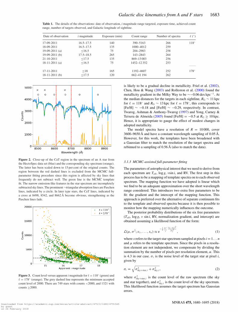
grating providing ∼2.4 Å resolution as measured from narrowsky lines. The observations were performed over six nights in2011 September to November and cover a wavelength range of6532–9045 Å with a sampling of 0.56 Å. Table 1 details the obser-vations on each date, giving the i magnitude range targeted, exposuretime, achieved count range, and number of targets.

The HectoSpec data were reduced using the HSRED6 pipeline,and a mean sky spectrum is determined using dedicated sky fibres.This is subtracted off all target fibres in the same configuration. Anexample of a sky-subtracted spectrum of an A star (blue line) and itscorresponding sky spectrum (orange line) can be seen in Fig. 2. Thewavelength range shown (8470–8940 Å) is the region we use formeasuring RVs and stellar parameters. Whilst much smaller than thetotal range covered by the data, it is chosen as it covers the CaT linesand some prominent Paschen lines. It is also relatively unaffectedby telluric absorption lines. The only other strong photosphericfeature potentially available to us is H α, which is very far awayin wavelength, and close to the blue limit of the MMT spectra.The region between the red dashed lines in Fig. 2 is excludedfrom further analysis since it is particularly dominated by bandsof telluric emission which have proved difficult to subtract cleanlyin many cases. The region also excludes the diffuse interstellar bandat 8620 Å.

A quality cut was applied to the data, accepting spectra with anaverage count level of more than 2000 (between 8475 and 8675 Å),to ensure a large enough signal-to-noise ratio (S/N) for reliableRV and stellar parameter measurements. The wavelength-averagedminimum S/N corresponding to this is 23. There are 887 spectraat � = 118◦ and 434 spectra at � = 178◦ that survive this cut.Fig. 3 shows the count levels versus apparent i magnitude, with thehorizontal line representing the minimum accepted count level. Thedistinct trends are due to weather, varying levels of moonlight, and

6 Information on the latest version of HSRED can be found athttps://www.mmto.org/node/536

exposure time changes (see Table 1). The configurations exposed on19-09-2011 and 18-11-2011, both for targets with i ≤ 16.5, presentcontrasting count levels due to a significant transparency change.The effective magnitude faint limit is i ∼ 17.5–18.

HectoSpec spectra that show signs of red-leak contamination arebetrayed by an upturn in the continuum at the red end reversingthe decline seen shortward of ∼8600 Å. These spectra are removedfrom the sample, leaving 855 target spectra in the � = 118◦ sightlineand 409 in the � = 178◦ sightline.

3 A NA LY SI S O F SPECTRA

3.1 Spectral fitting process

3.1.1 Overview

RVs and the stellar parameters (effective temperature, Teff, surfacegravity, log g, and rotational velocity, vsin i) were measured usingMarkov Chain Monte Carlo (MCMC) full-parameter fits over theCaT range (8470–8940 Å). The target spectra are compared witha template set, interpolated as needed, by mapping the templatesdirectly on to the observations and hence eliminating the need forseparate continuum fitting to both the template spectrum and targetspectrum.

The alternative method of RV measurement by cross-correlationwas also explored. Each target spectrum was cross-correlated withevery template, and the stellar parameters were adopted from thetemplate which produced the tallest cross-correlation function peak.However, a significant weakness of this method is that it does notlend itself easily to error propagation. Consequently, the MCMCmethod has been favoured. The RV measurements for both meth-ods are in agreement within the errors, with a slight bias to morenegative values in the case of cross-correlation. The median dif-ference between MCMC and cross-correlation RV measurementsis 2.0 km s−1 – an amount that falls inside the median RV errorestimate of ∼4.4/6.8 km s−1 for F stars/A stars.

3.1.2 Template spectra

In order to determine the needed quantities from the target spectraobtained, comparisons need to be made with a set of synthetic spec-tra. These synthetic spectra were calculated using the approach ofGebran et al. (2016) and Palacios et al. (2010). These authors haveused SYNSPEC48 (Hubeny & Lanz 1992) to calculate the spec-tra based on ATLAS9 model atmospheres (Kurucz 1992), whichassume local thermodynamic equilibrium, plane parallel geometry,and radiative and hydrostatic equilibrium. We collected 735 spectrathat sample the parameter domain as follows:

(i) [Fe/H] = 0, −0.5(ii) [α/Fe] = 0(iii) 5000 ≤ Teff (K) ≤15000, in steps of 500 K(iv) 3.0 ≤ log g ≤ 5.0, in steps of 0.5(v) 0 ≤ v sin i (km s−1) ≤ 300 km s−1, in steps of 50 km s−1.

The metallicity is not treated as a free parameter: instead we usetwo distinct template sets, one with [Fe/H] = 0 and the other[Fe/H] = −0.5, and compare the results. We do this because ofthe limited spectral coverage and resolution of our data. Our nu-merical trials of metallicity as a free parameter showed it to beunderconstrained and prone to interfere with the descent on to thevalues of other parameters. Nevertheless, there is an expectation thatwith increasing heliocentric distance along both pencil beams, there


https://www.mmto.org/node/536


Table 1. The details of the observations: date of observation, i magnitude range targeted, exposure time, achieved countrange, number of targets observed, and Galactic longitude of sightline.

Date of observation i magnitude Exposure (min) Count range Number of spectra � (◦)

17-09-2011 16.5–17.5 140 390–5163 266 118◦18-09-2011 16.5–17.5 135 1000–4012 25919-09-2011 (a) ≤16.5 75 204–2983 25819-09-2011 (b) 17.5–18.5 265 143–2843 26421-10-2011 ≤17.5 135 869–13 003 25618-11-2011 (a) ≤16.5 75 1452–12 352 253

17-11-2011 ≤18 165 1192–4607 252 178◦18-11-2011 (b) ≤17.5 120 662–41 194 262

Figure 2. Close-up of the CaT region in the spectrum of an A star fromthe HectoSpec data set (blue) and the corresponding sky spectrum (orange).The latter has been scaled down to 15 per cent of the original counts. Theregion between the red dashed lines is excluded from the MCMC full-parameter fitting procedure since this region is affected by sky lines thatfrequently do not subtract well. The green line is the MCMC templatefit. The narrow emission-like features in the star spectrum are incompletelysubtracted sky lines. The prominent ∼triangular absorption lines are Paschenlines, indicated by a circle. In later type stars, the CaT lines, indicated bya cross at 8498, 8542, and 8662 Å become obvious, strengthening as thePaschen lines fade.

Figure 3. Count level versus apparent i magnitude for � = 118◦ (green) and� = 178◦ (orange). The grey dashed line represents the minimum acceptedcount level of 2000. There are 749 stars with counts <2000, and 1321 withcounts ≥2000.

is likely to be a gradual decline in metallicity. Friel et al. (2002),Chen, Hou & Wang (2003) and Rolleston et al. (2000) found themetallicity gradient in the Milky Way to be ∼−0.06 dex kpc−1. Atthe median distances for the targets in each sightline, RG ∼ 11 kpcfor � = 118◦ and RG ∼ 13 kpc for � = 178◦, this corresponds to[Fe/H] ∼ −0.18 and [Fe/H] ∼ −0.29, respectively. In contrast,Twarog, Ashman & Anthony-Twarog (1997) and Yong, Carney &Teixera de Almeida (2005) found [Fe/H] = −0.5 at RG ≥ 10 kpc.Hence, it is appropriate to gauge the effect of modest changes inadopted metallicity.

The model spectra have a resolution of R = 10 000, cover3600–9650 Å and have a constant wavelength sampling of 0.05 Å.However, for this work, the templates have been broadened witha Gaussian filter to match the resolution of the target spectra andrebinned to a sampling of 0.56 Å (also to match the data).

3.1.3 MCMC-assisted full-parameter fitting

The parameters of astrophysical interest that we need to derive fromeach spectrum are Teff, log g, vsin i, and RV. The first step in thisprocess has to be a mapping of template spectra on to each observedspectrum. The mapping function we have adopted is linear whichwe find to be an adequate approximation over the short wavelengthrange considered. This introduces two extra free parameters to befit: the gradient and the intercept of the mapping function. Thisapproach is preferred over the alternative of separate continuum fitsto the template and observed spectra because it is then possible tomonitor how the mapping numerically influences the outcome.

The posterior probability distributions of the six free parameters(Teff, log g, v sin i, RV, normalization gradient, and intercept) areobtained assuming a likelihood function of the form:

L(μ, σ 2; x1, . . . , xn) ∝ e− 1

α

∑i

(xi−μi )2

2σ2i , (1)

where x refers to the target star spectrum sampled at pixels i = 1. . . nand μ refers to the template spectrum. Since the pixels in a resolu-tion element are not independent, we compensate by dividing thesummation by the number of pixels per resolution element, α. Thisis 4.3 in our case. σ i is the noise level of the target star at pixel i,given by

σi =√

σ 2sky+star,i + σ 2

sky,i , (2)

where σ 2sky+star,i is the count level of the raw spectrum (the sky

and star together), and σ 2sky,i is the count level of the sky spectrum.

This likelihood function assumes the target spectrum has Gaussianerrors.



Figure 4. Superposed distributions of measured Teff values (for both sight-lines combined) of stars selected as probably F type (red histogram) andA type (blue histogram). Of the stars initially selected as A type, only12 per cent are cooler F/G stars.

By linearly interpolating the template grid, templates with in-termediate parameter values are produced and hence the modelparameter space is continuous. The RV range is sampled by shift-ing the wavelength axis of the template according to the Dopplerformula.

The ‘EMCEE’ PYTHON package (Foreman-Mackey et al. 2013) isused to execute the MCMC parameter space exploration. Our pro-cedure is set up for 200 ‘walkers’. The priors used are flat for allparameters, with the range available to each parameter matchingthe range in the template set. The range of the RV prior covers allrealistic values (±500 km s−1). The slope and intercept of the func-tion mapping the template on to the target spectrum are nuisanceparameters, for which the range on the prior was determined byexperimentation with the data set. After many steps, the walkersconverge (we use 2000 steps with a 700 step burn-in) and the dis-tribution of parameter values returned by them define the posteriorprobability distribution of the parameters. These are typically ofthe form of a 2D Gaussian. The medians of the marginalized dis-tributions are adopted as the best estimates of parameter values andthe uncertainties are based on the 16th and 84th percentiles. Fig. 2shows an example of a template (green line) with best-estimateparameters for the observed spectrum (blue line).

3.2 Derived stellar parameters

3.2.1 Teff

The measured Teff distribution for both sightlines combined can beseen in Fig. 4. The red bars represent the stars originally selectedfrom the IPHAS r − i, r − H α colour–colour diagram as F stars, andthe blue bars represent the A stars. 78 per cent of the stars selected ascandidate F stars have measured Teff values of 6000–7500 K (typicalof F stars), and 81 per cent of the candidate A stars have Teff valuesof 7500–10 000 K (typical of A stars). It is necessary to point outthat the template set spans temperatures inclusive of G stars (Teff ≤6000 K) and B stars (Teff > 10 000 K). Stars measured as G starsmake up only 2 per cent of the total sample and B stars 4 per cent.These are mainly stars that have contaminated the selected IPHASr − i, r − H α regions. Given the modest levels of contamination(e.g. only 12 per cent of the initial A-star selection turned out to be

cooler than 7500 K), the method of selection is shown to be veryeffective and practically viable. For simplicity in the remainder ofthe paper, we label stars as either F or A type, with Teff = 7500 Kas the boundary dividing them.

The positive and negative errors in Teff as a function of Teff

are shown in the top panel of Fig. 5. The median of the positiveand absolute values of the negative errors combined is ∼150 K;however, the average error increases with temperature and there area number of targets that have large asymmetric errors, betraying anunresolved fit dilemma. As temperature increases, the Paschen linedepths increase until Teff ∼ 9000 K, thereafter they become moreshallow again. This means that there can be a degeneracy where thePaschen line profiles of a lower temperature template are similarto that of a higher temperature template, with the addition of linebroadening effects from the log g and vsin i parameter. This set ofstars, with large Teff errors (>1000 K), consists of only 85 of the1261 targets, and are henceforth removed from the sample. Theseare represented by empty circles in Fig. 5.

Finally, this leaves a total sample made up of 705 A stars(Teff > 7500 K) and 471 F stars (Teff ≤ 7500 K): broken downinto the sightlines, there are 473 A stars and 310 F stars in the� = 118◦ sample, and 232 A stars and 161 F stars in the � = 178◦

sample.

3.2.2 log g

The middle panel of Fig. 5 shows the positive and negative errorsin log g from the posterior distributions as a function of Teff, forthe A and F stars at solar metallicity. It is clear from the figurethat the formal log g error rises steadily with decreasing effectivetemperature. The median error at Teff > 7500 K is 0.09, while belowthis it increases to 0.14. This trend most likely tracks the growingimportance of H− continuum opacity with decreasing effective tem-perature, causing the wings of the CaT lines to become less sensitiveto surface gravity. Gray & Corbally (2009) have noted a ‘dead zone’among mid-late F stars in which dwarf and giant spectra are nearlyindistinguishable.

In F stars with appreciably reduced Paschen line profiles, in par-ticular, this underlying astrophysical trend is compounded to anextent by the moderate spectral resolution of the data. We find forthese cooler stars that the fits begin to exhibit a three-way degen-eracy for combinations of temperature, gravity, and metallicity. Anexample of this degeneracy at work in the CaT in cooler F starswas presented by Smith & Drake (1987). However, with metallicityfixed, it is possible to identify temperature and gravity albeit withgreater error on the latter. The returned F-star log g distribution isskewed strongly in favour of near-MS objects, with a median valueof 4.5 and interquartile range 4.1–4.8, tapering off into a tail reach-ing down to one object with log g � 3.0 (the lower bound on thetemplate set).

The distribution of best-fitting log g values for the A stars can beseen in Fig. 6. The peak of the distribution lies close to where wewould expect it to be. Also shown is the distribution of log g for Astars from a Besancon model (Robin et al. 2003) for � = 118◦, afterconvolving with a Gaussian of σ = 0.09 to emulate the HectoSpecmeasurement error, for a more useful comparison. The measuredHectoSpec distribution has a tail at large values of log g that is notseen in the Besancon model, and its peak is not perfectly matched.A shift of the Besancon distribution of +0.15 brings the two distri-butions into rough alignment. This could be evidence of a bias inour measurements. We appraise the impact of this in Section 5.2.



Figure 5. Positive (red) and negative (blue) errors in Teff (top panel), log g (middle panel) and RV (bottom panel) as a function of Teff. The grey dashed lines inthe top panel represent the Teff error cut: points with |error| >1000 K that are removed from the sample are shown in this figure, represented by empty circles.The green bars connect the positive and negative errors for each individual target.

The stars occupying the high-end tail, which appears more extendedthan in the Besancon model distribution, are mainly cooler objectscarrying larger-than-median errors (see Fig. 5).

3.2.3 vsin i

Fig. 7 shows the measured vsin i distribution for both sightlinescombined, separated into F stars (red bars) and A stars (blue bars).The distribution is as expected, with generally low values for F starsand a spread from low to high values for A stars (Royer 2014). Themedian error on vsin i is ∼20 km s−1, increasing to ∼40 km s−1 forTeff > 10 000 K – as expected for stars that are more commonlyfast rotators. Unsurprisingly, there is evidence of a slight negativecorrelation between individual log g and vsin i parameter fits.

3.2.4 RV

Fig. 5 shows the errors on RV as a function of Teff. The me-dian error is ∼4.4 km s−1 for F stars and ∼6.8 km s−1 for Astars. This difference is attributable to the growing contrast of theCaT lines with decreasing effective temperature. The solar mo-tion needed to convert from the heliocentric to the LSR frame istaken as (U, V, W) = (−11, +12, +7) km s−1 (Schonrich, Binney &Dehnen 2010).

3.3 A comparison with higher resolution long-slit spectra

As a check on the reliability of the derived parameters and theirerrors, we obtained additional long-slit red and blue spectra forseven HectoSpec targets – the positions and apparent i magnitudes



Figure 6. Distribution of measured log g values of A stars for both sightlinescombined (blue histogram). The distribution of log g values of A stars froma Besancon model for � = 118◦ is also shown (green histogram). This hasbeen convolved with a Gaussian of σ = 0.09 to emulate the HectoSpecmeasurement error.

Figure 7. The distributions of measured v sin i values, separated into F stars(red) and A stars (blue), and shown overplotted. The two lines of sight aremerged within each distribution.

Table 2. Positions and apparent i magnitudes of the objects usedfor the HectoSpec-ISIS comparison.

Target RA Dec. i mag ISIS red Teff (K)

1 00:03:41 64:29:43 14.94 7665±115101

2 00:06:36 64:22:38 14.89 7703±7673

3 00:03:47 64:17:12 14.77 7769±8995

4 00:07:37 64:07:51 14.78 8331±2957219

5 00:05:36 63:57:55 14.84 11 043±3441332

6 00:04:02 64:29:49 14.91 11 299±1581710

7 00:07:13 64:46:18 14.82 11 370±202378

of which are shown in Table 2. These were accompanied by five RVstandard stars (with three observed more than once). Of particularinterest in this comparison are the measured surface gravities andRVs. The seven objects reobserved are spread in log g from 3.5to 4.5, as determined from the HectoSpec data, lying across thepeak of the distribution in Fig. 6. The Teff range, again determined

from the HectoSpec data, spans ∼7900–9500 K, with one objectoutside this range with ∼11 900±150

2600 K – the large error indicatingthe unresolved fit dilemma described in Section 3.2.1.

These spectra were gathered as service observations using theIntermediate-dispersion Spectrograph and Imaging System (ISIS)of the 4.2-m William Herschel Telescope during three nights in2016 October to December. ISIS is a high-efficiency, double-armed,medium-resolution (8–121 Å mm−1) spectrograph. The R1200Bgrating was used on the blue arm, and the R1200R grating on thered arm, providing resolution elements for a 1 arcsec slit of 0.85 and0.75 Å, respectively. The wavelength coverage of the blue spectra is3800–4740 Å and of the red spectra is 8110–9120 Å. Both the blueand red spectra have a constant wavelength sampling of 0.22 and0.24 Å, respectively.

The raw images were processed and sky-subtracted and the resul-tant spectra was wavelength calibrated, all with use of the Image Re-duction and Analysis Facility (IRAF). The spectra were then passedthrough the MCMC full-parameter fitting method. For the red spec-tra, the same wavelength limits were adopted as for HectoSpec, andfor the blue the wavelength range used was 4000–4600 Å, cover-ing some of the Balmer series whilst excluding the Ca II K and Hlines since they suffer from interstellar absorption. The measuredparameters and RV were then compared to those measured from theHectoSpec spectra, or to values from the literature in the case of theRV standards, to reveal any systematic differences. A method checkwas performed by comparing the measured parameters from the redand blue ISIS spectra, eliminating the potential for differences dueto a change of instrument. The weighted mean difference betweenmeasured RV for the ISIS RV standard stars and RV from the lit-erature is −0.7 km s−1 for the blue spectra and +0.1 km s−1 for thered spectra. Hence, we are confident that the ISIS wavelength scaleis reliable.

Fig. 8 shows the difference between the ISIS measurements(blue points for blue spectra and red points for red spectra) andthe HectoSpec measurements. The targets are in ascending or-der of Teff, as determined from the ISIS red spectra. In general,the differences in outcome are reassuringly modest and show themethod is working satisfactorily. The dashed lines represent theweighted mean difference between the ISIS red and HectoSpecmeasurements (red line) and ISIS blue and HectoSpec measure-ments (blue line). The weighted mean difference between the redISIS and HectoSpec measurements, and the standard deviation ofthe spread, are: �Teff = −215 ± 1335 K, �log g = −0.36 ± 0.18,�v sin i = −24 ± 53 km s−1 and �RV = −1.9 ± 3.5 km s−1. Thesmall mean difference in measured RV indicates the HectoSpecwavelength calibration is systematically offset by an amount wellbelow measured random errors. The larger difference in log g sug-gests that there may be a bias towards larger values in the HectoSpecdata. This potential bias is not the first evidence: the comparison be-tween our A-star log g distribution and that from a Besancon modelis shown in Section 3.2.2 and we see the HectoSpec distributionpeaks at a slightly larger value. We return to the impact of thispossible bias in Section 5.2.

The blue data points in Fig. 8 provide the comparison betweenthe ISIS blue and HectoSpec data. The weighted mean offsetsand standard deviations obtained are: �Teff = −289 ± 1017 K,�log g = −0.43 ± 0.32, �vsin i = −18 ± 63 km s−1 and �RV= −7.7 ± 8.8 km s−1. As with the red, there is a sizable offset inlog g, suggesting the HectoSpec data may carry a positive bias. TheRV difference is larger than that measured for the red spectra, po-tentially as a result of the fewer absorption lines fitted in the blueregion and hence lower accuracy.



Figure 8. Differences between ISIS and HectoSpec measured stellar parameters. The blue points represent the differences between measurements from theblue ISIS and HectoSpec spectra, and the red points specify differences between the red ISIS and HectoSpec spectra. The targets are in ascending order ofTeff, as determined from the ISIS red spectra. The error shown on each data point is the quadratic sum of the HectoSpec error and ISIS error. The dashed linesrepresent the weighted mean difference between the ISIS red and HectoSpec measurements (red line) and ISIS blue and HectoSpec measurements (blue line).

We have also reviewed the differences between parameters de-rived from the ISIS blue measurements and the ISIS red andHectoSpec data. Hales et al. (2009) performed a similar compar-ison between the red and blue ranges as observed with ISIS, andfound a tendency for the red determined spectral type to be earlierby 0.9 subtypes. They attributed this to strengthening of the Ca II Hand K absorption lines by an interstellar component. Although weexclude these lines in the fitting procedure, we find a modest offsetin effective temperature, with the red suggesting a slightly hotterstar of 112 K with very little change in surface gravity (0.02 dex).

The comparison with higher resolution spectra has provided use-ful insights – the offsets between the ISIS and Hectospec measure-ments are reassuringly modest and are similar to those expecteddue to random errors. Our employed method is working well. Thelarger offset in the derived surface gravities suggest a bias could bepresent to which we will continue to pay attention.

3.4 Extinction, absolute magnitudes, and distance moduli

The distance modulus, μ, of each star is calculated via the followingequation

μ = mi − Ai − Mi, (3)

where mi is the apparent magnitude in the i band, Ai is the extinction,and Mi is the absolute magnitude. The absolute magnitudes usedare from Padova isochrones, interpolated with Teff and log g scales(Bressan et al. 2012; Chen et al. 2015). We choose a value for Mi

on the basis of the median log g and Teff returned by the fits. Wherelog g exceeds the maximum present in the Padova isochrones forthe specified Teff, we reset log g to this value. The median error on

the absolute magnitudes (due to stellar parameter uncertainties) is∼0.3. This is the dominant error source in our final results.

The extinction of each target was calculated using

Ai = 2.5[(r − i)obs − (r − i)int], (4)

where (r − i)obs is the observed colour of the star, taken from IPHASphotometry, and (r − i)int is the intrinsic colour of the star. The in-trinsic colours are calculated from the template grid via syntheticphotometry and the value for each target star is interpolated on thisgrid based on the measured Teff and log g. The coefficient of 2.5 isthe ratio of Ai to Ar −Ai for main-sequence A/F stars with redden-ing levels similar to the HectoSpec data. We use the Fitzpatrick lawwith RV = 3.1. The median error on intrinsic colour (due to stellarparameter uncertainties) is ∼0.01, and on Ai (due to stellar parame-ter and photometric uncertainties) is ∼0.05. After dereddening theobserved magnitudes, μ is obtained: across the entire sample theinterquartile range for the error in μ is 0.2–0.4. The smallest errorsare associated with early A stars (median error ∼0.2).

Fig. 9 shows the Ai extinctions as a function of estimated distancemodulus for both sightlines. Also shown are the mean extinctiontrends due to Sale et al. (2014) across the two pencil beams, includ-ing the expected dispersion in extinction (grey-shaded region). Thiscomparison provides some insight into the plausibility of the dis-tance modulus distribution of our sample. An important differenceto be aware of is that the Sale et al. (2014) trends were computedfrom IPHAS photometry of all probable A-K stars, down to appar-ent magnitudes that are appreciably fainter (to i ∼ 20) than thosetypical of our analysed spectra (i < 18). In both sightlines, thereis evidence that the spectroscopic samples favour lower extinctions



Figure 9. The extinction, Ai, of F stars (red points) and A stars (bluepoints) as a function of distance modulus. Top: � = 118◦, bottom: � = 178◦.Also shown in each panel are the photometrically predicted mean extinctiontrends (grey lines) across the pencil beam (Sale et al. 2014). The grey shadedregion defines the expected dispersion in extinction at every distance withinthe beam. Stars that lie far from the trend in the upper panel are highlightedby a change of colour – orange for the F stars and cyan for one A star. Thiscolouring is preserved in Fig. 11.

than the fainter-weighted photometrically based trends. This is mostlikely a straightforward selection effect.

To check this, we have examined the impact of the counts cutwe placed on the spectra included in the analysis: specifically, wehave compared median estimates of extinction, derived from theirr − i colour, for the stars analysed (counts >2000), with those forlower count stars not analysed. We find that for both directions thecut biases the typical extinction of the A stars (inferred from theavailable r − i colours) to lower values: the strength of effect isthat the unanalysed objects have a median Ai that is greater by 0.4mag. This helps explain the tendency for the blue A-star data points,particularly, to sit lower in Fig. 9. Among the cooler, on-the-whole

closer, F stars there is little difference. The alternative explanationfor this – overlarge distance moduli – runs into difficulty when itis recalled that there may be systematic overestimation of surfacegravities (see Sections 3.2.2 and 3.3). We view this comparison astensioning against accepting and correcting for such a bias in log g,as this would drive up the distance moduli, creating a yet biggeroffset.

3.5 The effect of metallicity

So far all the parameters obtained and described have been com-puted for solar metallicity.

Stellar parameters and RVs have been measured again, asdescribed in Section 3.1.3, but with [Fe/H] set to −0.5 forthe A stars. A new Padova absolute magnitude scale, suitablefor the changed metallicity, was used for determining distancemoduli. The reduced-metallicity fits typically return cooler tem-peratures (�Teff ∼ −400 K). The log g values are also lower(�log g ∼ −0.17), partly compensating for the cooler temperaturesin the estimation of distance. The net effect on the distance modulusscale is a small increase compared with the solar metallicity scale(�μ ∼ +0.12). The RVs measured adopting [Fe/H] = −0.5 areslightly more negative: the median difference is ∼−3.0 km s−1.

In the case of the F stars, there is a growing degeneracy be-tween Teff, log g, and metallicity (see Section 3.2.2). In a trial of[Fe/H] = −0.5 in fitting the F stars, we found the returned gravitiesto be unrealistically low for a population of objects that is morelocalized than the A stars whilst sharing the same faint magnitudelimit. Moreover, it is highly improbable that many among the F-starsample would present [Fe/H] significantly less than 0, since thegreat majority of these fainter objects should lie within a distanceof 5 kpc. We estimate this limiting radius for the case of a warmermain-sequence F star with Teff = 7000 K, i = 17.5 (see Fig. 3),Ai ∼ 1.3 (typical HectoSpec value – see Fig. 9), and Mi = 2.6.At � = 118◦, a distance of 5 kpc corresponds to a Galactocentricradius of ∼10.6 kpc, or a metallicity change of ∼0.2. Consequently,throughout this paper we will fix the metallicity of the HectoSpecF stars at [Fe/H] = 0.

4 T H E S I G H T L I N E R A D I A L V E L O C I T YT R E N D S

The trend of RV with distance modulus can be compared with whatwe would expect to see as an averaged trend if consensus views ofthe Galactic rotation law apply. If all the stars move on circular orbitsabout the Galactic Centre, we would expect to observe a trend of RVsthat are a spread (due to velocity dispersion) around a curve whoseshape depends on the sightline observed, the assumed rotation curve,and LSR parameters (circular velocity and Galactocentric distanceof the LSR, V0, and R0). The comparisons made in this sectionare with a flat rotation curve with LSR parameters R0 = 8.3 kpc,V0 = 240 km s−1, and with the slowly rising rotation curve derivedin Brand & Blitz (1993) with their adopted parameters R0 = 8.5 kpcand V0 = 220 km s−1. We begin with the results for � = 178◦, thecontrol direction, where the rotational component of motion of thestars is effectively nullified.

4.1 � = 178◦

The trend of RV with μ for this pencil beam is shown in Fig. 10. Thered dashed line shows the expected average trend based on a flatrotation curve (although at this sightline the shape of the rotation



Figure 10. The trend of RVs with distance modulus for � = 178◦. The green line is the weighted mean of the RVs of the solar metallicity stars, and the yellowline is obtained on combining [Fe/H] = −0.5 A stars with solar metallicity F stars. The shaded regions represent the standard error of the mean in RV. Theblue points are A stars and the red points F stars, both with metallicity assumed as solar. The red dashed line shows the expected trend for a flat rotation law,which at this sightline will fall close to ∼zero regardless of the V0, R0, or shape of the rotation law adopted.

curve makes little difference). The green line is the weighted meanof the RVs for the solar metallicity stars, plotted as individual datapoints, at each step in μ. The yellow line is the weighted mean forA stars with [Fe/H] = −0.5 and F stars with solar metallicity. Theweighted RV is calculated via the following process:

(i) Every (μ, RV) data point is assigned a normalized Gaussianerror distribution with σ = σμ, where σμ is the error on μ.

(ii) At the ith step (μ = μi), the data points (μn, RVn) witherror distributions in μ overlapping μi are included in forming therunning average, provided |μn − μi | < σμn . The weighting per datapoint is in proportion to the value of its Gaussian error function atμi – thereby taking into account the error in μ in all data points.

(iii) In obtaining the mean RV at μ = μi, the contributing RVvalues are also weighted in proportion to their errors.

(iv) A final weighting is applied in computing the mean in orderthat the contribution from data points at μ < μi balances the contri-bution from data points at μ > μi. This limits the influence of datafrom the most densely populated part of the μ distribution on themean trend.

(v) The minimum number of points required for calculation ofthe mean to either side of μ = μi is 50.

The shaded region around the mean trend line represents its error– the standard error of mean RV at each μi.

In Fig. 10, the F stars dominate the lower end of the range in μ,while the A stars mostly occupy a spread from μ ∼ 12 to μ ∼ 15(or a heliocentric distance range from 2 to 10 kpc). Of the F stars,90 per cent (145 of 165) lie within μ = 11.4–14.5 (d = 1.9–7.8 kpc).90 per cent of the A stars with [Fe/H] = 0 (209 of 232) lie withinμ = 11.8–14.8 (d = 2.3–9.0 kpc), and 90 per cent of the A stars with[Fe/H] = −0.5 (130 of 144) lie within μ = 11.6–15.1 (d = 2.1–10.6 kpc). Ruphy et al. (1996) found a radial cut-off of the stellardisc at RG = 15 ± 2 kpc, and Sale et al. (2010) found that the stellardensity of young stars declines exponentially out to a truncation

radius of RG = 13 ± 0.5statistical ± 0.6systematic kpc, after which thestellar density declines more sharply. The density of our sample inthis sightline also drops off at these distances, but at this stage wecannot be sure whether this decline originates in the Galactic discor is a selection effect.

We find that the overall trend in RV follows the expected flatbehaviour, although it is offset in velocity by a mean amount of3.5 km s−1. The results adopting [Fe/H] = −0.5 for the A stars arevery similar as expected, but with a slightly smaller mean offsetof 3.0 km s−1. There was evidence of a possible small wavelengthcalibration offset arising from the comparison of the HectoSpecobservations with independent higher resolution spectra, effectingthe RV scale by only a couple of km s−1, as described in Section 3.3.Taking these findings together we infer that the RV scale is reliableto within ∼5 km s−1 but cannot rule out the presence of a smallpositive bias in the measurements.

We have computed the RV dispersion of the sample stars, inbroad spectral type groups, around the measured mean trend, in or-der to compare them with the expected dispersions from Dehnen &Binney (1998, see Table 3)). Clearly the measured dispersions arelarger than the Dehnen & Binney (1998) results. Part of this dis-crepancy is attributable to our measurement errors, but the largershare of it may be a consequence of stellar multiplicity. At leasta half of the sample objects are likely to be members of mul-tiple systems, and of those around 15 per cent may be in nearlyequal mass ratio binaries (Duchene & Kraus 2013). Whilst thespectroscopic resolution of our data is insufficient to pick out spec-troscopic binaries, there can nevertheless be binary orbital mo-tions present up to a level of ∼40 km s−1 (depending on phase)in typical cases (for total system masses of 3M, with periodP ∼ 40 d). As the data in Table 3 indicate, the excess dispersionon top of measurement error is in the region of 10 km s−1 forall three spectral type groups. We look at this in more detail inSection 5.



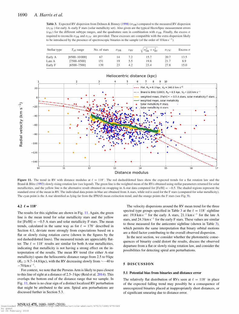
Table 3. Expected RV dispersion from Dehnen & Binney (1998) (σDB) compared to the measured RV dispersion(σ178◦ ) for early A–early F stars (solar metallicity set). Also given are the typical HectoSpec measurement errors(εRV) for the different subtype ranges, and the quadrature sum in combination with σDB. Finally, the excess σ

required to reconcile σDB and σ178◦ are provided. These excesses are compatible with the extra dispersion likelyto be introduced by the presence of spectroscopic binaries in the sample (of the order of 10 km s−1).

Stellar type Teff range No. of stars σDB εRV

√σ 2

DB + ε2RV σ178◦ Excess σ

Early A ]8500–10 000] 67 14 7.2 15.7 20.7 13.5Late A ]7500–8500] 151 19 5.5 19.8 21.7 8.9Early F ]6500–7500] 139 23 4.2 23.4 27.8 15.0

Figure 11. The trend in RV with distance modulus at � = 118◦. The red dashed/dotted lines show the expected trends for a flat rotation law and theBrand & Blitz (1993) slowly rising rotation law (see legend). The green line is the weighted mean of the RVs obtained using stellar parameters returned for solarmetallicities, and the yellow line is the alternative result obtained on swapping in A-star data computed for [Fe/H] = −0.5. The shaded regions represent thestandard error of the mean in RV. The individual data points in blue are obtained from A stars, while red is used for the F stars (computed for solar metallicity).The cyan point is the A star identified as lying far from the IPHAS mean extinction trend, and the orange points the F stars (see Fig. 9).

4.2 � = 118◦

The results for this sightline are shown in Fig. 11. Again, the greenline is the mean trend for solar metallicity stars and the yellowfor [Fe/H] = −0.5 A stars and solar metallicity F stars. The meantrends, calculated in the same way as for � = 178◦ described inSection 4.1, deviate more strongly from expectations based on aflat or slowly rising rotation curve (shown in the figures by thered dashed/dotted lines). The measured trends are appreciably flat-ter. The � = 118◦ results are similar for both A-star metallicities,indicating that metallicity is not having a strong effect on the in-terpretation of the results. The mean RV trend (for either A-starmetallicity) spans the heliocentric distance range from 2.5 to 9 kpc(RG � 9.7–14.8 kpc), with the RV decreasing slowly from ∼−40 to−70 km s−1.

For context, we note that the Perseus Arm is likely to pass closestto this line of sight at a distance of 2.5–3 kpc (Reid et al. 2014). Thisoverlaps the bottom end of the distance range that we sample. InFig. 11, there is no clear sign of a distinct localized RV perturbationthat might be attributed to the arm. Spiral arm perturbations arediscussed further in Section 5.3.

The velocity dispersions around the RV mean trend for the threespectral type groups specified in Table 3 at the � = 118◦ sightlineare: 19.8 km s−1 for the early A stars, 21.1 km s−1 for the late Astars, and 24.3 km s−1 for the early F stars. These values are similarto those measured for the anticentre sightline (shown in Table 3),which permits the same interpretation that binary orbital motionsare a third factor contributing to the overall observed dispersion.

In the next section, we consider whether the photometric conse-quences of binarity could distort the results, discuss the observeddeparture from a flat or slowly rising rotation law, and consider thepossibilities for detecting spiral arm perturbations.

5 D I SCUSSI ON

5.1 Potential bias from binaries and distance error

The relatively flat distribution of RVs seen at � = 118◦ in placeof the expected falling trend may possibly be a consequence ofunrecognized binaries placed at inappropriately short distances, orof significant smearing due to distance error.



Figure 12. The results of simulations to test the effects on the mean RV trend of undetected binaries and distance modulus errors. In the top panel, the purpleline is the mean RV trend for the simulation incorporating unresolved binaries. The orange line is the result from the simulation testing the effect of distancemodulus error only, while the blue line shows the simulated effect of both unresolved binaries and distance modulus errors. The observed RV trend is overlaidin green. In the bottom panel, we test the effect of doubling our distance modulus errors (orange line). The greater error induces more flattening. The lightgreen line in this case is the mean RV trend of the HectoSpec data obtained on adopting doubled distance modulus errors.

If a target star is actually an unresolved binary system, the mea-sured apparent magnitude will be brighter than if it were a singlestar. In effect, the absolute magnitude adopted in our analysis is thentoo low, and hence the distance will be underestimated. Similarly,if the component masses are unequal, the colour will be redder thanif the system were a single star, resulting in overestimation of theextinction and further underestimation of distance. The additionalvelocity component from the motion around another star in a bi-nary system does not produce a bias on the RV results since thespace orientation of binary orbital axes across a large sample israndom and must cancel out. The photometric effect will be mostpronounced in nearly equal mass binary systems, and has beenquantified by Hurley & Tout (1998). Since the binary mass ratiodistribution in A/F stars is not far from flat, we might expect of theorder of 10–20 per cent of our sample to be misconstrued as closerto the Sun by up to 0.75 in μ. In principle, this might erroneouslyflatten the overall RV distribution by bringing in a group of objectsat more negative RV to mix with less negative values at smaller μ.

In order to test the effect of binarity on the calculated weightedaverage RV trend, we have performed an outline simulation thatfocuses on this factor. Our method is as follows. We select threesets of stars of different spectral type groups: early A, late A, andearly F. The size of the sets are the same as the HectoSpec � = 118◦

groups (early A: 168 stars, late A: 281 stars, early F: 259 stars).70 per cent of stars in each group are randomly selected as binaries– these are assigned a primary mass, m1, and the secondary mass,m2, is assigned at random according to a mass ratio fraction, q,obeying the distribution f(q) = q−0.5 (Duchene & Kraus 2013). Thedistance modulus assigned to each star is sampled from the Hec-toSpec μ distribution for its spectral type group. In order to com-pensate for the expected net decrease in μ associated with treatingoutput binary stars as single, these reference distributions are first

modified by a uniform retrospectively determined shift of +0.16.The assigned RVs follow a flat rotation curve with V0 = 240 km s−1

at � = 118◦, broadened by an amount consistent with the scatterdefined by Dehnen & Binney (1998) and measurement error. Thefinal adjustment is to include a component of binary orbital motion.To achieve this, a period, P, inclination, i, and phase, φ, must berandomly assigned for each binary star. The period is selected fromthe distribution of A-star periods shown in fig. 2 in Duchene &Kraus (2013). The inclination is chosen from a uniform distributionin cos i, and the phase from a uniform distribution between 0 and2π . In the final reconstruction of the observed RV distribution, eachsimulated binary star has its distance modulus reduced to the equiv-alent single value according to the computed difference in intrinsiccolour and absolute magnitude.

The simulation of 708 stars was performed 10 000 times, and themean RV trend was calculated each time. The mean of these 10 000trends is shown as the purple line in Fig. 12. The binary stars arepulled by varying amounts to shorter distances and bring with themtheir on-average more negative RV. A flattening of trend is seen,but our numerical experiment indicates it is modest. The deviationaway from a flat rotation law we find at � = 118◦ (Fig. 11) is muchmore pronounced, leading us to conclude that an appeal to stellarmultiplicity to explain it falls well short, quantitatively.

Another factor that will cause some flattening of the � = 118◦

trend is distance error. The derived distance distribution is essen-tially the true distance distribution broadened by the uncertainty.Consequently, the mean RV trend spans this slightly broader distri-bution, causing a flattening. To test the extent of this, we performeda simulation similar to the one described above used to test the effectof unresolved binaries. However, this time we disregard binary stars,and after assigning a suitably scattered RV with measurement errorto each notional star, we shifted the corresponding distance modulus



by an amount within the typical level of error from the HectoSpecdata. The result is shown as the orange line in Fig. 12. The resultantmean trend is somewhat flattened, but not by an amount that makesit parallel to the result from observation. To complete the picture,we performed this simulation again but now including unresolvedbinaries as described above. The blue line in Fig. 12 shows the re-sult. The amount of flattening is similar to that due to the distanceerrors alone. At shorter distances it is slightly more pronounced,and at further distances it is less. This is expected since the binariesare pulled to shorter distances, bringing with them their on-averagemore negative RV.

In order to achieve a flattening of the simulated curve by anamount that begins to mimic the trend deduced from the A/F stardata, we find we need to double the distance errors relative to thosepropagated from the data as described in Section 3.4. The secondpanel of Fig. 12 illustrates this. Whilst it is certainly a possibilitythat the estimation of distance errors in our sample is optimistic at∼15 per cent (�μ = 0.3), growing them all by as much as a factorof two is rather less credible.

5.2 Comparisons of results with other tracers and earlier work

Using H II region data, Brand & Blitz (1993) presented sparse-sampled measurements that mainly captured heliocentric distancesout to ∼4 kpc at the Galactic longitudes of interest here (see theirfig. 1). The overlap with our results thus runs roughly from 2 to4 kpc. Near the anticentre, Brand & Blitz (1993) generally favouredslightly negative radial velocities, ranging from −18 to +8 km s−1 (9data points, from their table 1), to be compared with a small positivebias here (Fig. 10). In the longitude range 110◦ < � < 130◦, therelevant measurements are spread between −30 and −56 km s−1

(13 data points). This is entirely compatible with our results.A denser comparison between our results and other studies can be

made using RV data of H I and CO clouds. Since both sightlines missthe latitude of peak gaseous emission for their longitudes, the totalamount of both H I and CO is not particularly large. Nevertheless,the measured gaseous RV distributions are broadly consistent withour findings from HectoSpec, and the detail is informative. H I 21cmdata from EBHIS (The Effelsberg-Bonn H I Survey; Winkel et al.2016) in the � = 178◦ sightline scatter around RV � 0 at muchreduced dispersion compared to the A/F stars – as expected. Wefind that the mean RV measures from our optical spectroscopy areshifted relative to the H I data by ∼+8 km s−1, and regard this mainlyas evidence that the H I column samples a greater column throughthe outer disc than our stellar sample.

The comparison with EBHIS data at � = 118◦ shown in Fig. 13shows the A/F star data line up with the main ∼−60 km s−1 H I

emission peak, while the peak at ∼0 km s−1 (from the Local Arm,seen in H I) is clearly absent. This is to be expected given thatnone of the A/F stars selected and measured will be in or near theLocal Arm. The H I data also present a peak at ∼−90 km s−1 that islargely absent from the stellar data. This is unsurprising since ourcentral result from the � = 118◦ sightline is the RV flattening thatimplies a relative absence of stars in this more negative velocityrange (at distances where a flat or gently rising rotation law wouldpredict they exist). A reasonable inference from this is that the H I

gas at the most negative radial velocities lies mainly outside therange sampled by the A/F stars. We note that the CO data fromthe COMPLETE (Coordinated Molecular Probe Line Extinctionand Thermal Emission; Ridge et al. 2006) survey exhibit the sameRV peaks as the H I data. This difference either indicates that theH I and CO gases lie beyond d ∼ 9 kpc or that the distance range

Figure 13. The H I profile at � = 118◦ (orange line), overlaid on theHectoSpec RV data (green histogram).

occupied by our sample of stars does not extend to the distanceswhere existing rotation laws would predict RV ∼ −90 km s−1. FromFig. 11, it can be seen that these laws associate a distance of ∼8 kpcwith this RV. We argue below that the stars in our sample placed at∼8 kpc are not simple because of distance error.

Huang et al. (2016) have used red clump giants drawn from awide range of Galactic longitudes sampling the outer disc to finda broadly flat longitude-averaged rotation law within RG < 25 kpc,with typical circular speed V0 = 240 ± 6 km s−1. But over oursampled region, between RG � 10–15 kpc, their inferred rotationlaw is quite sharply rising out of a dip at RG ∼ 11 kpc. Fig. 14compares the Huang et al. (2016) results (red line) with the rotationcurve derived from the mean RV trend we obtain at � = 118◦

adopting solar metallicity (green line). In constructing this figure,we choose the same LSR parameters as favoured by Huang et al.(2016), R0 = 8.3 kpc, and V0 = 240 km s−1. The agreement is verygood.

We commented before in Sections 3.2.2 and 3.3 that there may bea positive bias in the derived stellar surface gravities. The amount ofbias may very well be in the region of �log g = +0.15, as suggestedby Fig. 6. The remeasurements of just seven objects find in favour ofa larger bias (see Section 3.3), but we do not otherwise see evidencethat the distance range of our stellar sample, strongly influencedby log g, is significantly underestimated (cf. Fig. 9 and the linkeddiscussion). We have also considered whether there is a bias in themeasured RV. The best evidence we have of this comes from theseven remeasurements at red and blue wavelengths: the weightedmean offset obtained is −2.7 km s−1. If all stellar surface gravitiesare corrected down by 0.15 dex, and this potential RV bias is alsotaken out uniformly, the trend in circular speed acquires the formof the blue line in Fig. 14. The main impact of these changes isto stretch the results out to an increased Galactocentric radius, inresponse to the log g shift. The outcome remains consistent withthe Huang et al. (2016) results. Another factor playing a role is thepresumed metallicity for the A stars: the orange line in the figureshows the rotation curve when setting [Fe/H] = −0.5 for the Astars. It can be seen that this change also has little impact.

So we have that both the clump giants and, now, our A/F starsample favour a rotation law that rises out to RG ∼ 14 kpc, aftera minimum near ∼11 kpc. But we have also demonstrated howdistance error can modify the observed RV–distance trend. Andindeed Binney & Dehnen (1997) presented a thought experimentthat drew attention to how a linear increase in Galactic rotation



Figure 14. Galactic disc circular speed results from Huang et al. (2016) are reproduced in red. The circular speeds derived from the mean RV trend for resultsat � = 118◦, adopting solar metallicity, are in green. Results obtained with �log g = −0.15 and �RV = −2.7 km s−1 potential bias corrections are shown inblue. Orange is used for the results obtained when the A-star parameters for [Fe/H] = −0.5 are used in place of solar metallicity parameters. The shaded regionaround each HectoSpec line represents its error – propagated from the error on the mean trend in Fig. 11.

into the outer disc would arise this way. The particular examplethey presented was of the inferred law from tracers confined withina ring – mimicking gas tracers associated with spiral arms – at1.6 times the Sun’s Galactocentric radius. These were subject todistance uncertainties similar to the larger errors considered in thelower panel of Fig. 12. This extreme is avoided here. The facts ofthe spread in stellar parameters (�Mi ∼ 2) and apparent magnitudes(�mi ∼ 1.5, see Fig. 3) combine with gently rising extinction (seeFig. 9) to yield an underlying stellar distribution that should span atleast 5 kpc – nor is there an expectation these stars would be confinedto e.g. just the Perseus Arm. This leaves us cautiously supportingthe case for an increase in circular speed outside the Solar Circleand looking forward to the more extensive studies needed to clarifythe situation.

5.3 Spiral arm perturbations

Spiral arms in galactic discs are widely viewed as linked with non-axisymmetric kinematic perturbations. To assess whether our datacan expose such an effect, we examine the � = 178◦ sightline, sinceit is close to the radial direction that minimizes shear due to Galacticrotation and more easily reveals low-amplitude perturbations thatmay be associated with spiral arm structure. Monguio, Grosbøl &Figueras (2015) used B4-A1 stars to find a stellar overdensity dueto the Perseus spiral arm at a heliocentric distance of 1.6 ± 0.2 kpcin the anticentre direction, and Reid et al. (2014) used parallaxes of24 star-forming regions to find the arm to be located at 2 kpc. ThePerseus Arm is therefore located just short of the sampled regionin this work. However, Reid et al. (2014) also found evidence thatan Outer Arm is located at a heliocentric distance of 6 kpc in theanticentre direction. This arm lies near the far end of our sampledregion.

The scale of radial velocity perturbation depends on the modeladopted for the origin of the perturbation. On the one hand, Monari,Famaey & Siebert (2016) simulated the effect of a spiral potential

on an axisymmetric equilibrium distribution function (emulating theMilky Way thin stellar disc) and found radial velocity perturbationsof order −5 km s−1 within the arms and +5 km s−1 in between them.On the other hand, Grand et al. (2016) favour the transient windingarm view and find the perturbation of young stars (<3 Gyr) to beconsiderably stronger at up to 20 km s−1.

We do not see any clear signs of perturbations, negative or posi-tive, aligned with the Outer Arm in the HectoSpec results. However,since the HectoSpec RV error is comparable with predicted pertur-bations at the lower end of the expected range, and the stellar sampleis subject to distance error, it is not obvious that we should expectto observe their signal in our data. In order to test this, we con-ducted another simulation. A sample of stars the same size as theHectoSpec � = 178◦ sample and with the same distance distributionwere assigned RVs according to a sinusoidal waveform – three sep-arate tests were conducted with amplitudes of 5, 10, and 20 km s−1.Two spiral arms were put at 2 and 6 kpc. Velocity scatter, RV error,and distance error were then applied to the distribution, and a meantrend was computed as in Section 4.1.

The results obtained for the small perturbations (5 km s−1) exhib-ited no clear signs of the input sinusoid’s phasing or wavelength,giving a mean trend compatible with zero for most of the sampledrange. In contrast, the results for the larger amplitude perturbationsdid show signs of the input phasing, wavelength, and amplitude. Weconclude that spiral arm perturbations of small amplitude would beunlikely to appear with clear statistical significance in our results,but those of larger amplitude would.

Returning to the HectoSpec �= 178◦ results themselves (Fig. 10),we do observe a wave-like structure in the mean RV trend with am-plitude ∼5–10 km s−1, but not at an implied phase or long-enoughwavelength that would make sense in comparison with the expectedlocations of the Perseus Arm and Outer Arms (at ∼2 and ∼6 kpc inthis sightline, respectively). If the RV wobble is real, rather than asample size effect, it is most likely a local effect unconnected withthe larger scale structure of the Galactic disc. But we must discard



the possibility of large amplitude (10–20 km s−1) perturbations inthis direction. The results for this sightline are in keeping with thefindings of Fernandez, Figueras & Torra (2001), who used both OBstars and Cepheids to limit perturbations to under 3 km s−1.

Finally, we comment on the form of the � = 118◦ results (Fig. 11).Specifically, can a spiral arm perturbation explain the observeddeviation from the trend predicted by a flat rotation law? To makethis comparison, the same three simulations as described above forthe � = 178◦ sightline were conducted for � = 118◦. In this case,the spiral arms are located at 3 and 6.5 kpc (Reid et al. 2014) andaccount is taken of the expected combination of Galactic azimuthaland radial perturbations along the line of sight. In this case, theobserved RV trend, when compared with the simulation alternatives,shows a deviation from the flat rotation law of a scale similar to thatof the largest (20 km s−1) perturbation investigated. This stands inclear contrast to the low-amplitude perturbation compatible withthe � = 178◦ sightline. Hence, it appears that there is no simplecoherent way of interpreting our radial velocity trends in terms ofone class of spiral arm perturbation model.

6 C O N C L U S I O N S

For the first time, we have demonstrated that A/F star spectroscopy,even when restricted to a small region around the CaT lines, canprovide useful insights into the kinematics of the Milky Way disc.With the use of the method employed in this paper, stellar pa-rameters and radial velocities can be measured for the very largesamples of these stars, with i < 18 (Vega), which will be accessibleto future massive-multiplex instruments such as the WEAVE and4MOST spectrographs being constructed for the William Herscheland VISTA telescopes, respectively.

This first result, deploying a dense sample of ∼800 A/F starswithin just one pencil beam, 1 deg in diameter, at � = 118◦, fitsin well with the trend of a rising mean circular speed within theGalactic disc reported recently by Huang et al. (2016), over theGalactocentric radius range 11 < RG (kpc) <15. Interpreting theseRV measurements in terms of spiral arm perturbation is more diffi-cult as then it becomes hard to reconcile the � = 118◦ and � = 178◦

results. The Huang et al. (2016) sample of clump giants is muchlarger, comprising ∼16 000 stars, drawn from a very broad fan ofouter-disc longitudes (100◦ < � < 230◦, roughly) – hence, their re-sults describe a longitude average, in contrast to ours. Further dense-sampling studies like ours will be needed to discover whether therotation law is closely axisymmetric as has usually been assumed,hitherto. This first comparison passes the test. However, both stellarresults are at variance with the maser-based study of Reid et al.(2014), which obtained evidence of a very nearly flat rotation lawto RG = 16 kpc, as well as with the long-established Brand & Blitz(1993) law. The origin of this difference may rest in the very limitedmaser data at all longitudes beyond RG = 12 kpc (see fig. 1 of Reidet al. 2014). On the other hand, caution still needs to be exercisedthat some of the inferred steepening may prove to be a consequenceof uncertainties in stellar distances derived from spectroscopic par-allax. If the steepening is correct, it would lend support to previousevidence of a ring of dark matter in the outer disc at RG between 13and 18 kpc (see e.g. Kalberla et al. 2007).

Our goal is to open up the use of A/F stars in studies of Galacticdisc structure at red wavelengths that mitigate the effects of ex-tinction. It is more common to derive stellar parameters for theseearlier type stars in the blue optical and so it was not evident atthe outset whether fitting to the red range only would suffer from

biases or degeneracies in parameter determination. For the presentpurpose, it has become clear that degeneracies are less trouble-some for A stars than F stars, although it would be desirable infuture to better disentangle effective temperature and metallicity,even for A stars – better spectral resolution and wider wavelengthcoverage can both help here. We plan to examine these options.The basic method of target selection, using IPHAS colours, iscertainly very efficient (see also Hales et al. 2009). We have as-sessed possible bias in our numerical results: whilst there appearsto be some, our tests examining their impact have so far shown thatthe impact is modest. Furthermore, we find that the random erroron the mean trend in circular speed with increasing Galactocen-tric radius, achieved with our dense localized sampling, is gener-ally better than ±5 km s−1, and represents an advance on previousmeasurements.

Since the single biggest source of uncertainty in a study likethis originates in the stellar distances, we look forward to the newopportunity that starts to take shape with the stellar astrometry inthe Gaia DR2 release in 2018 April. A representative i magnitudeamong our selected A/F stars is ∼17 (or Gaia G approaching 18):at this brightness, the anticipated DR2 (end-of-mission) parallaxand proper motion errors are likely to be 150 (100) µas and 80(50) µas yr−1, respectively (see ESA website and Katz & Brown2017). Whilst distances cannot be nailed down for individual stars,over the range of interest here from ∼2 to almost 10 kpc (parallaxesof 500 down to 100 µas), significantly improved constraints willbecome available. There will also be the opening to bring intoaccount full space motions, on folding in Gaia proper motion data.As our next step to prepare for this, we are building customizedforward simulations based on Galactic models aimed at predictingfull space motion distributions. As part of this, we will examine infurther detail the roles played by our methods of target selectionand analysis. We have already checked one of the more obviouslysignificant issues that concerns us – no weeding of binary stars –and have found that to be a small effect.

Another experiment for the future will be to examine the differ-ences in performance of A-star and clump-giant samples, on thesame sightline. Based on what we have learned here, there is reasonto expect A-star samples to be especially valuable in characterizingthe outer Galactic disc, where these younger less-scattered stars arerelatively more common.

AC K N OW L E D G E M E N T S

AH and HF acknowledge support from the UK’s Science andTechnology Facilities Council (STFC), grant nos. ST/K502029/1and ST/I505699/1. JED and MM acknowledge funding via STFCgrants ST/J001333/1 and ST/M001008/1. JJD was funded by NASAcontract NAS8-03060 to the Chandra X-ray Center. SES ac-knowledges support via STFC grant no. ST/M00127X/1. NJWacknowledges an STFC Ernest Rutherford Fellowship, grant no.ST/M005569/1.

Observations reported here were obtained at the MMT Ob-servatory, a joint facility of the Smithsonian Institution and theUniversity of Arizona. This study has also benefitted from theservice programme (ref. SW2016b05) on the William HerschelTelescope (WHT): the WHT and its service programme are op-erated on the island of La Palma by the Isaac Newton Group ofTelescopes in the Spanish Observatorio del Roque de los Mucha-chos of the Instituto de Astrofısica de Canarias.

We thank the referee of this paper for useful comments that havehelped us improve the paper’s content.



R E F E R E N C E S

Alam S. et al., 2015, ApJS, 219, 12Bergemann M. et al., 2014, A&A, 565, A89Binney J., Dehnen W., 1997, MNRAS, 287, L5Bobylev V. V., Bajkova A. T., Shirokova K. S., 2016, Astron. Lett., 42, 721Brand J., Blitz L., 1993, A&A, 275, 67Bressan A., Marigo P., Girardi L., Salasnich B., Dal Cero C., Rubele S.,

Nanni A., 2012, MNRAS, 427, 127Castellani V., Chieffi A., Straniero O., 1992, ApJS, 78, 517Chen L., Hou J. L., Wang J. J., 2003, AJ, 125, 1397Chen Y., Bressan A., Girardi L., Marigo P., Kong X., Lanza A., 2015,

MNRAS, 452, 1068Dalton G. et al., 2016, Proc. SPIE, 9908, 99080YDame T. M., Hartmann D., Thaddeus P., 2001, ApJ, 547, 792Dehnen W., Binney J. J., 1998, MNRAS, 298, 387Drew J. E. et al., 2005, MNRAS, 362, 753Drew J. E., Greimel R., Irwin M. J., Sale S. E., 2008, MNRAS, 386, 1761Duchene G., Kraus A., 2013, ARAA, 51, 269Fabricant D. et al., 2005, PASP, 117, 1411Farnhill H. J., Drew J. E., Barentsen G., Gonzalez-Solares E. A., 2016,

MNRAS, 457, 642Fernandez D., Figueras F., Torra J., 2001, A&A, 372, 833Foreman-Mackey D., Hogg D. W., Lang D., Goodman J., 2013, PASP, 125,

306Friel E. D., Janes K. A., Tavarez M., Scott J., Katsanis R., Lotz J., Hong L.,

Miller N., 2002, AJ, 124, 2693Gebran M., Farah W., Paletou F., Monier R., Watson V., 2016, A&A, 589,

A83Grand R. J. J. et al., 2016, MNRAS, 460, L94Gray R. O., Corbally C. J., 2009, Stellar Spectral Classification. Princeton

Univ. Press, Princeton, NJHales A. S., Barlow M. J., Drew J. E., Unruh Y. C., Greimel R., Irwin M.

J., Gonzalez-Solares E., 2009, ApJ, 695, 75Honma M. et al., 2012, PASJ, 64, 136Huang Y. et al., 2016, MNRAS, 463, 2623

Hubeny I., Lanz T., 1992, A&A, 262, 501Hurley J., Tout C. A., 1998, MNRAS, 300, 977Kalberla P. M. W., Dedes L., Kerp J., Haud U., 2007, A&A, 469, 511Katz D., Brown A. G. A., 2017, SF2AKerr F. J., Lynden-Bell D., 1986, MNRAS, 221, 1023Kurucz R. L., 1992, Rev. Mex. Astron. Astrofis, 23, 45Lopez-Corredoira M., 2014, ApJ, 781, 96Monari G., Famaey B., Siebert A., 2016, MNRAS, 457, 2569Monguio M., Grosbøl P., Figueras F., 2015, A&A, 577, A142Palacios A., Gebran M., Josselin E., Martins F., Plez B., Belmas M., Lebre

A., 2010, A&A, 516, A13Reid M. J. et al., 2014, ApJ, 783, 130Ridge N. A. et al., 2006, ApJ, 131, 2921Robin A. C., Reyle C., Derriere S., Picaud S., 2003, A&A, 409, 523Roeser S., Demleitner M., Schilbach E., 2010, AJ, 139, 2440Rolleston W. R. J., Smartt S. J., Dufton P. L., Ryans R. S. I., 2000, A&A,

363, 537Royer F., 2014, in Mathys G., Griffin E., Kochukhov O., Monier R.,

Wahlgren G., eds, Putting A Stars into Context: Evolution, Environ-ment, and Related Stars. Pero, Moscow, p. 256

Ruphy S., Robin A. C., Epchtein N., Copet E., Bertin E., Fouque P.,Guglielmo F., 1996, A&A, 313, L21

Russeil D., 2003, A&A, 397, 133Sale S. E. et al., 2010, MNRAS, 402, 713Sale S. E. et al., 2014, MNRAS, 443, 2907Schonrich R., Binney J., Dehnen W., 2010, MNRAS, 403, 1761Smith G., Drake J. J., 1987, A&A, 181, 103Twarog B. A., Ashman K. M., Anthony-Twarog B. J., 1997, AJ, 114, 2556Winkel B., Kerp J., Floer L., Kalberla P. M. W., Ben Bekhti N., Keller R.,

Lenz D., 2016, A&A, 585, 41Xiang M.-S. et al., 2017, MNRAS, 467, 1890Yong D., Carney B. W., Teixera de Almeida M. L., 2005, AJ, 130, 597

This paper has been typeset from a TEX/LATEX file prepared by the author.


a and f stars as probes of outer galactic disc kinematics

Documents