Preliminary proceedings of the

9TH INTERNATIONAL WORKSHOP ONWORST-CASE EXECUTION TIME ANALYSIS

WCET'09

Satellite Event to ECRTS'09

Dublin, Ireland,

30 June 2009

Supported by the ArtistDesign NoE

http://www.artist­embedded.org/artist/

Copyright © 2009 by the authors. Logos for ECRTS, ArtistDesign and FP7 copyright by the respective organizations. Credits: The cover and front matter of this document were created with OpenOffice.org. The individual PDF files (front matter and papers) were assembled into the complete PDF file with the pdftk tool. Page numbers in the paper part were added with the A­PDF Number tool.

Message from the workshop chair

Welcome to the 9th International Workshop on Worst­Case Execution Time Analysis (WCET'09, http://www.artist­embedded.org/artist/WCET­2009.html), a satellite event of the 21st Euromicro Conference on Real­Time Systems (ECRTS'09, http://ecrts09.dsg.cs.tcd.ie).

The goal of this workshop is to bring together people from academia, tool vendors and users in industry who are interested in all aspects of timing analysis for real­time systems. Topics of interest include:

– Different approaches to WCET computation

– Flow analysis for WCET, loop bounds, feasible paths

– Low­level timing analysis, modeling and analysis of processor features

– Strategies to reduce the complexity of WCET analysis

– Integration of WCET and schedulability analysis

– Evaluation, case studies, benchmarks

– Measurement­based WCET analysis

– Tools for WCET analysis

– Program and processor design for timing predictability

– Integration of WCET analysis in development processes

– Compiler optimizations for worst­case paths

– WCET analysis for multi­threaded and multi­core systems.

This document is the preliminary proceedings and contains the accepted papers as (possibly) updated in response to the reviewers' comments. These pre­proceedings were distributed to the workshop participants and were also published on the workshop website. The final proceedings will be published after the workshop by the Austrian Computer Society (OCG). For the final proceedings the authors may further update their papers to include discussions from the workshop.

I am pleased to thank the authors, the Program Committee, the WCET Workshop Steering Group, and the ECRTS'09 organizers for assembling the components for what promises to be a very stimulating workshop, and one that I hope you will enjoy.

Niklas HolstiTidorum Ltd

19 June 2009

i

WCET'09 Steering Committee

Guillem Bernat, Rapita Systems Ltd., UKJan Gustafsson, University of Mälardalen, SwedenPeter Puschner, Technical University of Vienna, Austria

WCET'09 Program Committee

Adam Betts, Rapita Systems Ltd., UKBjörn Lisper, University of Mälardalen, SwedenChristine Rochange, IRIT, University of Toulouse, FranceIsabelle Puaut, IRISA Rennes, FranceJohan Lilius, Åbo Akademi University, FinlandPascal Montag, Daimler AG, GermanyPaul Lokuciejewski, Technische Universität Dortmund, GermanyPeter Altenbernd, University of Applied Sciences, Darmstadt, GermanyRaimund Kirner, Vienna University of Technology, AustriaReinhard Wilhelm, Saarland University, GermanyTulika Mitra, National University of Singapore, SingaporeTullio Vardanega, University of Padua, Italy

WCET'09 External Reviewers

Clément Ballabriga, Armelle Bonenfant, Sven Bünte, Stefan Bygde, Marianne De Michiel,Damien Hardy, Benedict Huber, Albrecht Kadlec, Benjamin Lesage, Oleg Parshin,Jan Reineke, Marcelo Santos, Michael Zolda.

ii

WORKSHOP PROGRAM08:30 Registration

09:00 Control­flow analysis and model checking (Chair: Christine Rochange)

ALF – A Language for WCET Flow Analysis...........................................................................................1Jan Gustafsson, Andreas Ermedahl, Björn Lisper, Christer Sandberg, Linus Källberg

Source­Level Worst­Case Timing Estimation and Architecture Exploration in Early Design Phases........12Stefana Nenova, Daniel Kästner

Comparison of Implicit Path Enumeration and Model Checking based WCET Analysis.........................23Benedikt Huber, Martin Schoeberl

From Trusted Annotations to Verified Knowledge.................................................................................35Adrian Prantl, Jens Knoop, Raimund Kirner, Albrecht Kadlec, Markus Schordan

10:20 Coffee break

11:10 Caches (Chair: Guillem Bernat)

WCET Analysis of Multi­Level Set­Associative Data Caches...................................................................46Benjamin Lesage, Damien Hardy, Isabelle Puaut

Making Dynamic Memory Allocation Static To Support WCET Analyses...............................................58Jörg Herter, Jan Reineke

Cache­Related Preemption Delay Computation for Set­Associative Caches – pitfalls and solutions.........68Claire Burguière, Jan Reineke, Sebastian Altmeyer

WCET­aware Software Based Cache Partitioning for Multi­Task Real­Time Systems..............................78Sascha Plazar, Paul Lokuciejewski, Peter Marwedel

12:30 Lunch

14:00 Invited talk (Chair: Björn Lisper )

Predictable Implementation of Real­Time Applications on Multiprocessor Systems on Chip...................89Petru Eles

14:40 Tools and techniques (Chair: Björn Lisper)

Is Chip­Multiprocessing the End of Real­Time Scheduling?...................................................................90Martin Schoeberl, Peter Puschner

Sound and Efficient WCET Analysis in the Presence of Timing Anomalies...........................................101Jan Reineke, Rathijit Sen

15:20 Coffee break

16:00 Tools and techniques (continued)

A Generic Framework for Blackbox Components in WCET Computation............................................111Clément Ballabriga, Hugues Cassé, Marianne De Michiel

16:20 Measurement­based methods, soft real­time systems (Chair: Raimund Kirner)

Statistical­Based WCET Estimation and Validation............................................................................123Jeffery Hansen, Scott Hissam, Gabriel A. Moreno

Extending the Path Analysis Technique to Obtain a Soft WCET..........................................................134Paul Keim, Amanda Noyes, Andrew Ferguson, Joshua Neal, Christopher Healy

17:00 Teaching WCET analysis in academia and industry (Chair: Niklas Holsti)Panelists: Guillem Bernat, Peter Puschner, Christian Ferdinand.

17:30 Closing

iii

iv

ALF – A LANGUAGE FORWCET FLOW ANALYSIS

Jan Gustafsson1, Andreas Ermedahl1, Bjorn Lisper1,Christer Sandberg1, and Linus Kallberg1

Abstract

Static Worst-Case Execution Time (WCET) analysis derives upper bounds for the execution times ofprograms. Such bounds are crucial when designing and verifying real-time systems. A key componentin static WCET analysis is the flow analysis, which derives bounds on the number of times differentcode entities can be executed. Examples of flow information derived by a flow analysis are loopbounds and infeasible paths.Flow analysis can be performed on source code, intermediate code, or binary code: for the latter,there is a proliferation of instruction sets. Thus, flow analysis must deal with many code formats.However, the basic flow analysis techniques are more or less the same regardless of the code format.Thus, an interesting option is to define a common code format for flow analysis, which also allows foreasy translation from the other formats. Flow analyses for this common format will then be portable,in principle supporting all types of code formats which can be translated to this format. Further, acommon format simplifies the development of flow analyses, since only one specific code format needsto be targeted.This paper presents such a common code format, the ALF language (ARTIST2 Language for WCETFlow Analysis).

1. Introduction

Bounding the Worst-Case Execution Time (WCET) is crucial when verifying real-time properties. Astatic WCET analysis finds an upper bound to the WCET of a program from mathematical modelsof the hardware and software involved. If the models are correct, the analysis will derive a timingestimate that is safe, i.e., greater than or equal to the WCET.

To statically derive a timing bound for a program, information on both the hardware timing charac-teristics, as well as the program’s possible execution flows, needs to be derived. The latter includesinformation about the maximum number of times loops are iterated, infeasible paths, etc. The goalof a flow analysis is to calculate such flow information as automatically as possible. A precise flowanalysis is of great importance for calculating a tight WCET estimate [18].

1 School of Innovation, Design and Engineering, Malardalen University, Box 883, S-721 23 Vasteras, Sweden.{jan.gustafsson,andreas.ermedahl,bjorn.lisper,christer.sandberg,linus.kallberg}@mdh.se

1

The input to the flow analysis is a representation of the program to be analysed as, e.g., binary code,intermediate code, or source code. These alternatives have different pros and cons:

Binary code. This is the code actually being run on the processor, and thus the code for whichthe flow information is relevant. Analyzing the binary code therefore ensures that the correctflow information is found. However, information available in the source code may be lostin the binary, which can lead to a less precise flow analysis. To do a good job, an analysistool will have to reconstruct the high-level program structure such as the control flow graph,function calls and returns, etc. The WCET analysis tools aiT [2] and Bound-T [7] analyzebinary code, and include both a type of instruction decoding- and program-graph reconstructionphase [6, 19].

Source code. Source code can typically be analyzed more precisely, since there is much more in-formation present. On the other hand, compiler optimizations can cause the control structureof the generated binary code to be different from the one of the source code. Therefore, tobe used for WCET analysis the flow information must be transformed accordingly [10]. Thisrequires compiler support, which current production compilers do not offer. On the other hand,source-code analysis can be used for other purposes such as deriving and presenting programflow information to the developer. Thus, flow analysis of source code is definitely of interest.Typically, when source code is analysed, the code is often translated to some type of intermedi-ate code which is close to the source code. An example of a WCET analysis tool which workson source code level is TuBound [16].

Intermediate code. This kind of code is typically used by compilers, for the purpose of optimizingtransformations, before the binary code is generated. It is often quite rich in information. Theintermediate code generated by the parser is usually more or less isomorphic to the sourcecode, while after optimizations it typically has a program flow which is close to the flow inthe generated binary code. These properties make intermediate code an interesting candidatefor flow analysis, since it can be analyzed for flow properties of both source and binary code.On the downside, the analysis becomes dependent on a certain compiler: code generated byanother compiler cannot be analyzed. The current version of the WCET analysis tool SWEETanalyzes the intermediate format of the NIC research compiler [4].

ALF is developed with flexibility in mind. The idea behind ALF is to have a generic language forWCET flow analysis, which can be generated from all of the program representations mentionedabove. In this paper we describe ALF, its intended use, and some current projects where ALF will beused. For a complete description of ALF, see the language specification [3].

The rest of the paper is organized as follows: Section 2 describes the ALF language. Section 3presents the intended uses of ALF, and in Section 4 we describe some of the current projects whereALF is being used. Section 5 presents some related work, and in Section 6 we draw some conclusionsand discuss future work.

2. ALF (ARTIST2 Language for WCET Flow Analysis)

ALF is a language to be used for flow analysis for WCET calculation. It is an intermediate levellanguage which is designed for analyzability rather than code generation. It is furthermore designed

2

to represent code on source-, intermediate- and binary level (linked as well as unlinked) throughrelatively direct translations, which maintain the information present in the original code needed toperform a precise flow analysis.

ALF is basically a sequential imperative language. Unlike many intermediate formats, ALF has afully textual representation: it can thus be seen as an ordinary programming language, although it isintended to be generated by tools rather than written by hand.

2.1. Syntax

ALF has a Lisp/Erlang-like syntax, to make it easy to parse and read. This syntax uses prefix notationas in Lisp, but with curly brackets “{”, “}” as parentheses as in Erlang. An example is

{ dec unsigned 32 2 }

which denotes the unsigned 32-bit constant 2.

2.2. Memory Model

ALF’s memory model distinguishes between program and data addresses. It is essentially a memorymodel for relocatable, unlinked code. Program and data addresses both have a symbolic base address,and a numerical offset. Program addresses are called labels. The address spaces for code and data aredisjoint. Only data can be modified: thus, self-modifying programs cannot be modelled in ALF in adirect way.

2.3. Program Model

ALF’s program model is quite high-level, and similar to C. An ALF program is a sequence of declara-tions, and its executable code is divided into a number of function declarations. Within each function,the program is a linear sequence of statements, with execution normally flowing from one statementto the next. Statements may be tagged with labels. ALF has jumps, which can go to dynamicallycalculated labels: this can be used to represent program control in low-level code. In addition ALFalso has structured function calls, which are useful when representing high-level code. See furtherSections 2.6 and 2.7

A function named “main” will be executed when an ALF program runs. ALF programs without amain function cannot be run, but may still be analyzed.

2.4. Data Model

ALF’s data memory is divided into frames. Each frame has a symbolic base pointer (a frameref ) anda size. A data address pointing into a frame is formed from the frameref of the frame and an offset.The offset is a natural number in the least addressable unit (LAU) of the ALF program. The LAU isalways declared: typically it is set to a byte (8 bits).

Frames can be either statically or dynamically allocated. Statically allocated memory is explicitlydeclared. There are two ways to allocate memory dynamically:

3

• As local data in so-called scopes. This kind of local data is declared like statically allocateddata, but in the context of a scope rather than globally. It would typically be allocated on astack.

• By calling a special function “dyn alloc” (similar to malloc in C) that returns a framerefto a newly allocated frame. This kind of data would typically be allocated on a heap.

Semantically, framerefs are actually pairs (i, n) where i is an identifier and n a natural number. Forframerefs pointing to statically allocated frames, n is zero. For frames dynamically allocated withdyn alloc, each new allocation returns a new frameref with n increased by one. This semanticsmakes it possible to perform static analysis of dynamically allocated memory, like bounding themaximal number of allocations to a certain data area.

ALF’s data memory model can be used both for high-level code, intermediate formats, and binaries,like in the following:

• ”High-level”: allocate one frame per high-level data structure in the program (struct, array, . . .)

• ”Intermediate-level”: use one frameref identifier for each stack, heap etc. in the runtime system,in order to model it by a potentially unbounded “array” of frames (one for each object stored inthe data structure). Use one frame for each possible register. If the intermediate model has aninfinite register bank, then use one identifier to model the bank (again one frame per register).

• Binaries: allocate one frame per register, and a single frame for the whole main memory.

2.5. Values and Operators

Values can be:

• Numerical values: signed/unsigned integers, floats, etc.,

• Framerefs,

• Label references (lrefs), which are symbolic base addresses to code addresses (labels),

• Data addresses (f, o), where f is a frameref and o is an offset (natural number), or

• Code addresses (labels) (f, n), where f is an lref and n a natural number.

There is a special value undefined. This provides a fallback in situations where an ALF-producingtool, e.g., a binary-to-ALF translator, cannot translate a piece of the binary code into sensible ALF.

Each value in ALF has a size, which is the number of bits needed for storing it. ALF has integersof unbounded size: these are used mainly when translating language constructs into ALF that arenot easily modelled with ALF’s predefined operators. All other values have finite size, and they arestorable, meaning that they can be stored in memory. Storable values are further subdivided intobitstring values, which have a unique bitstring representation, and symbolic values. The latter include

4

address values, since they have symbolic base addresses. Only a limited number of operations areallowed on symbolic values.

Bitstring values are primarily numeric values. A bitstring value can be numerically interpreted in var-ious ways depending on its use: as signed, unsigned, floating-point, etc. This is a complication whenperforming a value analysis of ALF, since this analysis must take the different possible interpretationsinto account. A soft type system [20] for ALF, which can detect how values are used and restrict theirpossible interpretations, is under development [3].

ALF has an explicit syntax for constant values, which includes the size and the intended interpretation.This is intended to aid the analysis of ALF programs.

Operators in ALF are of different kinds. The most important ones are the operators on data of limitedsize. These operators mostly model the functional semantics of common machine instructions (arith-metic and bitwise logical operations, shifts, comparisons, etc). ALF also has operators on data ofunbounded size. These are “mathematical” operations, typically on integers: for instance, all “usual”arithmetic/relational operators have versions for unbounded integers. They are intended to be used tomodel the functional semantics for instructions whose results cannot be expressed directly using thefinite-size-data operators. An example is the settings of different flags after having carried out certainoperations, where ALF sometimes does not provide a direct operator.

Furthermore, ALF has a few operators on bitstrings, like bitstring concatenation. They are intendedto model the semantics on a bitstring level, which is appropriate for different operations involvingmasking etc. There is a variety of such operations in different instruction sets, and it would be hardto provide direct operators for them all. ALF also has a conditional, and a conversion function frombitstrings to natural numbers. These functions are useful when defining the functional semantics ofinstructions.

Finally, ALF has a load operator that reads data from a memory address, and the aforementioneddyn alloc function that allocates a new frame.

All these operators, except dyn alloc, are side-effect free. This simplifies the analysis of ALFprograms. Each operator takes one or several size arguments, which give the size(s) of the operands,and the result. ALF is very explicit about the sizes of operands and operators, in order to simplifyanalysis and make the semantics exact.

2.6. Statements

ALF has a number of statements. These are similar to statements in high-level languages in that theytypically take full expressions as arguments, rather than register values. The most important are thefollowing:

• A concurrent assignment (store), which stores a list of values to a list of addresses. Bothvalues and addresses are dynamically evaluated from expressions.

• A multiway jump (switch), which computes a numerical value and then jumps to a dynami-cally computed address depending on the numerical value. For convenience, ALF also has anunconditional jump statement.

5

• Function call and return statements. The call statement takes three arguments: thefunction to be called (a code address), a list of actual arguments, and a list of addresses wherethe return values are to be stored upon return from the called function. Correspondingly, thereturn statement takes a list of expressions as arguments, whose values are returned. Theaddress specifying the function to be called can be dynamically computed.

2.7. Functions

ALF has procedures, or functions. A function has a name and a list of formal arguments, which areframes. The body of a function is a scope, which means that a function also can have local variables.The formal arguments are similar to locally declared variables in scopes, with the difference that theyare initialized with the values of the actual arguments when the function is called.

As explained in Section 2.6, a function is exited by executing a return statement. A function is alsoexited when the end of its body is reached, but the result parameters will then be undefined after thereturn of the call. Functions can be recursive.

Functions can only be declared at a single, global level, and a declared function is visible in the wholeALF program. ALF has lexical (static) scoping: locally defined variables, or formal arguments, takeprecedence over globally defined entities with the same name. This is similar to C.

2.8. The Semantics of ALF

ALF is an imperative language, with a relatively standard semantics based on state transitions. Thestate is comprised of the contents in data memory, a program counter (PC) holding the (possiblyimplicit) label of the current statement to be executed, and some representation of the stacked envi-ronments for (possibly recursive) function calls.

2.9. An Example of ALF Code

The following C code:

if(x > y) z = 42;

can be translated into the ALF code below:

{ switch { s_le 32 { load 32 { addr 32 { fref 32 x } { dec_unsigned 32 0 } } }{ load 32 { addr 32 { fref 32 y } { dec_unsigned 32 0 } } } }

{ target { dec_unsigned 1 1 }{ label 32 { lref 32 exit } { dec_unsigned 32 0 } } } }

{ store { addr 32 { fref 32 z } { dec_unsigned 32 0 } }with { dec_signed 32 42 } }

{ label 32 { lref 32 exit } { dec_unsigned 32 0 } }

The if statement is translated into a switch statement jumping to the exit label if the (negated) testbecomes true (returns one). The test uses the s le operator (signed less-than or equal), taking 32 bitarguments and returning a single bit (unsigned, size one). Each variable is represented by a frame ofsize 32 bits.

6

3. Flow Analysis Using ALF

ALF will be able to offer a high degree of flexibility. Provided that translators are available, the inputcan be selected from a wide set of sources, like linked binaries, source code, and compiler intermediateformats: see Section 4.3 for some available translators. The flow analysis is then performed on theALF code.

If a single, standardized format like ALF is used, then it is natural to implement different flow anal-yses for this format. This facilitates direct comparisons between different analysis methods. Also,since different analyses are likely to be the most effective ones for different kinds of translated inputformats, the analysis of heterogeneous programs is facilitated. This can be useful in situations whereparts of the analysed program are available as, say, source code, while other parts, like library rou-tines, are available only as binaries. Also, different parts of the program with different characteristicsmay require different flow analysis methods, e.g., input dependent functions may require a parametricanalysis [12]. Flow analysis methods can be used as “plug-ins” and even share results with othermethods. Several flow analysis methods can be used in parallel and the best results can be selected.

ALF itself does not carry flow data. The flow analysis results must be mapped back as flow constraintson the code from which the ALF code was generated. An ALF generator can use conventions forgenerating label names in order to facilitate this mapping back to program points in the original code.

As a future general format for flow constraints, the Program Flow Fact (PFF) format is being devel-oped to accompany ALF. PFF will be used to express the dynamic execution properties of a program,in terms of constraints on the number of times different program entities can be executed in differentprogram contexts.

4. Current Projects Using ALF

4.1. ALL-TIMES

ALL-TIMES [5] is a medium-scale focused-research project within the 7th Framework Programme.The overall goal of ALL-TIMES is to integrate European timing analysis technology. The projectis concerned with embedded systems that are subject to safety, availability, reliability, and perfor-mance requirements. These requirements often relate to correct timing, notably in the automotive andaerospace areas. Consequently, the need for appropriate timing analysis methods and tools is growingrapidly.

ALL-TIMES will enable interoperability of the various tools from leading commercial vendors anduniversities alike, and develop integrated tool chains using open tool frameworks and interfaces. Thedifferent types of connections between the tools are:

• provision of data: one tool provides some of its analysis data to a another tool

• provision of component: the component of one tool is provided to another partner for integra-tion in the other tool

• sharing of data: this is a bidirectional connection where similar data is computed by both toolsand the connector allows to exchange that information in both directions

7

3

Flow analysison ALF code

C/C++ codeTU Wien C/C++ static analyzer

Low-level HW timing analysis& calculation

Input value annotations

WCET

ALF interpreter

ALF linker

Supportive tools1

4

2SWEET

C/C++ code IAR compiler1

PowerPC binary code

aiT PowerPC binary reader

ALF converter& mapping1

ALF converter& mapping

NECV850 binary code

aiT NECV850binary reader1

ALF code

2

ALF codeALF codeALF code

2 Flow facts on ALF code entitiesFlow facts on ALF code entitiesFlow facts on ALF code entitiesFlow facts on

ALF code entitiesALF converter

& mapping

2

2 3

5

ALF converter& mapping

Soft type system

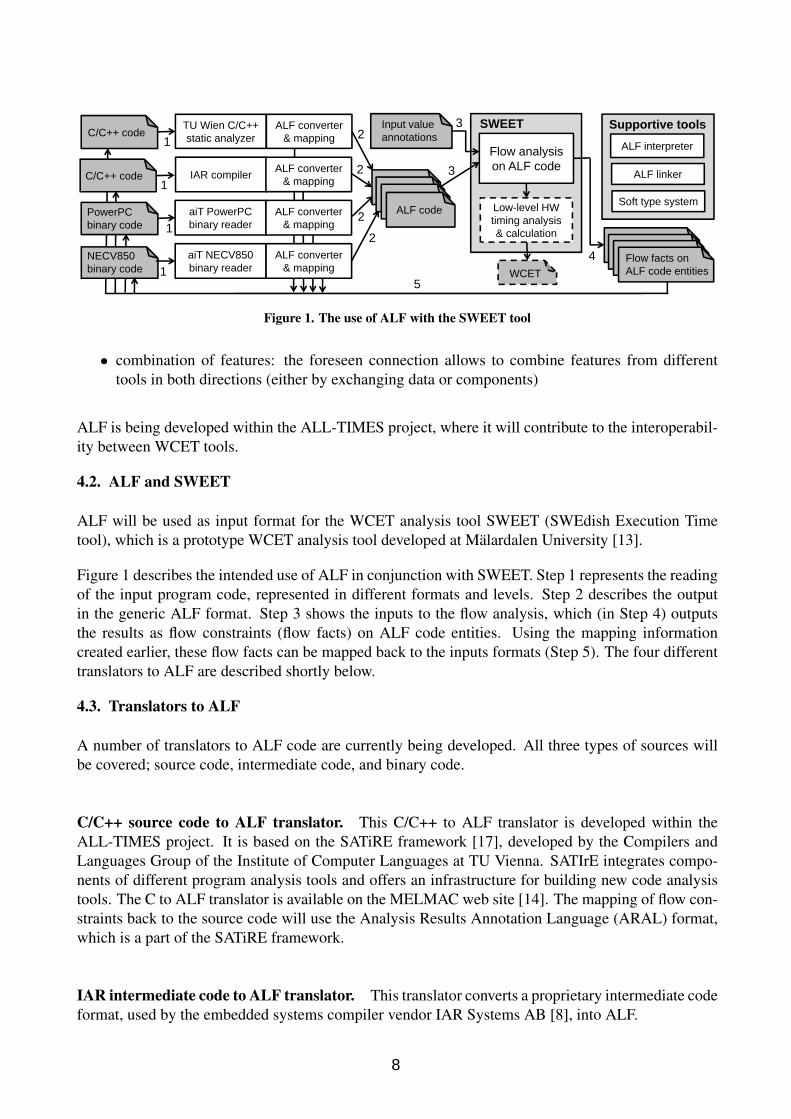
Figure 1. The use of ALF with the SWEET tool

• combination of features: the foreseen connection allows to combine features from differenttools in both directions (either by exchanging data or components)

ALF is being developed within the ALL-TIMES project, where it will contribute to the interoperabil-ity between WCET tools.

4.2. ALF and SWEET

ALF will be used as input format for the WCET analysis tool SWEET (SWEdish Execution Timetool), which is a prototype WCET analysis tool developed at Malardalen University [13].

Figure 1 describes the intended use of ALF in conjunction with SWEET. Step 1 represents the readingof the input program code, represented in different formats and levels. Step 2 describes the outputin the generic ALF format. Step 3 shows the inputs to the flow analysis, which (in Step 4) outputsthe results as flow constraints (flow facts) on ALF code entities. Using the mapping informationcreated earlier, these flow facts can be mapped back to the inputs formats (Step 5). The four differenttranslators to ALF are described shortly below.

4.3. Translators to ALF

A number of translators to ALF code are currently being developed. All three types of sources willbe covered; source code, intermediate code, and binary code.

C/C++ source code to ALF translator. This C/C++ to ALF translator is developed within theALL-TIMES project. It is based on the SATiRE framework [17], developed by the Compilers andLanguages Group of the Institute of Computer Languages at TU Vienna. SATIrE integrates compo-nents of different program analysis tools and offers an infrastructure for building new code analysistools. The C to ALF translator is available on the MELMAC web site [14]. The mapping of flow con-straints back to the source code will use the Analysis Results Annotation Language (ARAL) format,which is a part of the SATiRE framework.

IAR intermediate code to ALF translator. This translator converts a proprietary intermediate codeformat, used by the embedded systems compiler vendor IAR Systems AB [8], into ALF.

8

Binary code to ALF translators. Two binary translators are currently under development at Malar-dalen University, within the ALL-TIMES project. They translate CRL2 to ALF. CRL2 is a data formatmaintained by AbsInt GmbH [1], which is used by the aiT WCET analysis tool. CRL2 is mainly usedto represent various types of assembler code formats with associated analysis results. By using CRL2as source, the existing binary readers of aiT can be used to decode the binaries.

The first translator1 translates CRL2’s representation of NECV850E assembler code to ALF, and thesecond translator2 converts PowerPC code into ALF. To allow SWEET’s analysis results to be givenback to CRL2, a mapping between CRL2’s and ALF’s different code and data constructs will bemaintained. For both translators the generated flow constraints will be transferred to aiT using theAIS format, which is the annotation format used by aiT.

4.4. ALF interpreter

An ALF interpreter is currently being developed at Malardalen University3. The interpreter will beused for debugging ALF programs (or, indirectly, translators generating ALF), and other purposes.

4.5. ALF file linking

An embedded systems project may involve a variety of code sources, including code generated frommodelling tools, C or C++ code, or even assembler. To form a binary executable program, the sourcefiles are compiled and linked together with other object code files and libraries [11]. The latter areoften not available in source code format [15].

To handle this issue ALF must support the “linking” of several ALF files into one single ALF file.Since ALF is supposed to support reverse engineering of binaries and object code, it cannot have anadvanced module system with different namespaces. Instead ALF provides, similar to most objectcode formats [11], a set of exported symbols, i.e., lrefs or frefs visible to other ALF files, aswell as a set of symbols that must be imported, i.e., lrefs or frefs used but not declared in theALF file.

Forthcoming work includes the development of an ALF linker, i.e., a tool able to “link” ALF filesgenerated from many different code sources. It will here be interesting to see if it is also possibleto “link” (maybe partial) flow analysis results for individual ALF files to form a flow analysis resultvalid for the whole program.

5. Related Work

Generic intermediate languages have been used for other purposes. One example is the hardwaredescription language TDL [9] which was designed with the goal to generate machine-dependent post-pass optimizers and analyzers from a concise specification of the target processor. TDL provides ageneric modelling of irregular hardware constraints that are typical for many embedded processors.The part of TDL that is used to describe the semantics of instruction sets resembles ALF to somedegree.

1http://www.mdh.se/ide/eng/msc/index.php?choice=show&id=08752http://www.mdh.se/ide/eng/msc/index.php?choice=show&id=09173http://www.mdh.se/ide/eng/msc/index.php?choice=show&id=0830

9

6. Conclusions and Future Work

ALF can be seen as a step towards an open framework where flow analyses can be available andfreely used among several WCET analysis research groups and tool vendors. This framework willease the comparison of different flow analysis methods, and it will facilitate the future developmentof powerful flow analysis methods for WCET analysis tools.

There may be other uses for ALF than supporting flow analysis for WCET analysis tools. For instance,ALF can be used as a generic representation for different binary formats. Thus, very generic toolsfor analysis, manipulation, and reverse engineering of binary code may be possible to build usingALF. Possible examples include generic binary readers that reconstruct control flow graphs, and toolsthat can reconstruct arithmetics for long operators implemented using instruction sets for shorteroperators. The latter can be very useful when performing flow analysis for binaries compiled forsmall embedded processors, where the original arithmetics in the source code must be implementedusing an instruction set for short operators.

It would be simple to define an XML syntax for ALF. We might do so in the future, in order tofacilitate the use of standard tools for handling XML. Future work also includes further developmentof the PFF format for flow facts and the format for input value annotations.

Acknowledgment

This research was supported by the KK-foundation through grant 2005/0271, and the ALL-TIMESFP7 project, grant agreement no. 215068.

References

[1] ABSINT. aiT tool homepage, 2008. www.absint.com/ait.

[2] FERDINAND, C., HECKMANN, R., AND FRANZEN, B. Static memory and timing analysis of embedded systemscode. In 3rd European Symposium on Verification and Validation of Software Systems (VVSS’07), Eindhoven, TheNetherlands (Mar. 2007), no. TUE Computer Science Reports 07-04, pp. 153–163.

[3] GUSTAFSSON, J., ERMEDAHL, A., AND LISPER, B. ALF (ARTIST2 Language for Flow Analysis specification.Tech. rep., Malardalen University, Vasteras, Sweden, Jan. 2009.

[4] GUSTAFSSON, J., LISPER, B., SANDBERG, C., AND BERMUDO, N. A tool for automatic flow analysis ofC-programs for WCET calculation. In Proc. 8th IEEE International Workshop on Object-oriented Real-time De-pendable Systems (WORDS 2003) (Jan. 2003).

[5] GUSTAFSSON, J., LISPER, B., SCHORDAN, M., FERDINAND, C., GLIWA, P., JERSAK, M., AND BERNAT,G. ALL-TIMES - a European project on integrating timing technology. In Proc. 3rd International Symposium onLeveraging Applications of Formal Methods (ISOLA’08) (Porto Sani, Greece, Oct. 2008), vol. 17 of CCIS, Springer,pp. 445–459.

[6] HOLSTI, N. Analysing switch-case tables by partial evaluation. In Proc. 7th International Workshop on Worst-CaseExecution Time Analysis (WCET’2007) (2007).

[7] HOLSTI, N., AND SAARINEN, S. Status of the Bound-T WCET tool. In Proc. 2nd International Workshop onWorst-Case Execution Time Analysis (WCET’2002) (2002).

[8] IAR Systems homepage.URL: http://www.iar.com.

[9] KASTNER, D. TDL: A hardware description language for retargetable postpass optimizations and analyses. InProc. 2nd International Conference on Generative Programming and Component Engineering (GPCE’03), LectureNotes in Computer Science (LNCS) 2830. Springer-Verlag, 2003.

10

[10] KIRNER, R. Extending Optimising Compilation to Support Worst-Case Execution Time Analysis. PhD thesis,Technische Universitat Wien, Treitlstr. 3/3/182-1, 1040 Vienna, Austria, May 2003.

[11] LEVINE, J. Linkers and Loaders. Morgan Kaufmann, 2000. ISBN 1-55860-496-0.

[12] LISPER, B. Fully automatic, parametric worst-case execution time analysis. In Proc. 3rd International Workshopon Worst-Case Execution Time Analysis (WCET’2003) (Porto, July 2003), J. Gustafsson, Ed., pp. 77–80.

[13] MALARDALEN UNIVERSITY. WCET project homepage, 2008. www.mrtc.mdh.se/projects/wcet.

[14] MELMAC. MELMAC homepage, 2009.http://www.complang.tuwien.ac.at/gergo/melmac.

[15] MONTAG, P., GOERZIG, S., AND LEVI, P. Challenges of timing verification tools in the automotive domain. InProc. 2nd International Symposium on Leveraging Applications of Formal Methods (ISOLA’06) (Paphos, Cyprus,Nov. 2006), T. Margaria, A. Philippou, and B. Steffen, Eds.

[16] PRANTL, A., SCHORDAN, M., AND KNOOP, J. TuBound – A Conceptually New Tool for Worst-Case ExecutionTime Analysis. In Proc. 8th International Workshop on Worst-Case Execution Time Analysis (WCET’2008) (Prague,Czech Republic, July 2008), R. Kirner, Ed., pp. 141–148.

[17] SATIRE. SATIrE homepage, 2009.http://www.complang.tuwien.ac.at/markus/satire.

[18] SEHLBERG, D., ERMEDAHL, A., GUSTAFSSON, J., LISPER, B., AND WIEGRATZ, S. Static WCET analysisof real-time task-oriented code in vehicle control systems. In Proc. 2nd International Symposium on LeveragingApplications of Formal Methods (ISOLA’06) (Paphos, Cyprus, Nov. 2006), T. Margaria, A. Philippou, and B. Steffen,Eds.

[19] THEILING, H. Control Flow Graphs For Real-Time Systems Analysis. PhD thesis, University of Saarland, 2002.

[20] WRIGHT, A. K., AND CARTWRIGHT, R. A practical soft type system for scheme. ACM Trans. Program. Lang.Syst. 19, 1 (Jan. 1997), 87–152.

11

SOURCE-LEVEL WORST-CASE TIMINGESTIMATION AND ARCHITECTURE

EXPLORATION IN EARLY DESIGN PHASES

Stefana Nenova and Daniel Kastner 1

AbstractSelecting the right computing hardware and configuration at the beginning of an industrial projectis an important and highly risky task, which is usually done without much tool support, based onexperience gathered from previous projects. We present TimingExplorer - a tool to assist in the ex-ploration of alternative system configurations in early design phases. It is based on AbsInt’s aiTWCET Analyzer and provides a parameterizable core that represents a typical architecture of inter-est. TimingExplorer requires (representative) source code and enables its user to take an informeddecision which processor configurations are best suited for his/her needs. A suite of TimingExplorerswill facilitate the process of determining what processors to use and it will reduce the risk of timingproblems becoming obvious only late in the development cycle and leading to a redesign of largeparts of the system.

1. Introduction

Choosing a suitable processor configuration (core, memory, peripherals, etc.) for an automotiveproject at the beginning of the development is a challenge. In the high-volume market, choosinga too powerful configuration can lead to a serious waste of money. Choosing a configuration notpowerful enough leads to severe changes late in the development cycle and might delay the delivery.

Currently to a great extent this risky decision is taken based on gut feeling and previous experience.The existing timing analysis techniques require executable code as well as a detailed model of thetarget processor for static analysis or actual hardware for measurements. This means that they can beapplied only relatively late in the design, when code and hardware (models) are already far developed.Yet timing problems becoming apparent only in late design stages may require a costly re-iterationthrough earlier stages. Thus, we are striving for the possibility to perform timing analysis already inearly design stages.

Existing techniques that are applicable at this stage include performance estimation and simulation(e.g., virtual system prototypes, instruction set simulators, etc. ). It should be noted that these ap-proaches use manually created test cases and therefore only offer partial coverage. As a result, cornercases that might lead to timing problems can easily be missed. Since we follow a completely differentapproach, we will not further review existing work in these areas.

Our goal is to provide a family of tools to assist in the exploration of alternative system configurationsbefore committing to a specific solution. They should perform an automatic analysis, be efficientand provide 100% coverage on the analyzed software so that critical corner cases are automatically

1AbsInt Angewandte Informatik GmbH, Science Park 1, D-66123 Saarbrucken, Germany

12

considered. Using these tools, developers will be able to answer questions like “what would happen ifI take a core like the ABCxxxx and add a small cache and a scratchpad memory in which I allocate theC-stack or a larger cache” or “what would be the overall effect of having an additional wait cycle ifI choose a less expensive flash module”, . . . Such tools can be of enormous help when dimensioninghardware and will reduce the risk of a project delay due to timing issues.

The paper is structured as follows. We describe how TimingExplorer is to be used in Section 2. InSection 3 we present AbsInt’s aiT WCET Analyzer and compare it to TimingExplorer in Section 4.Finally we discuss a potential integration of TimingExplorer in a system-level architecture explorationanalysis in Section 5.

2. TimingExplorer Usage

In the early stage of an automotive project it has to be decided what processor configuration is bestsuited for the application. The ideal architecture is as cheap as possible, yet powerful enough so thatall tasks can meet their deadlines. There are usually several processor cores that come into question,as well as a number of possible configurations for memory and peripherals. How do we choose theone with the right performance?

Our approach requires that (representative) source code of (representative) parts of the application isavailable. This code can come from previous releases of a product or can be generated from a modelwithin a rapid prototyping development environment.

The way to proceed is as follows. The available source code is compiled and linked for each of thecores in question. In the case one uses a model-based design tool with an automatic code generator,this step corresponds to launching the suitable code generator on the model. Each resulting executableis then analyzed with the TimingExplorer for the corresponding core. The user has the possibility tospecify memory layout and cache properties. The result of the analysis is an estimation of the WCETfor each of the analyzed tasks given the processor configuration. To see how the tasks will behave onthe same core, but with different memory layout, memory or cache properties, one simply has to rerunthe analysis with the appropriate description of cache and memory. Finally, the estimated executiontimes can be compared and the most appropriate configuration can be chosen.

Let us consider three tasks that come from a previous release of the system. Having an idea ofthe behavior of the old version of the system and the extensions we want to add to it in the newversion, we wonder whether a MPC565 core will be sufficient for the project or it is better to use themore powerful MPC5554 core that offers more memory and cache and a larger instruction set. Thissituation is depicted in Figure 1. The tools we need are TimingExplorer for MPC5xx (TE5xx) andTimingExplorer for MPC55xx (TE55xx) for assessing the timing behavior of the tasks on the MPC565and MPC5554 core respectively. First we compile and link the sources for MPC5xx and MPC55xx,which results in the executables E5xx and E55xx. Then we write the configuration files C5xx andC55xx to describe the memory layout, the memory timing properties and the cache parameters whenapplicable for the configurations in question. Next we analyze each of the tasks T1, T2 and T3 for eachof the two configurations. To get an estimate for the WCET of the tasks on the MPC5554 core, we runTE55xx with inputs E55xx and C55xx for each of the tasks. We proceed similarly to obtain an estimateof the timing for the tasks on the MPC565 core. By comparing the resulting times (X1, X2, X3) and(Y1, Y2, Y3), we see that the speed and resources provided by the MPC565 core will not be sufficientfor our needs, so we settle for the MPC5554 core.

13

Figure 1. Usage of TimingExplorer to choose a suitable core

Figure 2. Usage of TimingExplorer to choose a suitable cache and memory configuration

The next step is to choose the cache and memory parameters. The core comes with 32KB cache,64KB SRAM and 2MB Flash and gives the possibility to turn off caching and configure part of the32KB of cache as additional RAM. We want to know what is more beneficial for our application – tohave more memory or use caching. The situation is depicted in Figure 2. We write two configurationfiles: Ccache, in which we use the cache as such, and Cram, in which we use it as RAM where weallocate the C stack space that usually shows a high degree of reuse. To see how the tasks run on asystem with cache, we run TE55xx with inputs E55xx and Ccache. To assess the performance withoutthe use of cache, we run TE55xx with inputs E55xx and Cram. Based on the analysis results we candecide with more confidence which of the hardware configurations to choose.

An important question is how the choice of a compiler affects the results. Opposed to some existingsimulation techniques that work solely on the source-code level and completely ignore the effect thecompiler has on the program’s performance, both aiT and TimingExplorer operate on the binary exe-cutable and are thus able to achieve high precision. Ideally during the architecture exploration phasethe user has the compiler that would be used in the final project at his disposal (for instance becauseit has been used to build the previous version of the system). Using the actual compiler to obtain anexecutable is the best way to obtain precise estimates. However when using the production compileris impossible for some reasons, an executable compiled with a different compiler can be used for theanalysis. A preferable solution in this case is to use a compiler that is available for all configurationsunder consideration. In the examples discussed above we could use gcc for MPC5xx and MPC55xxto obtain E5xx and E55xx respectively. The goal of TimingExplorer is to assess hardware effects onthe same code. The observed effects can be expected to also hold when the production compilers arenot used provided that the same or at least comparable optimization settings are used.

14

Figure 3. Phases of WCET computation

3. aiT WCET Analyzer

aiT WCET analyzer [7] automatically computes tight upper bounds of worst-case execution times oftasks in real-time systems, a task in this context being a sequentially executed piece of code withoutparallelism, interrupts, etc. As an input, the tool takes a binary executable together with the startaddress of the task to be analyzed. In addition, it may be provided with supplementary informationin the form of user annotations. Through annotations the user provides information aiT needs tosuccessfully carry out the analysis or to improve precision. Such information may include boundson loop iterations and recursion depths that cannot be determined automatically, targets of computedcalls or branches, description of the memory layout, etc. The result of the analysis is a bound of theWCET of the task as well as a graphical visualization of the call graph in which the WCET path ismarked in red.

Due to the use of caches, pipelines and speculation techniques in modern microcontrollers to improvethe performance, the execution time of an individual instruction can vary significantly depending onthe execution history. Therefore aiT precisely models the cache and pipeline behavior and takes theminto account when computing the WCET bound. In our approach [8] the analysis is performed inseveral consecutive phases (see Figure 3):

1. CFG Building: decoding and reconstruction of the control-flow graph from a binary pro-gram [20];

2. Value Analysis: computation of value ranges for the contents of registers and address ranges forinstructions accessing memory;

3. Loop Bound Analysis: determination of upper bounds for the number of iterations of simpleloops;

4. Cache Analysis: classification of memory references as cache misses or hits [6];

15

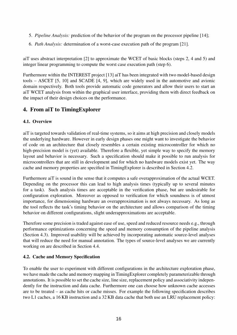
5. Pipeline Analysis: prediction of the behavior of the program on the processor pipeline [14];

6. Path Analysis: determination of a worst-case execution path of the program [21].

aiT uses abstract interpretation [2] to approximate the WCET of basic blocks (steps 2, 4 and 5) andinteger linear programming to compute the worst case execution path (step 6).

Furthermore within the INTEREST project [13] aiT has been integrated with two model-based designtools – ASCET [5, 10] and SCADE [4, 9], which are widely used in the automotive and avionicdomain respectively. Both tools provide automatic code generators and allow their users to start anaiT WCET analysis from within the graphical user interface, providing them with direct feedback onthe impact of their design choices on the performance.

4. From aiT to TimingExplorer

4.1. Overview

aiT is targeted towards validation of real-time systems, so it aims at high precision and closely modelsthe underlying hardware. However in early design phases one might want to investigate the behaviorof code on an architecture that closely resembles a certain existing microcontroller for which nohigh-precision model is (yet) available. Therefore a flexible, yet simple way to specify the memorylayout and behavior is necessary. Such a specification should make it possible to run analysis formicrocontrollers that are still in development and for which no hardware models exist yet. The waycache and memory properties are specified in TimingExplorer is described in Section 4.2.

Furthermore aiT is sound in the sense that it computes a safe overapproximation of the actual WCET.Depending on the processor this can lead to high analysis times (typically up to several minutesfor a task). Such analysis times are acceptable in the verification phase, but are undesirable forconfiguration exploration. Moreover as opposed to verification for which soundness is of utmostimportance, for dimensioning hardware an overapproximation is not always necessary. As long asthe tool reflects the task’s timing behavior on the architecture and allows comparison of the timingbehavior on different configurations, slight underapproximations are acceptable.

Therefore some precision is traded against ease of use, speed and reduced resource needs e.g., throughperformance optimizations concerning the speed and memory consumption of the pipeline analysis(Section 4.3). Improved usability will be achieved by incorporating automatic source-level analysesthat will reduce the need for manual annotation. The types of source-level analyses we are currentlyworking on are described in Section 4.4.

4.2. Cache and Memory Specification

To enable the user to experiment with different configurations in the architecture exploration phase,we have made the cache and memory mapping in TimingExplorer completely parameterizable throughannotations. It is possible to set the cache size, line size, replacement policy and associativity indepen-dently for the instruction and data cache. Furthermore one can choose how unknown cache accessesare to be treated – as cache hits or cache misses. For example the following specification describestwo L1 caches, a 16 KB instruction and a 32 KB data cache that both use an LRU replacement policy:

16

cache instructionset-count = 128, assoc = 4, line-size = 32,policy = LRU, may = empty

and dataset-count = 256, assoc = 4, line-size = 32,policy = LRU, may = empty;

With respect to the memory map, one can specify memory areas and their properties. A memory areais specified as an address range. Useful properties include the time it takes to read and write data tothe area, whether write accesses are allowed or the area is read-only, if accesses are cached, etc.

4.3. Pipeline Analysis

To speed up the analysis and reduce memory needs TimingExplorer uses parametric pipeline analysisand computes local rather than global worst-case time as done by aiT. The difference between thelatter two kinds of computations is what the tool does when the abstract cache and pipeline state isabout to fork into two or more successor states because of imprecise information. This happens forinstance when a memory access cannot be classified as cache hit or cache miss. In the case of globalworst-case, the tool creates all successor states and follows their further evolution. In contrast, localworst-case means that it immediately decides which successor is likely to be the worst, and onlyfollows the evolution of this single state.

For example, consider that we have two consecutive unclassified memory accesses a1 and a2 and lethi denote the case when ai is a cache hit and mi when it is a cache miss. aiT uses global worst-case computation, so after the first unclassified access it creates the superstate {(h1) , (m1)} and afterthe second – the superstate {(h1, h2) , (h1, m2) , (m1, h2) , (m1, m2)}. From that point on it performsevery computation for each of the four concrete states. At the end it compares the resulting times andchooses the highest one. Due to timing anomalies it is not necessary that the worst case is the oneresulting from the state (m1, m2).

On the other hand TimingExplorer uses local worst-case computation. Unless anything else is speci-fied, this means that a memory access takes longer to execute if it is a cache miss. Therefore after thefirst unknown access TimingExplorer will simply assume that it is a cache miss and create the state(m1) and after the second the state (m1, m2). It proceeds the execution with a single state (and notwith a superstate like aiT).

It should be noted that because of the local worst-case computation the result is not necessarily anoverapproximation of the WCET. It is sound in the case of fully timing compositional architecturesi.e. architectures without timing anomalies [22], but can be an underestimate otherwise. However theuse of local worst case may drastically improve the performance in the cases when there are frequentpipeline state splits.

4.4. Source-code Analyses

4.4.1. Overview

To successfully analyze a task, aiT and TimingExplorer need information about the number of loopiterations, recursion bounds, targets of computed calls and branches. Partially such information can

17

be automatically discovered when analyzing the binary, e.g., the loop bound analysis mentioned inSection 3 can discover bounds for the number of iterations of simple loops. However information thatcannot be discovered automatically has to be supplied to the tool in the form of annotations. To reducethe need of manual annotation, source level analysis will be incorporated that will try to determineauxiliary information that TimingExplorer can extract from the executable.

It should be noted that due to compiler optimizations, the information extracted from the source codedoes not necessarily correspond to the behavior of the executable. Consider the loop

for (int i=0; i<100; i++)...

The compiler could discover that the loop will be executed at least once and move the exit conditionfrom the header to the bottom, turning it into a do/while loop. Doing so it reduces the number ofjumps by two, which can improve the performance, since jumps often cause a pipeline stall. Fur-thermore the test condition will be evaluated 100 times (and not 101 times as we will discover bysource-level analysis). The resulting overapproximation will result in some precision loss. Whereasin a verification phase the analysis precision is of utmost importance and any loss of precision isundesirable, in an exploration configuration stage the overapproximation is often acceptable becauseof the time and effort gain from reducing the manual annotation process. Furthermore, the resultsof the source-level analyses are independent of the compiler and the target architecture and thereforethe resulting precision losts will be the same for each of the analyzed configurations. Thus despitethe possible overapproximation introduced by incorporating source-level analyses, the comparison ofdifferent configurations will still be precise.

Currently, we are working on source level analyses for extracting loop bounds [12] and targets offunction calls when function pointers are used [18]. Both of these analyses are implemented withhelp of the SATIrE framework [17], the LLNL-ROSE compiler [15] and PAG [16].

4.4.2. Function-pointer Analysis

The use of function pointers makes the static analysis of a program hard, because in the general caseit cannot be determined which functions will be called at runtime. This leads to an imprecise controlflow graph and therefore imprecise results. Unfortunately function pointers are quite common inautomotive software and manual annotation should be avoided, because it can be cumbersome anderror-prone. Therefore we plan to integrate an automatic analysis for function pointer resolution.

For each function pointer variable in the program the analysis computes a points-to set containingall memory locations whose address might be stored in the variable. The analysis information isstored in a recursive fashion thus making it easy to handle function pointers that are stored withinarbitrarily complex objects, like structures with arrays of function pointers. As an output the analysiscan create annotations for TimingExplorer, which will relieve the user from determining targets offunction pointer calls manually.

During our experiments we were able to successfully analyze several medium-sized C programs. Anoverview of our test suite is given in Table 1. For the programs in this suite, the analysis detectedall function pointers and a manual inspection of the results gave the impression, that they were closeto an optimal solution. Our first attempts to analyze real automotive software were not successful,

18

Program Version Lines of code Indirect callsdiction 0.7 2 037 3grep 2.0 12 417 3gzip 1.2.4 8 163 4sim6890 0.1 3 290 97

Table 1. Test suite for the source-level analysis of function pointers

primarily because of problems in LLNL-ROSE and SATIrE. In some cases this was caused by theuse of special language keywords, since the projects had been developed using compilers for targetarchitectures with small word size and used special language constructs. Unfortunately SATIrE alsohad problems with certain C-constructs (e.g., valid source made it crash).

4.4.3. Loop-bound Analysis

In the case of loop bound analysis we express the upper loop bound as a parametric formula dependingon parameters – variables and expressions that are constant within the loop. The symbolic formula isconstructed once for each loop in an analysis run that precedes the rest of the analyses. Afterwardsas soon as the value analysis obtains bounds on the values of all the parameters in a certain formula,a concrete bound on the loop iteration count for that case can be computed with low computationaleffort.

In an initial evaluation phase we used the Malardalen WCET benchmark suite [23] to compare ouranalysis to oRange [1] and the loop bound analysis component in SWEET [3]. The tests showed that:

• The analysis detects and assigns a loop bound to all loops established with C loop constructsexcept for the cases of loops inside recursive functions or when LLNL-ROSE and SATIrE meetunsupported constructs.

• The precision of the computed loop bounds (assuming that precise values of parameters areprovided by an external value analysis) is higher than the one of SWEET and in most caseshigher or equal to the precision of oRange.

• The analysis can cope with automatically generated code.

• The analysis is especially effective for typical counter-based loops, which are common in gen-erated code.

Therefore we believe that incorporating source-level loop-bound analysis in TimingExplorer willdrastically reduce the number of loops that have to be annotated manually. In the case, when evenafter the automatic analysis some loop bounds are unknown and the user does not want to spend timeon specifying their bounds manually, we have foreseen the possibility to give a global default boundto all loops of unknown iteration count.

5. Integration in a System-level Analysis

After incorporating the source-code level analyses discussed in the previous section in TimingEx-plorer, we will have a tool capable of predicting the WCET of a task on a selected target architecture

19

Figure 4. Flow of requests and responses between aiT and SymTA/S

almost automatically. Yet as presented so far, the tool will work only for single tasks without inter-rupts or exceptions. On the other hand, schedulability analyzers can determine the overall worst-caseresponse time of a system provided the corresponding results for single tasks are known.

Within the European FP6 STREP Project INTEREST [13], a generic information exchange formatcalled XML Timing Cookies (XTC) has been developed. With its help, users of a scheduling analysistool can cause aiT to perform timing analyses at the code level, whose results are mapped back tothe scheduling tool in a fully automatic way. In particular a coupling of aiT with SymTA/S has beenrealized (Figure 4).

SymTA/S [11, 19] of Symtavision GmbH is a modular tool-suite for scheduling analysis and op-timization for electronic controllers, buses/networks and complete embedded real-time systems. Itcomputes the worst-case response times of tasks and the worst-case end-to-end communication de-lays taking into account the WCETs of the tasks, scheduling, bus arbitration, possible interrupts andtheir priorities. Two SymTA/S modules that are of special interest for architecture exploration are theSensitivity Analysis and Design-Space Exploration. The Sensitivity Analysis module allows its userto determine the robustness of a system and its extensibility for future functions. With the help ofthe Design-Space Exploration plug-in one can evaluate alternative system configurations and performsystem optimization. One specifies which system parameters can be varied and defines optimizationobjectives, and the tool presents him the most interesting alternatives and the corresponding trade-offs.

We plan to use XTC and integrate TimingExplorer into the SymTA/S system-level architecture ex-ploration analysis. After such integration an overall timing analysis can be performed that will allowusers to assess how much room there is for estimation errors and how much flexibility remains forlater changes. The combination of code-level and system-level architecture exploration will lead toinformed decisions with respect to which architectures are appropriate for an application.

6. Conclusion

We have presented TimingExplorer – a source-level worst-case timing estimation tool to assist inthe exploration of alternative system configurations in early design phases. It is an extension of

20

AbsInt’s aiT WCET Analyzer, provides a flexible way to specify an architecture of interest and yieldsprecise estimates of the time it will take a task to run on the modelled architecture. FurthermoreTimingExplorer takes all program executions on all inputs into account so that critical corner casesare automatically considered.

We gave an example how a suite of TimingExplorers is to be used to decide what architecture touse for a project and explained the way TimingExplorer differs from aiT. We described two types ofsource-code analyses that we want to incorporate in TimingExplorer to minimize the need for manualannotation. We also suggested a way to integrate the tool in a system-level exploration framework sothat the overall timing performance of the system can be estimated.

We believe that a suite of TimingExplorers will considerably facilitate the process of dimensioninghardware at the beginning of a project. It will allow system architects to assess performance con-siderations, such as processor capacity, memory layout, cache sizing etc. Thus when choosing whatconfiguration to use they will no longer rely solely on experience and intuition as they do now, butwill have an estimate of how the software will behave on the selected architecture at hand.

7. Acknowledgements

This work has partially been supported by the research project “Integrating European Timing Anal-ysis Technology” (ALL-TIMES) under contract No 215068 funded by the 7th EU R&D FrameworkProgram.

References

[1] CASSE, H., DE MICHIEL, M., BONENFANT, A., AND SAINRAT, P. Static Loop Bound Analysis ofC Programs Based on Flow Analysis and Abstract Interpretation. In Proceedings of the 14th IEEE Con-ference on Embedded and Real-Time Computing Systems and Applications (RTCSA 2008) (Kaohsiung,Taiwan, 2008).

[2] COUSOT, P., AND COUSOT, R. Abstract Interpreatation: A Unified Lattice Model for Static Analysisof Programs by Construction or Approximation of Fixpoints. In Proceedings of the 4th ACM Symposiumon Principles of Programming Languages (POPL 1977) (Los Angeles, California, 1977).

[3] ERMEDAHL, A., SANDBERG, C., GUSTAFSSON, J., BYGDE, S., AND LISPER, B. Loop boundanalysis based on a combination of program slicing, abstract interpretation, and invariant analysis. InProceedings of the 7th International Workshop on Worst-Case Execution Time Analysis (WCET 2007)(Pisa, Italy, 2007).

[4] Esterel Technologies. SCADE Suite. http://esterel-technologies.com/products/scade-suite.

[5] ETAS Group. ASCET Software Products. http://www.etas.com/en/products/ascet_software_products.php.

[6] FERDINAND, C. Cache Behavior Prediction for Real-Time Systems. PhD thesis, Saarland University,1997.

[7] FERDINAND, C., AND HECKMANN, R. aiT: Worst-Case Execution Time Prediction by Static Pro-gramm Analysis. In Building the Information Society. IFIP 18th World Computer Congress, TopicalSessions. Toulouse, France, 2004, pp. 377–384.

21

[8] FERDINAND, C., HECKMANN, R., LANGENBACH, M., MARTIN, F., SCHMIDT, M., THEILING,H., THESING, S., AND WILHELM, R. Reliable and precise WCET determination for a real-life pro-cessor. In Proceedings of the First Workshop on Embedded Software (EMSOFT 2001) (Tahoe City, CA,USA, 2001), vol. 2211 of Lecture Notes in Computer Science, Springer-Verlag.

[9] FERDINAND, C., HECKMANN, R., LE SERGENT, T., LOPES, D., MARTIN, B., FORNARI, X., ANDMARTIN, F. Combining a high-level design tool for safety-critical systems with a tool for WCET analysison executables. In Proceedings of the 4th European Congress Embedded Real Time Software (ERTS 2008)(Toulouse, France, 2008).

[10] FERDINAND, C., HECKMANN, R., WOLFF, H.-J., RENZ, C., GUPTA, M., PARSHIN, O., AND WIL-HELM, R. Towards integrating model-driven development of hard real-time systems with static programanalyzers. In SAE 2007 (Detroit, USA).

[11] HENIA, R., HAMANN, A., JERSAK, M., RACU, R., RICHTER, K., AND ERNST, R. System levelperformance analysis – the SymTA/S approach. In IEEE Proceedings Computers and Digital Techniques(2005), vol. 152.

[12] HONCHAROVA, O. Static Detection of Parametric Loop Bounds on C Code. Master’s thesis, SaarlandUniversity, 2009.

[13] INTEREST project. http://www.interest-strep.eu.

[14] LANGENBACH, M., THESING, S., AND HECKMANN, R. Pipeline modeling for timing analysis.In Proceedings of the 9th International Static Analysis Symposium (SAS 2002) (Madrid, Spain, 2002),vol. 2477 of Lecture Notes in Computer Science, Springer-Verlag.

[15] LLNL-ROSE. http://rosecompiler.de.

[16] MARTIN, F. Generation of Program Analyzers. PhD thesis, Saarland University, 1999.

[17] SCHORDAN, M. Combining tools and languages for static analysis and optimization of high-level ab-stractions. Tech. rep., TU Vienna, Austria, 2007.

[18] STATTELMANN, S. Function Pointer Analysis for C Programs. Bachelor’s thesis, Saarland University,2008.

[19] Symtavision. SymTA/S. http://www.symtavision.com/symtas.html.

[20] THEILING, H. Extracting Safe and Precise Control Flow from Binaries. In Proceedings of the 7thConference on Real-Time Computing and Applications Symposium (RTCSA 2000) (Cheju Island, SouthKorea, 2000), IEEE Computer Society.

[21] THEILING, H., AND FERDINAND, C. Combining abstract interpretation and ILP for microarchitecturemodelling and program path analysis. In Proceedings of the 19th IEEE Real-Time Systems Symposium(RTSS 1998) (Madrid, Spain, 1998).

[22] THIELE, L., AND WILHELM, R. Design for timing predictability. Real-Time Systems 28, 2-3 (2004),157–177.

[23] WCET benchmarks project. http://www.mrtc.mdh.se/projects/wcet.

22

COMPARISON OF IMPLICIT PATHENUMERATION AND MODEL CHECKING

BASED WCET ANALYSIS

Benedikt Huber and Martin Schoeberl1

AbstractIn this paper, we present our new worst-case execution time (WCET) analysis tool for Java processors,supporting both implicit path enumeration (IPET) and model checking based execution time estima-tion. Even though model checking is significantly more expensive than IPET, it simplifies accuratemodeling of pipelines and caches. Experimental results using the UPPAAL model checker indicate thatmodel checking is fast enough for typical tasks in embedded applications, though large loop boundsmay lead to long analysis times. To obtain a tool which is able to cope with larger applications, werecommend to use model checking for more important code fragments, and combine it with the IPETapproach.

1. Introduction

Worst-case execution time (WCET) analysis is needed as input to schedulability analysis. As mea-suring the WCET is not a safe approach, real-time tasks have to be analyzed statically. We presenta WCET analysis tool for Java. The first target processor that is supported by the tool is the Javaprocessor JOP [24]. A future version will also support the multi-threaded Java processor jamuth [27].

The WCET analysis is performed on Java bytecodes, the intermediate representation of compiled Javaprograms. A Java virtual machine (JVM) executes bytecodes by either interpreting the bytecodes,compiling them to native code, or executing them in hardware. The latter case is the execution modelof a Java processor. Using bytecode as the instruction set without further transformation simplifiesWCET analysis, as the execution time can be modeled at the bytecode level.

The primary method for estimating the WCET is based on the standard IPET approach [21]. Wehave implemented a context sensitive, bottom-up analysis, and an interprocedural analysis to supporta simple method cache approximation. The tool additionally targets the UPPAAL model checker [3].The control flow graphs (CFG) are modeled as timed automata, and a binary search is used to obtainthe WCET. An (exact) cache simulation was added to the UPPAAL model, which is used to evaluatethe quality of static cache approximations. Having implemented those two methods in a single tool,we compare traditional IPET with model checking based techniques.

Although we analyze Java programs, neither the model checking based analysis nor the method cacheare Java specific (e.g., the method cache has been implemented in the CarCore processor [15]).

1Institute of Computer Engineering, Vienna University of Technology, Austria;email: benedikt.huber@student.tuwien.ac.at, mschoebe@mail.tuwien.ac.at

23

1.1. The Target Architecture JOP

JOP [24] is an implementation of the Java virtual machine (JVM) in hardware. The design is opti-mized for low and predictable WCETs. Advanced features, such as branch prediction or out-of-orderexecution, that are hard to model for the WCET analysis, are completely avoided. Instead, the pipelineand the caches are designed to deliver good real-time performance.

Caches are a mandatory feature for pipelined architectures to feed the pipeline with enough instruc-tions and speedup load/store instructions. Although direct-mapped caches or set-associative cacheswith a least recently used (LRU) replacement policy are WCET friendly, the instruction cache in JOPhas a different organization. The cache stores full methods and is therefore named method cache [23].The major benefit of that cache is that cache misses can only occur at method invoke or on a returnfrom a method. All other instructions are guaranteed hits and the cache can be ignored during WCETanalysis.

JOP uses a variable block method cache, where methods are allowed to occupy more than one cacheblock. JOP currently implements the variable block cache using a so called next-block replacement,effectively a first in, first out (FIFO) strategy. It is known, that the FIFO replacement strategy is notideal for WCET analysis [22]. A LRU replacement would be preferable, as it provides a better cachingbehavior and is easier to analyze. However, the constraint on the method cache that a method has tospan several contiguous blocks, makes the implementation of a LRU replacement strategy difficult.

1.2. Related Work

WCET related research started with the introduction of timing schemas by Shaw [26]. Shaw presentsrules to collapse the CFG of a program until a final single value represents the WCET. An overviewof actual WCET research can be found in [20, 28]. Computing the WCET with an integer linearprogramming solver is proposed in [21] and [13]. The approach is named graph-based and implicitpath enumeration respectively. We base our WCET analyzer on the ideas from these two groups.

Cache memories for the instructions and data are classic examples of the paradigm: Make the commoncase fast. Avoiding or ignoring this feature in real-time systems, due to its unpredictable behavior,results in a very pessimistic WCET bound. Plenty of effort has gone into research to integrate the in-struction cache into the timing analysis of tasks [1, 9] and cache analysis integration with the pipelineanalysis [8]. Heckmann et. al described the influence of different cache architectures on WCET anal-ysis [10]. Our approach to cache analysis is to simplify the cache with the method cache. Thatform of caching needs no integration with the pipeline analysis and the hit/miss categorization can beapproximated at the call graph, which leads to shorter analysis times.

WCET analysis at the bytecode level was first considered in [4]. It is argued that the well formedintermediate representation of a program, the Java bytecode, is well suited for a portable WCET anal-ysis tool. In that paper, annotations for Java and Ada are presented to guide the WCET analysis atbytecode level. The work is extended in [2] to address the machine-dependent low-level timing anal-ysis. Worst-case execution frequencies of Java bytecodes are introduced for a machine independenttiming information. Pipeline effects (on the target machine) across bytecode boundaries are modeledby a gain time for bytecode pairs. Due to our target architecture that executes Java bytecode nativelywe can extend on the work of WCET analysis at bytecode level.

24

In [25], an IPET based WCET analysis tool is presented that includes the timing model of JOP. Asimplified version of the method cache, the two block cache, is analyzed for invocations in innerloops. Trevor Harmon developed a tree-based WCET analyzer for interactive back-annotation ofWCET estimates into the program source [6]. The tool is extended to integrate JOP’s method cache [7]in a similar way as in [25]. Compared to those two tools, which also target JOP, our presented WCETtool is enhanced with: (a) analysis of bytecodes that are implemented in Java; (b) a tighter methodcache analysis; and (c) an evaluation of model checking for WCET analysis and exact modeling ofthe method cache in the model checking approach.

Whether and to what extend model checking can deliver tighter WCET bounds than IPET is inves-tigated in [16]. Though we use timed automata and a different cache model, the argument that stateexploration is potentially more precise than IPET still applies. A project closely related to our modelchecking approach is presented in [5]. Model checking of timed automata is used to verify the schedu-lability of a complete application. However, even with a simple example, consisting of two periodicand two sporadic tasks, this approach leads to a very long analysis time.

2. The WCET Analysis Tool

The new WCET analysis tool deals with a less restricted subset of Java than [25], adding support forbytecodes implemented in Java and dynamic dispatch. The supported subset of the Java languageis restricted to acyclic callgraphs. As any static WCET analysis, we require the set of classes to beknown at compile time.

For determining loop bounds, we rely on both source code annotations (similar to the ones describedin [11, 25]) and dataflow analysis [19]. The latter is also used for computing the set of methodspossibly executed when a virtual method is invoked. By default, the WCET is calculated using IPET,taking the variable block method cache into account (see Section 2.1.). Additionally, a translation totimed automata has been implemented, including method cache simulations (see Section 2.2.).

2.1. IPET and Static Cache Approximation

The primary method for estimating the WCET is based on the standard IPET approach [21]. Hereby,the WCET is computed by solving a maximum cost circulation problem in a directed graph repre-senting the program’s control flow. Each edge is associated with a certain cost for executing it, andlinear constraints are used to exclude infeasible paths.

In addition to the usual approach modeling the application as one big integer linear program (ILP), wealso support a bottom-up analysis, which first analyses referenced methods separately and then solvesthe intraprocedural ILP model. This is a fast, simple alternative to the global model, and allows us toinvoke the model checker for smaller, important parts of the application. Furthermore, the recursiveanalysis is able to support incremental updates, and could be used by a bytecode optimizer or aninteractive environment.

After completing the WCET analysis, we create detailed reports to provide feedback to the user andannotate the source code as far as possible. For this purpose, the solution of the ILP is analyzed, firstannotating the nodes of the CFG with execution costs, and then mapping the costs back to the sourcecode.

25

Computing the Cache Cost To compute the cost of cache misses for JOP, we observe that a cachemiss either occurs when executing an invoke instruction or when control returns to the caller. Eachmethod takes a fixed number of cycles to load (depending on its size), and depending on the instructiontriggering the cache miss, a certain number of those load cycles are hidden.

FIFO caches show unbounded memory effects [14] and simulating the cache with an initially emptycache is not a safe approximation. This applies even when the cache sequence corresponds to a pathin a non-recursive call tree, so it is necessary to flush the cache at the task’s entry point to get a safeapproximation using simulation. As furthermore a long access history is needed to classify a cacheaccess as hit or as miss, standard dataflow analysis techniques perform poorly on FIFO caches [22].

Approximating the Method Cache using Static Analysis Our technique to approximate the cachemiss cost for an N-block FIFO method cache is based on the following fact: If it is known that duringthe execution of some method m, at most N distinct cache blocks (including those of m) are accessed,each accessed block will be loaded at most once when executing m. Currently a simple heuristic isused to identify such all-fit methods, by checking whether all methods possibly invoked during theexecution of m fit into the cache.

To include this approximation into the ILP model, we traverse the callgraph of the program startingfrom the root method, and check for each call site, whether the invoked method m is all-fit. If this isthe case, the supergraph of m is duplicated, adding constraints that the code of each method possiblyaccessed during the execution is loaded at most once. Otherwise, the invoke and return cache accessare considered to be a cache miss.

2.2. Calculating the WCET using Model Checking

UPPAAL is a model checker based on networks of timed automata, supporting bounded integer vari-ables and synchronization using channels [3]. We have implemented a translation of (Java) programsto UPPAAL models, and use the model checker to determine a safe WCET bound. This allows us topotentially deal with complex timing dependencies, and gives us the opportunity to verify whetherand to what extent model checking works for practical WCET estimation. Our initial attempt wasbased on ideas from [17, 5] and has been subsequently refined using progress measures and addingcache simulations.

General Strategy An UPPAAL model comprises global declarations of clocks, synchronizationchannels and variables, and a set of processes. Each process is instantiated from a template andmay have its own set of local clocks and variables. We start by declaring a global clock t, whichrepresents the total time passed so far, and build timed automata simulating the behavior of the pro-gram, one for each method. Additionally, we add a clock representing the local time passed at someinstruction, tlocal .

There is one location I, which is the entry point of the program, and one location E, which correspondsto the program’s exit. When execution has finished, the system takes the transition from E to thefinal state EE (Figure 1). If we want to check whether tguess is a safe WCET bound, we ask themodel checker to verify that for all states which are at location E, t ≤ tguess holds. If this property issatisfied, tguess is a safe WCET bound, otherwise we have to assume it is not. Starting with a known

26

I EEE

Start of Task End of Task ExecutionFinished

Model of Task

Safe bound if (E implies t ≤ tguess)

commitedlocation

Figure 1. Calculating the WCET bound using UPPAAL

BasicBlock

tlocal ← 0

tlocal ← 0

Invarianttlocal ≤ cmax

tlocal ≤ c1

tlocal ≤ c2

(a) Modeling basic blocks

LoopHeader

LoopBody

if(?) break continue

in ← 0 in ≥ Ln

in++ < Kn

in ← 0

in ≥ Ln

in ← 0

(b) Modeling loops

Figure 2. Modeling CFGs as Timed Automata

upper bound, provided by the IPET analysis, we perform a binary search to find a tighter WCETbound. Note that if the model checker kept track of the maximum value of t encountered during stateexploration, it would not be necessary to perform a binary search.

Translation of CFGs Given the CFG of a Java method mi, we build an automaton Mi simulatingthe behavior of that method by adding locations representing the CFG’s nodes and transitions repre-senting the flow of control. The initial location Mi.I corresponds to the entry node of the CFG, andthe location Mi.E to its exit node.

To model the timing of basic blocks, we reset tlocal at the incoming edges of a basic block. If theexecution of the basic block takes at most cmax cycles, we add the invariant tlocal ≤ cmax to the cor-responding location. On architectures where the maximum number of cycles depends on the edgee taken, additional guards of the form tlocal ≤ ce are added to the outgoing edges of the basic block(Figure 2(a)).

Modeling Loops It would be possible to eliminate bounded loops by unrolling them in a prepro-cessing step, but it is more efficient to rely on bounded integer variables. Assume it is known thatthe body of loop n is executed at least Ln and at most Kn times. We declare a local bounded integervariable in representing the loop counter, ranging from 0 to Kn. The loop counter is initialized to 0when the loop is entered. If an edge implies that the loop header will be executed one more time, aguard in < Kn and an update in← in +1 is added to the corresponding transition. If an edge leaves theloop, we add a guard in ≥ Ln and an update in← 0 to the transition (Figure 2(b)).

It might be beneficial to set Ln = Kn, but this is only correct in the absence of timing anomalies, andtherefore in general unsound in the presence of FIFO caches. In principle, every control flow repre-

27

invoke M WAIT

M! M?

invoking method N

Entry M Exit M

Model of Method MM?

M!

invoked method M

I E

(a) Method Invocations

load N

invoke M

load M

wait

access_cache(M)

! lastHit

M!lastHit

M!M?

access_cache(N)! lastHit

lastHit

(b) Cache Simulation

Figure 3. Translating Method Invocations and Cache Accesses

sentable using bounded integer variables can be modeled using UPPAAL, though we only implementedsimple loop bounds in the current version of our tool.

Method Invocations We build one automaton Mi for each reachable method mi. To model methodinvocations, we synchronize the method’s automata using channels. When a method mi is invoked, theinvoke transition synchronizes with the outgoing transition of Mi.I on the invoked method’s channel.When returning from method mi, the transition from Mi.E to Mi.I synchronizes with the correspond-ing return transition in the calling method. This translation assumes that there are no recursive calls.To allow the method to be invoked several times, a transition from Mi.E to Mi.I is added to all methods(see Figure 3(a)).

Method Cache Simulation Using timed automata, it is possible to directly include the cache stateinto the timing model. It is most important, however, to keep the number of different cache stateslow, to limit space and time needed for the WCET calculation. JOP’s method cache is especially wellsuited for model checking, as the number of blocks and consequently the number of different cachestates are small.

To include the method cache in the UPPAAL model, we introduce an array of global, bounded integervariables, representing the blocks of the cache. It is assumed that the cache initially only containsthe main method and is otherwise empty. As this is not a safe approximation in general, we have toensure that the first access to some method is actually a cache miss, for example by inserting a cacheflush at the beginning of the main method.

We insert two additional locations right before and after the invoke location, modeling the time spentfor loading the invoked method and the invoking method at a return, respectively. The UPPAAL

function access cache updates the global cache state and sets the variable lastHit to eithertrue or false (see Figure 3(b) and Listing 1).

28

1 const int NBLOCKS[NMETHODS] = { /∗ number of blocks per method ∗/ };2 const int UNDEF = NMETHODS;3 /∗ In the initial state , the main method occupies the first , say , K blocks of4 the cache. Therefore , all fields of the array are undefined , except the one5 at position K−1, which is set to the id of the main method. ∗/6 int [0, NMETHODS] cache[NBLOCKS] = { UNDEF, ..., MAIN ID, UNDEF, ... };7 bool lastHit ; /∗ whether last access was cache hit ∗/8 void access cache ( int mid) {9 int p = 0; /∗ pointer into the cache ∗/

10 int mblocks = NBLOCKS[mid]; /∗ blocks of accessed method ∗/11 lastHit = false ; /∗ no cache hit so far ∗/1213 /∗ Check if mid is in the cache ∗/14 for (p = 0; p < NBLOCKS; p++)15 if (cache[p] == mid) { lastHit = true ; return; }1617 /∗ Move cache blocks and insert new tag ∗/18 for (p = NBLOCKS − 1; p >= mblocks; p−−)19 cache[p] = cache[p − mblocks];20 for (p = 0; p < sz−1; p++)21 cache[p] = UNDEF;22 cache[p] = mid; /∗ tag is written at position mblocks − 1 ∗/23 }

Listing 1. FIFO variable block cache simulation

Progress Measures and Optimizations The performance of the model checker crucially dependson the search order used for state exploration. Instead of using the default breadth-first search, per-formance is greatly improved by using an optimal search order. For a loop-free CFG, it is obviouslybeneficial to deal with node a before node b, if a is executed before b on each possible executionpath. This topological order is generalized to CFGs with loops by taking the values and bounds ofloop counters into account. Finally, we extend this idea to applications with more than one methodby defining a relative progress measure [12], which is incremented on transitions and monotonicallyincreases on each possible execution path. The progress measure both guides UPPAAL’s state spaceexploration and reduces memory usage.

Additionally, for cache simulation purposes we pre-calculate the WCET of inner loops and leaf meth-ods, using either model checking or IPET. The corresponding subgraphs of the CFG are replacedby summary nodes, resulting in a locally simplified model. Currently, we are developing a modelchecker prototype to explore further optimizations using state abstractions, optimized data structures,and exploiting sharing, caching, and locality.

3. Evaluation

In this section, we will present some experimental results obtained with our tool. The first problemset2 consists of small benchmarks to evaluate the model checker’s performance for intraproceduralanalysis. The second set comprises benchmarks extracted from real world, embedded applications.Those examples are reactive systems, with many control flow decisions but few loops, making itdifficult to obtain a good execution time estimate using measurements.

Table 1 lists the number of methods, the bytecode size of the tasks under consideration, and thenumber of control flow nodes in the (conceptually) unrolled supergraph. Additionally, we list the sizeof the largest method in bytes, which determines the minimal cache size. As WCET analysis targets

2Provided by the Malardalen Real-Time Research Center, except GCD.

29

Problem Description Methods Size (Total / Max) NodesDCT Discrete Cosine Transform (8×8) 2 968 / 956 45GCD Greatest Common Divisor (32 bit) 3 138 / 100 9599MatrixMult Matrix Multiplication (50×50) 3 106 / 84 19460CRC Cyclic Redundancy Check (40 bytes) 6 404 / 252 26861BubbleSort Bubble Sort (500×500) 2 87 / 80 1000009LineFollower A simple line-following robot 9 226 / 76 96Lift Lift controller 13 1206 / 216 438UdpIp Network benchmark 28 1703 / 304 9600Kfl Kippfahrleitung application 46 2539 / 1052 11348

Table 1. Problem sets for evaluation

Problem Measured ET Single Block FIFO Cache FIFO Cache PessimismJOP IPET IPET UPPAAL Ratio

DCT 19124 19131 19131 19124 1.00GCD 62963 75258 73674 73656 1.17MatrixMult 1.09M 1.09M 1.09M 1.09M 1.00CRC 0.19M 0.47M 0.38M 0.38M 2.00BubbleSort 32.16M 46.33M 46.33M 46.33M 1.44LineFollower 2348 2610 2411 2368 1.03Lift 5484 8897 8595 8355 1.57UdpIp 8375 131341 130518 129638 15.58Kfl (8 Block) 10616 49744 40452 37963 3.81

Table 2. Measured and computed WCET

single tasks, the size of the considered applications seems to be realistic for embedded systems. Onthe other hand, we would definitely benefit from a larger and varying set of benchmarks.

3.1. Comparison of Measured Execution Time and Calculated WCET

Table 2 compares the measured execution times and the computed WCET estimates. For all exper-iments, we use a memory access timing of 2 cycles for a read and 3 cycles for a write. We use a16-block variable-block FIFO method cache, with 1 KB instruction cache memory in total.

The WCET was computed assuming a cache in which every access is a cache miss (Single BlockIPET), using the static method cache approximation described in Section 2.1. (FIFO Cache IPET),and the UPPAAL cache simulation presented in the last section (FIFO Cache UPPAAL). 3

Pessimistic estimations in the first problem set are mainly due to missing flow facts and data de-pendent flow (BubbleSort, CyclicRedundancyCheck), while in the second problem set themeasurements do not cover all execution paths (Lift, Kfl) or use a small payload (UdpIp). Theestimates using the static cache approximation are quite close to the exact cache simulation usingUPPAAL, so here, the approximation worked well. One should note, however, that the cache costs arein general small, and a bigger difference could occur on other platforms.

3For the Kfl benchmark, UPPAAL ran out of memory, so we had to reduce the number of cache blocks to 8.

30

Problem IPET UPPAAL Breadth First UPPAAL ProgressVerify Search Verify Search

DCT 0.00 0.09 1.21 0.07 0.84GCD 0.00 3.10 47.65 0.20 2.75MatrixMult 0.01 0.21 3.52 0.23 4.58CRC 0.01 1.21 16.32 0.52 9.46BubbleSort 0.00 7.63 197.91 10.33 268.43LineFollower 0.00 0.11 1.07 0.15 1.10Lift 0.01 0.17 2.07 0.18 1.38UdpIp 0.03 8.98 84.69 1.78 30.28UdpIp simplified 0.64 7.28 0.44 7.07Kfl (no cache) 0.04 92.19 1229.42 0.57 9.23Kfl simplified (no cache) 33.81 444.73 0.45 7.23Kfl (8 blocks) 0.13 — — 31.77 428.24Kfl simplified (8 blocks) — — 17.72 263.18

Table 3. Analysis execution time in seconds

3.2. Performance Analysis

We have evaluated the time needed to estimate the WCET using the techniques presented in thispaper, summarized in Table 3. For the approach using the UPPAAL model checker, we consider thetranslation without (UPPAAL Breadth First) and with progress measures (UPPAAL Progress Measure).For the two largest problems, we additionally consider locally simplified models (Section 2.2.). Thetime spent in the binary search and the maximum time needed for one invocation of the UPPAAL

verifier are listed in the table. For comparison, we measure the time spent in the ILP solver, whenusing the global IPET approach.

All experiments were carried out using an Intel Core Duo 1.83 Ghz with 2 GB RAM on darwin-9.5.For IPET, the linear programs were solved using lp solve 5.5. We use UPPAAL 4.0.7 with aggres-sive space compression (-S 2), but without convex hull approximation, as for our translation, thenumber of generated states is not affected by this choice.

For the first problem set, the analysis times for the IPET approach are below 10 milliseconds, as loopscan be encoded efficiently using linear constraints. We observe that UPPAAL handles the analysis ofthose small benchmarks well too, as long as the number of executions of the innermost loop’s bodydo not get too large (as in BubbleSort).

In the second problem set, the solver times for the IPET approach are still below 0.2 seconds, sothe additional equations for the cache approximation did not result in a significant increase of thetime needed for the ILP solver. Although model simplifications reduced the analysis times for thelarger two problems, the most important optimization for UPPAAL is the use of progress measures.Progress measures can greatly improve performance (up to −99%), sometimes leading to slightlylonger analysis times (+35%). Furthermore, the cache simulation of the Kfl benchmark was onlypossible using progress measures, although we had to reduce the number of cache blocks to avoid astate explosion.

31

4. Conclusion

In this paper, we presented a WCET analysis tool for Java processors. The tool is open-source underthe GNU GPL license.4 The tool includes a static analysis of the effects of the method cache. Thefirst target is the Java processor JOP. In a future version we will include jamuth as a second target.

From the comparison of IPET with model checking based WCET analysis we see that IPET analysisoutperforms model checking analysis with respect to the analysis time. However, model checkingallows easy integration of complex hardware models, such as that of the method cache. We concludethat a combined approach where model checking is used on simplified problems delivers tight WCETbounds at a reasonable analysis time. In the current version of the tool we simplified CFGs and usedmodel checking for the global analysis.

As future work we consider using model checking to analyze local effects and solve the global analy-sis with IPET. As an application of this approach we consider model checking for the complex timinginteraction of a chip-multiprocessor version of JOP [18].

Acknowledgement

One author thanks Anders P. Ravn for suggesting UPPAAL for the model checking based WCET anal-ysis during an enjoyable research visit at the University of Aalborg. We thank Anders for the initialUPPAAL model of the method cache and constructive comments on preliminary versions of the paper.The research leading to these results has received funding from the European Community’s SeventhFramework Programme [FP7/2007-2013] under grant agreement number 214373 (Artist Design).

References

[1] Robert Arnold, Frank Mueller, David Whalley, and Marion Harmon. Bounding worst-caseinstruction cache performance. In IEEE Real-Time Systems Symposium, pages 172–181, 1994.

[2] Iain Bate, Guillem Bernat, Greg Murphy, and Peter Puschner. Low-level analysis of a portableJava byte code WCET analysis framework. In Proc. 7th International Conference on Real-TimeComputing Systems and Applications, pages 39–48, Dec. 2000.

[3] Gerd Behrmann, Alexandre David, and Kim G. Larsen. A tutorial on Uppaal. In Marco Bernardoand Flavio Corradini, editors, Formal Methods for the Design of Real-Time Systems: 4th Inter-national School on Formal Methods for the Design of Computer, Communication, and SoftwareSystems, SFM-RT 2004, number 3185 in LNCS, pages 200–236. Springer–Verlag, September2004.

[4] Guillem Bernat, Alan Burns, and Andy Wellings. Portable worst-case execution time analysisusing Java byte code. In Proc. 12th EUROMICRO Conference on Real-time Systems, Jun 2000.

[5] Thomas Bogholm, Henrik Kragh-Hansen, Petur Olsen, Bent Thomsen, and Kim G. Larsen.Model-based schedulability analysis of safety critical hard real-time Java programs. In Proceed-ings of the 6th international workshop on Java technologies for real-time and embedded systems(JTRES 2008), pages 106–114, New York, NY, USA, 2008. ACM.

4The source is available on the project’s website http://www.jopdesign.com.

32

[6] Trevor Harmon and Raymond Klefstad. Interactive back-annotation of worst-case executiontime analysis for Java microprocessors. In Proceedings of the Thirteenth IEEE InternationalConference on Embedded and Real-Time Computing Systems and Applications (RTCSA 2007),August 2007.

[7] Trevor Harmon, Martin Schoeberl, Raimund Kirner, and Raymond Klefstad. A modular worst-case execution time analysis tool for Java processors. In Proceedings of the 14th IEEE Real-Timeand Embedded Technology and Applications Symposium (RTAS 2008), St. Louis, MO, UnitedStates, April 2008.

[8] Christopher A. Healy, Robert D. Arnold, Frank Mueller, David B. Whalley, and Marion G. Har-mon. Bounding pipeline and instruction cache performance. IEEE Trans. Computers, 48(1):53–70, 1999.

[9] Christopher A. Healy, David B. Whalley, and Marion G. Harmon. Integrating the timing analysisof pipelining and instruction caching. In IEEE Real-Time Systems Symposium, pages 288–297,1995.

[10] Reinhold Heckmann, Marc Langenbach, Stephan Thesing, and Reinhard Wilhelm. The influ-ence of processor architecture on the design and results of WCET tools. Proceedings of theIEEE, 91(7):1038–1054, Jul. 2003.

[11] E. Yu-Shing Hu, J. Kwon, and A. J. Wellings. XRTJ: An Extensible Distributed High-IntegrityReal-Time Java Environment. In Proceedings of the 9th International Conference on Real-Timeand Embedded Computing Systems and Applications RTCSA-2003, volume LNCS 2968, pages208–228, February 2003.

[12] Lars Michael Kristensen and Thomas Mailund. A generalised sweep-line method for safetyproperties. In FME ’02: Proceedings of the International Symposium of Formal Methods Europeon Formal Methods - Getting IT Right, pages 549–567, London, UK, 2002. Springer-Verlag.

[13] Yau-Tsun Steven Li and Sharad Malik. Performance analysis of embedded software using im-plicit path enumeration. In LCTES ’95: Proceedings of the ACM SIGPLAN 1995 workshop onlanguages, compilers, & tools for real-time systems, pages 88–98, New York, NY, USA, 1995.ACM Press.

[14] Thomas Lundqvist. A WCET analysis method for pipelined microprocessors with cache memo-ries. PhD thesis, Chalmers University of Technology, Sweden, 2002.

[15] Stefan Metzlaff, Sascha Uhrig, Jorg Mische, and Theo Ungerer. Predictable dynamic instructionscratchpad for simultaneous multithreaded processors. In Proceedings of the 9th workshop onMemory performance (MEDEA 2008), pages 38–45, New York, NY, USA, 2008. ACM.

[16] Alexander Metzner. Why model checking can improve WCET analysis. In Computer Aided Ver-ification (CAV), volume 3114 of Lecture Notes in Computer Science, pages 334–347, Berlin/Hei-delberg, 2004. Springer-Verlag.

[17] Martin Ouimet and Kristina Lundqvist. Verifying execution time using the TASM toolset andUPPAAL. Technical Report Embedded Systems Laboratory Technical Report ESL-TIK-00212,Embedded Systems Laboratory Massachusetts Institute of Technology.

33

[18] Christof Pitter. Time-Predictable Java Chip-Multiprocessor. PhD thesis, Vienna University ofTechnology, Austria, 2009.

[19] Wolfgang Puffitsch. Supporting WCET analysis with data-flow analysis of Java bytecode. Re-search Report 16/2009, Institute of Computer Engineering, Vienna University of Technology,Austria, February 2009.

[20] Peter Puschner and Alan Burns. A review of worst-case execution-time analysis (editorial).Real-Time Systems, 18(2/3):115–128, 2000.

[21] Peter Puschner and Anton Schedl. Computing maximum task execution times – a graph-basedapproach. Journal of Real-Time Systems, 13(1):67–91, Jul. 1997.

[22] Jan Reineke, Daniel Grund, Christoph Berg, and Reinhard Wilhelm. Timing predictability ofcache replacement policies. Journal of Real-Time Systems, 37(2):99–122, Nov. 2007.

[23] Martin Schoeberl. A time predictable instruction cache for a Java processor. In On the Move toMeaningful Internet Systems 2004: Workshop on Java Technologies for Real-Time and Embed-ded Systems (JTRES 2004), volume 3292 of LNCS, pages 371–382, Agia Napa, Cyprus, October2004. Springer.

[24] Martin Schoeberl. A Java processor architecture for embedded real-time systems. Journal ofSystems Architecture, 54/1–2:265–286, 2008.

[25] Martin Schoeberl and Rasmus Pedersen. WCET analysis for a Java processor. In Proceedingsof the 4th International Workshop on Java Technologies for Real-time and Embedded Systems(JTRES 2006), pages 202–211, New York, NY, USA, 2006. ACM Press.

[26] Alan C. Shaw. Reasoning about time in higher-level language software. IEEE Trans. Softw.Eng., 15(7):875–889, 1989.

[27] Sascha Uhrig and Jorg Wiese. jamuth: an IP processor core for embedded Java real-time sys-tems. In Proceedings of the 5th International Workshop on Java Technologies for Real-time andEmbedded Systems (JTRES 2007), pages 230–237, New York, NY, USA, 2007. ACM Press.

[28] Reinhard Wilhelm, Jakob Engblom, Andreas Ermedahl, Niklas Holsti, Stephan Thesing, DavidWhalley, Guillem Bernat, Christian Ferdinand, Reinhold Heckmann, Tulika Mitra, FrankMueller, Isabelle Puaut, Peter Puschner, Jan Staschulat, and Per Stenstrom. The worst-caseexecution time problem – overview of methods and survey of tools. Trans. on Embedded Com-puting Sys., 7(3):1–53, 2008.

34

FROM TRUSTED ANNOTATIONS TO VERIFIEDKNOWLEDGE 1

Adrian Prantl2, Jens Knoop2, Raimund Kirner3, Albrecht Kadlec3, andMarkus Schordan4

AbstractWCET analyzers commonly rely on user-provided annotations such as loop bounds, recursion depths,region- and program constants. This reliance on user-provided annotations has an important draw-back. It introduces a Trusted Annotation Basis into WCET analysis without any guarantee that theuser-provided annotations are safe, let alone sharp. Hence, safety and accuracy of a WCET analysiscannot be formally established. In this paper we propose a uniform approach, which reduces thetrusted annotation base to a minimum, while simultaneously yielding sharper (tighter) time bounds.Fundamental to our approach is to apply model checking in concert with other more inexpensive pro-gram analysis techniques, and the coordinated application of two algorithms for Binary Tighteningand Binary Widening, which control the application of the model checker and hence the computa-tional costs of the approach. Though in this paper we focus on the control of model checking byBinary Tightening and Widening, this is embedded into a more general approach in which we applyan array of analysis methods of increasing power and computational complexity for proving or dis-proving relevant time bounds of a program. First practical experiences using the sample programs ofthe Malardalen benchmark suite demonstrate the usefulness of the overall approach. In fact, for mostof these benchmarks we were able to empty the trusted annotation base completely, and to tighten thecomputed WCET considerably.

1. Motivation

The computation of loop bounds, recursion depths, region- and program constants is undecidable.It is thus commonly accepted that WCET analyzers rely to some extent on user-assistance for pro-viding bounds and constants. Obviously, this is tedious, complex, and error-prone. State-of-the-artapproaches to WCET analysis thus provide for a fully automatic preprocess for computing requiredbounds and constants using static program analysis. This unburdens the user since his assistance isreduced to bounds and constants, which cannot automatically be computed by the methods employedby the preprocess. Typically, these are classical data-flow analyses for constant propagation and fold-ing, range analysis and the like, which are particularly cost-efficient but may fail to verify a boundor the constancy of a variable or term. WCET analyzers then rely on user-assistance to provide themissing bounds which are required for completing the WCET analysis. This introduces a TrustedAnnotation Base (TAB) into the process of WCET analysis. The correctness (safety) and optimality(tightness) of the WCET analysis depends then on the safety and tightness of the bounds of the TAB

2Vienna University of Technology, Institute of Computer Languages, Austria, {adrian,knoop}@complang.tuwien.ac.at3Vienna University of Technology, Institute of Computer Engineering, Austria, {raimund,albrecht}@vmars.tuwien.ac.at4University of Applied Sciences Technikum Wien, Austria, schordan@technikum-wien.at1This work has been supported by the Austrian Science Fund (Fonds zur Forderung der wissenschaftlichen Forschung)within the research project “Compiler-Support for Timing Analysis” (CoSTA) under contract No P18925-N13 and theresearch project “Integrating European Timing Analysis Technology” (ALL-TIMES) under contract No 215068 fundedby the 7th EU R&D Framework Programme.

35

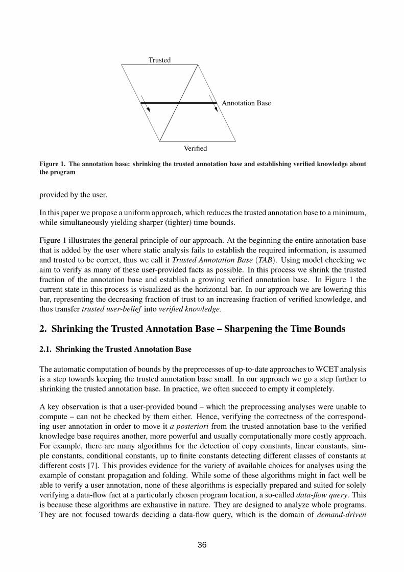
Annotation Base

Verified

Trusted

Figure 1. The annotation base: shrinking the trusted annotation base and establishing verified knowledge aboutthe program

provided by the user.

In this paper we propose a uniform approach, which reduces the trusted annotation base to a minimum,while simultaneously yielding sharper (tighter) time bounds.

Figure 1 illustrates the general principle of our approach. At the beginning the entire annotation basethat is added by the user where static analysis fails to establish the required information, is assumedand trusted to be correct, thus we call it Trusted Annotation Base (TAB). Using model checking weaim to verify as many of these user-provided facts as possible. In this process we shrink the trustedfraction of the annotation base and establish a growing verified annotation base. In Figure 1 thecurrent state in this process is visualized as the horizontal bar. In our approach we are lowering thisbar, representing the decreasing fraction of trust to an increasing fraction of verified knowledge, andthus transfer trusted user-belief into verified knowledge.

2. Shrinking the Trusted Annotation Base – Sharpening the Time Bounds

2.1. Shrinking the Trusted Annotation Base

The automatic computation of bounds by the preprocesses of up-to-date approaches to WCET analysisis a step towards keeping the trusted annotation base small. In our approach we go a step further toshrinking the trusted annotation base. In practice, we often succeed to empty it completely.

A key observation is that a user-provided bound – which the preprocessing analyses were unable tocompute – can not be checked by them either. Hence, verifying the correctness of the correspond-ing user annotation in order to move it a posteriori from the trusted annotation base to the verifiedknowledge base requires another, more powerful and usually computationally more costly approach.For example, there are many algorithms for the detection of copy constants, linear constants, sim-ple constants, conditional constants, up to finite constants detecting different classes of constants atdifferent costs [7]. This provides evidence for the variety of available choices for analyses using theexample of constant propagation and folding. While some of these algorithms might in fact well beable to verify a user annotation, none of these algorithms is especially prepared and suited for solelyverifying a data-flow fact at a particularly chosen program location, a so-called data-flow query. Thisis because these algorithms are exhaustive in nature. They are designed to analyze whole programs.They are not focused towards deciding a data-flow query, which is the domain of demand-driven

36

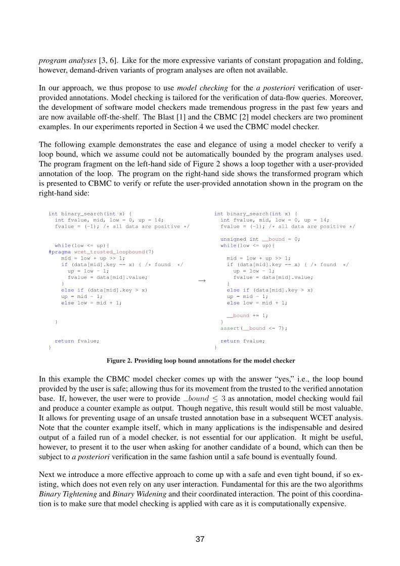
program analyses [3, 6]. Like for the more expressive variants of constant propagation and folding,however, demand-driven variants of program analyses are often not available.

In our approach, we thus propose to use model checking for the a posteriori verification of user-provided annotations. Model checking is tailored for the verification of data-flow queries. Moreover,the development of software model checkers made tremendous progress in the past few years andare now available off-the-shelf. The Blast [1] and the CBMC [2] model checkers are two prominentexamples. In our experiments reported in Section 4 we used the CBMC model checker.

The following example demonstrates the ease and elegance of using a model checker to verify aloop bound, which we assume could not be automatically bounded by the program analyses used.The program fragment on the left-hand side of Figure 2 shows a loop together with a user-providedannotation of the loop. The program on the right-hand side shows the transformed program whichis presented to CBMC to verify or refute the user-provided annotation shown in the program on theright-hand side:

int binary_search(int x) {int fvalue, mid, low = 0, up = 14;fvalue = (-1); /* all data are positive */

while(low <= up){#pragma wcet_trusted_loopbound(7)

mid = low + up >> 1;if (data[mid].key == x) { /* found */up = low - 1;fvalue = data[mid].value;

}else if (data[mid].key > x)up = mid - 1;else low = mid + 1;

}

return fvalue;}

→

int binary_search(int x) {int fvalue, mid, low = 0, up = 14;fvalue = (-1); /* all data are positive */

unsigned int __bound = 0;while(low <= up){

mid = low + up >> 1;if (data[mid].key == x) { /* found */

up = low - 1;fvalue = data[mid].value;

}else if (data[mid].key > x)up = mid - 1;else low = mid + 1;

__bound += 1;}assert(__bound <= 7);

return fvalue;}

Figure 2. Providing loop bound annotations for the model checker

In this example the CBMC model checker comes up with the answer “yes,” i.e., the loop boundprovided by the user is safe; allowing thus for its movement from the trusted to the verified annotationbase. If, however, the user were to provide bound ≤ 3 as annotation, model checking would failand produce a counter example as output. Though negative, this result would still be most valuable.It allows for preventing usage of an unsafe trusted annotation base in a subsequent WCET analysis.Note that the counter example itself, which in many applications is the indispensable and desiredoutput of a failed run of a model checker, is not essential for our application. It might be useful,however, to present it to the user when asking for another candidate of a bound, which can then besubject to a posteriori verification in the same fashion until a safe bound is eventually found.

Next we introduce a more effective approach to come up with a safe and even tight bound, if so ex-isting, which does not even rely on any user interaction. Fundamental for this are the two algorithmsBinary Tightening and Binary Widening and their coordinated interaction. The point of this coordina-tion is to make sure that model checking is applied with care as it is computationally expensive.

37

2.2. Sharpening the Time Bounds

2.2.1. Binary Tightening

Suppose a loop bound has been proven safe, e.g. by verifying a user-provided bound by model check-ing or by a program analysis. Typically, this bound will not be tight. In particular, this will hold foruser-provided bounds. In order to exclude channeling an unsafe bound into the trusted annotationbase, the user will generously err on the side of caution when providing a bound. This suggests thefollowing iterative approach to tighten the bound, which is an application of the classical pattern of abinary search algorithm, thus called binary tightening in our scenario.

Let b0 denote the value of the initial bound, which is assumed to be safe. Per definition b0 is apositive integer. Then: call procedure binaryT ightening with the interval [0..b0] as argument, wherebinaryT ightening([low..high]) is defined as follows:

1. Let m = d low+high2

e.2. ModelCheck(m is a safe bound):

3. yes: low = m: return mlow = m− 1: ModelCheck(low is a safe bound)

yes: return low no: return motherwise: binaryT ightening([low..m])

4. no: high = m: return falsehigh = m + 1: ModelCheck(high is a safe bound)

yes: return high no: return falseotherwise: binaryT ightening([m..high])

Obviously, binaryT ightening terminates. If it returns false, a safe bound tighter than that of theinitial bound b0 could not be established. Otherwise, i.e., if it returns value b, this value is the leastsafe bound. This means b is tight. If it is smaller than b0, we succeeded to sharpen the bound.

Binary widening described next allows for proceeding in the case where a safe bound is not known apriori. If a safe bound (of reasonable size) exists, binary widening will find one, without any furtheruser interaction.

2.2.2. Binary Widening

Binary widening is dual to binary tightening. Its functioning is inspired by the risk-aware gamblerplaying roulette, who exclusively bets on 50% chances like red and black. Following this strategy, inprinciple, any loss can be flattened by doubling the bet the next game. In reality, the maximum betallowed by the casino or the limited monetary resources of the gambler, whatever is lower, prevent thisstrategy to work out in reality. Nonetheless, the idea of an externally given limit yields the inspirationfor the Binary Widening algorithm to avoid looping if no safe bound exists. A simple approach is tolimit the number of recursive calls of binary widening to a predefined maximum number. The versionof binary widening we present below uses a different approach. It comes up with a safe bound, if one

38

exists, and terminates, if the size of the bound is too big to be reasonable, or does not exist at all. Thisdirectly corresponds to the limit set by a casino to a maximum bet.

Let b0 be an arbitrary number, b0 ≥ 1, and let max be the maximum value for a safe bound con-sidered reasonable. Then: Call procedure binaryWidening with b0 and max as arguments, wherebinaryWidening(b, limit) is defined as follows:

1. if b > limit: return false

2. ModelCheck(b is a safe bound):

3. yes: return b

4. no: binaryWidening(2 ∗ b, limit)

Obviously, binaryWidening terminates.1 If it returns false, at most a bound of a size consideredunreasonably big exists, if at all. Otherwise, i.e., if it returns value b, this value is a safe bound. Theratio behind this approach is the following: if a safe bound exists, but exceeds a predefined threshold,it can be considered practically useless. In fact, this scenario might indicate a programming error andshould thus be reported to the programmer for inspection. A more refined approach might set thisthreshold more sophisticatedly, by using application dependent information, e.g., such as a coarseestimate of the execution time of a single execution of the loop and a limit on the overall executiontime this loop shall be allowed for.

2.2.3. Coordinating Binary Tightening and Widening

Once a safe bound has been determined using binary widening, binary tightening can be used tocompute the uniquely determined safe tight bound. Because of the exponential resp. logarithmicbehaviour in the selection of arguments for binary widening and tightening, model checking is calledmoderately often. This is the key for the practicality of our approach, which we implemented inour WCET analyzer TuBound, as described in Section 3. The results of practical experiments weconducted with the prototype implementation are promising. They are reported in Section 4.

3. Implementation within TuBound

3.1. TuBound

TuBound [9] is a research WCET analyzer tool working on a subset of the C++ language. It isunique for uniformly combining static program analysis, optimizing compilation and WCET calcula-tion. Static analysis and program optimization are performed on the abstract syntax tree of the inputprogram. TuBound is built upon the SATIrE program analysis framework [12] and the TERMITEprogram transformation environment.2 TuBound features an array of algorithms for loop analysis ofdifferent accuracy and computation cost including sophisticated analysis methods for nested loops. Adetailed account of these methods can be found in [8].

1In practice, the model checker might run out of memory before verifying a bound, if it is too large, or may take too muchtime for completing the check.

2http://www.complang.tuwien.ac.at/adrian/termite

39

assertions(..., Statement, AssertedStatement) :-Statement = while_stmt(Test, basic_block(Stmts, ...), ...),get_annot(Stmts, wcet_trusted_loopbound(N), _),

counter_decl(’__bound’, ..., CounterDecl),counter_inc(’__bound’, ..., Count),counter_assert(’__bound’, N, ..., CounterAssert),

AssertedStatement =basic_block([CounterDecl,

while_stmt(Test, basic_block([Count|Stmts], ...), ...),CounterAssert], ...).

Figure 3. Excerpt from the source-to-source transformer T

3.2. Implementation

The Binary Widening/Tightening algorithms are implemented by means of a dedicated TERMITEsource-to-source transformer T . For simplicity and uniformity we assume that all loops are struc-tured. In our implementation unstructured goto-loops are thus transformed by another source-to-source transformer T ′ into while-loops beforehand, where possible. On while-loops the transformerT works by locating the first occurrence of a wcet trusted loopbound(N) annotation in the pro-gram source and then proceeding to rewrite the encompassing loop as illustrated in the example ofFigure 3.3 Surrounding the loop statement, a new compound statement is generated, which accom-modates the declaration of a new unsigned counter variable which is initialized to zero upon enteringthe loop. Inside the loop, an increment statement of the counter is inserted at the very first location.After the loop, an assertion is generated which states that the count is at most of value N , where thisvalue is taken from the annotation (cf. Figure 2).

The application of the transformer is controlled by a driver, which calls the transformer for everytrusted annotation contained in the source code. Depending on the result of the model checker andthe coordinated application of the algorithms for binary widening and tightening, the value and thestatus of each annotation is updated. In the positive case, this means the status is changed from trustedannotation to verified knowledge, and the value of the originally trusted bound is replaced by a sharper,now verified bound. Figure 4 shows a snapshot of processing the janne complex benchmark. In thisfigure, the status and value changes are highlighted by different colors.

4. Experimental Results

We implemented our approach as an extension of the TuBound WCET analyzer and applied the ex-tended version to the well-known Malardalen WCET benchmark suite. As a baseline for comparisonwe used the 2008 version of TuBound, which took part in the 2008 WCET Tool Challenge [5], lateron called the basic version of TuBound. In the spirit of the WCET Tool Challenge [4, 5] we doencourage authors of other WCET analyzers to carry out similar experiments.

Our experiments conducted were guided by two questions: “Can the number of automatically boundedloops be significantly increased?” and “How expensive is the process?”. The benchmarks were per-formed on a 3 GHz Intel Xeon processor running 64-bit Linux. The model checker used was CBMC

3For better readability, the extra arguments containing file location and other bookkeeping information are replaced by“...”.

40

...int complex(int a, int b){while(a < 30) {

#pragma wcet_trusted_loopbound(30)while(b < a) {

#pragma wcet_trusted_loopbound(30)if (b > 5)b = b * 3;

elseb = b + 2;

if (b >= 10 && b <= 12)a = a + 10;

elsea = a + 1;

}a = a + 2;b = b - 10;

}return 1;

}...

→

...int complex(int a, int b){

while(a < 30) {#pragma wcet_loopbound(16)

{unsigned int __bound = 0U;while(b < a){

#pragma wcet_trusted_loopbound(30)++__bound;

if (b > 5)b = b * 3;

elseb = b + 2;

if (b >= 10 && b <= 12)a = a + 10;

elsea = a + 1;

}assert(__bound <= 30U);

}a = a + 2;b = b - 10;

}return 1;

}...

Containing two trusted loop annotations Outer loop annotation verified and tightened, inner being checked

Figure 4. Illustrating trusted bound verification and tightening

2.9, which we applied to testing loop bounds up to the size of 213 = 8192 using a timeout of 120seconds and a maximum unroll factor of 213 + 1. The “compress” and “whet” benchmarks containedunstructured goto-loops; as indicated in Section 3.2 these were automatically converted into do-whileloops beforehand by a source-to-source transformation.

Our findings are summarized in Table 1. Column three of this table shows the percentage of loops thatcan be bounded by the basic version of TuBound; column four shows the total percentage of loops theextended version of TuBound was able to bound. The last column shows the accumulated runtime ofthe model checker for the remaining loops.

Comparing columns three and four reveals the superiority of the extended version of TuBound overits basic variant. The extended version succeeds to bound 67% of the loops the basic version couldnot bound.

Considering column five, it can be seen that the model checker terminates quickly on small prob-lems but that the runtime and space requirements can increase to practically infeasible amounts onproblems suffering from the state explosion problem. Such a behaviour can be triggered, if the initial-ization values which are part of the majority of the Malardalen benchmarks are manually invalidatedby introducing a faux dependency on e.g. argc. This demonstrates that model checking is to beused with care or the model checker be fed with additional information guiding and simplifying theverification task.

The fully-fledged variant of our approach, which we highlight in the next section is tailored towardsthis goal.

41

Benchmark Loops TuBound basic with Model Checking Runtimebs 1 0.0% 100.0% 0.03sduff 2 50.0% 50.0% 0sfft1 11 54.5% 81.8% 0.43sjanne complex 2 0.0% 100.0% 0.18sminver 17 94.1% 100.0% 0.06snsichneu 1 0.0% 100.0% 5.59sqsort-exam 6 0.0% 66.6% 0.02sstatemate 1 0.0% 100.0% 0.06swhet 11 90.9% 90.9% 0sadpcm 18 83.3% 83.3% timeoutcompress 8 25.0% 25.0% timeoutfir 2 50.0% 50.0% timeoutinsertsort 2 0.0% 0.0% timeoutlms 10 60.0% 60.0% timeoutselect 4 0.0% 0.0% timeoutbsort100 3 100.0% 100.0% –cnt 4 100.0% 100.0% –cover 3 100.0% 100.0% –crc 3 100.0% 100.0% –edn 12 100.0% 100.0% –expint 3 100.0% 100.0% –fdct 2 100.0% 100.0% –fibcall 1 100.0% 100.0% –jfdctint 3 100.0% 100.0% –lcdnum 1 100.0% 100.0% –ludcmp 11 100.0% 100.0% –matmult 5 100.0% 100.0% –ndes 12 100.0% 100.0% –ns 4 100.0% 100.0% –qurt 1 100.0% 100.0% –sqrt 1 100.0% 100.0% –st 5 100.0% 100.0% –recursion 0 – – –Total Percentage 77.0% 84.7%

Table 1. Results for the Malardalen benchmarks

42

. . .

Model Checking

Constant Propagation

Interval Analysis

Constraint Propagation

Profiling

Figure 5. Pool of complementary analysis techniques with different complexity

5. Extensions: The Fully Fledged Approach

The shrinking of the trusted annotation base and sharpening of time bounds, as described in Section 2,is based on model checking. Based on our experience, we believe that the model checking approachcan be very valuable in the real world when (i) it is combined with advanced program slicing tech-niques to reduce the state space and (ii) the results of static analyses (like TuBound’s variable-intervalanalysis) are used to narrow the value ranges of variables, thus regaining a feasible problem size. Thisleads to the following extension of our approach to improve efficiency:

1. By using a pool of analysis techniques with different computational complexity: As shown inFigure 5, model checking is considered as one of the most complex analysis methods. On theother side, techniques like constant propagation or interval analysis are relatively fast. Thuswe are interested in exploiting the fast techniques wherever beneficial and using the relativelycomplex techniques rarely.

2. By using a smart activation mechanism for the different analysis techniques: As shown on theright of Figure 5 we are interested in the interaction of the different analysis techniques. Wedo not aim to use the pool of analysis techniques in waves of different complexity, i.e., firstapplying the fast techniques and then gradually shifting towards the more complex techniques.Instead we aim for a smart interaction of the different analysis techniques. For example, when-ever a technique with relatively high computational complexity has been applied, we can againapply techniques of relatively simple complexity to compute the closure of flow informationbased on previously obtained results; thus squeezing the annotation base.

We also think that profiling techniques are useful to guide the heuristics to be used within our staticanalysis techniques. For example, execution samples obtained by profiling can be used to elicit propo-sitions to be verified by model checking.

The fully fledged approach envisioned in this section provides the promising potential as a researchplatform for complementing program analysis techniques.

43

6. Conclusions

Model checking has been used before in the context of WCET analyzers. Examples of our own relatedwork are the ForTAS [13], MoDECS [14], and ATDGEN projects [10, 11], which are concerned withmeasurement-based WCET analysis. In these three projects, model checking is used to generate testdata for the execution of specific program paths. Intuitively, in these applications the model checkeris presented with formulae stating that a specific program path is infeasible. If these formulae canbe refuted by the model checker, the counter examples generated provide the test data ensuring theexecution of the particular paths. Otherwise, the paths are known to be infeasible. Hence, the searchfor test data is in vain. In these applications the counter examples generated in the course of failingmodel checker runs are the truly desired output, whereas successful runs are of less interest stoppingjust the search for test data for the path under consideration. This is in contrast and opposite toour application of shrinking the trusted annotation base. In our application, the counter example ofa failed model checker run is of little interest. We are interested in successful runs of the modelchecker as they allow us to change a trusted annotation into verified knowledge. This opens a newapplication domain for model checking in the field of WCET analysis. Our preliminary practicalresults demonstrate the practicality and power of this approach.

References

[1] BEYER, D., HENZINGER, T., JHALA, R., AND MAJUMDAR, R. The software modelchecker Blast. International Journal on Software Tools for Technology Transfer (STTT) 9, 5-6 (October 2007), 505–525.

[2] CLARKE, E., KROENING, D., AND LERDA, F. A tool for checking ANSI-C programs.In Tools and Algorithms for the Construction and Analysis of Systems (TACAS 2004) (2004),K. Jensen and A. Podelski, Eds., vol. 2988 of Lecture Notes in Computer Science, Springer,pp. 168–176.

[3] DUESTERWALD, E., GUPTA, R., AND SOFFA, M. L. A practical framework for demand-driven interprocedural data flow analysis. ACM Transactions on Programming Languages andSystems 19, 6 (1997), 992 – 1030.

[4] GUSTAFSSON, J. The WCET tool challenge 2006. In Preliminary Proc. 2nd InternationalIEEE Symposium on Leveraging Applications of Formal Methods, Verification and Validation(Paphos, Cyprus, November 2006), pp. 248 – 249.

[5] HOLSTI, N., GUSTAFSSON, J., (EDS.), G. B., BALLABRIGA, C., BONENFANT, A.,BOURGADE, R., CASSE, H., CORDES, D., KADLEC, A., KIRNER, R., KNOOP, J., LOKU-CIEJEWSKI, P., MERRIAM, N., DE MICHIEL, M., PRANTL, A., RIEDER, B., ROCHANGE,C., SAINRAT, P., AND SCHORDAN, M. WCET Tool Challenge 2008: Report. In Proc.8th International Workshop on Worst-Case Execution Time Analysis (WCET 2008) (Prague,Czech Republic, July 2008), Osterreichische Computer Gesellschaft, pp. 149–171. ISBN: 978-3-85403-237-3.

[6] HORWITZ, S., REPS, T., AND SAGIV, M. Demand interprocedural dataflow analysis. In Proc.3rd ACM SIGSOFT Symposium on the Foundations of Software Engineering (FSE-3) (1995),pp. 104 – 115.

44

[7] MUCHNICK, S. S. Advanced Compiler Design & Implementation. Morgan Kaufmann Pub-lishers, Inc., 1997. ISBN 1-55860-320-4.

[8] PRANTL, A., KNOOP, J., SCHORDAN, M., AND TRISKA, M. Constraint solving for high-level wcet analysis. In Proc. 18th International Workshop on Logic-based methods in Program-ming Environments (WLPE 2008) (Udine, Italy, December 2008), pp. 77–89.

[9] PRANTL, A., SCHORDAN, M., AND KNOOP, J. TuBound – a conceptually new tool forworst-case execution time analysis. In Proc. 8th International Workshop on Worst-Case Execu-tion Time Analysis (WCET 2008) (Prague, Czech Republic, July 2008), Osterreichische Com-puter Gesellschaft, pp. 141–148. ISBN: 978-3-85403-237-3.

[10] RIEDER, B. Measurement-Based Timing Analysis of Applications written in ANSI-C. PhDthesis, Technische Universitat Wien, Vienna, Austria, 2009 (forthcoming).

[11] RIEDER, B., WENZEL, I., AND PUSCHNER, P. Using model checking to derive loop boundsof general loops within ANSI-C applications for measurement-based WCET analysis. In Proc.6th International Workshop on Intelligent Solutions in Embedded Systems (WISES 2008) (Re-gensburg, Germany, July 2008).

[12] SCHORDAN, M. Source-To-Source Analysis with SATIrE – an Example Revisited. In Proceed-ings of Dagstuhl Seminar 08161: Scalable Program Analysis (April 2008), Germany, Dagstuhl.

[13] VIENNA UNIVERSITY OF TECHNOLOGY AND TU DARMSTADT. The ForTAS project.Web page (http://www.fortastic.net). Accessed in June 2009.

[14] WENZEL, I., KIRNER, R., RIEDER, B., AND PUSCHNER, P. Measurement-based timinganalysis. In Proc. 3rd International Symposium on Leveraging Applications of Formal Methods,Verification and Validation (Porto Sani, Greece, October 2008).

45

WCET ANALYSIS OF MULTI-LEVELSET-ASSOCIATIVE DATA CACHES

Benjamin Lesage , Damien Hardy and Isabelle Puaut1

AbstractNowadays, the presence of cache hierarchies tends to be a common trend in processor architectures,even in hardware for real-time embedded systems. Caches areused to fill the gap between the proces-sor and the main memory, reducing access times based on spatial and temporal locality properties oftasks. Cache hierarchies are going even further however at the price of increased complexity. In thispaper, we present a safe static data cache analysis method for hierarchies of non-inclusive caches.Using this method, we show that considering the cache hierarchy in the context of data caches allowstighter estimates of the worst case execution time than whenconsidering only the first cache level. Wealso present considerations about the update policy for data caches.

1. Introduction

It is crucial in hard real-time systems to prove that tasks meet their deadlines in all situations, includingthe worst-case. This proof needs an estimation of the worst-case execution time (WCET) of every tasktaken in isolation. WCET estimates have to be safe, i.e. larger than or equal to any possible executiontime. Moreover, they have to be tight, i.e. as close as possible to the actual WCET. Thereof, WCETestimation techniques have to account for all possible execution paths in the program and determinethe longest one (high-levelanalysis). They also have to account for the hardware the task is runningon (low-levelanalysis).

Cache memories are introduced to decrease the access time tothe information due to the increasinggap between fast micro-processors and relatively slower main memories. Architectures with cachesare now commonly used in embedded real-time systems due to the increasing demand for computingpower of many embedded applications. The presence of cachesin real-time systems makes WCETestimation difficult due to the dynamic behaviour of caches.Safely estimating WCET on architectureswith caches requires a knowledge of all possible cache contents at every program point, and requiressome knowledge of the cache replacement policy and, in case of data caches, update policy.

During the last decade, much research has been undertaken topredict WCET in architectures equippedwith caches. Regarding instruction caches, static cache analysis methods [13, 14, 18, 3] have beendesigned and recently, extended to hierarchies of non-inclusive caches [7]. To overcome predictabilityissues, as the ones due to the replacement policies, is the family of approaches like locking [15, 20].The latter methods family suits well to data caches [19, 11],whose analysis suffers from imprecisestatic accessed data address prediction. Indeed, if precise address prediction in the context of in-struction caches has been mastered, for data caches, it remains an important concern. Nonetheless,existing methods for instruction caches have also been modified [16, 17, 4] to tackle with accesseswhose target can only be over-approximated using a range of addresses.

To the best of our knowledge, no safe static cache analysis method has been proposed so far to predictworst-case data cache behaviour in the presence of a data cacheshierarchy. The issues to be tackledwhen designing such an analysis are twofold. On the one hand,the prediction of cache levels impacted

1IRISA, University of Rennes 1, Rennes, France

46

by a memory reference is required to estimate the induced caches accesses. On the other hand, writesto the caches have to be considered, because they may introduce additional cache accesses. Ensuedpredictability problems may even get exacerbated by the lack of precise knowledge about accessedaddresses.

The contribution of this paper is the proposal of a new safe static cache analysis method for multi-levelnon-inclusive set-associative data caches. All levels of cache are analysed sequentially. Similarly toour previous work for instruction caches [7], the safety of the proposed method relies on the intro-duced concept of acache access classification, defining which references may occur at every cachelevel and have to be considered by the cache analysis of that level, in conjunction with the more tra-ditional cache hit/miss classification. This paper presents experimental results showing that in mostcases WCET estimates are tighter when considering the cachehierarchy than when considering theL1 cache only.

The rest of the paper is organized as follows. Related work issurveyed in Section 2. Section 3 presentsthe type of caches to which our analysis applies. Section 4 then details our proposal. Experimentalresults are given in Section 5. Finally, Section 6 concludeswith a summary of the contributions ofthis paper, and gives directions for future work.

2. Related work

Caches in real-time systems raise timing predictability issues due to their dynamic behaviour andtheir replacement policy. Many static analysis methods have been proposed in order to produce a safeWCET estimate on architectures with caches. To be safe, existing cache analysis methods determineeverypossible cache contents at every point in the execution, considering all execution paths alto-gether. Possible cache contents can be represented as sets of concrete cache states[9] or by a morecompact representation calledabstract cache states(ACS) [18, 3, 14, 13].

Two main classes of approaches [18, 13] exist for the static WCET analysis on architectures witha single level of instruction cache. In [18] the approach is based onabstract interpretation[2] anduses ACSs. In this approach, three different analyses are applied which use fixpoint computationto determine if a memory block isalwayspresent in the cache (Must analysis), if a memory blockmaybe present in the cache (May analysis), or if a memory block will not be evicted after it hasbeen first loaded (Persistenceanalysis). Acache hit/miss classification(e.g. always hit, first miss...)can then be assigned to every instruction based on the resultof the three analyses. This approachoriginally designed for set-associative instruction caches implementing theleast recently used(LRU)replacement policy has been extended for different cache replacement policies in [8] for instructioncaches. In [13],static cache simulationis used to determine every possible content of the instructioncache before each instruction. Static cache simulation computes abstract cache states using data-flowanalysis. Acache hit/miss classificationis used to classify the worst-case behaviour of the cache foragiven instruction. The base approach, initially designed for direct-mapped caches, was later extendedto set-associative instruction caches in [14].

A peculiarity of data caches, compared to instruction caches, arises as the precise target of somereferences may not be statically computable. A first solution is to consider these imprecise accessesas in [17] and [4], improvements to [18]. Therefore, we base our cache analysis on these studies.

An alternative solution to deal with data caches areCache Miss Equations(CME) [19, 11, 21]. Toestimate cache behaviour, the iteration space of loop nestsis represented as a polyhedron.Reusevectors[22] are then defined between points of the iteration space. CME are set up and resolved toaccurately locate misses. This method has been successfully applied to data caches in combination

47

with locking [19]. However, according to the authors, this approach suffers from a lack of support fordata dependent conditionals.

Another scarcely addressed characteristic of data caches is the impact of memory modifying instruc-tions. In [5], an analysis was proposed based on thewrite-backupdate policy. Modified data in acache are copied back to the main memory upon eviction. The objective is thus to estimate thewritebacks, i.e. the moment when a modified data might be replaced in the cache. In a first step towardsa more generic solution, we chose to use thewrite-throughupdate policy as it removes the need ofwrite backsmonitoring.

Finally, about the hierarchy of data caches, we already explored a solution to this problem in [7] inthe context of instruction caches. Introducing the conceptof cache access classification(CAC), wesafely identify references that may, must or never occur at every level in the cache hierarchy. Thispaper presents to which extent this approach can be applied to data caches.

3. Assumptions and notations

As this study focuses on data caches, code is assumed not to interfere with data in the differentconsidered caches. There is no assumption on the means used to achieve this separation, whether theyare software or hardware based. An architecture without timing anomalies, caused by interactionsbetween caches and pipelines [12], is however assumed.

The considered cache hierarchy is composed ofN levels of data caches. Each cache implementsthe LRU replacement policy. Using this policy, cache blocksin a cache set are logically orderedaccording to their age. If a cache set is full, upon a load in this set, the evicted block is the oldest onewhereas the most recently accessed block is the youngest one.

A datum accessed by an instruction should be located in a single memory block. Cache line size oflevelL is assumed to be a multiple of the cache line size of levelL − 1. However, no assumption ismade concerning the cache sizes or associativities. Furthermore, the following properties are assumedto hold:

P1.[load] A piece of information is searched for in the cache of levelL if, and only if, a cache missoccurred when searching it in the cache of levelL − 1. Cache of level1 is always accessed.

P2.[load] Every time a cache miss occurs at cache levelL, the entire cache line containing the miss-ing piece of information is loaded into the cache of levelL.

P3.[store] The modification issued by a store instruction goes all the way through the memory hierar-chy. Writes to the cache levels where the written memory block is already present are triggered,along with the update of the main memory. Otherwise, if the information is absent from a cache,this cache level is left unchanged.

P4.[store] Upon a write in a cache block, wherever is the cache in the hierarchy, no block age modi-fication is induced2.

P5. There are no action on the cache contents (i.e. lookup/modification) other than the ones men-tioned above.

Property P1 rules out architectures where cache levels are accessed in parallel to speed up informationlookup. P2 excludes architectures with exclusive caches, whereas P5 filters out cache hierarchiesensuring inclusion.

Properties P3 and P4 on the other hand address the store instructions behaviour. P3 ensures the use of

2Note that this is not a strong assumption but its alleviationis left as future work.

48

thewrite-throughupdate policy. In combination with P3, P4 corresponds amongother things to thewrite-no-allocateupdate policy for members of the cache hierarchy, as illustrated in Figure 1.

memoryMain

L1

L2 X := w

age +

w

age +

Occurrences of memory location Xin the memory hierarchy

Store w,Xw

Figure 1: Example of the memory hi-erarchy behaviour upon a store in-struction (write-through and write-no-allocate policies).

Finally, the latencies to access the different levels of themem-ory hierarchy are assumed to be bounded and known.

We define amemory referenceas a reference todata in thememory triggered by a load or store instruction in a fixed callcontext; a memory reference is tied to a unique instruction anda unique call context.

4. Data Cache Analysis

This section introduces most of the involved steps in our com-putation of WCET contribution for hierarchies of data caches.The structure of the whole method is outlined in Figure 2.

CFG Extraction

Address Analysis

Multi−Level Cache Analysis

Task Executable

CFG

Memory references

Cache Hit/Miss ClassificationCache Access Classifications

WCETWorst−case Execution Path

Worst Case Analysis

Figure 2: Complete taskanalysis overview

After a first step that extracts aControl Flow Graphfrom the analysedexecutable, a data address analysis (§ 4.1) is performed. The objectiveis to attach to every memory reference a safe estimate of the accessedaddresses.

Then, the caches of the hierarchy are analysed one after the other (§ 4.2)based on address information. For each cache level and each instruction is-suing memory operations, acache hit/miss classification(CHMC) is com-puted. These classifications represent the worst-case behaviour of thiscache level with regards to this instruction.

To be safe, the analysis of a cache level further relies oncache accessclassifications(CAC, introduced in§ 4.3) which discloses, given a mem-ory reference, a safe approximation of whether or not it occurs at a cachelevel.

In the end, a timing analysis of memory references (§ 4.4), consideringdata caches, is performed with the help of both the CHMC and CAC foreach cache level. Such information may then be used to compute the longest possible execution pathand finally the WCET of the task.

4.1. Address analysis

The address analysis, in the context of data caches, computes for every memory reference, the memorylocation it may access. Such information may however not be precisely computable, hence producingan over-approximation to yield safe values for subsequent analyses. These over-approximations takethe form of ranges of possibly accessed memory blocks instead of a reference to a precise memoryblock.

The address analysis uses data-flow analyses which first computes stack frames addresses for eachvalid call context and then analyse register contents for each basic block. Considering both global andon stack accesses, the precise address of a scalar is yieldedwhereas the whole array address range isreturned for accesses to array elements. Note that the analysis used below is the one proposed in [6].

49

4.2. Single level data cache analysis

Below, a data cache analysis abstracted from the multi-level aspect is introduced. All references areanalysed and access filtering, according to other cache levels, is introduced later (§ 4.3). The analysismethod is presented along with the different mechanisms to handle the specificities of data caches,compared to instruction caches.

Focusing on data caches, the timing analysis of memory references is performed using the worst-casebehaviour of this data cache for each memory reference. Thisknowledge is itself based on the cachecontents at the studied program point, thus requiring a safeestimate of memory blocks present in thecache.

A cache hit/miss classification(CHMC) is used to model the defined cache behaviours with regardsto a given memory reference. To such a reference has already been attached a set of possibly accessedmemory blocks by the address analysis. This set of memory blocks is used to compute the CHMC:

always-hit(AH) : all the possibly accessed memory blocks are guaranteed to be in the cache;first-miss(FM) : for every possibly accessed memory block, once it has been first loaded in the cache,

it is guaranteed to stay in the cache afterwards;always-miss(AM) : all the possibly accessed memory blocks are known to beabsent from the cache;content-independent(CI) : if the behaviour of the memory reference does not depend on the cache

contents. The CI classification is used for store instructions, which, according to our hypotheses(§ 3) does not depend on the cache contents;

not-classified(NC) : if none of the above applies.

Abstract cache states(ACSs) are used to collect information along the task CFG. This abstractionallows the modelling of a combination of concrete cache states, in terms of present memory blocksand their relative age. This is required as all paths have to be considered altogether to yield safevalues. Different analyses, similarly to [18], are defined to collect information about cache contentsat every program point. For each analysis, fixpoint computation is applied on the program CFG, forevery call context:

aMustanalysis determines if a memory block is always present in the cache, at a given point, thusallowing aalways-hitclassification;

aPersistenceanalysis determines if a memory block will not be evicted from the cache once it hasbeen first loaded, as in the definition of thefirst-missclassification;

aMayanalysis determines if a memory block may be in the cache at a given point, otherwise theblock is guaranteed not to be in the cache thus possibly allowing aalways-missclassification.If, at a given point, some possibly accessed memory blocks are present in the May analysis butneither in the Must nor the Persistence one, thenot-classifiedclassification is assumed for thismemory reference.

Then, for each memory reference, its set of possibly accessed memory block is compared to thememory blocks inside the input ACS computed by each analysis.

Join functions : For instructions on branch reconvergence, theJoinMust, JoinPersistence andJoinMay

(respectively for the Must, Persistence and May analysis) are used as a mean to compute input ACS:

JoinMust computes the intersection of memory blocks present in the input ACSs, keeping for eachone its maximal age as shown in Figure 3a;

JoinPersistence keeps the union of memory blocks present in the input ACSs, asfor JoinMust, themaximal age of memory blocks is kept;

50

JoinMay computes the union of memory blocks present in the input ACSs, keeping for each one itsminimal age.

Considering data caches, these functions are the same as theones defined for instruction caches [18].

Update functions : The effects of memory references on the cache are modelled using theUpdateMust,UpdatePersistence andUpdateMay for the Must, Persistence and May analysis respectively. Inall thecases, only load instructions have an impact on the cache contents. Store instructions have no im-pact on ACSs (§ 3, use of the write-through and write-no-allocate update policies). Considering datacaches, theUpdatefunction of the different analyses is of particular interest. Indeed, it has to dealwith accesses indeterminism, when a precise memory location cannot be statically defined for a loadinstruction. Two options have to be considered.

On the one hand, the precise accessed memory block may have been computed by the address anal-ysis. TheUpdatefunction is then pretty straightforward, as illustrated inFigure 3b for the Mustanalysis. Thus considering theUpdateMust, the accessed block is put at the head of its cache set andthe younger lines are shifted, i.e. made older and evicted iftoo old. Note that memory blocks outsidean ACS are supposed to be older than the ones present in this same ACS. Furthermore, the differentUpdatefunctions behaviour in this case is the same than for instructions [18].

On the other hand, when the address analysis yields a set of possibly accessed memory blocks fora memory reference, only one member of this set is actually accessed. To model this behaviour, acopy of the input ACS is created, using the appropriateUpdatefunction, for each possibly accessedmemory block. Then, all the updated copies are unified, this time using the appropriateJoin functionto produce an ACS. This process is illustrated on Figure 3c, for the Must analysis.

{a}{c}

LRU replacementpolicy intersection

+ maximal age{} {a}

+age

{a} {b}abstract cache setof 2−way

(a) Join function of Must analysis

+age

{a} {b} ACS in

LRU replacementpolicy

{a}{c} ACSout

[c]

abstract cache setof 2−way

(b) Update function of Mustanalysis while accessingmemory block c.

+age

{a} {b} ACSin

{a}{c}

{} {a}

LRU replacementpolicy

abstract cache setof 2−way

[a,c]

{b}{a}

[a] [c]

ACSout

(c) Update function while accessinginterval of blocks [a,c]

Figure 3: UpdateMust andJoinMust functionsTermination of the analyses. In the context of abstract interpretation, to prove the termination of ananalysis, it is sufficient to prove the use of a finite abstractdomain and the monotony of the transferfunctions. ACS domain was shown to be finite in [18]. Moreover, [18] demonstrates the monotony oftheJoinx andUpdatex functions (x ∈ {Must, Persistence or May}), for instructions and thus foraccesses to precise memory blocks. In our case, the modification to be proved is the one applied tothis sameUpdatex function to handle accesses to possibly referenced memory blocks.

When an ACS is updated using a set of possibly referenced memory blocks for an analysisx, acomposition of theUpdatex, for each block, and theJoinx function is performed. As the compositionof monotonic functions is monotonic, our modifications ensure monotony. ⊓⊔

4.3. Multi-level analysis

The cache analysis described in§ 4.2 does not support hierarchies of caches, i.e. all referencesare considered for the caches by the analysis. But, a memory reference may not occur in all the

51

cache levels of the hierarchy. This filtering by previous caches in the hierarchy, impacts the cachecontents. Hence, caches are analysed one after the other, from cache level 1 toN , andcache accessclassifications(CACs), as defined in [7], are used to represent occurrences of memory referencer oncache levelL. This is possible as, according to our hypotheses, occurrences of memory referenceson cache levelL (and thusL contents) only depend on occurrences of memory references on cacheslevelsL′ < L.

Cache accessclassification

Level L+1

computationWCET

Cache analysisLevel L

Cache accessclassification

Level LreferencesMemory

Cache hit/missclassification

Level L

Cache analysisLevel L+1

Cache accessclassificationLevel L+2

Cache hit/miss

Level L+1classification

Figure 4: Multi-level non-inclusivedata cache analysis framework

Different classifications have been defined to represent if mem-ory referencer is performed on cache levelL:

Always(A) means that the accessr is always performed atcache levelL,

Never(N) means that the accessr is never performed at cachelevelL,

Uncertain-Never(U-N) indicates that no guarantee can begiven considering the first access to each possibly refer-enced memory block forr, but next accesses are neverperformed at levelL,

Uncertain(U) indicates that no guarantee can be given aboutthe fact that the access tor will or will not be performedat levelL.

For the L1 cache, CAC determination is simple as it was earlierassumed that all memory references will be performed in thiscache level (P1.§ 3). This implies a A classification for everymemory reference, considering the L1 cache.

Concerning greater cache levels, the CAC for memory referencer and cache levelL is defined using both the CAC and the CHMC of the previous levelcache level(see Figure 4) as in [7], to safely model cache filtering in thecache hierarchy. This is illustrated inTable 1.

hh

hh

hh

hh

hh

hh

CACr,L−1

CHMCr,L−1 AH FM AM NC

A N U-N A UN N N N N

U-N N U-N U-N U-NU N U-N U U

Table 1: Cache access classification forlevel L (CACr,L)

Once these classifications have been settled, they have tobe considered in the multi-level cache analysis. The mod-ifications to handle hierarchies of data caches are similarto the modifications to handle hierarchies of instructioncaches [7]. A (respectively N) classification for a giveninstruction, means that the reference is (respectively not)performed on the considered cache level which should bemodelled by the analysis. As for the U and U-N classifica-tions, both the cases are possible: the access is performed (A) or not (N) on this cache level. Similarlyto non deterministic accesses, the two alternatives are considered and their outcomes unified usingthe appropriateJoin function of the analysis.

TheUpdatex function,x ∈ {Must, Persistence or May}, is modified to consider these classifica-tions :

Updatemlx (ACSin, r, L) =

Updatex(ACSin, r, L) if CACr,L = AACSin if CACr,L = NJoinx(ACSin, Updatex(ACSin, r, L)) if CACr,L = U ∨ CACr,L = U-N

whereUpdatemlx represents the multi-level version of theUpdatex functions presented earlier (§ 4.2).

This definition can be inflected toUpdatemlMust, Updateml

Persistence or UpdatemlMay using the correspond-

ing UpdateandJoin functions of the Must, Persistence or May analysis respectively.

52

Termination of the analyses. The differences between the multi-level data cache analysis and thesingle-level data cache analysis are theUpdatex functions,x ∈ {Must, Persistence or May}, forthe different analyses. However these functions were proved to be monotonic in section 4.2. Theproof in [7] thus holds for data caches as well. We need to demonstrate that theUpdateml

x function ismonotonic for the four possible values ofCAC.

For an A access,Updatex andUpdatemlx behave identically.Updatex being monotonic,Updateml

x

is also monotonic. Considering a N access,Updatemlx is the identity function and so is monotonic.

Finally, considering an U or U-N access,Updatemlx composesUpdatex andJoinx. These two functions

are monotonic, so is their composition. ThusUpdatemlx is monotonic which guarantees the termination

of our analysis. ⊓⊔

4.4. WCET computation

CHMCs represent the worst-case behaviour of the cache givena memory reference. They are usefulto compute the contribution of references to the WCET. This contribution can then be used in existingmethods to compute the WCET. In our case, we focus on IPET based methods which estimates theWCET by solving anInteger Linear Programming(ILP) problem [10].

The timing of the memory referencer, with regards to the data caches, is divided in two parts.firstandnext respectively distinguish the first and successive iterations of loops. We defineCOST first(r)and COST next(r) as the respective contribution to the WCET of memory reference r for thefirst and successive iterations of the loop in which the reference is enclosed, if any3. If no loopenclosesr, COST first(r) will be implicitly preferred, by the ILP solver, overCOST next(r)as the cost ofr. IndeedCOST first(r) accounts for all first misses of memory referencer andCOST first(r) ≥ COST next(r).

With freqr a variable computed in the context of IPET analysis and representing the execution fre-quency ofr along the worst-case execution path of the task, the following constraints are defined:freqr = freqfirst,r + freqnext,r andfreqfirst,r ≤ 1. The WCET contribution of the referencer withregards to data caches is then defined as:

WCET data contribution(r) = COST first(r) × freqfirst,r + COST next(r) × freqnext,r

As we focus on an architecture without timing anomalies, it is safe to consider that NC referencesbehave like AM ones, which are the worst-case on our architecture. Therefore, U accesses to acache level behave as A ones, from the timing analysis considering data caches point of view4. Wedefinealways contribute(r) andnever contribute(r) as the sets of memory hierarchy levels whichrespectively always or never contribute to the execution latency of memory referencer, with M =N + 1 the main memory in the memory hierarchy:

never contribute(r) = {L | 1 ≤ L ≤ M ∧ CACr,L = N}

always contribute(r) = {L | 1 ≤ L ≤ M ∧ (CACr,L = A ∨ CACr,L = U)}

One option to deal with a FM classification for referencer on cache levelL would be to con-sider, for every execution ofr, that cache levelL + 1 is accessed:CACr,L = U-N ⇒ L ∈always contribute(r). However, it might be overly pessimistic with regards to thesemantic ofthe FM and the de facto inherited U-N classifications. We needadditional notations to depict thisbehaviour and tightenr contribution to the WCET.

Given a memory referencer and a cache levelL, let memory blocksr,L be the set ofr target mem-ory blocks on cache levelL, as computed by the address analysis. This information is computed

3Remember thatr is contextual and attached to a unique instruction. A memoryreference tied to the same instruction, butanother context may be enclosed in different loops.

4From the ACS computing point of view, they keep different meanings.

53

using the cache blocks size of cache levelL. We only need to know a bound on the size of thisset:|memory blocksr,L| = ⌈ Addr ranger

cache block sizeL⌉ with Addr ranger the size of the address range com-

puted by the address analysis for memory referencer andcache block sizeL the size of levelL cacheblocks.

Furthermore, we definemax freqr as the maximum statically computable execution frequency ofreferencer. Such an information is computed as the product of the maximum number of iterations ofall loops containingr: max freqr =

∏

lo∈Loops(r) max iterlo, whereLoops(r) are the loop contain-ing the memory referencer andmax iterlo, the maximum iteration attribute for looplo. Note that thewhole task is itself considered to be a loop enclosing all memory references and whosemax iter = 1,ensuring that themax freq attribute of an otherwise not enclosed in a loop memory reference is1.

Each element ofmemory blockr,L produces at most one miss in the cache levelL, the first time itis accessed, according to the definition of the FM classification. Thus, referencer will not producemore thanmin(max freqr, |memory blocksr,L|) misses on cache levelL.

Note thatmin(freqr, |memory blocksr,L|), with freqr the execution frequency ofr on the worst-case execution path of the task, would be a tighter bound. However, this bound is required to computefreqr and vice versa thus leading to a chicken-and-egg problem.

Once these elements have been defined, we can bound the numberof occurrences of memory refer-encer on cache levelL:

max occurrence(r,L) =

8

>

>

>

>

>

>

<

>

>

>

>

>

>

:

0 if L ∈ never contribute(r)

max freqr if L ∈ always contribute(r)

min(|memory blocksr,L−1|, max occurrence(r,L − 1)) if CHMCr,L−1 = FM

max occurrence(r,L − 1) otherwise

Intuitively, if cache levelL is never (respectively always) accessed by memory reference r, therecannot be any (respectively more thanmax freqr) occurrences ofr on cache levelL. Similarly, therecannot be more occurrences ofr on cache levelL than on cache levelL−1. Finally, if CHMCr,L−1 =FM , only the first accesses to memory blocks belonging tomemory blocksr,L−1 will occur on cachelevelL.

The definition ofCOST next(r) is pretty straightforward, as we only have to count the access latencyof cache levelsL which are guaranteed to always contribute to the timing ofr. Other accesses areconsidered inCOST first(r):

COST next(r) =

8

>

>

>

>

<

>

>

>

>

:

P

L∈ always contribute(r)

ACCESS latencyL if r is a load of data

STORE latency if r is a store of data

0 otherwise

COST first(r) is a bit harder to define. In some cases, we have a bound on the number of occur-rences of a memory referencer on cacheL. As previously stated, the solution of not consideringthese bounds might be unnecessary pessimistic. Therefore,we chose to use theCOST first(r) tohold these additional latencies. It could be understood as considering all the possible first misses inthe first execution ofr, in addition to all the always accessed cache levels latencies:

COST first(r) =

8

>

>

>

>

<

>

>

>

>

:

P

L∈ always contribute(r)

ACCESS latencyL +P

CACr,L=U-NACCESS latencyL × max occurrence(r,L) if r loads data

STORE latency if r stores data

0 otherwise

54

5. Experimental results

5.1. Experimental setup

Cache analysis and WCET estimation. The experiments were conducted on MIPS R2000/R3000binary code compiled with gcc 4.1 with no optimization and with the default linker memory layout.The WCETs of tasks are computed by the Heptane timing analyser [1], more precisely its ImplicitPath Enumeration Technique (IPET). The timing of memory references with regards to data caches isevaluated using the method introduced in Section 4.4. The analysis is context sensitive (functions areanalysed in each different calling context). To separate the effects of caches from those of the otherparts of the processor micro-architecture, WCET estimation only takes into account the contributionof caches to the WCET. The effects of other architectural features are not considered. In particular,timing anomalies caused by interactions between caches andpipelines, as defined in [12] are disre-garded. The cache classificationnot-classifiedis thus assumed to have the same worst-case behaviourasalways-missduring the WCET computation in our experiments. The cache analysis starts with anempty cache state.

Name Description Code size Data size Bss size Stack size(bytes) (bytes) (bytes) (bytes)

crc Cyclic redundancy check computation 1432 272 770 72fft Fast Fourier Transform 3536 112 128 288insertsort Insertsort of an array of 11 integers 472 0 44 16jfdctint Fast Discrete Cosine Transform 3040 0 512 104ludcmp Simultaneous Linear Equations by LU De-

composition2868 16 20800 920

matmult Product of two 20x20 integer matrixes 1048 0 4804 96minver Inversion of floating point 3x3 matrix 4408 152 520 128ns Search in a multi-dimensional array 600 5000 0 48qurt Root computation of quadratic equations 1928 72 60 152sqrt Square root function implemented by Taylor

series544 24 0 88

statemate Automatically generated code by STARC(STAtechart Real-time-Code generator)

8900 32 290 88

Table 2: Benchmark characteristics

Benchmarks. The experiments were conducted on a subset of the benchmarksmaintained by MalardalenWCET research group5. Table 2 summarizes the characteristics characteristics (size in bytes of sec-tionstext, data, bss(unitialized data) andstack).

Cache hierarchy. The results are obtained on a 2-level cache hierarchy composed of a 4-way L1 datacache of 1KB with a cache block size of 32B and a 8-way L2 data cache of 4KB with a cache blocksize of 32B. A perfect private instruction cache, with an access latency of one cycle, is assumed. Allcaches are implementing a LRU replacement policy. Latencies of 1 cycle (respectively 10 and 100cycles) are assumed for the L1 cache (respectively the L2 cache and the main memory). Upon storeinstructions a latency of 150 cycles is assumed to update thewhole memory hierarchy.

5.2. Considering the cache hierarchy

To evaluate the interest of considering the whole cache hierarchy, two configurations are compared inTable 3. In the first configuration, only the L1 cache is considered and all accesses to the L2 cacheare defined as misses (WCETL1, column 1). In the other configuration (WCETL1&L2, column 2),both the L1 and the L2 caches are analysed using our multi-level static cache analysis (§ 4.3). Table 3presents these results for the two cases using the tasks WCETas computed by our tool and based onour multi-level static analysis. The presented WCET are expressed in cycles.

5http://www.mrtc.mdh.se/projects/wcet/benchmarks.html

55

The third column of Table 3 represents the improvement, for each analysed task, attributable to theconsideration of the second cache level of the hierarchy:WCETL1−WCETL1&L2

WCETL1.

Benchmark WCET consid-ering only a L1cache

WCET consid-ering both L1and L2 cache

Improvementconsidering theL2 cache

(cycles) (cycles)crc 9373240 9119240 2.7 %fft 14068000 6320470 55.07 %insertsort 456911 456911 0 %jfdctint 597239 464239 22.26 %ludcmp 1778460 1778460 0 %matmult 24446200 24446200 0 %minver 328506 303626 7.57 %ns 861575 861575 0 %qurt 622711 520531 16.4 %sqrt 94509 94509 0 %statemate 1303760 1129380 13.37 %

Table 3: Evaluation of the static multi-level n-way analysis(4-way L1 cache, 8-way L2 cache, cache sizes of 1KB (resp.4KB) for L1 (resp. L2)).

Considering the L2 cache using ourmulti-level static analysis, may leadup to 55.07% improvement for theffttask. In average, the results are still in-teresting 10.67% (6.23% whithoutfft)with the exceptions of a subset of tasksnot taking any benefit in the consider-ation of the L2 cache (insertsort, lud-cmp, matmult, nsandsqrt).

The issues raised by these tasks aretwofold. On the one hand, tasks likesqrt andinsertsortuse little data. Thissmall working set fits in the L1 cache.Thus, the L2 cache is only accessedupon the very first misses. On the

other hand are tasks likeludcmp, matmultandns accessing large amount of data that fit neither inthe L1 nor the L2 cache.ludcmpaccesses a small portion of a large array of floats, which probablyshows temporal locality but, as our address analysis returns the whole array range, this precision islost. Concerningmatmultandns, they consist of loop nests running through big arrays. Again, thereis temporal locality between the different iterations of the most nested loop. However, this locality isnot captured as the FM classification applies to the outermost loop in such cases, and thus considerthe whole array as being persistent or not.

Other tasks exhibit such small data set but, due to the analysis pessimism, some memory blocks mightbe considered as shifted outside the L1. However, they are detected as persistent in the L2 (fft, jfdctint,minver, qurt, statemateand to a lesser extentcrc).

6. Conclusion

In this paper we presented a multi-level data cache analysis. This approach considers LRU set-associative non-inclusive caches implementing thewrite-through, write-no-allocateupdate policies.Results shows that considering the whole cache hierarchy isinteresting with a computed WCET con-tribution of data caches being in average 10.67% smaller than the contribution considering only thefirst level of cache. Furthermore, the computation time is fairly reasonable, results for the elevenpresented benchmarks being computed in less than a couple ofminutes.

Keeping the same study context, future researches include the definition of less pessimistic constraintson the number of misses or improving the precision of the different analyses to handle tighter clas-sifications (e.g. a classification per accessed block instead of per memory reference). Extending theanalysis to other data cache configurations, whether speaking of replacement policies (e.g. pseudo-LRU) or update policies (e.g. write-back or write-allocate) might be the subject of other studies.Finally, the extension of the analysis context to handle multi-tasking systems or multi-core architec-tures is left as future works.

References

[1] COLIN, A., AND PUAUT, I. A modular and retargetable framework for tree-based WCET analysis. InEuromicroConference on Real-Time Systems (ECRTS)(Delft, The Netherlands, June 2001), pp. 37–44.

56

[2] COUSOT, P., AND COUSOT, R. Abstract interpretation: a unified lattice model for static analysis of programs byconstruction or approximation of fixpoints. InConference Record of the Fourth Annual ACM SIGPLAN-SIGACTSymposium on Principles of Programming Languages(Los Angeles, California, 1977), ACM Press, New York, NY,pp. 238–252.

[3] FERDINAND, C., HECKMANN, R., LANGENBACH, M., MARTIN, F., SCHMIDT, M., THEILING, H.,THESING, S., AND WILHELM, R. Reliable and precise WCET determination for real-life processor. InEM-SOFT ’01: Proceedings of the First International Workshop on Embedded Software(Tahoe City, CA, USA, Oct.2001), vol. 2211, pp. 469–485.

[4] FERDINAND, C., AND WILHELM, R. On predicting data cache behavior for real-time systems. InLCTES ’98:Proceedings of the ACM SIGPLAN Workshop on Languages, Compilers, and Tools for Embedded Systems(1998),Springer-Verlag, pp. 16–30.

[5] FERDINAND, C., AND WILHELM, R. Efficient and precise cache behavior prediction for real-timesystems.Real-Time Syst. 17, 2-3 (1999), 131–181.

[6] HARDY, D., AND PUAUT, I. Predictable code and data pagingfor real time systems. InECRTS ’08: Proceedingsof the 2008 Euromicro Conference on Real-Time Systems(2008), IEEE Computer Society, pp. 266–275.

[7] HARDY, D., AND PUAUT, I. WCET analysis of multi-level non-inclusive set-associative instruction caches. InRTSS ’08: Proceedings of the 2008 Real-Time Systems Symposium(2008), IEEE Computer Society, pp. 456–466.

[8] HECKMANN, R., LANGENBACH, M., THESING, S., AND WILHELM,R. The influence of processor architec-ture on the design and the results of WCET tools.Proceedings of the IEEE, vol.9, n7(2003).

[9] LI, X., ROYCHOUDHURY, A., AND MITRA, T. Modeling out-of-order processors for WCET analysis.Real-TimeSyst. 34, 3 (2006), 195–227.

[10] LI, Y.-T. S., AND MALIK, S. Performance analysis of embedded software using implicit path enumeration. InDAC’95: Proceedings of the 32nd ACM/IEEE conference on Design automation(1995), ACM, pp. 456–461.

[11] LUNDQVIST, T., AND STENSTROM, P. A method to improve the estimated worst-case performance of datacaching. InRTCSA ’99: Proceedings of the Sixth International Conference on Real-Time Computing Systems andApplications(1999), IEEE Computer Society, p. 255.

[12] LUNDQVIST, T., AND STENSTROM, P. Timing anomalies in dynamically scheduled microprocessors. InRTSS’99: Proceedings of the 20th IEEE Real-Time Systems Symposium(1999), IEEE Computer Society, p. 12.

[13] MUELLER, F. Static cache simulation and its applications. PhD thesis, 1994.

[14] MUELLER, F. Timing analysis for instruction caches. 217–247.

[15] PUAUT, I. WCET-centric software-controlled instruction caches for hard real-time systems. InEuromicro Confer-ence on Real-Time Systems (ECRTS)(Dresden, Germany, July 2006).

[16] RAMAPRASAD, H., AND MUELLER, F. Bounding worst-case data cache behavior by analytically deriving cachereference patterns. InRTAS ’05: Proceedings of the 11th IEEE Real Time on Embedded Technology and ApplicationsSymposium(2005), IEEE Computer Society, pp. 148–157.

[17] SEN, R., AND SRIKANT, Y. N. WCET estimation for executables in the presence of data caches. InEMSOFT ’07:Proceedings of the 7th ACM & IEEE international conference on Embedded software(2007), ACM, pp. 203–212.

[18] THEILING, H., FERDINAND, C., AND WILHELM, R. Fast and precise WCET prediction by separated cache andpath analyses. 157–179.

[19] VERA, X., LISPER, B., AND XUE, J. Data caches in multitasking hard real-time systems. InReal-Time SystemsSymposium(Cancun, Mexico, 2003).

[20] VERA, X., LISPER, B., AND XUE, J. Data cache locking for tight timing calculations.Trans. on EmbeddedComputing Sys. 7, 1 (2007), 1–38.

[21] VERA, X., AND XUE, J. Let’s study whole-program cache behaviour analytically. InHPCA ’02: Proceedingsof the 8th International Symposium on High-Performance Computer Architecture(2002), IEEE Computer Society,p. 175.

[22] WOLF, M. E., AND LAM, M. S. A data locality optimizing algorithm. In PLDI ’91: Proceedings of the ACMSIGPLAN 1991 conference on Programming language design andimplementation(1991), ACM, pp. 30–44.

57

MAKING DYNAMIC MEMORY ALLOCATIONSTATIC TO SUPPORT WCET ANALYSES1

Jorg Herter2 and Jan Reineke2

AbstractCurrent worst-case execution time (WCET) analyses do not support programs using dynamic memoryallocation. This is mainly due to the unpredictable cache performance when standard memory allo-cators are used. We present algorithms to compute a static allocation for programs using dynamicmemory allocation. Our algorithms strive to produce static allocations that lead to minimal WCETtimes in a subsequent WCET analyses. Preliminary experiments suggest that static allocations forhard real-time applications can be computed at reasonable computational costs.

1. Introduction

High cache predictability is a prerequisite for precise worst-case execution time (WCET) analyses.Current static WCET analyses fail to cope with programs that dynamically allocate memory mainlybecause of their unpredictable cache behavior. Hence, programmers revert to static allocation forhard real-time systems. However, sometimes dynamic memory allocation has advantages over staticmemory allocation. From a programmer’s point of view, dynamic memory allocation can be morenatural to use as it gives a clearer program structure. In-situ transformation of one data structureinto another one may reduce the necessary memory space from the sum of the space needed for bothstructures to the space needed to store the larger structure.

But why do WCET analyses fail to cope with dynamic memory allocation? In order to give safeand reasonably precise bounds on a program’s worst-case execution time, analyses have to derivetight bounds on the cache performance, i.e., they have to statically classify the memory accessesas hits or misses. Programs that dynamically allocate memory rely on standard libraries to allocatememory on the heap. Standard malloc implementations, however, inhibit a static classification ofmemory accesses into cache hits and cache misses. Such implementations are optimized to causelittle fragmentation and neither provide guarantees about their own execution time, nor do they pro-vide guarantees about the memory addresses they return. The cache set that memory allocated bymalloc maps to is statically unpredictable. Consequently, WCET analyses cannot predict cache hitsfor accesses to dynamically allocated memory. Additionally, dynamic memory allocators pollute thecache themselves. They manage free memory blocks in internal data structures which they maintainand traverse during (de)allocation requests. An unpredictable traversal of these data structures resultsin an equally unpredictable influence on the cache.

While it seems that dynamic memory allocation prohibits a precise WCET analysis, the special re-quirements for hard real-time systems can be utilized to circumvent predictability issues introduced

1This work is supported by the German Research Council (DFG) as part of the Transregional Collaborative Research Center“Automatic Verification and Analysis of Complex Systems” (SFB/TR 14 AVACS) and the German-Israeli Foundation(GIF) in the “Encasa” project.

2Universitat des Saarlandes, Saarbrucken, Germany, {jherter, reineke}@cs.uni-saarland.de

58

by dynamic allocation. Hard-real time software contains no unbounded loops nor unbounded re-cursion and hence no unbounded allocation. In this work, we show how information necessary forWCET analysis on hard real-time systems (like the aforementioned loop and recursion bounds) can beused to transform dynamic memory allocation into static memory allocation. Our proposed algorithmstatically determines a memory address for each dynamically allocated heap object such that

• the WCET bound calculated by the standard IPET method is minimized,

• as a secondary objective the memory consumption is minimized, and

• no objects that may be contemporaneously allocated overlap in memory.

We evaluate our approach on several academic example programs.

The following subsection gives an overview on related work, while Section 2. illustrates the impor-tance of cache predictability for WCET analyses and the problems introduced by dynamic memoryallocation. In Section 3., we propose algorithms to compute static allocations from program de-scriptions to substitute dynamic allocation by. Experimental results are given in Section 4., furtherimprovements of our approach are sketched in Section 5. Section 6. concludes the paper.

1.1. Related Work

There are two other approaches to make programs that dynamically allocate memory more analyz-able with respect to their WCET. In [4] we proposed to utilize a predictable memory allocator toovercome the problems introduced by standard memory allocators. Martin Schoeberl proposes differ-ent (hardware) caches for different data areas [10]. Hence, accesses to heap allocated objects wouldnot influence cached stack or constant data. The cache designated for heap allocated data would beimplemented as a fully-associative cache with an LRU replacement policy. For such an architectureit would be possible to perform a cache analysis without knowledge of the memory addresses of theheap allocated data. However, a fully-associative cache, in particular with LRU replacement, cannotbe very big, due to technological constraints.

2. Caches, Cache Predictability, and Dynamic Memory Allocation

Caches are used to bridge the increasing gap between processor speeds and memory access times. Acache is a small, fast memory that stores a subset of the contents of the large but slow main memory.It is located at or near the processor. Due to the principle of locality, most memory accesses canbe serviced by the cache, although it is much smaller than main memory. This enables caches todrastically improve the average latency of memory accesses. To reduce cache management and datatransfer overhead, the main memory is logically partitioned into a set of memory blocks of size b.Memory blocks are cached as a whole in cache lines of equal size. When accessing a memory block,the system has to determine whether the memory block is currently present in the cache or if it needsto be fetched from main memory. To enable an efficient look-up, each memory block can be stored ina small number of cache lines only. For this purpose, caches are partitioned into equally-sized cachesets. The size of a cache set, i.e., the number of cache lines it consists of, is called the associativity kof the cache. At present, k ranges from 1 to 32. Since the number of memory blocks that map to a setis usually far greater than the associativity of the cache, a so-called replacement policy must decide

59

which memory block to replace upon a cache miss. Cache analyses [2] strive to derive tight boundson the cache performance. To obtain such bounds, analyses have to classify memory accesses ascache hits or cache misses. A memory access constitutes a cache hit if it can be served by the cache.And analogously, cache miss denotes a memory access that cannot be served by the cache; instead therequested data has to be fetched from main memory. The better the classification of accesses as cachehits or cache misses is, the tighter are the obtained bounds on the cache performance. To classifymemory accesses as hits, a cache analysis needs to know the mapping of program data to cache sets.Otherwise, it does not know which memory blocks compete for the cache lines of each cache set.Using standard dynamic memory allocators, like for instance [7], no knowledge about the mapping ofallocated data structures to cache sets is statically available. Assume, for example, a program wouldallocate 6 memory blocks to hold objects of a singly-linked list. Two possible mappings from cachesets to those objects, assuming a 4-way cache-associative cache with 4 cache sets, are given in Figure1 (a) and (b), respectively.

Sets

Lines

Sets

Lines

(a) (b)Figure 1. Two possible cache mappings of 6 dynamically allocated objects organized in a singly-linked list.

For the mapping in Figure 1 (a) a further traversal of the list would result in no cache hits at all. Giventhe mapping depicted in Figure 1 (b), a subsequent traversal of the list would result in 6 cache hits. Aconservative cache analysis with no knowledge about the addresses of allocated memory has no otheroption than to classify all accesses to allocated memory as cache misses, while during actual programruns potentially all accesses may be cache hits. In modern processors, turning off the cache can easilycause a thirty-fold increase in execution time [6], hence, conservatively treating all accesses as cachemisses yields very imprecise and thus useless analysis results.There is a second problem due to dynamic memory allocators besides the resulting inability to guar-antee cache hits for the dynamically allocated data. Due to the unpredictable mapping of such datato cache sets, knowledge derived about the caching of statically allocated data is lost if dynamicallyallocated data is accessed. As it is not known to which cache set newly allocated memory maps to,the analysis has to conservatively treat such memory as potentially mapping to every cache set andevicting cached content from these sets.Also the manner in which dynamic allocators determine free memory addresses significantly de-creases cache predictability. Unused memory blocks are managed in some internal data structure ordata structures by the allocators. Upon allocation requests, these structures are traversed in order tofind a suitable free block. This traversal is in general statically unpredictable and leads to an equallyunpredictable cache pollution as all memory blocks visited during traversal are loaded into the cache.As it is unpredictable which and also how many free blocks are considered upon an allocation request,the response time of the request is also not predictable. Only upper bounds with potentially high over-estimations can be given for the execution time of a call of the memory allocation procedure. For aWCET analysis that relies on tight execution time bounds this is highly undesirable.In summary, WCET analyses face three problems when dynamic memory allocation is employed: (1)the mapping to cache sets of allocated data is unpredictable, (2) malloc itself causes unpredictable

60

cache pollution, and (3) no bounds on the response times of malloc are guaranteed.

3. Precomputing Static Memory Addresses

To avoid the described problems with dynamic memory allocators, we propose to utilize availableknowledge about the program used in a WCET analysis to substitute dynamic memory allocationby static allocation. For hard real-time applications, a good memory mapping has to enable thecomputation of small WCET bounds.

What do we mean by a memory mapping? We partition the main memory into memory blocks thesize of a cache line, s.t. each block maps into exactly one cache set, i.e., the memory blocks arealigned with the cache sets. As we will later address the memory at the granularity of memory blocksand never below, memory address (i − 1) refers to the i-th memory block. Analogously to the mainmemory, we also partition the program’s dynamically allocated memory into blocks the size of acache line which we call heap allocated objects. A memory mapping assigns to each heap allocatedobject a memory block.

A heap allocated object may contain several or just a fraction of a single program object(s). If aprogram object does not fit into a single heap allocated object, it has to be spread over several. Heapallocated objects holding a single program object have to be placed consecutively in memory. Tothis end, we introduce heap allocated structures: ordered sets of heap allocated objects. The heapallocated objects of a heap allocated structure shall be mapped to consecutive memory addresses.

We can relate heap allocated structures either to dynamically allocated program objects, like for exam-ple single nodes of a binary search tree, or to entire data structures built from dynamically allocatedobjects, like for example a linked list consisting of several node objects. What relation we choosedepends on the program we want to analyze. For example, it may be advantageous to consider alinked list structure to be a single heap allocated structure, while for larger objects organized in a treestructure we might want to consider each single object a heap allocated structure.

Hence, formally, a memory mapping m is a function that maps each heap allocated memory objectto a memory address: m =

⋃oi,j∈O{oi,j 7→ ai,j} where oi,j ∈ O is a heap allocated object, ai,j its

memory address, and (i, j) ∈ I ×Ji an index for elements of O, the set of all heap allocated objects.Furthermore, I denotes an index set for the set of heap allocated structures and, for all i ∈ I, Ji anindex set for the set of (heap allocated) objects of structure i.

What we want to compute for a program P is a memory mapping that allows for a WCET bound onP of

minmemory

mapping m

WCET (P, m)

by using as little memory as possible.

WCET Computation by IPET How can we compute WCET (P, m)? As proposed by Li and Ma-lik, the longest execution path of a program can be computed by implicit path enumeration techniques(IPET) [8]. Their approach formulates the problem of finding the longest execution path as an integerlinear program (ILP). Given the control-flow graph G(P ) = (V, E, s, e) of a program P and loopbounds bk for the loops contained in P , this ILP is constructed as follows. First, we introduce two

61

types of counter variables: xi—the execution frequency of basic block Bi—for counting the numberof executions of basic block Bi ∈ V and yj for storing the number of traversals of edge Ej ∈ E. Wecan then represent and describe the possible control flow by stating that the start and end node of thecontrol-flow graph are executed exactly once (1). Each node is executed as often as the control flowenters and leaves the node ((2) and (3)). And finally, equation (4) incorporates loop bounds into ourILP representation of the program’s control flow. For each loop l with an (upper) iteration bound ofbl, we add a constraint ensuring that each outgoing edge of the first block b within the loop is taken atmost as often as the the sum over all ingoing edges to b times the loop bound bl.

xi = 1 if Bi = s ∨Bi = e (1)∑j∈J

yj = xk where J = {j | Ej = (·, Bk)} (2)∑j∈J

yj = xk where J = {j | Ej = (Bk, ·)} (3)

yl ≤ bl ·

(∑j∈J

yj

)where J = {j | Ej is loop entry edge to l} (4)

The WCET bound is then obtained using the objective function:

max∑

i∈{i|Bi∈V }

xicmi

where cmi is an upper bound on the WCET of basic block Bi for a given memory mapping m.

WCET-optimal Memory Mapping A WCET-optimal memory mapping yields a WCET boundequal to

minmemory

mapping m

max∑

i∈{i|Bi∈V }

xicmi (5)

However, this problem is no ILP anymore.We propose the following heuristic approach to compute approximate solutions to (5). Initially, westart with a memory mapping m that uses minimal memory. We then compute the WCET of theprogram for the memory mapping m using an IPET as described above. An improved mapping canthen be obtained by selecting the basic block Bi whose penalty due to conflict misses has the greatestcontribution to the WCET bound and modifying m such that cm

i is minimized. The last step can berepeated until no further improvements can be achieved.Algorithm 1 implements this strategy as a hill climbing algorithm that internally relies on methodsto compute a bound on the WCET of a program using an IPET approach (WCETIPET ()), to com-pute an initial memory optimal mapping (mem opt()), and to compute a block optimal mapping fora given basic block (block opt()). To enable our hill climbing algorithm to escape local maxima, weallow for a certain number of side steps. With side steps, we mean that the algorithm is allowed toselect a not better or even worse mapping if no improved mapping can be found during an iteration.

62

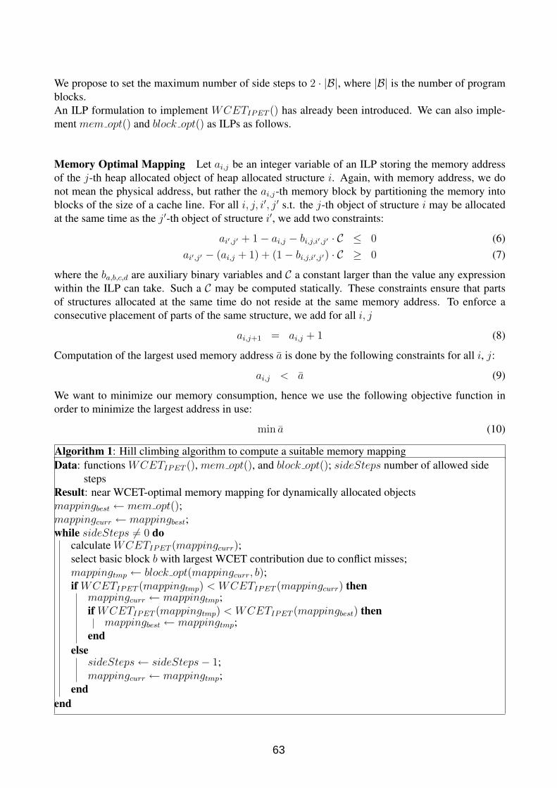
We propose to set the maximum number of side steps to 2 · |B|, where |B| is the number of programblocks.An ILP formulation to implement WCETIPET () has already been introduced. We can also imple-ment mem opt() and block opt() as ILPs as follows.

Memory Optimal Mapping Let ai,j be an integer variable of an ILP storing the memory addressof the j-th heap allocated object of heap allocated structure i. Again, with memory address, we donot mean the physical address, but rather the ai,j-th memory block by partitioning the memory intoblocks of the size of a cache line. For all i, j, i′, j′ s.t. the j-th object of structure i may be allocatedat the same time as the j′-th object of structure i′, we add two constraints:

ai′,j′ + 1− ai,j − bi,j,i′,j′ · C ≤ 0 (6)ai′,j′ − (ai,j + 1) + (1− bi,j,i′,j′) · C ≥ 0 (7)

where the ba,b,c,d are auxiliary binary variables and C a constant larger than the value any expressionwithin the ILP can take. Such a C may be computed statically. These constraints ensure that partsof structures allocated at the same time do not reside at the same memory address. To enforce aconsecutive placement of parts of the same structure, we add for all i, j

ai,j+1 = ai,j + 1 (8)

Computation of the largest used memory address a is done by the following constraints for all i, j:

ai,j < a (9)

We want to minimize our memory consumption, hence we use the following objective function inorder to minimize the largest address in use:

min a (10)

Algorithm 1: Hill climbing algorithm to compute a suitable memory mappingData: functions WCETIPET (), mem opt(), and block opt(); sideSteps number of allowed side

stepsResult: near WCET-optimal memory mapping for dynamically allocated objectsmappingbest ← mem opt();mappingcurr ← mappingbest;while sideSteps 6= 0 do

calculate WCETIPET (mappingcurr);select basic block b with largest WCET contribution due to conflict misses;mappingtmp ← block opt(mappingcurr, b);if WCETIPET (mappingtmp) < WCETIPET (mappingcurr) then

mappingcurr ← mappingtmp;if WCETIPET (mappingtmp) < WCETIPET (mappingbest) then

mappingbest ← mappingtmp;end

elsesideSteps← sideSteps− 1;mappingcurr ← mappingtmp;

endend

63

Block Optimal Mapping To get a block optimal memory mapping with respect to potential conflictcache misses, we modify the ILP used to compute a memory usage optimal mapping as follows. Wefirst compute the cache sets to which memory blocks are mapped that are accessed in the basic blockwe want to optimize the mapping for.Let #cs denote the number of cache sets and csa,i,j denote binary variables set to 1 iff the j-th blockof structure i is mapped to cache set a. The following set of constraints (for each a, i, j, s.t. a isa cache set and block j of structure i is accessed in the considered basic block) sets these csa,i,j

accordingly. However, several auxiliary variables have to be set previously. Let oi,j denote the j-thblock of structure i. Then ai,j stores the cache set to which oi,j is mapped, and ni,j stores the result ofan integer division of the address of oi,j by #cs. Furthermore, ya,i,j is set to |a − csi,j| and ltza,i,j to0 iff a− csi,j < 0.

ai,j − ni,j ·#cs− csi,j = 0 (11)ni,j ≥ 0 (12)csi,j ≥ 0 (13)

csi,j −#cs + 1 ≤ 0 (14)a− csi,j − ltza,i,j · C ≤ 0 (15)

a− csi,j + (1− ltza,i,j) · C ≥ 0 (16)a− csi,j ≤ ya,i,j (17)

− (a− csi,j) ≤ ya,i,j (18)a− csi,j + (1− ltza,i,j) · C ≥ ya,i,j (19)− (a− csi,j) + ltza,i,j · C ≥ ya,i,j (20)

Finally, we assign csa,i,j using the following constraints:

ya,i,j − C · (1− csa,i,j) ≤ 0 (21)ya,i,j − (1− csa,i,j) ≥ 0 (22)

We compute the number of potential cache misses pa resulting from accessing cache set a using thefollowing constraints for all cache sets a; ba being auxiliary binary variables, and k denoting theassociativity of the cache: (∑

i,j

csa,i,j

)− k − ba · C ≤ 0 (23)(∑

i,j

csa,i,j

)− k + (1− ba) · C ≥ 0 (24)

0 ≤ pa (25)(∑i,j

csa,i,j

)− (1− ba) · C ≤ pa (26)

The objective function itself is replaced by

min C ·∑

0≤a<k

pa + a (27)

64

with the intention of minimizing the number of conflict misses that may occur during execution ofthe considered basic block. However, if the number of cache sets increases, the ILP to compute theblock optimal mapping becomes intractable independently of the number of heap objects. Experi-ments suggest that for target hardware with 256 or more cache sets solutions to the ILPs cannot becomputed in reasonable time anymore. Computing block optimal mappings using ILP formulationsalso introduces severe complexity issues for programs with a large number of heap allocated memoryblocks. In order to enable the analysis of larger programs and/or programs for hardware with morecache sets, we propose to replace the block optimal ILP by a heuristic algorithm. Consider a simulatedannealing [5] algorithm as sketched in Algorithm 2. The neighborhood N(m) of a memory mappingm can be defined as the set of all memory mappings, s.t. the address of exactly 1 structure s differsin its address in m by 1. Formally speaking, for a memory mapping m =

⋃oi,j∈O{oi,j 7→ ai,j}, the

neighborhood is defined as N(m) ={m⊕ {oi,j 7→ a′i,j}||ai,j − a′i,j| = 1

}. The evaluation function

to determine the costs of a memory mapping m is defined as

eval(m) = C2 ·memoryConflicts(m) + C · potentialConflictMisses(m) + maxAddr(m)

The first component ensures that memory mappings without memory conflicts are preferred. Thenumber of potential conflict misses is minimized by the second component. For mappings withthe same number of conflict misses, component three favors the ones with minimal memory con-sumption. As maximal temperature we use TemperatureMAX = |O|2. The intention is to haveTemperatureMAX large enough to allow for almost random behavior at the beginning of each restart,converging to a (local) optimum. The current cooling ratio is 1.2−(|I|·restarts).

Although, a memory optimal mapping can be computed by our ILP formulation for most programs,this procedure can be easily replaced by a similar simulated annealing heuristic.

Algorithm 2: Simulated annealing algorithm to compute a suitable block optimal mappingResult: memory mapping with minimal potential conflict misses for program block brestarts← 0;mappingbest ← mem opt();while restarts < RESTARTS do

mappingcurr ← mem opt();Temperature← TemperatureMAX ;while Temperature > TemperatureMIN do

compute the set N(mappingcurr) of neighboring mappings of mappingcurr;foreach mappingtmp ∈ N(mappingcurr) do

if eval(mappingtmp) < eval(mappingbest) thenmappingbest ← mappingtmp;

end

set mappingcurr to mappingtmp with probability eeval(mappingcurr)−eval(mappingtmp)

Temperature ;endTemperature← Temperature · Cooling Ratio;

endrestarts← restarts + 1;

end

65

4. Experiments

Our preliminary experiments consider as target platforms the PowerPC MPC603e and a simpler toyarchitecture (DTA): a 2-way set-associative cache with 2 cache sets. The PowerPC CPU utilizesseparated 4-way set-associative instruction and data caches of 16 KB, organized in 128 cache sets witha cache line size of 32 bytes. At present, no hard real-time applications utilizing dynamic memoryallocation exist for embedded systems. Hence, we lack a collection of real-life programs on whichwe could evaluate our algorithm. We therefore consider a typical textbook example used to motivatethe use of dynamic memory allocation. When transforming one data structure into another, dynamicmemory allocation can lead to a memory consumption smaller than the sum of the memory neededto hold both structures by freeing each component of the first data structure as soon as its contentsare copied to the second structure. Suppose you have a data structure A consisting of n objects andeach object occupies l memory blocks. How much memory is needed to transform this structure intoa structure B with n objects each occupying k memory blocks? Assuming that k ≥ l, a momentsthought reveals that we need n · k + l memory blocks for this transformation. We tried our algorithmon several program descriptions, where data structures consisting of n heap objects are transformedinto other structures consisting of an equal number of objects of larger size (Structure-copy(n)). In allinstances, the computed solution used n · k + l memory blocks. In Structure-copy(3)ex we added anadditional program block to Structure-copy(3) in which the first and the last block of the first structureas well as the last block of the second structure are accessed. On the simplified hardware the memoryoptimal mapping for this program is not WCET-optimal anymore. The new WCET-optimal memoryuses one additional memory address to resolve the potential conflict misses in the additional programblock. Our algorithm successfully discovered that. As a more complex example, consider a programas sketched in Figure 2 (b). Here, allocating all 5 blocks sequentially is memory and WCET-optimalfor the PPC hardware. However, the best memory mapping for our toy hardware would be to allocatethe memory block for data structure 3 before that of structure 2. Again, our algorithm discovers that.

BB1

BB2

BBi

BBi+1

...

......

data structure 1size n blocks

data structure 2size 2n blocks

BB1

BB2

BB3

BB4

data structure 1data structure 2data structure 3

(a) Structure-copy(n) (b) If-branchFigure 2. (Basic-)Block Graph with data accesses for some example programs.

Program (Target) Hardware Memory-/Block-Optimal Algorithm Analysis Time (min/max/avg) msStructure-copy(3) DTA ILP/ILP 23/64/38.5Structure-copy(3) DTA ILP/Simulated Annealing 22/82/49.6Structure-copy(3) PPC603e ILP/ILP 23/79/43.2Structure-copy(3) PPC603e ILP/Simulated Annealing 23/89/43.6

Structure-copy(3)ex DTA ILP/ILP 73/164/100.1Structure-copy(3)ex DTA ILP/Simulated Annealing 29/52/35.7Structure-copy(3)ex PPC603e ILP/ILP 23/32/24.9Structure-copy(3)ex PPC603e ILP/Simulated Annealing 23/30/24.8

If-branch DTA ILP/ILP 43,332/44,005/43,755If-branch DTA ILP/Simulated Annealing 26/35/28.5If-branch PPC603e ILP/ILP 17/41/20.7If-branch PPC603e ILP/Simulated Annealing 17/25/18.4

Structure-copy(100) DTA Simulated Annealing/Simulated Annealing 9,118/9,710/9,362.3Structure-copy(100) PPC603e Simulated Annealing/Simulated Annealing 9,025/9,629/9,345.1Structure-copy(500) PPC603e Simulated Annealing/Simulated Annealing 260,401/276,797/268,932.7

Figure 3. Running times of example analyses each executed 10 times on a 2.66 GHz Core 2 Duo with 2 GB RAM.

66

5. Improvements and Future Work

Our algorithms rely on solving ILPs whose complexity might significantly increase with the numberof data structures or more precisely with the number of ai,j variables. However, many programs allo-cate objects on the heap, although these objects do not survive the function frame they are allocatedin. Hence, such heap objects might be allocated on the stack, in which case they would not contributeto the complexity of our algorithm. Escape analysis is a static analysis that determines which heapallocated objects’ lifetimes are not bounded by the stack frame they are allocated in [1, 3]. By al-locating objects on the stack that do not escape the procedure they are created in, 13% to 95% of aprograms heap data can be moved onto the stack [1]. Incorporating an escape analysis and a programtransformation moving heap objects onto the stack might therefore significantly reduce the complex-ity of our algorithm for real-life programs. Therefore, we are currently developing a novel, preciseescape analysis based on shape analysis via 3-valued logic [9].

6. Conclusions

Transforming dynamic allocation into static allocation circumvents the main problems of WCETanalyses introduced by the unpredictability of memory allocators. Preliminary benchmarks and ex-periments suggest that such a transformation can be computed with reasonable efforts. However,whether it is feasible to fully automate the process of transforming dynamic allocation to static allo-cation, i.e., also automatically generate program descriptions, and at what computational costs stillremains to be seen.

References

[1] B. Blanchet, “Escape Analysis for Object-Oriented Languages: Application to Java,” SIGPLANNot. Vol. 10, 1999.

[2] C. Ferdinand and R. Wilhelm “Efficient and Precise Cache Behavior Prediction for Real-TimeSystems,” Real-Time Systems, 17(2-3):131–181, 1999.

[3] D. Gay and B. Steensgaard, “Fast Escape Analysis and Stack Allocation for Object-Based Pro-grams,” CC’00, 82–93, 2000.

[4] J. Herter, J. Reineke, and R. Wilhelm, “CAMA: Cache-Aware Memory Allocation for WCETAnalysis,” WiP Session of ECRTS’08, 24–27, July 2008.

[5] S. Kirkpatrick, C.D. Gelatt, and M.P. Vecchi, “Optimization by Simulated Annealing,” Science,Number 4598, 671–680, 1983.

[6] M. Langenbach, S. Thesing, and R. Heckmann “Pipeline Modeling for Timing Analysis,” Pro-ceedings of the Static Analyses Symposium (SAS), volume 2477, 2002.

[7] D. Lea, “A Memory Allocator,” Unix/Mail, 6/96, 1996.

[8] Y. S. Li and S. Malik, “Performance Analysis of Embedded Software Using Implicit Path Enu-meration,” Proceedings of the 32nd ACM/IEEE Design Automation Conference, 456–461, 1995.

[9] M. Sagiv, T. Reps, and R. Wilhelm, “Parametric Shape Analysis via 3-valued Logic,” ACM Trans-actions on Programming Languages and Systems, Vol. 24, No. 3, Pages 217–298, May 2002.

[10] M. Schoeberl, “Time-predictable Cache Organization,” STFSSD’09, March 2009.

67

CACHE-RELATED PREEMPTION DELAYCOMPUTATION FOR SET-ASSOCIATIVE CACHES

PITFALLS AND SOLUTIONS

Claire Burguiere, Jan Reineke, Sebastian Altmeyer1

AbstractIn preemptive real-time systems, scheduling analyses need—in addition to the worst-case executiontime—the context-switch cost. In case of preemption, the preempted and the preempting task mayinterfere on the cache memory. These interferences lead to additional reloads in the preempted task.The delay due to these reloads is referred to as the cache-related preemption delay (CRPD). TheCRPD constitutes a large part of the context-switch cost. In this article, we focus on the computationof upper bounds on the CRPD based on the concepts of useful cache blocks (UCBs) and evicting cacheblocks (ECBs). We explain how these concepts can be used to bound the CRPD in case of direct-mapped caches. Then we consider set-associative caches with LRU, FIFO, and PLRU replacement.We show potential pitfalls when using UCBs and ECBs to bound the CRPD in case of LRU anddemonstrate that neither UCBs nor ECBs can be used to bound the CRPD in case of FIFO andPLRU. Finally, we sketch a new approach to circumvent these limitations by using the concept ofrelative competitiveness.

1. Introduction

Preemption introduces a new dimension of complexity into worst-case execution time (WCET) anal-ysis: The possible interference of preempting and preempted task – especially on the cache – has tobe taken into account. The additional execution time due to preemption is referred to as the context-switch cost (CSC), the part of the context switch cost due to cache interferences as cache-relatedpreemption delay (CRPD). One approach to soundly deal with cache interferences due to preemptionis to totally avoid them by cache partitioning. When cache partitioning is not an option, one can dis-tinguish two other approaches: 1) to incorporate cache interferences within WCET analysis, or 2) toperform a separate analysis of the number of additional misses due to preemption. Whereas only thefirst alternative is applicable to processors exhibiting timing anomalies, the second one is probablymore precise but relies on “timing compositional” processors.

Lee et al. [2] laid the foundation for the separate analysis of the cache-related preemption delay byintroducing the notion of useful cache block (UCB). A cache block of the preempted task is calleduseful at program point P , if it may be cached at P and if it may be reused at some program pointreached from P . Memory blocks that meet both criteria may cause additional cache misses that onlyoccur in case of preemption. Hence, an upper bound on the number of UCBs gives an upper boundon the number of additional misses and, multiplied by the cache miss penalty, an upper bound on thecache-related preemption delay.

1Compiler Design Lab, Saarland University, 66041 Saarbrucken, Germany{burguiere,reineke,altmeyer}@cs.uni-saarland.de

68

As Tan et al. [7] and, later, Staschulat et al. [6] have shown, the CRPD bound can be reduced by takinginto account the preempting task. Only those cache blocks that are actually evicted due to preemptionmay contribute to the CRPD. So, the preempting task is analyzed in order to derive the set of evictingcache blocks (ECBs) and to bound the effect of the preempting task on the useful cache blocks. Theseconcepts have been introduced for direct-mapped and set-associative caches with LRU replacement.Although widely used in practice, other replacement policies, such as PLRU or FIFO, have not beenconsidered so far – except for [6] which suggests to adapt the CRPD computation for LRU to PLRU.

We first review how the CRPD can be bounded for direct-mapped caches. Then, we discuss CRPDcomputation for set-associative caches. We show that neither the number of UCBs nor the number ofECBs can be used to bound the CRPD for set-associative caches. Even for LRU, the previously pro-posed combination of ECBs and UCBs may underestimate the CRPD. We provide a correct formulafor LRU and sketch a new approach to CRPD computation for FIFO, PLRU, and other policies.

1.1. Background: Cache Memory

Caches are fast and small memories storing frequently used memory blocks to close the increasingperformance gap between processor and main memory. They can be implemented as data, instructionor combined caches. An access to a memory block which is already in the cache is called a cache hit.An access to a memory block that is not cached, called a cache miss, causes the cache to load andstore the data from the main memory.

Caches are divided into cache lines. Cache lines are the basic unit to store memory blocks, i.e., line-size l contiguous bytes of memory. The set of all memory blocks is denoted by M . The cache sizes is thus given by the number of cache lines c times the line-size l. A set of n cache lines forms onecache set, where n is the associativity of the cache and determines the number of cache lines a specificmemory block may reside in. The number of sets is given by c/n and the cache set that memory blockb maps to is given by b mod(c/n).

Special cases are direct-mapped caches (n = 1) and fully-associative caches (n = c). In the first case,each cache line forms exactly one cache set and there is exactly one position for each memory block.In the second case, all cache lines together form one cache sets and all memory blocks compete for allpositions. If the associativity is higher than 1 a replacement policy has to decide in which cache lineof the cache set a memory block is stored, and, in case all cache lines are occupied, which memoryblock to remove. The goal of the replacement policy is to minimize the number of cache misses.

We will investigate CRPD computation in the context of the following three widely-used policies:• Least-Recently-Used (LRU) used in INTEL PENTIUM I and MIPS 24K/34K

• First-In, First-Out (FIFO or Round-Robin) used in MOTOROLA POWERPC 56X,INTEL XSCALE, ARM9, ARM11

• Pseudo-LRU (PLRU) used in INTEL PENTIUM II-IV and POWERPC 75X

We will explain these policies in Section 3.

2. Bounding the CRPD for direct-mapped caches

The cache-related preemption delay denotes the additional execution time due to cache misses causedby a single preemption. Such cache misses occur, if the preempting task evicts cache blocks of the

69

preempted task that otherwise would later be reused. Therefore upper bounds on the CRPD can bederived from two directions: bounding the worst-case effect on the preempted task or bounding theeffect of the preempting task. Note that the schedulability analysis might have to account for multiplepreemptions. In that case, it has to multiply the CRPD bound by the number of preemptions.

For the analysis of the preempted task, Lee et al. [2] introduced the concept of useful cache blocks:

Definition 1 (Useful Cache Block (UCB))A memory block m is called a useful cache block at program point P , if

a) m may be cached at P

b) m may be reused at program point Q that may be reached from P without eviction of m on thispath.

In case of preemption at program point P , only the memory blocks that a) are cached and b) will bereused, may cause additional reloads. Hence, the number of UCBs at program point P gives an upperbound on the number of additional reloads due to a preemption at P . A global bound on the CRPDof the whole task is determined by the program point with the highest number of UCBs.

The worst-case effect of the preempting task is given by the number of cache blocks the task mayevict during preemption. Obviously, each memory block possibly cached during the execution of thepreempting task may evict a cache block of the preempted one:

Definition 2 (Evicting Cache Blocks (ECB))A memory block of the preempting task is called an evicting cache block, if it may be accessed duringthe execution of the preempting task.

Accessing an ECB in the preempting task may evict a cache block of the preempted task. Tomiyamaand Dutt [8] proposed to use only the number of ECBs – in a more precise manner – to bound theCRPD. Negi et al. [3] and Tan et al. [7] proposed to combine the number of ECBs and UCBs toimprove the CRPD bounds; only useful cache blocks that are actually evicted by an evicting cacheblock may contribute to the CRPD.

Hence, the following three formulas can be used to bound the CRPD for direct-mapped caches (wherec denotes the number of cache sets):

CRPDUCB = CRT · |{si | ∃m ∈ UCB : m mod c = si}| (1)

The CRPD is bounded by the cache reload time (CRT) times the number of sets, which at least oneUCB maps to [2].

CRPDECB = CRT · |{si | ∃m ∈ ECB : m mod c = si}| (2)

The CRPD is bounded by the cache reload time times the number of sets, which at least one ECBmaps to [8].

CRPDUCB&ECB = CRT · |{si | ∃m ∈ UCB : m mod c = si ∧ ∃m′ ∈ ECB : m′ mod c = si}| (3)

The CRPD is bounded by the cache reload time times the number of sets, which at least one UCB andone ECB map to [3, 7].

The computation of UCBs and ECBs is out of the scope of this paper. Detailed information can befound in the original paper [2], as well as in [3, 6].

70

0x080x090x0a0x0b

Without preemption:

[b, a, 9, 8] 8 [8, b, a, 9] 9 [9, 8, b, a]a

[a, 9, 8, b] b [b, a, 9, 8] 0 misses

With preemption:

[e, b, a, 9] 8∗ [8, e, b, a] 9∗ [9, 8, e, b] a∗ [a, 9, 8, e] b∗ [b, a, 9, 8] 4 misses

ECBs= {e}

Figure 1. Evolution of the cache contents for LRU replacement. The first row shows the evolution of the cachecontents accessing 8, 9, a, b without preemption. The second row shows the evolution of the cache contents on thesame sequence with preemption. Preempting task accesses block e that maps to this cache set. Each miss is markedby ∗. Blocks 8, 9, a and b are useful before this access sequence.

3. Bounding the CRPD for set-associative instruction caches

The definitions of UCBs and ECBs apply to all types of cache architectures, including set-associativecaches with any replacement policy. Of course, whether a block is useful or not depends on theparticular cache architecture, i.e., its associativity and replacement policy. So, a UCB analysis needsto be tailored to a specific cache architecture. In addition, for set-associative caches, the CRPDcomputation based on UCBs and ECBs differs from one replacement policy to another. As we showin this section, several pitfalls may be encountered on the way to the CRPD computation for the mostcommon replacement policies LRU, FIFO, and PLRU.

3.1. LRU – Least-Recently-Used

Least-Recently-Used (LRU) policy replaces the least-recently-used element on a cache miss. It con-ceptually maintains a queue of length k for each cache set, where k is the associativity of the cache.In the case of LRU and associativity 4, [b, c, e, d] denotes a cache set, where elements are orderedfrom most- to least-recently-used. If an element is accessed that is not yet in the cache (a miss), it isplaced at the front of the queue. The last element of the queue, i.e., the least-recently-used, is thenremoved if the set is full. In our example, an access to f would thus result in [f, b, c, e]. Upon a cachehit, the accessed element is moved from its position in the queue to the front, in this respect treatinghits and misses equally. Accessing c in [f, b, c, e] results in [c, f, b, e].

Since we concentrate on the use rather than on the computation of UCBs, we refer to Lee et al. [2] andStaschulat et al. [6] in case of LRU. For the derivation of the CRPD, there are again three possibilities:UCBs, ECBs and the combination of both.

The cache state after preemption may cause additional cache misses compared with the cache statewithout preemption. However the difference in the number of misses, and thus, the number of ad-ditional reloads, per cache set is always bounded by the associativity n: This is because any twoinitially different cache-set states converge within n accesses for LRU [4]. In particular, this holdsfor the cache states after preemption and the cache state without preemption. Furthermore, the num-ber of additional misses is bounded by the number of reused memory blocks. Thus, the number ofUCBs bounds the additional cache misses.

However, due to control flow joins in the UCB analysis, the number of UCBs per set may exceed the

71

associativity of the cache. Therefore, we have to limit the number of UCBs per set to n:

CRPDLRUUCB = CRT ·

c∑s=1

min(|UCB(s)|, n) (4)

where UCB(s) denotes the set of UCBs mapping to cache set s.By using solely the number of ECBs to bound the CRPD, a more complex formula is needed. Asshown in Figure 1, a single ECB may cause up to n additional cache misses in the set it maps to.Therefore, the number of additional cache misses for set s (CRPDLRU

ECB (s)) is zero, in case no ECBmaps to set s, and, otherwise, bounded by the associativity (n) of the cache.

CRPDLRUECB =

c∑s=1

CRPDLRUECB (s) (5)

where

CRPDLRUECB (s) =

{0 if ECB(s) = ∅CRT · n otherwise (6)

where ECB(s) denotes the set of ECBs mapping to cache set s.To bound the number of additional reloads for cache set s using both UCBs and ECBs, Tan et al. [7]proposed the minimum function on the number of UCBs, the number of ECBs and the number ofways:

CRPDLRUMIN (s) = CRT ·min(|UCB(s)|, |ECB(s)|, n) (7)

where UCB(s) and ECB(s) denote the sets of UCBs and ECBs, respectively, mapping to cache set s.

However, this function gives an underestimation on the number of misses in several cases. Considerthe CFG of Figure 1. The memory blocks all map to the same cache set. Therefore, at the end of theexecution of this basic block, the content of the 4-way set is given by [b, a, 9, 8]. As this basic blockforms the body of a loop, these memory blocks are useful. One block of the preempting task mapsto this set and evicts only one useful cache block: Using the minimum function, only one additionalmiss is taken into account for this memory set (min(4, 1, 4) = 1). However, the number of additionalmisses, 4, is greater than the number of ECBs, 1: All useful cache blocks are evicted and reloaded.In this example, the number of UCBs and the number of ways are upper bounds on the number ofmisses, but the minimum function results in an underestimation of the CRPD.

Instead of using the formula by Tan et al., the results from the CRPD computation via UCB and viaECB can be combined in a straight-forward manner:

CRPDLRUUCB&ECB =

c∑i=1

CRPDLRUUCB&ECB(s) (8)

where

CRPDLRUUCB&ECB(s) =

{0 if ECB(s) = ∅CRT ·min(|UCB(s)|, n) otherwise (9)

Again, UCB(s) and ECB(s) denote the sets of UCBs and ECBs, respectively, mapping to cache set s.If no ECB maps to cache set s, no additional cache misses occur – as in Equation 6. Otherwise, thenumber of additional cache misses is bounded by the number of UCBs and the associativity of thecache – as in Equation 4.

72

3.2. FIFO – First-In, First-Out

First In, First Out (FIFO, also known as Round-Robin) bases its replacement decisions on when anelement entered the cache, not on the time of its most-recent use. It replaces the element which hasbeen resident in the cache for the longest time. FIFO cache sets can also be seen as a queue: newelements are inserted at the front evicting elements at the end of the queue. This resembles LRU. Incontrast to LRU, hits do not change the queue. In our representation of FIFO cache sets, elementsare ordered from last-in to first-in: Assume an access to f . In [b, c, e, d], d will be replaced on a miss,resulting in [f, b, c, e].

Without preemption: [b, a]a

[b, a] e∗ [e, b] b [e, b] c∗ [c, e]e

[c, e] 2 misses

With preemption: [x, b] a∗ [a,x] e∗ [e, a] b∗ [b, e] c∗ [c, b] e∗ [e, c] 5 misses

ECBs= {x}

Figure 2. Evolution of the cache contents for FIFO replacement. The first row shows the evolution of the cachecontents accessing a, e, b, c, e without preemption. The second row shows the evolution of the cache contents on thesame sequence with preemption. Each miss is marked by ∗. Blocks a and b are useful before this access sequence.

The definitions of UCBs and ECBs also apply to FIFO caches. However, there is no correlationbetween the number of additional misses due to preemption and the number of UCBs, the numberof ECBs or the number of ways. We illustrate this using the example of Figure 2. Consider a 2-wayset-associative FIFO cache. The preemption occurs before the presented sequence: Blocks a andb are useful, memory block a is evicted and the final content of this set after preemption is [x, b].The number of misses in the case without preemption is 2 and it is 5 in the case of preemption. Thenumber of additional misses, 3, is greater than the number of UCBs, 2, the number of ways, 2, and thenumber of ECBs, 1. So, these numbers cannot be used as an upper bound on the number of additionalmisses when FIFO replacement is used.

3.3. PLRU – Pseudo-LRU

Pseudo-LRU (PLRU) is a tree-based approximation of the LRU policy. It arranges the cache lines atthe leaves of a tree with k−1 “tree bits” pointing to the line to be replaced next; a 0 indicating the leftsubtree, a 1 indicating the right. After every access, all tree bits on the path from the accessed line tothe root are set to point away from the line. Other tree bits are left untouched. Consider the followingexample of 3 consecutive accesses to a set of a 4-way set-associative PLRU cache:

1

1 0

a b c d

e* 0

1 1

a b e d

a 1

1 1

a b e d

f* 0

1 0

a b e f

The first access in the sequence, to e, is a miss. It replaces c, which is pointed to by the tree bits. Thetree bits on the path from e to the root of the tree are flipped to protect e from eviction. The secondaccess in the sequence, to a, is a hit. The left tree bit already points away from a, so only the root treebit is flipped. Another access to a would not change the tree bits at all. Finally, the access to f , isanother miss, replacing d.

As for FIFO replacement, the definition of UCB applies to the PLRU replacement strategy; but thenumber of UCBs, the number of ECBs and the number of ways are not upper bounds on the number

73

of additional misses due to preemption. This is shown in Figure 3. There are two accesses to this setduring the execution of the preempting task: Block b and d are evicted by x and y. The number ofUCBs, 4, the number of ECBs, 2, and the number of ways, 4, are lower than the number of additionalmisses, 5. Thus, to compute an upper bound on the CRPD, one cannot use these numbers to derive animmediate upper bound on the number of additional cache misses.

Without preemption:

1

1 1

a b c d

d 0

1 0

a b c d

b 1

0 0

a b c d

c 0

0 1

a b c d

b 1

0 1

a b c d

a 1

1 1

a b c d

d 0

1 0

a b c d

0 misses

With preemption:

1

0 0

a y c x

d* 0

0 1

a y d x

b* 1

1 1

b y d x

c* 0

1 0

b y d c

b 1

1 0

b y d c

a* 0

1 1

b y a c

d* 1

0 1

b d a c

5 misses

ECBs= {x,y}

Figure 3. Evolution of the cache contents for PLRU replacement. The first row shows the evolution of the cachecontents accessing d, b, c, b, a, d without preemption. The second row shows the evolution of the cache contents onthe same sequence with preemption. Each miss is marked by ∗. Blocks a, b, c and d are useful before this accesssequence.

For both FIFO and PLRU, we can extend the access sequences of our examples in Figures 2 and 3such that the number of additional misses grows arbitrarily. In general, policies whose miss-sensitivityis greater than 1 exhibit such problems [4].

4. A new approach for FIFO, PLRU, and other policies

In the previous section, we have seen that the number of UCBs and the number of ECBs cannot beused to bound the CRPD for FIFO and PLRU. In this section, we sketch a new approach to the CRPDcomputation for policies other than LRU, including FIFO and PLRU. Due to space limitations, wecannot provide correctness proofs of the proposed approaches. Our basic idea is to transform guaran-tees for LRU to guarantees for other policies. To this end, we make use of the relative competitivenessof replacement policies:

4.1. Relative Competitiveness

Relative competitive analyses yield upper bounds on the number of misses of a policy P relative tothe number of misses of another policy Q. For example, a competitive analysis may find out thatpolicy P will incur at most 30% more misses than policy Q in the execution of any task.

For the definition of relative competitiveness we need the following notation: mP (p, s) denotes thenumber of misses of policy P on access sequence s ∈ M∗ starting in state p ∈ CP . M denotes theset of memory blocks and CP the set of states of policy P . For the precise definition of compatible,we refer the reader to [5]. Intuitively, it ensures that the policies are not given an undue advantage bythe starting state.

Definition 3 (Relative Miss-Competitiveness)A policy P is (k, c)-miss-competitive relative to policy Q, if

mP (p, s) ≤ k ·mQ(q, s) + c

for all access sequences s ∈M∗ and compatible cache-set states p ∈ CP , q ∈ CQ.

74

In other words, policy P will incur at most k times the number of misses of policy Q plus a constant con any access sequence. For a pair of policies P and Q, there is a smallest k, such that P is k-miss-competitive relative to Q. This is called the relative competitive ratio of P to Q. Relative competitiveratios can be computed automatically for a pair of policies [5]2.

The competitiveness of FIFO and PLRU relative to LRU has been studied in [4, 5]. The mostimportant results in our context are (the numbers in parentheses denote the associativities of thepolicies):

• PLRU(k) is (1, 0)-miss-competitive relative to LRU(1 + log2k).

• FIFO(k) is ( kk−l+1

, l)-miss-competitive relative to LRU(l).

This means that a PLRU-controlled cache of associativity k always performs at least as good as anLRU-controlled cache of associativity 1 + log2k with the same number of cache sets. In contrast toPLRU, it is not possible to achieve (1, 0)-miss-competitive relative to LRU for FIFO. However, thegreater the associativity of FIFO is relative to the associativity of LRU, the closer k

k−l+1gets to 1.

The relative competitiveness results mentioned above are for fully-associative caches. However, theycan easily be lifted to set-associative caches, which can be seen as the composition of a number offully-associative sets. If P is (k, c)-miss-competitive relative to Q in the fully-associative case, it is(k, c · s)-miss-competitive relative to Q for a set-associative cache with s cache sets.

4.2. WCET and CRPD computation based on Relative Competitiveness

We have seen in the previous section that neither the number of UCBs nor the number of ECBs canbe used to bound the CRPD for FIFO and PLRU. Our approach relies on the following observation:WCET and CRPD are always used in combination by schedulability analysis. For schedulabilityanalysis it is sufficient, if (WCET bound + n·CRPD estimate) is greater than the execution time ofthe task including the cost of n preemptions. In that case, for safe schedulability analysis, the CRPDestimate alone does not have to bound the real CRPD. Recent work on CRPD computation providesonly this weaker guarantee [1]. In addition, all sound existing approaches [2, 6] for LRU naturallyalso fulfill this weaker guarantee. For FIFO and PLRU, this allows us to compute a CRPD estimatethat is not necessarily a bound on the CRPD itself: We will compute the WCET bound and CRPDestimate in such a way that together they provide the guarantee described above. The idea behind theapproach we will present is to adapt WCET and CRPD analyses, which were originally designed forLRU, to other policies.

The CRPD accounts for all additional reloads due to preemption. Memory accesses that cause ad-ditional reloads due to preemption might have been considered to be hits by the WCET analysis,which assumes uninterrupted execution. The sequence of memory accesses along the execution ofthe preempted task can be split into two subsequences: the sequence of memory accesses before thepreemption point and the sequence after it. Figure 4 illustrates this situation. First we consider anuninterrupted task execution. Then, mpre and mpost denote the number of misses on the sequencesbefore and after the preemption point. For the interrupted execution, mpre and mpost denote the num-ber of misses on the same sequences including the effects of the preemption. As the execution of thefirst sequence is not influenced by the preemption, mpre and mpre are equal. mCRPD is the number ofadditional misses due to preemption. So, mpost is the sum of mpost and mCRPD. The total number ofmisses on the sequence is given by: m = mpre + mpost = mpre + (mpost + mCRPD) = m + mCRPD.

2See http://rw4.cs.uni-sb.de/˜reineke/relacs for an applet that computes relative competitive ratios.

75

(a)

mpre = 4 mpost = 2

(b)

mpre = mpre = 4 mpost = mpost + mCRPD = 5

Figure 4. Sequence of memory accesses during task execution without preemption (a) and with preemption (b).© represents a miss, × a hit and ⊗ an additional miss due to preemption.

For each of the two sequences, relative competitiveness allows to transfer the number of misses forone policy to a bound of a number of misses for another policy. Let policy P(t) be (k, c)-miss-competitive relative to LRU(s), and let mP(t) and mLRU(s) denote the number of misses of the twopolicies. Then,

mP(t)pre ≤ k ·mLRU(s)

pre + c and mP(t)post ≤ k ·mLRU(s)

post + c

= k ·mLRU(s)pre + c = k · (mLRU(s)

post + mLRU(s)CRPD ) + c.

So, the total number of misses of policy P(m) can also be bounded by the number of misses ofLRU(s):

mP(t) = mP(t)pre + m

P(t)post

≤ k ·mLRU(s)pre + c + k · (mLRU(s)

post + mLRU(s)CRPD ) + c

= (k · (mLRU(s)pre + m

LRU(s)post ) + c) + (k ·mLRU(s)

CRPD + c)

= (k ·mLRU(s) + c) + (k ·mLRU(s)CRPD + c).

We can split this bound into mP(t) = k · mLRU(s) + c and mP(t)CRPD = k · mLRU(s)

CRPD + c, such thatmP(t) ≤ mP(t) + m

P(t)CRPD. Note that while we do obtain a bound on the number of misses for P(t)

including the preemption, namely mP(t) + mP(t)CRPD, we do not necessarily obtain a bound on the

cache-related preemption delay for P(t), i.e. mP(t)CRPD itself does not bound the real CRPD.

WCET and CRPD analyses take into account all possible access sequences. Our calculations aboveconsidered a single access sequence. However, the result can be lifted to all possible access sequencesby considering bounds on the number of additional misses (CRPD) and bounds on the number ofmisses during task execution. Also, we have considered exactly one preemption in our calculations.However, it can be verified rather easily, that mP(t) + n ·mP(t)

CRPD is a bound on the number of missesfor P(t) including up to n preemptions by similar calculations as above.

What does all this mean for the WCET and CRPD analysis of FIFO and PLRU? Due to its (1, 0)-miss-competitive relative to LRU(1 + log2k), PLRU(k) is particularly easy to treat: One can simplyperform WCET and CRPD analyses assuming an LRU(1 + log2k) cache. The resulting bounds willalso be valid for PLRU(k). The situation becomes more difficult for FIFO. It is not (1, 0)-miss-competitive relative to LRU(k) for any associativity. FIFO(k) is ( k

k−l+1, l)-miss-competitive relative

76

to LRU(l). To handle FIFO correctly, both the WCET and the CRPD analyses need to be adapted.m

FIFO(k)CRPD = k

k−l+1·mLRU(l)

CRPD + l can be used as a CRPD estimate for FIFO(k) given that mLRU(l)CRPD is a

sound estimate for LRU(l). Likewise, the WCET analysis for FIFO(k) needs to account for kk−l+1

as many misses as it would have to for LRU(l) plus l misses. For WCET analyses that explicitlycompute an upper bound on the number of cache misses, like ILP-based approaches, this can berather easily. Other WCET analyses that take cache misses into account as part of the execution timeof basic blocks it maybe more difficult to account for the higher number of misses.

5. Conclusions and Future Work

Prior useful cache block analyses mainly focus on direct-mapped caches. They use the number ofUCBs and/or ECBs to derive an upper-bound on the CRPD. As we have shown in this paper, con-sidering set-associative caches, the CRPD computation is much more complex. In case of LRUreplacement, the computation of the CRPD solely based on the number of UCBs is correct, whereasa previously proposed formula combining UCBs and ECBs may underapproximate the CRPD. Incontrast to LRU, for PLRU and FIFO policies, neither UCBs nor ECBs can be used to bound theCRPD.

For LRU, we introduce a new CRPD formula based on UCBs and ECBs. For other policies, wesketch a new approach to bound the CRPD. This approach is based on the concept of relative compet-itiveness: Bounds obtained for LRU are transformed into bounds for other policies. For future workwe plan to implement and experimentally evaluate this approach.

References

[1] Sebastian Altmeyer and Claire Burguiere. A new notion of useful cache block to improve thebounds of cache-related preemption delay. In ECRTS’09, 2009.

[2] Chang-Gun Lee, J. Hahn, Sang Lyul Min, R. Ha, Seongsoo Hong, Chang Yun Park, Minsuk Lee,and Chong Sang Kim. Analysis of cache-related preemption delay in fixed-priority preemptivescheduling. In RTSS’96, page 264, Washington, DC, USA, 1996. IEEE Computer Society.

[3] Hemendra Singh Negi, Tulika Mitra, and Abhik Roychoudhury. Accurate estimation of cache-related preemption delay. In CODES+ISSS’03, New York, NY, USA, 2003. ACM.

[4] Jan Reineke. Caches in WCET Analysis. PhD thesis, Universitat des Saarlandes, Saarbrucken,November 2008.

[5] Jan Reineke and Daniel Grund. Relative competitive analysis of cache replacement policies. InLCTES’08, pages 51–60, New York, NY, USA, June 2008. ACM.

[6] Jan Staschulat and Rolf Ernst. Scalable precision cache analysis for real-time software. ACMTrans. on Embedded Computing Sys., 6(4):25, 2007.

[7] Yudong Tan and Vincent Mooney. Integrated intra- and inter-task cache analysis for preemptivemulti-tasking real-time systems. In SCOPES’04, pages 182–199, 2004.

[8] Hiroyuki Tomiyama and Nikil D. Dutt. Program path analysis to bound cache-related preemptiondelay in preemptive real-time systems. In CODES’00, New York, NY, USA, 2000. ACM.

77

WCET-AWARE SOFTWARE BASED CACHEPARTITIONING FOR MULTI-TASK REAL-TIME

SYSTEMS 1

Sascha Plazar2, Paul Lokuciejewski2, Peter Marwedel2

AbstractCaches are a source of unpredictability since it is very difficult to predict if a memory access resultsin a cache hit or miss. In systems running multiple tasks steered by a preempting scheduler, it iseven impossible to determine the cache behavior since interrupt-driven schedulers lead to unknownpoints of time for context switches. Partitioned caches are already used in multi-task environments toincrease the cache hit ratio by avoiding mutual eviction of tasks from the cache.

For real-time systems, the upper bound of the execution timeis one of the most important metrics,called the Worst-Case Execution Time (WCET). In this paper, we use partitioning of instruction cachesas a technique to achieve tighter WCET estimations since tasks can not be evicted from their partitionby other tasks. We propose a novel WCET-aware cache partitioning algorithm, which determines theoptimal partition size for each task with focus on decreasingthe system’s WCET for a given set ofpossible partition sizes. Employing this algorithm, we are able to decrease the WCET depending onthe number of tasks in a set by up to 34%. On average, reductions between 12% and 19% can beachieved.

1 Introduction

Embedded systems often operate as hard real-time systems which have to meet hard timing con-straints. For these systems, it is mandatory to know the upper bound of the execution time for eachtask and possible input data. This bound is calledWorst-Case Execution Time.

Caches have become popular to bridge the gap between high processor and low memory performance.The latency for an access to a certain memory address highly depends on the content of the cache. Ifan instruction to be fetched already resides in the cache, then a so calledcache hitoccurs and the fetchcan be usually performed within one cycle. Otherwise, it results in acache miss. The desired addresshas to be fetched from the slow main memory (e.g. Flash) leading to penalty cycles depending on theprocessor and memory architecture.

It is hard to determine statically if an arbitrary memory access results in a cache hit or a cache miss.However, caches are used in real-time systems because they can drastically speed up the executionof programs. Hence, a lot of effort has been successfully putinto research to make sound predictionabout the worst-case cache performace during a program’s execution. AbsInt’saiT [2] is a tool thatperforms static analyses on binary programs to predict their cache behavior and WCET.

1The research leading to these results has received funding from the European Community’s ArtistDesign Network ofExcellence and from the European Community’s Seventh Framework Programme FP7/2007-2013 under grant agreementno 216008.

2Computer Science 12 — TU Dortmund University — D-44221 Dortmund, Germany — FirstName.LastName@tu-dortmund.de

78

In environments with preemptive schedulers running more than one task, it is impossible to make anyassumption about the memory access patterns. This is mainlycaused by interrupt-driven schedulingalgorithms causing context switches at unknown points of time. Thus, the program’s state in notknown at which a context switch occurs. It is also unknown at which address the execution of aprogram continues, hence it is unknown which line of the cache is evicted next. An unknown cachebehavior forces to assume a cache miss for every memory access implying a highly overestimatedsystems overall WCET. As a consequence, the underlying systemhas to be oversized to meet real-time constraints resulting in higher costs for hardware.

We adapt an existing technique called software based cache partitioning [16] to make the instructioncache (I-cache) behavior more predictable. This can be guaranteed since every task has its owncache partition from which it can not be evicted by another task. Our novel WCET-aware cachepartitioning aims at selecting the optimal partition size for each task of a set to achieve the optimalWCET minimization. The main contributions of this paper are asfollows:

1. Compared to existing approaches which focus on minimization of average-case execution times,our WCET-aware cache partitioning explicitly evaluates WCET data as metric for optimization.

2. In contrast to previous works which presented theories topartition a cache in software, ourapproach comprises a fully functional implementation of a cache partitioning method.

3. We show that our ILP-based WCET-aware cache partitioning iseffective in minimizing a sys-tem’s WCET and outperforms existing algorithms.

The paper is organized as follows: In the next section, we present related work. Existing techniquesto partition a cache as well as our new algorithm are explained in Section 3. Section 4 introducesthe compiler WCC used to integrate our novel cache partitioning algorithm. An evaluation of theperformance which is achieved by our WCET-aware cache partitioning, is presented in Section 5.Finally, we conclude our work and give a brief overview of future work.

2 Related Work

The papers [16, 5, 15] present different techniques to exploit cache partitioning realized either inhardware or in software. In contrast to our work, these implementations either do not take the impacton the WCET into account or do not employ the WCET as the key metric for optimization whichleads to suboptimal or even degraded results. In [16], the author presents ideas for compiler supportfor software based cache partitioning which serves as basisfor the partitioning techniques presented inthis paper. Compared to the work in this paper, a functional implementation or impacts on the WCETare not shown. In [5], a hardware extension for caches is proposed to realize a dynamic partitioningthrough a fine grained control of the replacement policy via software. Access to the cache can berestricted to a subset of the target cache set which is calledcolumnization. For homogeneous on-chipmulti-processor systems sharing a unified set-associativecache, [15] presents partitioning schemesbased on associativity and sets.

A combination of locking and partitioning of shared caches on multi-core architectures is researchedin [18] to guarantee a predictable system behavior. Even tough the authors evaluate the impact of theircaching schemes on the worst-case application performance, their algorithms are not WCET-aware.Kim et al. [11] developed an energy efficient partitioned cache architecture to reduce the energy peraccess. A partitioned L1-cache is used to access only one sub-cache for every instruction fetch leadingto dynamic energy reduction since other sub-caches are not accessed.

79

The authors of [4] show the implications of code expanding optimizations on instruction cache design.Different types of optimizations and their influence on different cache sizes are evaluated. [12] givesan overview of cache optimization techniques and cache-aware numerical algorithms. It focuses onthe bottleneck memory interface which often limits the performance of numerical algorithms.

Puaut et al. counteract the problem of unpredictability with locked instruction caches in multi-taskreal-time systems. They propose two low complexity algorithms for cache content selection in [17].A drawback of statically locking the cache content is that the dynamic behavior of the cache gets lost.Code is no more automatically loaded into the cache, thus codewhich is not locked into the cache cannot profit from it anymore.

Vera et al. [22] combine cache partitioning, dynamic cache locking and static cache analysis of datacaches to achieve predictability in preemptive systems. This eliminates overestimation and allows toapproximate the worst-case memory performance.

Lokuciejewski et. al rearrange the orders of procedures in main memory to exploit locality in thecontrol flow leading to a higher cache performance [13]. Worst-case calling frequencies serve asmetrics for WCET minimization but multi-task sets are not supported.

3 WCET-aware Cache Partitioning

Caches have become popular to bridge the growing gap between processor and memory performancesince they are transparent from the programmer’s point of view. Unfortunately, caches are a source ofunpredictability because it is very difficult to determine if a memory access results in a cache hit ora cache miss. Static analysis is a technique to predict the behavior of the cache [19] and make soundprediction about the WCET of a program which allows the profitable usage of caches in real-timesystems running a single task.

In general, real-time systems consist of more than one task which makes it often impossible to de-termine the worst-case cache behavior. Due to interrupt driven schedulers, points of time for contextswitches can not be statically determined. Thus, it is not predictable which memory address is fetchedfrom the next task being executed and one can not make proven assumptions which cache line is re-placed by such an unknown memory access. Due to this fact, every memory access has to be treatedas a cache miss leading to a highly overestimated WCET caused byan underestimated cache perfor-mance.

In a normally operating cache, each task can be mapped into any cache line depending on its memoryusage. To overcome this situation, partitioned caches are recommended in literature [16, 5, 15].Tasks in a system with partitioned caches can only evict cache lines residing in the partition theyare assigned to. Reducing the prediction problem of replacedcache lines to one task with its owncache partition, allows the application of well known single task approaches for WCET- and cacheperformance estimation. The overall execution time of a task set is then composed of the executiontime of the single tasks with a certain partition size and theoverhead required for scheduling includingadditional time for context switches.

Infineon’s TriCore architecture does not support partitioned caches in hardware so that partitioninghas to be done in software. The following section describes the basics of software based cache parti-tioning schemes applied in our WCET-aware cache partitioningalgorithms. In Section 3.2, a heuristicapproach is applied to determine the partitioning based on the tasks’ sizes. Section 3.3 presents ournovel algorithm for selecting an optimal partition size w.r.t. the overall WCET of a system.

80

3.1 Software based Cache Partitioning

The author in [16] presents a theory to integrate software based cache partitioning into a compilertoolchain without an existing implementation. Code should be scattered over the address space sothat tasks are mapped to certain cache lines. Therefore, alltasks have to be linked together in onemonolithic binary and a possible free space between severalparts has to be filled withNOPs. Parti-tioning for data caches involves code transformation of data references.

Line 0

Line 2

Line 16

Tag

Index Offset

Memory Address

Cache

Tag04831

Line 1

016

Figure 1: Addressing of cache content

The theory to exactly position code in the address spaceto map it into certain cache lines is picked up here, buta completely different technique is applied to achievesuch a distribution. We restrict ourselves to partition-ing of I-caches, thus only software based partitioning ofcode using the new technique is discussed. However,a partitioning of data caches w.r.t. WCET decrease isstraightforward using a modified version of our algo-rithm.

For the sake of simplicity, in the following we assumea direct-mapped cache. Way associative caches can be partitioned as well: The desired partition sizehas to be divided by the degreed of associativity since any particular address in main memory canbe mapped in one ofd locations in the cache. In this case, predictable replacement policies (e.g.lastrecently usedfor TriCore) are allowed to enable static WCET-analysis. However the replacementpolicy has no influence on the partitioning procedure.

Assuming a very small cache withS = 256 bytes capacity divided intol = 16 cache lines, resultsin a cache line size ofs = 16 bytes. When an access to a cached memory address is performed,theaddress is split into a tag, an index, and an offset part. Our example in Figure 1 shows the 4 offset bitsaddressing the content inside a cache line, whereas 4 index bits select a cache line. The remainingaddress bits form the tag which is stored in conjunction withthe cache line. The tag bits have to becompared for every cache access since arbitrary memory addresses with the same index bits can beloaded into the same line.

0x0

0x180

0x80

0x200

0x100

0x280Task1_part3

Task2_part1

Task1_part2

Task2_part3

Task1_part1

Main Memory

Task 1

Task 2

Cache

Task2_part2

0x300

Figure 2: Mapping of tasks to cache lines

To partition a cache, it has to be ensured that a taskassigned to a certain partition only allocates memoryaddresses with index bits belonging to this partition.For an instruction cache divided into two partitions of128 bytes, one partition ranges from cache line 0 toline 7 and the second one from line 8 up to 15. If ataskT1 is assigned to the first partition, each occupiedmemory address must have index bits ranging from000b up to111b accessing the cache lines 0 to 7 and arbitrary offset bits. Together, index and offsetbits correspond to memory addresses modulo cache size ranging from0x00 to 0x7f. A taskT2

assigned to the second partition has to be restricted to cover only memory addresses modulo cachesize from0x80 up to0xff.

Tasks exceeding the size of the partition they are mapped to,have to be split and scattered over theaddress space. Figure 2 illustrates the partitioning for tasksT1 andT2 into such 128 bytes portionsand the distribution of these portions over the main memory.TaskT1 is allocated to portions whichare mapped to the first half of the cache since all occupied memory addresses modulo cache size

81

range from 0-127. The same has to meet for taskT2 occupying memory addresses modulo cache sizeranging from 128-255.

Obviously, partitioning does not depend on the cache line size since a contiguous part of the memoryis always mapped into the same amount of cache memory. Only the atomic size for composingpartitions is equal to the cache line size, thus the partition size must be a multiple thereof.

WCC’s workflow employs the linker to achieve such a distributionof code over the address space.Individual linker scripts are used (compare Listing 1 for the aforementioned example) with relocationinformation for every task and its portions it is divided into. For linker basics refer to [3].

1.text: {2_text_begin = .;3*(.task_part1)4. = _text_begin + 0x80;5*(.task2_part1)6. = _text_begin + 0x100;7*(.task1_part2)8. = _text_begin + 0x180;9*(.task2_part2)10. = _text_begin + 0x280;11*(.task2_part3)12} > PFLASH-C

Listing 1: Linker script example

The output section.text, to be created in the output binary(line 1), is aligned to a memory address which is a multiple ofthe cache size to ensure that the mapping starts at cache line0. Line 3 allocates the assembly input section.task1 part1at the beginning of the.text output section, thus the begin-ning of the cache. The content of this section must not exceed128 bytes since line 4 sets the relocation counter to the address128 bytes beyond the start address, which is mapped into thefirst line of the second cache half. Line 5 accomplishes the re-location of section.task2 part1 to the new address. Theother sections are mapped in the same manner.

On the assembly level, each code portion which should be mapped to a partition, has to be attached toits own linker section to cause a relocation by the linker; e.g. .task part1 for the first 128 bytesmemory partition of taskT1. To restore the original control flow, every memory partition has to beterminated by an additional unconditional branch to the next memory partition of the task unless thelast instruction of this block already performs an unconditional transfer of control.

For further jump corrections required by growing displacements of jump targets and jump sourcesrefer to [16].

3.2 Size-driven Partition Size Selection

The author in [16] propose to select a task’s partition size depending on its size relative to the sizeof the complete task set. For our example, a task set withm = 4 tasksT1 − T4 having a size ofs(T1) = 128 bytes,s(T2) = 256 bytes,s(T3) = 512 bytes ands(T4) = 128 bytes should be assumed.Hence, the complete task set has an overall code size of 1 kB, whereas we use the assumed cachefrom the previous section with a capacity ofS = 256 bytes.

According to its size, taskTi’s partition size computes as follows:

p(Ti) =s(Ti)

∑n

j=1s(Tj)

∗ Scache (1)

e.g.T1 is assigned to a partition with128 bytes/1024 bytes = 1/8 of the cache size. Accordingly theassigned partition sizes are:p(T1) = 32 bytes,p(T2) = 64 bytes,p(T3) = 128 bytes andp(T4) = 32bytes.

3.3 WCET-driven Partition Size Selection

The size of a cache may have a drastic influence on the performance of a task or an embedded system.Caches with sufficient size can decrease the runtime of a program whereas undersized caches can lead

82

to a degraded performance due to a high cache miss ratio. Hence, it is essential to choose the optimalpartition size for every task in order to achieve the highestpossible decrease of the system’s overallWCET.

Current approaches select the partition size depending on the code size or a tasks priority [16, 18].They aim at improving a system’s predictability and examinethe impact of partitioning on the WCETbut do not explicit aim at minimizing its WCET.

In this section, we present our novel approach to find the optimal partition sizes for a set of tasks w.r.t.the lowest overall WCET of a system. We use integer linear programming (ILP) to select the partitionsize for each task from a given set of possible partition sizes.

We assume that there is a set ofm tasks which are scheduled periodically. There is a scheduleintervalwithin each taskTi ∈ T is executed exactlyci times, which is repeated continuously. The length ofthis interval is the least common multiple of them tasks’ periods. Furthermore, we assume a setPof given partition sizes with|P | = n partitions, e.g.P = {0, 128, 256, 512, 1024} measured in bytes.Let xij be a binary decision variable determining if taskTi is assigned to a partition with sizepj ∈ P :

xij =

{

1, if Ti assigned topj

0, else

To ensure that a task is assigned to exactly one partition, the followingm constraints have to be met:

∀i = 1..m :n

∑

j=1

xij = 1 (2)

Input : Set of tasksT , set of partition sizesP , execution countsC, cache sizeS

Output : Set of partitioned tasksT

begin1

for ti ∈ T do2

for pj ∈ P do3

partitionTask(ti, pj);4

WCETij = determineWCET(ti );5

WCET = WCET ∪ WCETij;6

end7

end8

ilp = setupEquat(T , P , WCET , C, S);9

X = solveILP(ilp);10

forall xij ∈ X : xij = 1 do11

partitionTask(ti, pj);12

end13

returnT ;14

end15

Algorithm 1 : Pseudo code of cache partition-ing algorithm

WCETij is Ti’s WCET for a single executionif assigned to partitionpj, then the WCET for asingle taskTi is calculated as follows:

WCET (Ti) =n

∑

j=1

xij ∗ WCETij

Since we focus on WCET minimization, we de-fine the cost function to be minimized for thewhole task set:

WCET =m

∑

i=1

n∑

j=1

xij ∗ ci ∗ WCETij (3)

To keep track of the limited cache sizeS we in-troduce another constraint:

m∑

j=1

n∑

i=1

xij ∗ pj ≤ S (4)

Using equations 2 to 4, we are able to set up thecost function andm + 1 constraints as input for

83

an ILP solver likelp solve[1] or CPLEX[10]. After solving the set of linear equations, the minimizedWCET and all variablesxij = 1, representing the optimal partition sizes for all tasks, are known.

The number of necessary WCET analyses depends on the number of tasks and the number of possiblepartition sizes which have to be taken into account:#AnalysesWCET = |T | ∗ |P | = m ∗ n

To determine the WCETs, to set up all equations and to apply partitioning, Algorithm 1 is employed.A given task set, the instruction cache size and a set of possible partition sizes for the tasks are requiredas input data. The algorithm iterates over all tasks (line 2)and temporary partitions each task (line3 to 4) for all given partition sizes. Subsequently, the WCET for the partitioned task is determinedinvoking AbsInt’s static analyzer aiT (line 5). Exploitingthe information about tasks, partition sizes,cache size and gathered WCETs, an ILP model is generated regarding equations 3 to 4 (line 8) andsolved in line 9.

Afterwards, the setX includes exactly one decision variablexij per taskTi with the value 1 whereaspj is Ti’s optimal partition size w.r.t. minimization of the system’s WCET. Finally, in lines 11 to 12 asoftware-based partitioning of each task with its optimal partition size, as described in Section 3.1, isperformed.

4 Workflow

Software based cache partitioning needs the support of an underlying compiler to collect WCET-data,perform the required code modifications and scatter the codeover the address space. We employour WCET-aware C compiler framework, calledWCC[8], intended to develop various high- and low-level optimizations. WCC is a compiler for the Infineon TriCore TC1796 processor coupling AbsInt’sstatic WCET analyzeraiT [2] which provides WCET data that is imported into the compilerbackendand made accessible for optimizations.

aiT WCETAnalysis

ICD-CParser

LLIR CodeSelector

ANSI-CSources &Flow Facts

High-LevelICD-C

CodeGenerator

Low-LevelLLIR

WCET-awareSoftware

Based CachePartitioning

MemoryHierarchy

Specification

WCET-OptimizedAssembly

LinkerScript

Figure 3: Workflow of the WCET-aware Ccompiler WCC

Figure 3 depicts WCC’s internal structure reading thetasks of a set in the form of ANSI-C source files with userannotations for loop bounds and recursion depths, calledflow facts. These source files are parsed and transformedinto our high-level intermediate representation (IR) ICD-C [6]. Each task in a set is represented by its own IR.

In the next step, theLLIR Code Selectortranslates thehigh-level IRs into low-level IRs calledICD-LLIR [7].On these TriCore TC1796 specific assembly level IRs,the software based cache partitioning can be performed.To enable such a WCET-aware optimization, AbsInt’saiT is employed to perform static WCET analyses on thelow-level IRs. Therefore, mandatory information aboutloop bounds and recursion depth is supplied by flow factannotations.

Optimizations exploiting memory hierarchies such as our novel software based cache partitioningrequire detailed information about available memories, their sizes and access times. For this purpose,WCC integrates a detailed memory hierarchy specification available onICD-LLIR level.

Finally, WCC emits WCET-optimized assembly files and generates suitable binaries using a linkerscript reflecting the utilized internal memory layout.

84

5 Evaluation

This section compares the capability of our WCET-driven cachepartitioning to existing partition sizeselection heuristic based on tasks sizes. We use different task sets from media and real-time bench-mark suites to evaluate our optimization on computing algorithms typically found in the embeddedsystems domain. Namely, tasks from the suitesDSPstone[21], MRTC[14] andUTDSP[20] are eval-uated. WCC supports the Infineon TriCore architecture whose implementation in form of the TC1796processor is employed for the evaluation. The processor integrates a 16 kB 2-way set associative I-cache with 32 bytes cache line size.

Overall, the used benchmark suites include 101 benchmarks so that we have to limit to a subset oftasks for cache partitioning. For lack of specialized benchmarks suites, sets of tasks stemming fromthe mentioned benchmark suite, as proposed in [9], are generated and compiled with the optimizationlevel -O3. Using these sets, we benchmark the capability of decreasing the WCET achieved bystandard partitioning algorithms compared to our WCET-awareapproach.

Different numbers of tasks (5, 10, 15) in a set are checked to determine their effect on the WCET. Togather presentable results, we compute the average of 100 sets of randomly selected tasks for eachconsidered cache sizes and the differing task set sizes. Seven cache sizes with the power of two aretaken into account, ranging from 256 bytes up to 16 kB. Thus, the overall number of ILPs for everybenchmark suite, which has to be generated and solved, is:

|ILPs| = 3 ∗ 100 ∗ 7 = 2100

256 512 1024 2048 4096 8192 1638440%

50%

60%

70%

80%

90%

100%

5 Tasks 10 Tasks 15 Tasks

Cachesize [Bytes]

Re

lative

WC

ET

Figure 4: Optimized WCET for DSPstoneFloating Point relative to standard approach

256 512 1024 2048 4096 8192 1638440%

50%

60%

70%

80%

90%

100%

5 Tasks 10 Tasks 15 Tasks

Cache size [Bytes]

Re

lative

WC

ET

Figure 5: Optimized WCET for MRTC relativeto standard approach

Due to the fact that we do not take scheduling into ac-count for benchmarking, the tasks execution frequen-ciesci (cf. equation (3.3)) are set to one, thus, the sys-tem’s WCET is composed of the task’s WCETs for asingle execution.

Figure 4 shows the relative WCETs for the bench-mark suiteDSPstone Floating Point, achieved byour novel optimization presented in Section 3.3 aspercentage of the WCET achieved by the standardheuristic presented in Section 3.2. The nominal sizesof the task sets range on average from 1.5 kB for 5tasks up to 5 kB for 15 tasks. Substantial WCET re-ductions can only be obtained for smaller caches ofup to 1 kB since almost all tasks fit into the cachefrom 4 kB on. There, WCET reductions between 4%and 33% can be observed. In general, larger task setsresult in higher optimization potential for all cachesizes.

Figure 5 depicts the average WCET for theMRTCbenchmark suite. The average code size of the gen-erated task sets is comparatively large with 6 kB for5 tasks, 12 kB for 10 tasks and 19 kB for 15 tasks.Hence, there is more potential to find a better distri-bution of partition sizes. This can be seen in a nearly

85

linear correlation of the optimization potential and the quotient of task set size and cache size. For 5tasks in a set, WCET reductions up to 30% can be gained. 10 tasks per set have a higher optimizationpotential, so that 7% to 31% decrease of WCET can be observed. Optimizing the sets of 15 tasks, 9%up to 31% lower WCETs can be achieved.

A similar situation can be observed in Figure 6 for theUTDSPbenchmark suite. The average codesizes for the task sets range from 9 kB to 27 kB. This leads to an optimization potential of 4% for a5 task set completely fitting into the cache and 17% up to 36% for a 15 task set especially for smallcache sizes. For this benchmark suite, the same behavior canbe observed: for smaller cache sizesand larger code sizes our algorithm achieves better resultscompared to the standard approach.

256 512 1024 2048 4096 8192 1638440%

50%

60%

70%

80%

90%

100%

5 Tasks 10 Tasks 15 Tasks

Cache size [Bytes]

Re

lative

WC

ET

Figure 6: Optimized WCET for UTDSP relativeto standard approach

Using caches larger than 16 kB, our algorithm is notable to achieve better or only marginal better resultsthan if the standard method from section 3.2 is ap-plied. This comes from the fact that mostly there isno optimization potential if all tasks fit into the cache.For realistic applications, the cache would be muchsmaller than the amount of code. There is also no casewhere the standard algorithm performs better than ourapproach since we use ILP models to always obtainthe optimal partition size distribution.

Compilation Time

To consider compilation and optimization time on thehost system, we utilize an Intel Xeon X3220 (2.40 GHz). A complete toolchain iteration is decom-posed into the three phases compilation, WCET analysis, and optimization. The stage WCET analysiscomprises all aiT invocations necessary to compute the tasks’ WCETs for possible partition sizes.

The time required for a combined compilation and optimization phase ranges from less than onesecond (fir from MRTC) to 30 seconds foradpcmfrom UTDSP. Compared to this, the duration forperforming static WCET analyses used for construction of an ILP is significantly higher with up to10 hours .

6 Conclusions and Future Work

In this paper, we show how to exploit software based cache partitioning to improve the predictabilityof worst-case cache behavior in focus of multi-task real-time systems. Employing partitioned caches,every task has its own cache area from which it can not be evicted by other tasks. We introduce anovel algorithm for WCET-aware software based cache partitioning in multi-task systems to achievepredictability of cache behavior. The linker is exploited to achieve a restriction of tasks to be mappedinto certain cache lines. An ILP model, based on the tasks’ WCETs for different partition sizes, is setup and solved to select the optimal partition size for each task w.r.t. minimizing the systems WCET.

The new technique was compared to simple partition size selection algorithms in order to demonstrateits potential. The results show that our algorithm always finds better combinations of tasks’ partitionsizes than the size-based approach. Inspecting small task sets, we are able to decrease the WCET upto 30% compared to the standard approach. Better results can be achieved for larger task sets with upto 33% WCET reduction.

On average, we were able to outperform the size-based algorithm by 12% for 5 tasks in a set, 16% fortask sets with 10 tasks, and 19% considering tasks sets with 15 tasks.

86

In general, the larger the task sets (and by association the code sizes) are, the better the results. Thismeans: the algorithm performs best for realistic examples and less well for small (more academic)examples.

In the future, we intend to extend our algorithm to support partitioning of data caches. This enablespredictable assumptions for the worst-case behavior of data caches accessed by multiple tasks in em-bedded systems with preempting schedulers. Another goal isthe tightly coupling of offline schedulingalgorithm analyses to automatically prefer those tasks during optimization which miss their deadlines.

References

[1] lp solve reference guide.http://lpsolve.sourceforge.net/5.5/. v. 5.5.0.14.

[2] ABSINT ANGEWANDTE INFORMATIK GMBH. Worst-Case Execution Time Analyzer aiTfor TriCore.http://www.absint.com/ait.

[3] CHAMBERLAIN, S., AND TAYLOR, I. L. Using ld, 2000. Version 2.11.90,http://www.skyfree.org/linux/references/ld.pdf.

[4] CHEN, W. Y., CHANG, P. P., CONTE, T. M., AND HWU, W. W. The Effectof Code ExpandingOptimizations on Instruction Cache Design.IEEE Trans. Comput. 42, 9 (1993).

[5] CHIOU, D., RUDOLPH, L., DEVADAS, S., AND ANG, B. S. Dynamic Cache Partitioning viaColumnization. InProceedings of DAC(2000).

[6] ECKART, J., AND PYKA, R. ICD-C Compiler Framework.http://www.icd.de/es/icd-c, 2009. Informatik Centrum Dortmund, Embedded Systems ProfitCenter.

[7] ECKART, J., AND PYKA, R. ICD-LLIR Low-Level Intermediate Representation.http://www.icd.de/es/icd-llir, 2009. Informatik Centrum Dortmund, Embedded SystemsProfit Center.

[8] FALK, H., LOKUCIEJEWSKI, P., AND THEILING, H. Design of a wcet-aware c compiler.In Proceedings of WCET(http://ls12-www.cs.tu-dortmund.de//research/activities/wcc, 2006).

[9] HARDY, D., AND PUAUT, I. WCET Analysis of Multi-Level Non-Inclusive Set-AssociativeInstruction Caches. InProceedings of RTSS(2008).

[10] ILOG. CPLEX. http://www.ilog.com/products/cplex.

[11] KIM, C., CHUNG, S., AND JHON, C. An Energy-Efficient Partitioned Instruction Cache Ar-chitecture for Embedded Processors.IEICE - Trans. Inf. Syst., 4 (2006).

[12] KOWARSCHIK, M., AND WEI, C. An Overview of Cache OptimizationTechniques andCache-Aware Numerical Algorithms. InAlgorithms for Memory Hierarchies(2003), Springer.

[13] LOKUCIEJEWSKI, P., FALK, H., AND MARWEDEL, P. WCET-driven Cache-based Proce-dure Positioning Optimizations. InProceedings of ECRTS(Prague/Czech R., 2008).

[14] MALARDALEN WCET RESEARCH GROUP. Malardalen WCET benchmark suite.http://www.mrtc.mdh.se/projects/wcet, 2008.

87

[15] MOLNOS, A., HEIJLIGERS, M., COTOFANA, S. D., AND EIJNDHOVEN, J. Cache Parti-tioning Options for Compositional Multimedia Applications. In Proceedings of ProRISC(2004).

[16] MUELLER, F. Compiler Support for Software-Based Cache Partitioning. SIGPLAN Not. 30,11 (1995).

[17] PUAUT, I., AND DECOTIGNY, D. Low-Complexity Algorithms for Static Cache Locking inMultitasking Hard Real-Time Systems. InProceedings of RTSS(Washington, DC, USA, 2002),IEEE Computer Society.

[18] SUHENDRA, V., AND MITRA, T. Exploring Locking & Partitioning for Predictable SharedCaches on Multi-Cores. InProceedings of DAC(New York, USA, 2008).

[19] THEILING, H., FERDINAND, C., AND WILHELM, R. Fast and Precise WCET Prediction bySeparated Cache and Path Analyses.Real-Time Syst. 18, 2-3 (2000).

[20] UTDSP Benchmark Suite. http://www.eecg.toronto.edu/∼corinna/DSP/infrastructure/UTDSP.html, 2008.

[21] V. ZIVOJNOVIC, J. MARTINEZ, C. S., AND MEYR, H. DSPstone: A DSP-Oriented Bench-marking Methodology. InProceedings of ICSPAT(Dallas, TX, USA, 1994).

[22] VERA, X., LISPER, B., AND XUE, J. Data Caches in MultitaskingHard Real-Time Systems.In Proceedings of RTSS(Cancun, Mexico, 2003).

88

Invited talk

PREDICTABLE IMPLEMENTATION OF REAL­TIME APPLICATIONS ON MULTIPROCESSOR SYSTEMS ON 

CHIP

Petru Eles1

AbstractWorst­case   execution   time   (WCET)   analysis   and,   in   general,   the   predictability   of   real­time applications implemented on multiprocessor systems has been addressed only in very restrictive and particular contexts. One important aspect that makes the analysis difficult is the estimation of the  system's   communication   behavior.   The   traffic   on   the   bus   does   not   solely   originate   from   data transfers due to data dependencies between tasks, but is also affected by memory transfers as result  of cache misses. As opposed to the analysis performed for a single processor system, where the cache miss penalty is constant, in a multiprocessor system each cache miss has a variable penalty,  depending on the bus contention. This affects the tasks' WCET which, however, is needed in order to  perform system scheduling. At the same time, the WCET depends on the system schedule due to the  bus interference. In this context, we present an approach to worst­case execution time analysis and  system scheduling for real­time applications implemented on multiprocessor SoC architectures. We will also address the bus scheduling policy and its optimization, which are of huge importance for  the performance of such predictable multiprocessor applications.

1 Department of Computer and Information Science, Linköping University, SE­581 83 Linköping, Sweden

89

IS CHIP-MULTIPROCESSING THE END OFREAL-TIME SCHEDULING?

Martin Schoeberl and Peter Puschner1

AbstractChip-multiprocessing is considered the future path for performance enhancements in computer archi-tecture. Eight processor cores on a single chip are state-of-the art and several hundreds of cores ona single die are expected in the near future. General purpose computing is facing the challenge howto use the many cores. However, in embedded real-time systems thread-level parallelism is naturallyused. In this paper we assume a system where we can dedicate a single core for each thread. Inthat case classic real-time scheduling disappears. However, the threads, running on their dedicatedcore, still compete for a shared resource, the main memory. A time-sliced memory arbiter is used toavoid timing influences between threads. The schedule of the arbiter is integrated into the worst-caseexecution time (WCET) analysis. The WCET results are used as a feedback to regenerate the arbiterschedule. Therefore, we schedule memory access instead of CPU time.

1. Introduction

Chip-multiprocessing (CMP) is considered non-trivial for real-time systems. Scheduling of multipro-cessor systems is NP-hard. Standard CMP architectures communicate via cache coherence protocolsfor the level 1 caches. The resolution of conflicts due to the cache coherence protocol and memoryaccess for the cache load and write back between unrelated tasks is practically intractable for theworst-case execution (WCET) analysis of single tasks. Therefore, we consider a time-predictableCMP system with a statically scheduled access to the main memory for real-time systems [12].

In this paper, we assume following simplification: we consider a CMP system where the number ofprocessors is equal (or higher) than the number of tasks. In such a system classic CPU schedulingbecomes a non-problem as each task runs on its own CPU. What we have to consider for the feasibilityanalysis is the access conflict to the shared resource main memory. Access to main memory has to bescheduled between the conflicting tasks. However, scheduling the memory access is different fromscheduling of tasks in a uniprocessor system: The overhead of a context switch in a memory arbiter isalmost zero. Therefore, fine-grained scheduling algorithms can be applied at this level.

We propose a fine-grained static schedule for the memory access. We include the knowledge ofthe possible memory access patterns that are determined by the memory schedule into the WCETanalysis. Results from the WCET analysis are fed back into the assignment of the memory schedule.Therefore, in this system scheduling and WCET analysis play an interacting role for the real-timesystem design and the feasibility analysis.

1Institute of Computer Engineering, Vienna University of Technology, Austria;email: mschoebe@mail.tuwien.ac.at, peter@vmars.tuwien.ac.at

90

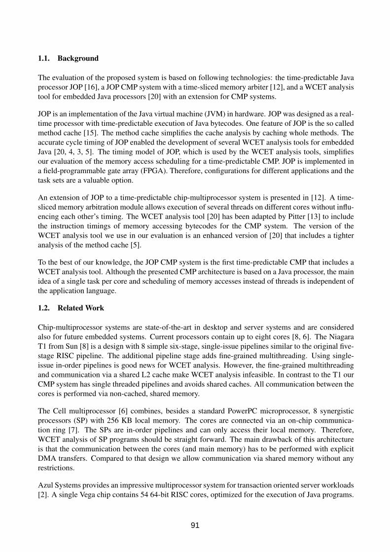
1.1. Background

The evaluation of the proposed system is based on following technologies: the time-predictable Javaprocessor JOP [16], a JOP CMP system with a time-sliced memory arbiter [12], and a WCET analysistool for embedded Java processors [20] with an extension for CMP systems.

JOP is an implementation of the Java virtual machine (JVM) in hardware. JOP was designed as a real-time processor with time-predictable execution of Java bytecodes. One feature of JOP is the so calledmethod cache [15]. The method cache simplifies the cache analysis by caching whole methods. Theaccurate cycle timing of JOP enabled the development of several WCET analysis tools for embeddedJava [20, 4, 3, 5]. The timing model of JOP, which is used by the WCET analysis tools, simplifiesour evaluation of the memory access scheduling for a time-predictable CMP. JOP is implemented ina field-programmable gate array (FPGA). Therefore, configurations for different applications and thetask sets are a valuable option.

An extension of JOP to a time-predictable chip-multiprocessor system is presented in [12]. A time-sliced memory arbitration module allows execution of several threads on different cores without influ-encing each other’s timing. The WCET analysis tool [20] has been adapted by Pitter [13] to includethe instruction timings of memory accessing bytecodes for the CMP system. The version of theWCET analysis tool we use in our evaluation is an enhanced version of [20] that includes a tighteranalysis of the method cache [5].

To the best of our knowledge, the JOP CMP system is the first time-predictable CMP that includes aWCET analysis tool. Although the presented CMP architecture is based on a Java processor, the mainidea of a single task per core and scheduling of memory accesses instead of threads is independent ofthe application language.

1.2. Related Work

Chip-multiprocessor systems are state-of-the-art in desktop and server systems and are consideredalso for future embedded systems. Current processors contain up to eight cores [8, 6]. The NiagaraT1 from Sun [8] is a design with 8 simple six-stage, single-issue pipelines similar to the original five-stage RISC pipeline. The additional pipeline stage adds fine-grained multithreading. Using single-issue in-order pipelines is good news for WCET analysis. However, the fine-grained multithreadingand communication via a shared L2 cache make WCET analysis infeasible. In contrast to the T1 ourCMP system has single threaded pipelines and avoids shared caches. All communication between thecores is performed via non-cached, shared memory.

The Cell multiprocessor [6] combines, besides a standard PowerPC microprocessor, 8 synergisticprocessors (SP) with 256 KB local memory. The cores are connected via an on-chip communica-tion ring [7]. The SPs are in-order pipelines and can only access their local memory. Therefore,WCET analysis of SP programs should be straight forward. The main drawback of this architectureis that the communication between the cores (and main memory) has to be performed with explicitDMA transfers. Compared to that design we allow communication via shared memory without anyrestrictions.

Azul Systems provides an impressive multiprocessor system for transaction oriented server workloads[2]. A single Vega chip contains 54 64-bit RISC cores, optimized for the execution of Java programs.

91

Up to 16 Vega processors can be combined to a cache coherent multiprocessor system resulting in864 processors cores and supporting up to 768 GB of shared memory.

The PRET project is devoted to the development of a time-predictable CMP system [11]. The pro-cessor cores are based on the SPARC V8 instruction set architecture with a six-stage pipeline andsupport chip level multithreading for six threads to eliminate data forwarding and branch prediction.An interesting feature of the PRET architecture is the deadline instruction that stalls the current threaduntil a deadline is reached. This instruction is used to perform time based, instead of lock based, syn-chronization for access to shared data. Besides using processor local scratchpad memories, the sharedmemory it accessed through a so called memory wheel. The memory wheel is a time division, multi-ple access (TDMA) based memory arbiter with equal slot slice. In contrast to the PRET project, weconsider TDMA schedules that can be adapted to the application needs.

The approach, which is closest related to our work, is presented in [1, 14]. The CMP system isintended for tasks according to the simple task model [9]. In this model the task communicationhappens explicitly: input data is read at the begin of the task and output data is written at the end of atask. Furthermore, local cache loading for the cores is performed from a shared main memory. Similarto our approach, a TDMA based memory arbitration is used. The paper deals with optimization of theTDMA schedule to reduce the WCET of the tasks. The design also considers changes of the arbiterschedule during task execution. This implies that all tasks and the cores have to be synchronized withthe memory arbiter, resulting in a cyclic executive model. All tasks, even on different cores, need tofit into a common major cycle.

In contrast to [1, 14], our approach to a TDMA based CMP system allows standard shared memorycommunication without the restrictions of a cyclic executive. Real-time tasks with arbitrary periodsare supported. The approach in [1] uses explicit path enumeration to integrate the TDMA scheduleinto the WCET calculation, which is known to scale poorly. In our system the TDMA scheduleis integrated into an implicit path enumeration based WCET tool [12]. Furthermore, a completeimplementation of the proposed CMP system and the WCET analysis tool are available.

2. WCET Based Memory Access Scheduling

Embedded systems, also called cyber-physical systems, interact with the real world. And the realworld, external to the computer system, is massively parallel. Therefore, embedded systems are goodcandidates for chip-multiprocessing. We argue that the transistors required to implement super-scalararchitectures are better used on complete replication of simple cores for a CMP system [19].

CMP systems share the access bandwidth to the main memory. To build a time-predictable CMPsystem, we need to schedule the access to the main memory in a predictable way. A predictablescheduling can only be time based, where each core receives a fixed time slice. This schedulingscheme is called time division multiple access (TDMA). The execution time of loads, stores, andthe cache miss penalty depend on this schedule. Therefore, the arbiter schedule has to be known todetermine accurate WCET estimates.

Assuming that enough cores are available, we propose a CMP model with a single thread per pro-cessor. In that case thread switching and schedulability analysis for each individual core disappears.Since each processor executes only a single thread, the WCET of that thread can be as long as itsdeadline. When the period of a thread is equal to its deadline, 100% utilization of that core is feasible.

92

For threads that have enough slack time left, we can increase the WCET by decreasing their shareof the bandwidth on the memory bus. Other threads with tighter deadlines can, in turn, use the freedbandwidth and run faster. The consumption of the access bandwidth to main memory is adjustedby the TDMA schedule. The TDMA schedule itself is the input for WCET analysis for all threads.Finding a TDMA schedule, where all tasks meet their deadlines, is thus an iterative optimizationproblem.

It can be argued that the assumption of having fewer tasks than available processing cores is toorestrictive. However, we do not forbid task scheduling on a single core. Our approach is still validwhen more demanding tasks own their core and other tasks share a core under preemptive scheduling.

Two benefits of the single task per core approach have to be emphasized. First, the CPU utilizationon each core can reach 100%, even when the task periods are non-harmonic, and the system is stillanalyzable. Second, the overhead of task dispatching, and the hard to analyze cache thrashing, dis-appears. Both effects lead to tighter WCET bounds and can compensate for idle cycles on the coreswhen the tasks are waiting on their turn to access the memory.

2.1. Memory-Access Scheduling Schemes

Before we look for a particular memory-access schedule for an application running on a multiproces-sor system, we have to decide about the general properties of the scheduling scheme.

• Granularity of the memory access scheduler: one has to decide on scheduling of single mem-ory accesses versus scheduling of longer TDMA slots comprising a larger number of memoryaccesses. Shorter time slices provide the highest flexibility and the most fine-grained control indistributing memory bandwidth among the processors. Longer time slices may improve accesstimes to shared memory if larger blocks from the shared memory have to be transferred at once.

• In case time slices of multiple memory accesses are used, one further has to decide whethertime slices should be of uniform duration or different length. The use of equally sized timeslices provides the simplest solution. Assigning different sizes to the tasks/CPUs makes a betteradaption to application needs possible.

• Single scheduling pattern versus different scheduling patterns. For some applications, the mem-ory access characteristics of the tasks do hardly ever change or the occurrence of particular ac-cess patterns is hard to predict. Such systems may use a single TDMA memory access patternduring their whole operational cycle. Other systems, in contrast, have a number of operationalphases during which the need for memory bandwidth and memory access patterns of the differ-ent tasks/CPUs differ. Such systems benefit from a more flexible memory system that supportsa number of schedules tailored to the needs of the tasks in the different phases of operation.

• Synchronous versus asynchronous operation of memory-access schedules and task execution.One of the most influential decisions on the design of the system is whether the TDMA memoryaccesses and the task execution cycles (i.e., activation times and periods of tasks) are synchro-nized or not. Synchronizing memory access schedules and task operation has the benefit thatmemory access schedules can be optimized to the needs of the tasks during their executioncycle, at the cost of a higher planning effort and a more rigid execution pattern at runtime.Unsynchronized operation is easier to plan, but allows for a less accurate adaption of task andmemory-access behavior.

93

Generate initialarbiter schedule WCET Analysis

WCET Analysis

WCET Analysis Generate arbiterschedule

Arbiterschedule

Task 1

Task 3

Task 2

WCET 1

WCET 3

WCET 2

Systemschedulable

no

Deadlines met? yes

Systemnot

schedulable

Slack left? no

yes

Figure 1. Tool flow for a CMP based real-time system with one task per core and a static arbiter schedule. If thedeadlines are not met, the arbiter schedule is adapted according to the WCETs and deadlines of the tasks. Afterthe update of the arbiter schedule the WCET of all tasks needs to be recalculated.

In the rest of the paper we assume that memory access schedules and task execution are not synchro-nized. Our goal is to find memory access schedules that split the memory bandwidth among the CPUsof the system in such a way that a maximum number of tasks of a given task set meet their timingrequirements. We schedule single memory accesses and, at this time, assume that the same TDMAscheduling sequence is used throughout the whole time of system operation.

2.2. Tool Structure

Figure 1 shows the analysis tool flow for the proposed time-predictable CMP with three tasks. First,an initial arbiter schedule is generated, e.g., one with equal time slices. That schedule and the tasks arethe input of WCET analysis performed for each task individually. If all tasks meet their deadlines withthe resulting WCETs, the system is schedulable. If some tasks do not meet their deadline and othertasks have some slack time available, the arbiter scheduler is adapted accordingly. WCET analysisis repeated, with the new arbiter schedule, until all tasks meet their deadlines or no slack time for anadaption of the arbiter schedule is available. In the latter case no schedule for the system is found.

The TDMA schedule can be adapted along two dimensions. Firstly, the individual slot sizes can bevaried. This variation can be very fine-grained down to single clock cycles. Longer slot sizes aremostly beneficial for burst transfers on a cache load. Secondly, the TDMA round can be adaptedto include several (short) slots for a core within one TDMA round. This leads to lower WCET forindividual memory loads and stores. Which adaption, or if a combination of the two approaches isbeneficial depends on the application characteristic. In the following section both approaches areevaluated for a network application.

94

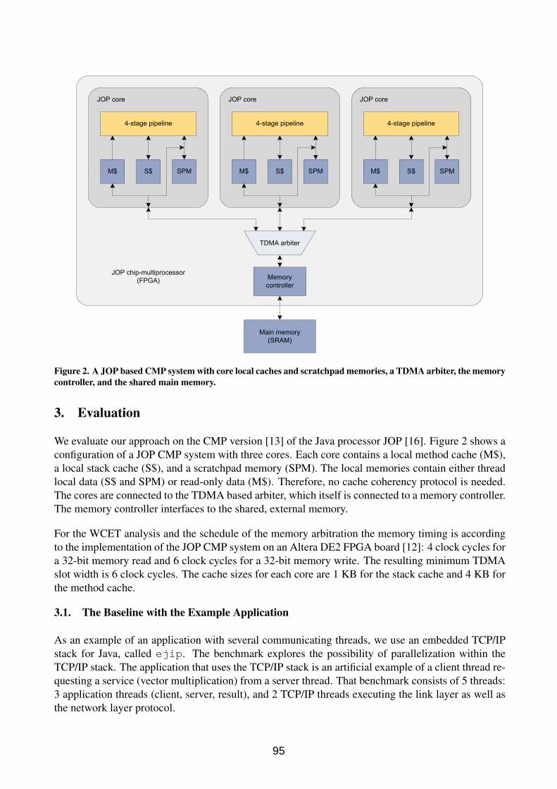
JOP chip-multiprocessor(FPGA)

JOP core

4-stage pipeline

M$ SPMS$

JOP core

4-stage pipeline

M$ SPMS$

JOP core

4-stage pipeline

M$ SPMS$

TDMA arbiter

Memorycontroller

Main memory(SRAM)

Figure 2. A JOP based CMP system with core local caches and scratchpad memories, a TDMA arbiter, the memorycontroller, and the shared main memory.

3. Evaluation

We evaluate our approach on the CMP version [13] of the Java processor JOP [16]. Figure 2 shows aconfiguration of a JOP CMP system with three cores. Each core contains a local method cache (M$),a local stack cache (S$), and a scratchpad memory (SPM). The local memories contain either threadlocal data (S$ and SPM) or read-only data (M$). Therefore, no cache coherency protocol is needed.The cores are connected to the TDMA based arbiter, which itself is connected to a memory controller.The memory controller interfaces to the shared, external memory.

For the WCET analysis and the schedule of the memory arbitration the memory timing is accordingto the implementation of the JOP CMP system on an Altera DE2 FPGA board [12]: 4 clock cycles fora 32-bit memory read and 6 clock cycles for a 32-bit memory write. The resulting minimum TDMAslot width is 6 clock cycles. The cache sizes for each core are 1 KB for the stack cache and 4 KB forthe method cache.

3.1. The Baseline with the Example Application

As an example of an application with several communicating threads, we use an embedded TCP/IPstack for Java, called ejip. The benchmark explores the possibility of parallelization within theTCP/IP stack. The application that uses the TCP/IP stack is an artificial example of a client thread re-questing a service (vector multiplication) from a server thread. That benchmark consists of 5 threads:3 application threads (client, server, result), and 2 TCP/IP threads executing the link layer as well asthe network layer protocol.

95

Function Task Single 5 cores WCET increase

ipLink.run() τ1 1061 2525 2.4resultServer() τ2 1526 3443 2.3request() τ3 8825 23445 2.7macServer() τ4 7004 17104 2.4net.run() τ5 8188 18796 2.3

Sum 26604

Table 1. WCET estimations in clock cycles for a single core and a 5 core system

One bottleneck in the original TCP/IP stack was a global buffer pool. All layers communicated viathis single pool. The single pool is not an issue for a uniprocessor system, however real parallelthreads compete more often for the access to the buffer pool. As a consequence, we have rewrittenthe TCP/IP stack to use dedicated, wait-free, single reader/writer queues [10] for the communicationbetween the layers and the application tasks. The additional benefit of non-blocking communicationis a simplification of the scheduling analysis, as we do not have to take blocking times into account.

For WCET analysis we use a new WCET tool for JOP [5] with an extension for TDMA memoryarbitration [12]. The WCET tool performs the analysis at bytecode instruction level. The executionof bytecodes that access the main memory (e.g., field access, cache load on a method invoke or return)depends on the TDMA schedule. For those bytecodes, the worst-case phasing between the memoryaccesses and the TDMA schedule is considered for the low-level WCET timing.

Table 1 shows the WCET bounds of all 5 tasks obtained by our tool for a single core and a 5 coresystem connected to a TDMA arbiter with a slot size of 6 cycles for each CPU. Due to the memoryaccess scheduling, the WCET increases for each individual task. Although 5 cores compete for thememory access the increase of the WCET is moderate: between a factor of 2.3 and 2.7. As 5 coreslead to an ideal speedup of a factor of 5 and the individual task are slower on that CMP (with respectto the analyzed WCET) by a factor of around 2.5, the net speedup of the 5 core CMP system is arounda factor of 5/2.5 = 2.

To simplify our example we assume that all tasks shall execute at the same period. As this exampleresembles a pipelined algorithm, this assumption is valid. With the default configuration τ3 has thelargest WCET and for a 100 MHz CMP system the minimum period is 23.5 ms. With this periodthe other tasks have a slack time between 4.7 ms and 21 ms. We use that slack time to adapt theTDMA schedule, as shown in Figure 1, to reduce the maximum period for all tasks. We have not yetimplemented the automation of this process, but perform the arbiter schedule generation manually.The resulting WCETs for different arbiter schedules are shown in Table 2, with the equal schedule of6 cycle slots for all cores in the second row for reference. A manual iteration of the arbiter schedulegeneration and WCET analysis loop took a few minutes. The WCET analysis, including data-flowanalysis for loop bounds, takes around 27 s on a standard PC.

3.2. Variation of the Arbiter Schedule

For the first adaption of the arbiter schedule we assumed a quite naive approach: the slot size of thethree longer tasks is doubled to 12 cycles. The result is shown in column Schedule 1 of Table 2. TheWCET for τ4 and τ5 has been reduced, but due to the longer TDMA round (48 cycles instead of 30

96

Task Equal Schedule 1 Schedule 2 Schedule 3 Schedule 4 Schedule 5 Schedule 6

τ1 2525 3605 3605 5045 4325 5285 5525τ2 3443 4865 4865 6761 5813 7077 7393τ3 23445 25313 20211 20201 20473 17955 18681τ4 17104 15284 14860 19468 14276 16756 17376τ5 18796 17856 16432 14832 16204 18924 18364

Table 2. WCET estimations in clock cycles of the application tasks with different arbiter configurations

cycles) the WCET of task τ3 actually increased – an effect into the wrong direction.

For Schedule 2 and Schedule 3 the basic slot size was kept to the minimum of 6 cycles, but differentinter-leavings of the tasks are used: < τ1,τ3,τ4,τ5,τ2,τ3,τ4,τ5 > and < τ3,τ3,τ5, τ5,τ4, τ1,τ3,τ3,τ5,τ5,τ4,τ2 >. For Schedule 3 the repetition of two 6 cycle slots for the same task results effectivelyin a single 12 cycle slot. Both schedules decrease the execution time of task τ3 to 20.2 ms at theexpense of higher execution times of some other tasks.

The following experiments are based on Schedule 2 with variations of the individual slot sizes.We use following notation for the schedule: τi/n is a slot of n cycles for task i. Schedule 4,< τ1/6,τ3/8,τ4/8,τ5/8,τ2/6,τ3/8,τ4/8,τ5/8 > increases the slot size to 8 cycles for all, but tasks τ1and τ2. The resulting minimum period, 20.5 ms, is similar to Schedule 2. To reduce the WCET of τ3we double the slot size for τ3, resulting in Schedule 5, < τ1/6,τ3/16,τ4/8, τ5/8,τ2/6, τ3/16,τ4/8,τ5/8 >, with a minimum period, now determined by task τ5, of 18.9 ms. After several additionaliterations we ended up with Schedule 6, < τ1/6,τ3/16,τ4/8,τ5/10,τ2/6,τ3/16,τ4/8,τ5/10 >, pro-viding the best balanced system for the three demanding tasks and a minimum period of 18.7 ms.Any further increase of individual slot sizes resulted in a higher execution time for τ3, τ4, and τ5.Therefore, not the whole slack time of τ1 and τ2 could be distributed to the other three tasks.

3.3. Discussion

The decrease of the minimum period for all tasks from 23.5 ms to 18.7 ms due to the optimization ofthe memory arbiter schedule is probably not too exciting. However, we started our experiment witha task set that is already quite balanced: three tasks had a similar WCET, and only two tasks had ashorter WCET. The resulting slack time of two tasks can be distributed to the other three tasks.

An interesting question is how the WCET performance scales with a CMP system with a TDMAbased memory arbitration? As we assumed the same period for all tasks we can perform a simplecomparison: when executing the five tasks on a single core the cumulative WCET is the sum of theWCET values as given in Table 1: 26604, resulting in a minimum period of the system of 26.6 ms. Thesame task set on the 5 core CMP system with the optimized arbiter schedule results in a minimumperiod of 18.7 ms. Therefore, the speedup of the WCET due to a 5 core CMP is about 1.4. Thisspeedup is moderate, but it ignores more complex task sets with different periods and the overhead ofpreemptive scheduling on a single core, which is not present in the single task per core setup.

This paper presents a first step towards scheduling of memory accesses instead of tasks. The WCETanalysis considers the arbiter schedule only for memory accesses within a single bytecode. An im-provement of the analysis that considers basic blocks for the interleaving of memory accesses with

97

the TDMA schedule can provide tighter WCET bounds.

With respect to the TDMA schedule we are currently restricted to quite regular schedules. An exten-sion to irregular patterns is straight forward and will enable a finer tuning of the memory bandwidthrequirements.

Furthermore, we have avoided caching of heap data to simplify the predictability of the system. Asa result, each access to heap allocated data has a WCET of a complete TDMA round, which easilyreaches cache miss latencies of current architectures. First ideas on time-predictable data cachingemerge [18]. A small, fully associative data cache will enable analysis of some memory accesses toheap allocated data. Even a low analyzable hit rate of the data cache will improve the WCET of thetasks on the CMP system.

We are confident that the suggested improvements will reduce the WCET of tasks on a CMP systemconsiderable and enable usage of time-predictable CMP systems in hard real-time systems.

4. Conclusion

In this paper, we presented the idea to build chip-multiprocessor real-time systems where each appli-cation task has its own CPU for execution. Therefore, task scheduling is completely avoided. Theremaining shared resource, the main memory and the memory bandwidth, needs to be scheduled. Atime-slicing arbitration of the memory access is the only time-predictable form for CMP systems.When the arbitration schedule is known in advance the worst-case memory access time is known andcan be integrate into WCET analysis.

Furthermore, we have presented an iterative approach to build the schedule for the memory arbiter.Starting from equal sized time slices for each core/task a first WCET estimation for each task iscalculated. Tasks that have a shorter WCET than their deadline can be punished by reducing theirshare of the memory bandwidth. That bandwidth can be used by tasks that do not (yet) meet theirdeadline. The updated arbitration schedule is again used as input for WCET analysis. We havedemonstrated this iterative approach with an example application in the context of a Java processorbased CMP system.

The processor design, the TDMA based CMP design, and the WCET analysis tool are open sourceunder the GNU GPL. The sources are available via git2 and the build instructions can be found in[17].

Acknowledgements

We thank Christof Pitter for the design and implementation of the TDMA arbiter and the integrationinto the WCET tool during his PhD thesis. Furthermore, we are thankful to Benedikt Huber whohas redesigned the WCET analysis tool for JOP during his Master’s thesis. The research leading tothese results has received funding from the European Community’s Seventh Framework Programme[FP7/2007-2013] under grant agreement number 216682 (JEOPARD) and 214373 (Artist Design).

2git clone git://www.soc.tuwien.ac.at/jop.git

98

References

[1] ANDREI, A., ELES, P., PENG, Z., AND ROSEN, J. Predictable implementation of real-timeapplications on multiprocessor systems on chip. In Proceedings of the 21st Intl. Conference onVLSI Design (Jan. 2008), pp. 103–110.

[2] AZUL. Azul compute appliances. Whitepaper, 2009.

[3] BOGHOLM, T., KRAGH-HANSEN, H., OLSEN, P., THOMSEN, B., AND LARSEN, K. G.Model-based schedulability analysis of safety critical hard real-time java programs. In Proceed-ings of the 6th international workshop on Java technologies for real-time and embedded systems(JTRES 2008) (New York, NY, USA, 2008), ACM, pp. 106–114.

[4] HARMON, T. Interactive Worst-case Execution Time Analysis of Hard Real-time Systems. PhDthesis, University of California, Irvine, 2009.

[5] HUBER, B. Worst-case execution time analysis for real-time Java. Master’s thesis, ViennaUniversity of Technology, Austria, 2009.

[6] KAHLE, J. A., DAY, M. N., HOFSTEE, H. P., JOHNS, C. R., MAEURER, T. R., AND SHIPPY,D. J. Introduction to the Cell multiprocessor. j-IBM-JRD 49, 4/5 (2005), 589–604.

[7] KISTLER, M., PERRONE, M., AND PETRINI, F. Cell multiprocessor communication net-work: Built for speed. Micro, IEEE 26 (2006), 10–25.

[8] KONGETIRA, P., AINGARAN, K., AND OLUKOTUN, K. Niagara: A 32-way multithreadedsparc processor. IEEE Micro 25, 2 (2005), 21–29.

[9] KOPETZ, H. Real-Time Systems. Kluwer Academic, Boston, MA, USA, 1997.

[10] LAMPORT, L. Proving the correctness of multiprocess programs. IEEE Transactions on Soft-ware Engineering 3, 2 (1977), 125–143.

[11] LICKLY, B., LIU, I., KIM, S., PATEL, H. D., EDWARDS, S. A., AND LEE, E. A. Predictableprogramming on a precision timed architecture. In Proceedings of the International Conferenceon Compilers, Architecture, and Synthesis for Embedded Systems (CASES 2008) (Atlanta, GA,USA, October 2008), E. R. Altman, Ed., ACM, pp. 137–146.

[12] PITTER, C. Time-predictable memory arbitration for a Java chip-multiprocessor. In Proceed-ings of the 6th international workshop on Java technologies for real-time and embedded systems(JTRES 2008) (Santa Clara, USA, September 2008), ACM Press, pp. 115–122.

[13] PITTER, C. Time-Predictable Java Chip-Multiprocessor. PhD thesis, Vienna University ofTechnology, Austria, 2009.

[14] ROSEN, J., ANDREI, A., ELES, P., AND PENG, Z. Bus access optimization for predictableimplementation of real-time applications on multiprocessor systems-on-chip. In Proceedings ofthe Real-Time Systems Symposium (RTSS 2007) (Dec. 2007), pp. 49–60.

[15] SCHOEBERL, M. A time predictable instruction cache for a Java processor. In On the Move toMeaningful Internet Systems 2004: Workshop on Java Technologies for Real-Time and Embed-ded Systems (JTRES 2004) (Agia Napa, Cyprus, October 2004), vol. 3292 of LNCS, Springer,pp. 371–382.

99

[16] SCHOEBERL, M. A Java processor architecture for embedded real-time systems. Journal ofSystems Architecture 54/1–2 (2008), 265–286.

[17] SCHOEBERL, M. JOP Reference Handbook. No. ISBN 978-1438239699. CreateSpace, 2009.Available at http://www.jopdesign.com/doc/handbook.pdf.

[18] SCHOEBERL, M. Time-predictable cache organization. In Proceedings of the First Interna-tional Workshop on Software Technologies for Future Dependable Distributed Systems (STFSSD2009) (Tokyo, Japan, March 2009), IEEE Computer Society.

[19] SCHOEBERL, M. Time-predictable computer architecture. EURASIP Journal on EmbeddedSystems vol. 2009, Article ID 758480 (2009), 17 pages.

[20] SCHOEBERL, M., AND PEDERSEN, R. WCET analysis for a Java processor. In Proceedingsof the 4th International Workshop on Java Technologies for Real-time and Embedded Systems(JTRES 2006) (New York, NY, USA, 2006), ACM Press, pp. 202–211.

100

SOUND AND EFFICIENT WCET ANALYSISIN THE PRESENCE OF TIMING ANOMALIES1

Jan Reineke2 and Rathijit Sen3

AbstractWorst-Case-Execution-Time (WCET) analysis computes upper bounds on the execution time of a pro-gram on a given hardware platform. Abstractions employed for static timing analysis can lead tonon-determinism that may require the analyzer to evaluate an exponential number of choices evenfor straight-line code. Pruning the search space is potentially unsafe because of “timing anomalies”where local worst-case choices may not lead to the global worst-case scenario. In this paper wepresent an approach towards more efficient WCET analysis that uses precomputed information tosafely discard analysis states.

1. IntroductionEmbedded systems as they occur in application domains such as automotive, aeronautics, and indus-trial automation often have to satisfy hard real-time constraints. Timeliness of reactions is absolutelynecessary. Off-line guarantees on the worst-case execution time of each task have to be derived usingsafe methods.

Static worst-case execution time (WCET) tools employ abstract models of the underlying hardwareplatforms. Such models abstract away from parts of the hardware that do not influence the timingof instructions, like e.g. the values of registers. In addition to the abstraction of data, such modelsfurther abstract components like branch predictors and caches, that have a very large state space.Good abstractions of hardware components can predict their precise concrete behavior most of thetime. However, in general, abstractions introduce non-determinism: whenever the abstract modelcannot determine the value of a condition, it has to consider all possibilities, to cover any possibleconcrete behavior.

Considering all possibilities can make timing analysis very expensive. Even on straight-line code thetiming analyzer might have to consider an exponential number of possibilities in the length of thepath. Often, the different possibilities can be intuitively classified as local worst- or local best-cases:e.g. cache miss vs. cache hit, pipeline stall or not, branch misprediction or not, etc. In such cases, itis tempting to only follow the local worst-case if one is interested in the WCET. Unfortunately, dueto timing anomalies [12, 15] this is not always sound. A timing anomaly is a situation where thelocal worst-case does not entail the global worst-case. For instance, a cache miss—the local worst-case—may result in a shorter execution time, than a cache hit, because of scheduling effects. SeeFigure 1 for an example. Shortening task A leads to a longer overall schedule, because task B cannow block the “more” important task C, which may only run on Resource 2. Analogously, there are

2Universitat des Saarlandes, Saarbrucken, Germany, reineke@cs.uni-saarland.de3University of Wisconsin, Madison, USA, rathijit@cs.wisc.edu1This work has profited from discussions within the ARTIST2 Network of Excellence. It is supported by the German Re-search Foundation (DFG) as part of SFB/TR AVACS and by the European Community’s Seventh Framework ProgrammeFP7/2007-2013 under grant agreement n◦ 216008 (Predator).

101

cases where shortening a task leads to an even greater decrease in the overall schedule. Reineke etal. [15] formally define timing anomalies and give a set of examples for timing anomalies involvingcaches and speculation.

In the presence of timing anomalies it is unsound toA

A

Resource 1

Resource 2

Resource 1

Resource 2

C

B C

B

D E

D E

Figure 1. Scheduling Anomaly.

simply discard non local-worst-cases. We assumethat most if not all modern processors exhibit tim-ing anomalies and that there is little hope to con-struct processors with good performance that do notexhibit them. To obtain an efficient timing analysis,we would still like to discard non-local-worst-casestates, yet in a sound way. Our idea is to performa precomputation on the abstract model of the hard-

ware, that is used for timing analysis. The precomputation computes for each pair of analysis states abound on the future difference in timing between the two states. This precomputation might be veryexpensive, but it only has to be done once for a particular abstract hardware model. Timing analysesusing this hardware model can then safely discard analysis states based on the precomputed differ-ences, even in the presence of timing anomalies. Assuming that timing anomalies occur seldomly andcan be excluded using the precomputation most of the time, the proposed analysis will be much moreefficient than previous exhaustive methods.

2. Related WorkGraham [7] shows that a greedy scheduler can produce a longer schedule, if provided with shortertasks, fewer dependencies, more processors, etc. Graham also gives bounds on these effects, whichare known as scheduling anomalies today.

Lundqvist & Stenstrom first introduced timing anomalies in the sense relevant for timing analysis. In[12] they give an example of a cache miss resulting in a shorter execution time than a cache hit. Atiming anomaly is characterized as a situation where a positive (negative) change of the latency of thefirst instruction results in a global decrease (increase) of the execution time of a sequence of instruc-tions. Situations where the local effect is even accelerated are also considered timing anomalies, i.e.the global increase (decrease) of the execution time is greater than the local change.

In his PhD thesis [3] and a paper with Jonsson [4], Engblom also discusses timing anomalies. Hetranslates the notion of timing anomalies of the Lundqvist/Stenstrom paper [12] to his model byassuming that single pipeline stages take longer, in contrast to whole instructions. Both Lundqvistand Engblom claim that, in processors that contain in-order resources only, no timing anomalies canoccur. This is not always true unfortunately, as corrected in Lundqvist’s thesis [11]. Schneider [17]and Wenzel et al. [21] note that if there exist several resources that have overlapping, but unequalcapabilities, timing anomalies can also occur.

Reineke et al. [15] provide the first formal definition of timing anomalies. The definition of timinganomalies in this paper is a slight relaxation of that of [15]. In recent work, Kirner et al. [9] introducethe notion of parallel timing anomalies. Such anomalies arise if a WCET analysis is split into theanalysis of several hardware components that operate in parallel. Depending on how the analysisresults are combined the resulting WCET estimate may be unsafe. The authors identify conditionsthat guarantee the safety of two combination methods. This work is orthogonal to ours.

102

3. Static WCET Analysis FrameworkOver the last several years, a more or less standard architecture for static timing-analysis tools hasemerged [8, 19, 5]. Figure 2 gives a general view on this architecture. One can distinguish threemajor building blocks:

1. Control-flow reconstruction and static analyses for control and data flow.

2. Micro-architectural analysis, which computes upper and lower bounds on execution times ofbasic blocks.

3. Global bound analysis, which computes upper and lower bounds for the whole program.

Micro-architectural analysis [6, 11, 3, 20, 10, 16] determines

BinaryExecutable

CFG Re-construction

Control-flowGraph

Loop BoundAnalysis

ValueAnalysis

Control-flowAnalysis

AnnotatedCFG

Basic BlockTiming Info

Micro-architectural

Analysis

GlobalBound

Analysis

Legend:

Data

Phase

Figure 2. Main components of a timing-analysis framework and their interac-tion.

bounds on the execution time of basic blocks, taking into ac-count the processor’s pipeline, caches, and speculation con-cepts. Static cache analyses determine safe approximations tothe contents of caches at each program point. Pipeline analysisanalyzes how instructions pass through the pipeline accountingfor occupancy of shared resources like queues, functional units,etc. Ignoring these average-case-enhancing features would re-sult in very imprecise bounds.

In this paper, we consider micro-architectural analyses that arebased on abstractions of the concrete hardware and that prop-agate abstract states through the control-flow-graph [3, 20, 6].In such analyses, the micro-architectural analysis is the mostexpensive part of the WCET analysis. Due to the introductionof non-determinism by abstraction and the possibility of tim-ing anomalies it is necessary to consider very many cases. Forcomplex architectures, this may yield hundreds of millions ofanalysis states, and may thus be very memory and time intensive.

In the following, we will describe a simple, formal model of such a micro-architectural analysis.Later, we will describe how this model can be extended to enable more efficient analyses.

3.1. A formal model of micro-architectural analysis

Micro-architectural analysis determines bounds on the execution times of basic blocks. Using anabstract model of the hardware, it “simulates” the possible behavior of the hardware in each cycle.Due to uncertainty about the concrete state of the hardware or about its inputs, abstract models are—unlike usual cycle-accurate simulators—non-deterministic. Therefore, an abstract state may haveseveral possible successor states.

Cycle semantics. Let State be the set of states of the abstract hardware model, and let Prog bethe set of programs that can be executed on the hardware. Then the cycle semantics can be formallymodeled by the following function:

cycle : State× Prog → P(State).

103

IDIF MEMEX WB

IDIF MEMEX WB

IDIF MEMEX WB

IDIF MEMEX WB

0 1 2 3 4 5 6 7 8 9Cycles

Inst

ruct

ions

I1I2I3I4I5 IF

I1 I2 I3 I4 I5 ...

ID EX MEM WB

10

Association of cycles to instructions

Figure 3. Pipelined execution of several instructions and association of instructions with execution cycles (bottom).

It takes an abstract state and a program and computes the set of possible successor states. Such anabstract hardware model can be proved correct by showing that it is an abstract interpretation [2] ofthe concrete hardware model. To bound the execution time of a basic block, one needs to associateexecution cycles with instructions in the program. In pipelined processors several instructions areexecuted simultaneously, see Figure 3. There is no canonical association of execution cycles to in-structions. One of several possibilities is to associate a cycle with the last instruction that was fetched.This is exemplified in the lower part of Figure 3.

Instruction semantics. Based on such a connection between execution cycles and instructions,one can lift the cycle semantics to an instruction semantics. This instruction semantics takes anabstract hardware state and an instruction that is to be fetched and computes the set of possible abstracthardware states until the next instruction can be fetched. Each of the resulting abstract hardware statesis associated with the number of cycles to reach this state:

execI : State× I → P(State× N).

For a formalization of the connection of the two semantics, see [20]. As an example of the twosemantics in the analysis of the execution of a basic block, see Figure 4.

Instruction semantics can be easily lifted to the execution of basic blocks, which are simply sequencesof instructions ∈ I∗:

execBB : State× I∗ → P(State× N)

execBB(s, ε) := {(s, 0)}execBB(s, ι0 . . . ιn) := {(s′′, t′ + t′′) | (s′, t′) ∈ execI(s, ι0) ∧

(s′′, t′′) ∈ execBB(s′, ι1 . . . ιn)}As a shortcut, we will also write s t′−→ι s′ for (s′, t′) ∈ execI(s, ι) and similarly s

t′−−−→ι0...ιns′ for

(s′, t′) ∈ execBB(s, ι0 . . . ιn).

Bounds on the execution times of basic blocks. Given an instruction semantics on a finite set ofstates State, one can compute bounds on the execution times of the basic blocks of a program. To thatend, one can compute the set of abstract states that might reach the start of each basic block througha fixed-point iteration. For each of the states that might reach a basic block, the instruction semanticscan then be used to compute the maximum execution time of the block starting in that state:

max(s, ι0 . . . ιn) := max{t | s t−−−→ι0...ιns′}. (1)

104

Basic

Blo

ck

InstructionInstruction

Cycle semantics: Instruction semantics:

3 3 3 2

1 2 2 22 2 2

Figure 4. Cycle semantics and instruction semantics of a basic block.

Finally, the maximum of these times for each state reaching a basic block is an upper bound on theexecution time of that basic block in the given program. Analogously to the computation of upperbounds one can also compute lower bounds on the execution time of a basic block by the min function:

min(s, ι0 . . . ιn) := min{t | s t−−−→ι0...ιns′}. (2)

4. Timing Anomalies, Domino Effects, and How to Safely Discard StatesThe approach described in the previous section can be very expensive. Due to non-determinismintroduced by abstraction, the set of states to be considered can be extremely large. It is thereforetempting to discard states that are non local-worst-case, e.g., states resulting from a cache hit, if botha cache hit and a cache miss may happen.

4.1. Timing anomalies

Unfortunately, due to so-called timing anomalies [12] this is not always sound. The following is adefinition of timing anomalies that is slightly relaxed compared with that of [15].

Definition 1 (Timing anomaly). An instruction semantics has a timing anomaly if there exists asequence of instructions ι0ι1 . . . ιn ∈ I∗, and an abstract state s ∈ State, such that

• there are states s1, s2 ∈ State, with s t1−→ι0 s1 and s t2−→ι0 s2, and t1 < t2, such that

• t1 + max(s1, ι1 . . . ιn) > t2 + max(s2, ι1 . . . ιn).

In an instruction semantics with timing anomalies it is unsound to discard a non-local-worst-casestate (like s1 in the definition). The execution of non-local-worst-case states may be so much slowerthan the execution of local-worst-case states, that the non-local-worst-case state yields the globalworst-case timing. Experience shows that reasonable abstract instruction semantics for most modernprocessors exhibit timing anomalies.

4.2. How to safely discard analysis states

Our approach is to precompute a function ∆ : State × State → N∞, where N∞ = N ∪ {∞}, thatbounds the maximal difference in worst-case timing between the two states on any possible instructionsequence. Sometimes the difference in timing between two states cannot be bounded by any constant.That is why we augment N with∞. The order of natural numbers is lifted to N∞ by adding∞ ≥ nfor all n ∈ N∞.

105

Definition 2 (Valid ∆). A ∆ function is valid, if for all pairs of states s1, s2 ∈ State and for allinstruction sequences ι0 . . . ιn ∈ I∗:

∆(s1, s2) ≥ max(s1, ι0 . . . ιn)−max(s2, ι0 . . . ιn).

Given such a ∆ function it is possible to safely discard analysis states. If the analysis encounters twostates s1 and s2 with execution times t1 and t2, respectively, it may discard s2 if t1 − t2 ≥ ∆(s2, s1)and s1 if t2 − t1 ≥ ∆(s1, s2). In these cases, the discarded state can never overtake the other state.So ∆ can be used to locally exclude the occurrence of a timing anomaly. It is expected that this isoften the case, as timing anomalies are not the common case. This optimization does not influencethe precision of the analysis.

Even if t1 − t2 < ∆(s2, s1), one can safely discard s2, by adding the penalty ∆(s2, s1) − (t1 − t2)to t1. For the resulting t′1 = t1 + ∆(s2, s1) − (t1 − t2), it holds that t′1 − t2 ≥ ∆(s2, s1). In contrastto the first optimization, this of course comes at the price of decreased precision. This optimizationoffers a way of trading precision for efficiency.

4.3. Domino effects

Unfortunately, the difference in timing between two states cannot always be bounded by a constant.This situation is known as a domino effect1.

Definition 3 (Domino effect). An instruction semantics has a domino effect if there are two statess1, s2 ∈ State, such that for each ∆ ∈ N there is a sequence of instructions ι0 . . . ιn ∈ I∗, such that

max(s1, ι0 . . . ιn)−max(s2, ι0 . . . ιn) ≥ ∆.

In other words, there are two states whose timing may arbitrarily diverge. Such effects are known toexist in pipelines [17] and caches [1, 14]. If such domino effects exist for many pairs of states, valid∆ functions will often have value ∞. In that case, the ∆ function is rather useless; it can rarely beused to discard states.

Although the difference in execution times may not be bounded by a constant, the ratio between thetwo execution times is always bounded, i.e., max(s1,ι0...ιn)

max(s2,ι0...ιn)< ρ for some constant ρ. An alternative to

computing ∆ functions is to compute two functions ρ : State×State→ Q and δ : State×State→Q that together bound the maximal difference between the two states in the following way:

Definition 4 (Valid ρ and δ functions). A pair of functions ρ and δ is valid, if for all pairs of statess1, s2 ∈ State and instruction sequences ι0 . . . ιn ∈ I∗ :

max(s1, ι0 . . . ιn) ≤ ρ(s1, s2) ·max(s2, ι0 . . . ιn) + δ(s1, s2).

If there are no domino effects, there are valid ρ and δ functions in which ρ is 1 everywhere. In thatcase, δ is valid in the sense of Definition 2. Otherwise, ρ and δ can still be used to safely discardstates: Say the analysis wants to discard a state s1 with execution time t1, but keep another state s2

with execution time t2, s.t. ρ(s1, s2) = 1.05 and δ(s1, s2) = 5. Then, the analysis could discard s1,but remember to multiply the future execution time of s2 by 1.05. Also, similarly to the case of ∆functions, if t2 − t1 < 5, it would have to add 5− (t2 − t1) to t2.

1Domino effects are also known as unbounded timing effects [11].

106

5. Computation of Valid ∆ FunctionsGiven an instruction semantics, how to compute a valid ∆ function? Of course, one cannot sim-ply enumerate all sequences of instructions. However, it is possible to define a system of recursiveconstraints whose solutions are valid ∆ functions. These recursive equations correspond to the exe-cution of no instruction at all or to the execution of a single instruction. Therefore, a finite number ofconstraints will suffice.

As ∆ needs to bound the difference in timing for all instruction sequences, it must do so in particularfor the empty sequence. This implies the constraints

∆(s1, s2) ≥ 0 (3)

for all s1, s2 ∈ State. Longer sequences can be covered by the recursive constraints

∆(s1, s2) ≥ t′1 − t′2 + ∆(s′1, s′2) (4)

for all s1, s2, s′1, s′2 ∈ State such that s1

t′1−→ι s′1 ∧ s2

t′2−→ι s′2 for some ι.

Theorem 1. Any solution ∆ to this set of constraints is a valid ∆ function.

Proof. A ∆ function that satisfies the above constraints actually fulfills a stronger condition thanvalidity. The constraints guarantee that ∆(s1, s2) ≥ max(s1, ι0 . . . ιn) − min(s2, ι0 . . . ιn) for alls1, s2 ∈ State and ι0 . . . ιn ∈ I∗. Proof by induction over the length of the sequence ι0 . . . ιn:

Base case: We have to show that ∆(s1, s2) ≥ max(s1, ε)−min(s2, ε). Since max(s1, ε)−min(s2, ε) = 0,this is trivially fulfilled by satisfaction of the ∆(s1, s2) ≥ 0 constraints.

Inductive step: We have to show that ∆(s1, s2) ≥ max(s1, ι0 . . . ιn+1) − min(s2, ι0 . . . ιn+1) giventhat ∆(s1, s2) ≥ max(s1, ι1 . . . ιn+1)−min(s2, ι1 . . . ιn+1). The recursive constraints guarantee that

∆(s1, s2) ≥ max{t′1 − t′2 + ∆(s′1, s′2) | s1

t′1−→ι0 s′1 ∧ s2

t′2−→ι0 s′2}.

Plugging the induction hypothesis (I.H.) for ∆(s′1, s′2) into this yields

∆(s1, s2)I.H.≥ max{t′1 − t′2 + max(s′1, ι1 . . . ιn+1)−min(s′2, ι1 . . . ιn+1) | s1

t′1−→ι0 s′1 ∧ s2

t′2−→ι0 s′2}Eq. 1,2

= max{t′1 − t′2 + t′′1 − t′′2 | s1

t′1−→ι0 s′1 ∧ s′1t′′1−−−−−→ι1...ιn+1

s′′1 ∧ s2

t′2−→ι0 s′2 ∧ s′2t′′2−−−−−→ι1...ιn+1

s′′2}

= max{t′1 + t′′1 | s1

t′1−→ι0 s′1 ∧ s′1t′′1−−−−−→ι1...ιn+1

s′′1} −min{t′2 + t′′2 | s2

t′2−→ι0 s′2 ∧ s′2t′′2−−−−−→ι1...ιn+1

s′′2}Eq. 1,2

= max(s1, ι0 . . . ιn+1)−min(s2, ι0 . . . ιn+1)

The lower the function value of ∆, the more states can be discarded using ∆. We are thereforecomputing the least solution to the set of constraints.

Our constraints fall into the class of difference constraints. The least solution of a system of differenceconstraints can be found by solving a shortest path problem [13]. To compute this efficiently, one canuse Tarjan’s algorithm of subtree disassembly and FIFO selection rule [18]. Negative cycles in the

107

constraint graph correspond to domino effects. Tarjan’s algorithm allows for an efficient detectionand elimination of these cycles. The least solution for pairs of states on these cycles is∞.

We have also implemented a solution to compute valid ρ and δ functions, which allows to boundthe effect of domino effects. However, due to space constraints, we cannot present the theoreticalbackground and the results of these computations here.

6. Case StudyWe used the analysis technique described above on a processor model that includes a decoupledfetch pipeline, multi-cycle functional units and variable memory access latencies. Figure 5 showsa diagrammatic representation of this model. E0 through Ek represent functional units that executeinstructions. A particular instruction may be scheduled to be executed on any one of a subset ofthe available functional units. The L/S unit is for load-store instructions only. Our model currentlydoes not consider delays due to reorder-buffer unavailability or bus contention cycles. However, stallsdue to data dependencies, functional unit occupancy, and limited fetch buffer space are considered.Speculative execution is not modeled.

Specifications of instances of this model are used

Figure 5. Processor Architecture

as inputs to our analysis engine that computes the∆ function as described in Section 5. A simple ar-chitecture description language is used to describethe processors. The size of the state space is re-duced by exploiting symmetries in the specifica-tion. For example, instructions are classified intotypes according to their execution latencies. Theanalyzer first builds a transition system correspond-ing to this specification. Each state in the transi-tion system comprises of the states of the functionalunits, fetch buffers, and fetch and data accesses intransit. The edge between any two adjacent states,S1 and S2 in this transition system is annotated withthe pair (t,I) that indicates a transition from stateS1 to S2 after t cycles due to execution of instruc-tion I. Once we have built this transition system

we can construct the constraint system described in the previous section in a straightforward way.

Figure 6 shows part of the transition system for a processor with a domino effect. In this processor,functional unit E0 is optimized for instruction type I1 whereas E1 is optimized for I2. I1 needs 2cycles to execute on E0, but 4 cycles on E1. The timing requirements for I2 are opposite. There are2 fetch buffers that are drained in order and Icache hit time is 1 cycle. In the figure, Ij:m indicatesthat instruction type Ij is in its mth cycle of execution on that functional unit. A shaded functionalunit indicates a new instruction dispatch (m=1) that cycle. The figure shows that the timing differencebetween paths starting from states S0 and S4 is 1 clock cycle per loop. The timing difference is thusunbounded on the instruction sequence (I1.I2)∗. It is useful to use the cycle ratio (4/3) in this case.

The transition system for a simple processor example with 2 instruction types, 2 functional units,execution times ranging from 2 to 6 cycles, 4 fetch buffers and no domino effects had 555 states andgenerated 97340 constraints. The ∆ function ranged from 0 through 7 with 0s forming 88.1% of

108

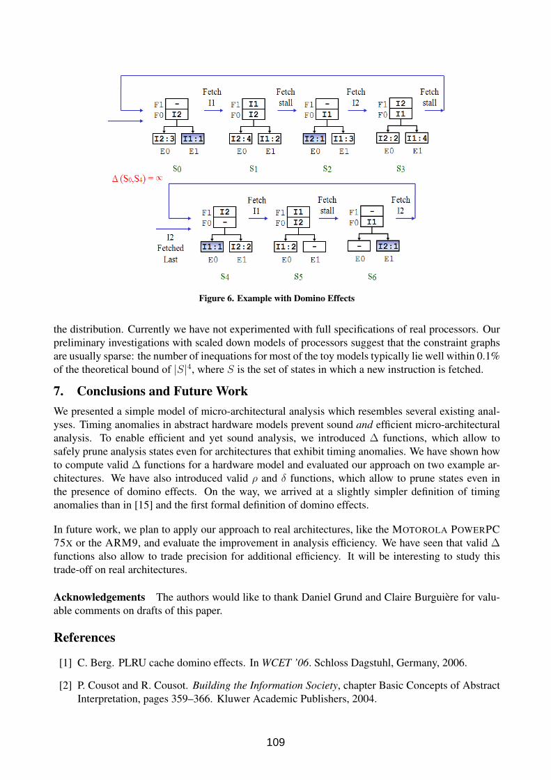
Figure 6. Example with Domino Effects

the distribution. Currently we have not experimented with full specifications of real processors. Ourpreliminary investigations with scaled down models of processors suggest that the constraint graphsare usually sparse: the number of inequations for most of the toy models typically lie well within 0.1%of the theoretical bound of |S|4, where S is the set of states in which a new instruction is fetched.

7. Conclusions and Future WorkWe presented a simple model of micro-architectural analysis which resembles several existing anal-yses. Timing anomalies in abstract hardware models prevent sound and efficient micro-architecturalanalysis. To enable efficient and yet sound analysis, we introduced ∆ functions, which allow tosafely prune analysis states even for architectures that exhibit timing anomalies. We have shown howto compute valid ∆ functions for a hardware model and evaluated our approach on two example ar-chitectures. We have also introduced valid ρ and δ functions, which allow to prune states even inthe presence of domino effects. On the way, we arrived at a slightly simpler definition of timinganomalies than in [15] and the first formal definition of domino effects.

In future work, we plan to apply our approach to real architectures, like the MOTOROLA POWERPC75X or the ARM9, and evaluate the improvement in analysis efficiency. We have seen that valid ∆functions also allow to trade precision for additional efficiency. It will be interesting to study thistrade-off on real architectures.

Acknowledgements The authors would like to thank Daniel Grund and Claire Burguiere for valu-able comments on drafts of this paper.

References

[1] C. Berg. PLRU cache domino effects. In WCET ’06. Schloss Dagstuhl, Germany, 2006.

[2] P. Cousot and R. Cousot. Building the Information Society, chapter Basic Concepts of AbstractInterpretation, pages 359–366. Kluwer Academic Publishers, 2004.

109

[3] J. Engblom. Processor Pipelines and Static Worst-Case Execution Time Analysis. PhD thesis,Uppsala University, 2002.

[4] J. Engblom and B. Jonsson. Processor pipelines and their properties for static WCET analysis.In EMSOFT’02, pages 334–348, London, UK, 2002. Springer-Verlag.

[5] A. Ermedahl. A Modular Tool Architecture for Worst-Case Execution Time Analysis. PhD thesis,Uppsala University, 2003.

[6] C. Ferdinand and R. Wilhelm. Efficient and precise cache behavior prediction for real-timesystems. Real-Time Systems, 17(2-3):131–181, 1999.

[7] R. L. Graham. Bounds on multiprocessing timing anomalies. SIAM Journal of Applied Mathe-matics, 17(2):416–429, 1969.

[8] C. A. Healy, D. B. Whalley, and M. G. Harmon. Integrating the timing analysis of pipeliningand instruction caching. In RTSS’95, pages 288–297, Dec. 1995.

[9] R. Kirner, A. Kadlec, and P. Puschner. Precise worst-case execution time analysis for processorswith timing anomalies. In ECRTS’09, July 2009.

[10] X. Li, A. Roychoudhury, and T. Mitra. Modeling out-of-order processors for WCET analysis.Real-Time Systems, 34(3):195–227, November 2006.

[11] T. Lundqvist. A WCET Analysis Method for Pipelined Microprocessors with Cache Memories.PhD thesis, Chalmers University of Technology, Sweden, June 2002.

[12] T. Lundqvist and P. Stenstrom. Timing anomalies in dynamically scheduled microprocessors.In RTSS’99, Washington, DC, USA, 1999. IEEE Computer Society.

[13] V. R. Pratt. Two easy theories whose combination is hard. Technical report, MassachusettsInstitute of Technology, 1977.

[14] J. Reineke. Caches in WCET Analysis. PhD thesis, Universitat des Saarlandes, Saarbrucken,Germany, November 2008.

[15] J. Reineke, B. Wachter, S. Thesing, R. Wilhelm, I. Polian, J. Eisinger, and B. Becker. A definitionand classification of timing anomalies. In WCET’06. Schloss Dagstuhl, Germany, July 2006.

[16] C. Rochange and P. Sainrat. A context-parameterized model for static analysis of executiontimes. Trans. on High-Performance Embedded Arch. and Compilers, 2(3):109–128, 2007.

[17] J. Schneider. Combined Schedulability and WCET Analysis for Real-Time Operating Systems.PhD thesis, Saarland University, Germany, Saarbrucken, Germany, December 2002.

[18] R. E. Tarjan. Shortest paths. Technical report, AT&T Bell Laboratories, Murray Hill, NJ, 1981.

[19] H. Theiling, C. Ferdinand, and R. Wilhelm. Fast and precise WCET prediction by separatedcache and path analyses. Real-Time Systems, 18(2/3):157–179, May 2000.

[20] S. Thesing. Safe and Precise WCET Determination by Abstract Interpretation of Pipeline Mod-els. PhD thesis, Saarland University, Saarbrucken, Germany, 2004.

[21] I. Wenzel, R. Kirner, P. Puschner, and B. Rieder. Principles of timing anomalies in superscalarprocessors. In Proc. 5th International Conference on Quality Software, Sep. 2005.

110

A GENERIC FRAMEWORK FOR BLACKBOXCOMPONENTS IN WCET COMPUTATION

C. Ballabriga, H. Cassé, M. De Michiel1

AbstractValidation of embedded hard real-time systems requires the computation of the Worst Case ExecutionTime (WCET). Although these systems make more and more use of Components Off The Shelf (COTS),the current WCET computation methods are usually applied to whole programs: these analysis meth-ods require access to the whole system code, that is incompatible with the use of COTS. In this paper,after discussing the specific cases of the loop bounds estimation and the instruction cache analysis,we show in a generic way how static analysis involved in WCET computation can be pre-computedon COTS in order to obtain component partial results. These partial results can be distributed withthe COTS, in order to compute the WCET in the context of a full application. We describe also theinformation items to include in the partial result, and we propose an XML exchange format to repre-sent these data. Additionally, we show that the partial analysis enables us to reduce the analysis timewhile introducing very little pessimism.

1. Introduction

Critical hard real-time systems are composed of tasks which must imperatively finish before theirdeadline. To guarantee this, a task scheduling analysis, that requires the knowledge of each taskWCET, is performed. To compute the WCET, we must take into account (1) the control flow of thetask (flow analysis) and (2) the host hardware (timing analysis). The current WCET computationmethods are designed to be used on a whole program. However, there is some drawbacks to thisapproach. First, the analyses used for WCET computation usually run in exponential time with respectto the program size. Second, when the program to analyze depends on external components (e.g.COTS or libraries) whose sources are not available, the lack of information about the componentsprevents the WCET computation if information from the user is requested.

This paper focuses on the last problem, but it is shown that, as a side-effect, the computation time isalso decreased. This article presents a generic method to partially analyze a black-box component,producing a component partial result that may be instantiated at each component call point to produceactual analysis results. We also define the information items that must be included in the componentpartial result, and propose an XML exchange file format.

As WCET computation involves a lot of analyses, the first section presents two of them as examples,the instruction cache analysis and the loop bound estimation, and show how to adapt them to be ableto do partial analysis. Then, in the next section, we generalize our approach based on the previouslydescribed examples. We present our implementation (XML exchange format definition, and exper-imental results with OTAWA) in the third section and, after presenting related works in section 5,

1IRIT, Université de Toulouse, CNRS - UPS - INP - UT1 - UTM, 118 rte de Narbonne, 31062 Toulouse cedex 9,email: {ballabri,casse}@irit.fr

111

we conclude in the last section.

2. Component analysis

To compute the WCET of a program, one must previously perform a lot of analyses, some relatedto the flow control analysis (infeasible paths detection, loop bounds evaluation, etc), other related tothe architecture effects analysis (cache analysis, branch predictor analysis, etc). The actual WCETcomputation can be done in several ways, but a widely used approach is IPET [14] (Implicit PathEnumeration Technique). This technique assigns a variable to each Basic Block (BB) and edge, repre-senting the number of executions on the path producing the WCET and builds a linear constraint sys-tem with these variables to represent the program structure and the flow facts (such as loop bounds).The WCET is then the maximization of an objective function depending on these variables and on theindividual execution time of each BB computed by an ILP (Integer Linear Programming) solver.

To explain the general principles of component analysis, we study a simple scenario where a programmain() is calling a function callee() in a component. Well known analyses involved in WCETare used: the instruction cache behavior analysis and the loop bounds analysis. For each one, we showhow to partially analyse the callee() function to produce a partial result PRcallee. Then we showhow to analyse the program main() while composing informations from PRcallee (but without anyaccess to the callee() code), to obtain analysis results for the whole program.

2.1. Instruction Cache Analysis

The partial cache analysis method presented in this section is based on the whole-program instructioncache1 analysis presented by [12, 1] and improved in [2], which computes, by static analysis, a cat-egory describing a particular cache behavior for each instruction. The instructions whose executionalways result in a cache hit (resp. miss) are categorized as Always Hit (AH) (resp. Always Miss -AM). A third category, Persistent (PS), exists for the instructions whose first reference may result in acache miss, while the subsequent references result in cache hits. Other cases are set to Not Classified(NC). From these categories, new ILP constraints are added to the ILP system.

The categories are computed by abstract interpretation [8, 9] on a Control Flow Graph (CFG), com-posed of BB. Abstract Cache States (ACS) are computed before and after each BB which are in turnused to compute the categories. Three different analyses are done, each one using its own kind ofACS: the May, the Must, and Persistence analyses. While the May (resp. Must) analyses computesthe cache blocks that may (resp. must) be in the cache, the Persistence finds the persistent blocks.

As previously stated in [4], three issues exist when dealing with partial instruction cache analysis.First, when executed, the callee() function ages and/or evicts cache blocks from the main programand so, it affects the categorization of the main program blocks. This is modeled by a cache transferfunction (based on previous works by A. Rakib et al. in [18]) for each cache analysis. This transferfunction is defined by ACSafter

type = transfer(ACSbeforetype ) (where type is one of may, must, or pers).

In other words, it gives, for each cache analysis, the ACS after the function call based on the ACSbefore. Second, the callee() function contains blocks that need to be categorized. Unfortunately,the categorization of these blocks is not constant, but depends on the ACS at the function calling site.

1In this paper, we suppose that we have a set-associative instruction cache with Least Recently Used (LRU) replacementpolicy.

112

So we have introduced in [4] a summary function (only one is necessary to handle the three analyses)that is defined by cat = summary(ACSbefore

must , ACSbeforemay , ACSbefore

pers ), where cat is a ConditionalCategory (CC), i.e. a function such that cat : Block → {AH |AM |PS |NC }. In other words,it takes the various ACS before the call, and returns a category for each BB of callee().

The last problem is that, when doing the partial analysis on callee(), the component base addressis not known while it dictates which cache lines are affected by ageing, and which blocks are loaded.To take this into account, we force the alignment of cache blocks boundaries on callee() to bethe same at partial analysis time and at instantiation time by enforcing the actual base address to bealigned on cache block size. Then, the matching between line results at partial analysis time andinstantiation time is just a matter of shift and roll on the whole set of lines. This constraint may beeasily achieved with most linkers.

Once we have the callee() partial result, the composition with the main program is done in twosteps (illustrated in figure 1), without any further access to the callee() source code or executable:

1. We perform the instruction cache analysis on the main program in the same way as we wouldhave done on a traditional (monolithic) analysis, except that we model the calls to the callee()function by the transfer function. At the end of this step, we obtain the ACS before and aftereach BB of main().

2. Next, as we know the ACS values for main(), we have the ACS at the calling site ofcallee() and, therefore we can apply the summary function to obtain the categorizationof callee() blocks.

At the end, we have got the categorization for all BB of the program (including component BB).

2.2. Loop Bound Analysis

The loop bound partial analysis presented in this paper is based on works of [10]. It tries to estimatesthe max and total iteration count for each loop in the program (the max is the maximum number ofiterations for one entry into the loop, while the total is the total number of iterations of the loop duringthe execution of the outermost loop). The loop bound estimation is performed in three steps:

1. First, a context tree representing the program is built (a context tree is a tree where nodesare loops or function calls, and where children nodes are inner loops or function calls), andeach loop is represented by a normal form. This normal form enables us (if possible) to get anexpression representing the maximum iteration number of the loop, parametrized by the contextof the loop. The computation uses abstract interpretation, in which the domain is an AbstractStore (AS) that maps each variable in the program to a symbolic expression describing its value.

2. The second step performs a bottom-up traversal of the context tree and instantiates each parame-trized expression of max and total (computed in first step) to get absolute, context-dependantexpressions for each loop.

3. Although the second step computes max and total expressions for each loops, it remains com-plex expressions that are evaluated in this last step to get a numerical value. Finally, a treeannotated with the results for each loop is returned by the analysis.

113

To perform partial loop bound analysis, we need (1) to determine the effect of the call to callee()on the main program (side effects, modified global variables, reference-passed arguments), and (2) tosupply parametrized loop bound expressions depending on the calling context.

In fact, the analysis proposed in [10] is well suited to perform partial analysis. For the sub-problem(1), the Abstract Stores represents values of the program variables as symbolic expressions, that is,they support free variables representing data provided in the caller context. Therefore, performing thetransfer function is just replacing the context variables by their actual values in the Abstract Store atthe exit of the component. This allows us to satisfy the sub-problem (1), but it can be refined: to avoidwasting memory and computation time, we can trim the component Abstract Store by eliminating thevariables that cannot have an effect on the main program. Only the remainder is part of the partialresult of callee().

To handle the sub-problem (2), we have to analyze the callee() function on its own (as if it wasthe main entry point). We need to perform the analysis up to (and including) step (2) that provides thesymbolic expressions of the max and total for all loops in callee(). Then, it is easy to apply a con-text Abstract Store to this symbolic values at composition time by replacing free variables by theiractual values. These symbolic expressions are stored in the partial result computed for callee().

To sum up: the partial result for callee() contains (1) the (trimmed) component Abstract Storeplaying role of the transfer function and (2) the symbolic expressions of the max and total, used asa summary of the component. Likewise to the cache partial analysis, the obtained partial results arecomposed in two steps:

1. First, loop bound analysis is performed on the main program, while modeling callee() bythe Abstract Store. This enables us to know the max and total bounds for the loops in main().

2. Second, as we have got the calling context of callee(), we can apply it to the symbolicexpressions of its loop bounds.

We can see a lot of similarities between the partial cache analysis and the partial loop bound analysisapproaches. The next section proposes a generalization to other analyses.

3. Generic Principles of Component Analysis

A component is a block of code with one or more component entry points. When the analysis isperformed, there is a partial analysis for each entry point, each one giving a partial result, and theiraggregation is the partial result of the entry point. While in the last section, we have surveyed somespecific examples of partial analyses, we give here a more general approach of component analysis.

3.1. Distribution Model

Let’s consider an example where a black-box component (a COTS) is developed by a so-called Pro-ducer. The black-box component is delivered to a so-called Assembler that develops the main pro-gram using, among other things, the COTS and assembles them into the final executable. The mainprogram contains hard real-time tasks, and so their WCET must be known. Even if the Assemblerhas no access to the COTS code, components must be analyzed and the Producer must compute the

114

Figure 1. Partial cache analysis composition. Figure 2. Distribution model.

(a) creating partial result (b) applying summary function(s)

Figure 3. partial result creation and use

component partial result of its COTS, and delivers it with the COTS binaries, to let the Assemblercompute the WCET of its application (figure 2).

In the examples of the previous section, we have seen that there is three sub-problems: (1) the factthat the called COTS function has an effect on the main program, (2) the call site dependencies of theCOTS function analysis results, and (3) the variability of the COTS base address.

3.2. Transfer and Summary Functions

A lot of analyses involved in WCET computation produces abstract states at specific program pointsand then derives properties useful to the WCET computation. For example, we have several cacheanalysis methods (see [12] and [15] for two different techniques), loop bound analysis [10], branchprediction analysis [7], etc.

For this kind of analyses, the sub-problem (1) can always be handled by a transfer function, associatedwith each component entry point function. This transfer function is a generalization of the cachetransfer function and is defined such that stateafter = transfer(statebefore), giving state after thecall as a function of the state before the call. The terms stateafter and statebefore are of the sametype, that is, dependent on the analysis and corresponding to the analysis domain. If the domain ofthe analysis is not the same for the COTS and for the main program, then the transfer function mustbe extensible (adaptable) so that, when we try to use it at composition time, its signature matches thedomain used for the main program (the same is true for the generalized summary function).

The sub-problem (2) can be handled by a summary function that is a generalization of the summaryfunction presented in previous section, with some extensions to model the contribution to the ILPsystem used for IPET.

115

While the generalization of the transfer function was quite straightforward, the summary functionneeds to consider the fact that a static analysis does essentially two things: (1) it computes states atsome program points, and (2) it interprets the resulting states to deduce useful information for WCETcomputation. The state type, the deduction method and the resulting WCET-related informations areanalysis-specific, but all analysis results contribute to the ILP system: some generalization may bepossible for the summary function.

To this end, we define a parametrized system, and describe the results of the summary function asits instantiation in function of actual parameter values. The parameters are integer values with sym-bolic names. In the parametrized ILP system, each term in a constraint can optionally contain oneparameter factor per term (ex: 2x1.par1 + 3.x2 = 5.par2). We may also refine our parametrized ILPsystem by adding conditional rules with condition depending on the parameters that may activatessome constraints. For example if a category of block 1 is always hit, we add a constraint specifyingthat number of miss is 0: if(par1 = AH) {xmis

1 = 0}.

For each component entry point and for each analysis, the partial result includes a set of parametersdescribing the WCET-related properties depending on the calling context. In turn, the parameters areapplied to a parametrized ILP sub-system describing the contribution of the component to the WCET.Each possible calling context can be represented by a valuation of the parameters. The summaryfunction takes statebefore as parameters, and return a list of (name, value) pairs for each parameter:< (n1, p1), (n2, p2), ..., (nk, pk) >= summary(statebefore), where the pi are the parameter valuesand ni are the parameter names. The parametrized ILP sub-system contains common parts like thestructural constraints, and analysis-specific parts (i.e. the contribution of each specific analyzer).

To sum it up, the component partial result (whose creation is outlined in figure 3 (a)) contains, foreach component entry point function, (1) for each analysis, the transfer function taking the analysisstate before the call, and giving the state after, (2) for each analysis, the summary function, whichtakes the analysis state before the call to the function, and gives back the values of the parameters,and (3) the partial parametrized ILP system describing the effect of the entry point on the WCET.

To instantiate this partial result (i.e. to find the WCET contribution associated with this componententry point function given the context), we need (1) to analyse the main program while modelingthe component function by the transfer function, (2) apply the summary function to find the valuesof the parameters, that allows us (3) to instantiate the parametrized ILP sub-system representing thecomponent. This ILP sub-system is then merged with the ILP system of the main program, allowingus to compute the WCET (see figure 3 (b)).

3.3. Relocation

A last problem arises when dealing with components: because the component code is relocatable,the actual base address of the component is different according to the application it is linked in. Forsome cases, like the instruction cache or the branch prediction analysis, the base address has an effectthat must be taken into account. For example, in the instruction cache, the program addresses havean influence on the occupied cache line and blocks.

To prevent any problem, two mechanisms (possibly combined) can be used. First, the partial resultsmay contain information that restricts the acceptable base address of the component. These restric-tions ensures that the base address is chosen such that the computed partial results remains usable to

116

describe the WCET contribution of the component at composition time. This constraint is illustratedwith the instruction cache analysis, where we impose restrictions on the component base addressbased on cache block alignment.

Second, if the analysis is concerned with the component base address, the transfer and summaryfunctions must take the base address as arguments, that is, the transfer is defined such that stateafter =transfer(base, statebefore). This can be seen as a general case of the relative transfer and summaryfunctions discussed in 2.1

3.4. Contribution to the ILP System: Minimization

In previous paragraphs, we have seen that the summary function takes a calling context and re-turns a configuration of the parameters used to instantiate the parametrized ILP system. Then,a parametrized ILP system must be returned as a part of the component partial result. Obviously,this component ILP system can be computed as if we were processing a standalone program: buildstructural constraints, and then build constraints related to various effects. The only difference is thatwe have to take care of context-dependent parts and introduce parameters accordingly. For exam-ple, the cache-related constraint could be built traditionally for all known categories, while leavingconditional rules for BB having context-dependant categories. However, this approach is not veryefficient: the resulting parametrized sub-system, once instantiated and merged with the main system,gives an ILP system as large as the system of the monolithic analysis.

Yet, one may observe that some parts of the ILP system of a component entry point does not dependon the call context. Pre-computing these constant parts of the ILP would allow to minimize thecomponent parametrized ILP sub-system and to speed up the WCET computation at assembly time.We have proposed a method to achieve this in [3] by CFG partitioning. It uses the concept of ProgramStructure Tree (PST) and Single-Entry Single-Exit (SESE) regions defined in [13]. We have shownthat, if a SESE region is context-independent (feasible region), its WCET can be computed separately,and the region can be replaced by a single edge whose cost is the WCET of the region. This canbe used to minimize the component ILP sub-system by pre-computing context-independent SESEregions in the component and replacing them by constant-cost edges.

To pre-compute a SESE region, two conditions must be verified: (1) the region must be a feasibleregion (that is, the ILP system restricted to the region must not depend on variables defined out ofthe region), and (2) the region WCET must not depend on the calling context of the component entrypoint function.

3.5. Example

Figure 4(a) shows an example of a component CFG where gray blocks are in the currently-analysedcache line (line 0), while the white block is in a different line. In addition, the bound of the loop atblock 1 depends on an input argument named y, and there is a global variable x which is incrementedby 10 due to the call of the component. The partial analysis of this component produces the transferfunctions, the summary functions, and the parametrized ILP system in 4(b), 4(c) and 4(d).

The effect of the component on the cache for the Must ACS is detailed (with the ageing of each blockand the list of inserted blocks with their associated ages) in transfer functions of 4(b). The effect of thecomponent on the global variable x is also expressed. The summary function in figure 4(c) defines

117

(a) CFG (b) transfer functions (c) summary functions (d) parameterized constraints

Figure 4. Example

4 parameters, from p0 to p3. The parameters p0, p1and p2 represents the possible categorizationsfor blocks 0, 1, and 2. The parameter p3 represents the bounds of the loop, depending on the inputargument y. The figure 4(d) shows the parametrized part of the ILP system (constants parts are notshown for the sake of brevity). There is a conditional constraint for each cache parameter: for eachAlways-Hit block, we generate a constraints setting the xmiss to 0 and the last constraint express theloop bounds in a parametrized way, depending on p3.

4. Implementation

In this section, we present the implementation of our component approach with OTAWA [6].

4.1. An Exchange Format for Partial Results

A common format is required so that each component-aware analyzer can communicate with eachother. Wehave chosen XML as it maximizes extensibility and flexibility. The format must sum up thevarious data, presented in the previous sections, that must be included in the partial result as a treeof XML elements and attributes. While some information items are generic and can be specifiedprecisely in the format, other ones are analysis-specific and are handled as an opaque XML content.

For each component entry point, the partial result needs to include two main items: (1) for eachanalysis, the transfer and summary functions data and (2) for all analyses, the parametrized ILPsub-system representing the component WCET contribution (this system includes contributions fromvarious analyzers, but the result is merged).

The component tag contains a collection of entry points represented by the function element. Eachone matches an entry point, corresponding to an actual function in the binary file of the componentand contains the associated partial result. The functions that are not entry points should not appear inthis list: they are taken into account in the partial results of entry points calling them. The transfer andsummary functions data should be represented respectively by transfer and summary XML elements,children of function elements. although their content is analysis-specific, XML allows us to processthem easily as opaque data.

The ILP system, is stored in function as a system element. The entry attribute specifies the variablewhich represents the execution count of the entry BB. It is used to merge the component ILP system

118

<component name="comp"> <function name="funct"> <analysis type="instcache"><transfer><damage block="0" aging="2" /> <damage block="1" aging="2" ><insert block="2" age="0" />

</transfer><summary> <lblock cacheblockid="1" cond_category="..." /> ... </summary>

</analysis> <system entry="x1"><objective type="max" const="0"><term var="x1" coef="12" /> <term var="xmiss_1" coef="32" /> ...

</objective><constraint op="EQ" const="1"> <term var="x1" coef="1"/> </constraint><switch param="p0"><case value="always_hit"><constraint op="EQ" const="0" > <term var="xmiss_0" coef="1"/> </constraint>

</case></switch> <constraint op="LE" const="0" >

<term var="e_1_1" coef="1"/> <term var="e_3_1" param="p3" coef="-1"/>

</constraint> ... </system> </function> </component>

Figure 5. XML format example

with the main ILP system since the WCET contribution of the component is proportional to thisvariable. Inside the system, the objective function part is represented by an objective element withconst attribute representing the constant part. Constraints are represented by constraint elements andcontains op and const attributes to determine the comparator type and constant.

Both the objective function and the constraints contains terms represented as term elements withcoef, var and param (in case of parameter dependency) attributes. If the var attribute is omitted,the term is considered as a constant. Notice that var and param can not be both omitted, otherwisethe term is constant and must be added to const attribute. The final coefficient of a term is obtainedby multiplying, if any, the coef and the param actual value providing a constant ensuring that theobjective function or the constraint remains affine.

While parameters in terms allows to modify coefficients, they are also used to conditionally definesome constraints with if and switch elements. The if condition is expressed using param, const, andop attributes and embeds a then element and (optionally) an else element. The switch uses the testedparameter in the param attribute, and conditional constraints are put in case children elements. Eachcase elements corresponds to a parameter value (specified by value attribute). As an example, a partof the XML exchange file that would be generated for the component example discussed in section 3.5is shown in figure 5. It is not complete, but contains the transfer function informations for the cache,and the parametrized part of the ILP system.

4.2. Experimentation

To validate our approach, we have first tested it with the instruction cache partial analysis presentedin 2.1. The analysis were done by OTAWA [6], our WCET computation framework. The target ar-chitecture features a simple pipelined processor (handled by contextual execution graph) and a 4-wayset-associative instruction cache. The measurements have been done on a small subset of Mälardalenbenchmarks with the lp_solve ILP solver. The small number of the selected benchmarks is due tothe fact that (1) some benchmarks do not contain any function (except main) and (2) the providedfunctions are too small to make them interesting component entry points.

While the component partial analysis is meant to allow COTS usage, a nice side-effect is that it makesthe analysis faster because (1) the sections of the partial result are reused when the entry point is

119

1 1

.5 2

2.5

3

fft1

min

ver

adpc

m

com

pres

stime

ratio

(m

onol

ithic

/par

tial)

cache onlytotal analysis

Figure 6. time gain

0 0

.1 0

.2 0

.3 0

.4 0

.5 0

.6 0

.7

fft1

min

ver

adpc

m

com

pres

s

pess

imis

m (

%)

Figure 7. pessimism measurement

called more than once (due to regions and ILP system minimization) and (2) the WCET computationis usually of exponential complexity, so it is faster to analyse components separately than to analysethe whole program. We have measured this speed increase in figure 6: for each benchmark we displaythe ratio between the time with partial analysis and without. There is a measurement for the wholeWCET computation (including the ILP solving), and one for the cache analysis time only. On average,the partial analysis is 1.6 times faster (even though our component is called few times in our smallbenchmarks). When accounting only for the cache analysis time, the average time gain ratio is of1.86 (applying transfer and summary for the cache is immediate, while the parametrized ILP systeminstantiation requires handling regions that could not be pre-computed).

A drawback of our method is that the transfer and summary are not guaranteed to be exact. Theymust at least be conservative (for example, for the cache transfer function, the real ACSafter

must thatwould have been computed by a real analysis of the component must be less or equal than the onecomputed by transfer(ACSbefore

must )). This may lead to pessimism, which we have measured: in thefigure 7, for each benchmark we display the ratio between WCET with partial analysis and without.Fortunately, we detect that, on average, the WCET increase is only 0.18 % (the pessimism is causedby the transfer and summary functions because the region optimization method is exact).

In addition to this experiments, we have tested our loop bound partial analysis with oRange [10] onthe following Mälardalen benchmarks providing enough interesting components with loops: adpcm,cnt, crc, duff, expint, jfdctint, ludcmp. On all the performed tests, the loop bound estimation showedthe same results with and without the partial analysis. Furthermore, the few big-enough test (adpcm)exhibited a 1.5 times faster partial analysis (other tests were too small and therefore too quicklyprocessed by oRange to deduce any valuable performance information).

5. Related work

In [5], S. Bygde and B. Lisper proposes an approach for parametric WCET computation. This methodaddresses the fact that the WCET of a program depends on the input variables and arguments. Someparameters, introduced in the IPET system, are expressed in terms of the input variables. Then, themethod for parametric ILP resolution of [11] is applied to get a parametric, tree-based WCET, withnodes representing tests on parameters and leaves representing numerical WCET values.

In [17], F. Mueller extends the method defined in [15, 16] to a program made up of multiple modules.First, a module-level analysis, consisting of four analyses for different possible contexts (scopes),

120

is done independently for each module, resulting in temporary categories. Next, a compositionalanalysis is performed on the whole program to adjust the categories according to the call context.Mueller’s approach is focused on the performance gain resulting from the partial analysis, but doesnot appear to be designed to handle COTS, since the compositional step needs to visit each componentCFG. Moreover, his approach needs more analyses passes than ours, and is bound to direct-mappedinstruction caches.

In [18], a method is proposed to perform component-wise instruction-cache behavior prediction.It adapts [1] analysis to an executable linked from multiple components by analyzing independentlythe object files (producing partial results), and composing the partial results. Two main aspects ofthe problem are addressed: (1) the absolute base address of the component is not known during theanalysis, so the linker is instructed to put the component into a memory location that is equivalent(from the cache-behavior point of view) to the memory location that was used in the analysis; and (2)when a component calls a function in another component, the called function has an influence on thecache state, and on the ACS of the caller. To handle this problem, the paper defines, for each calledcomponent, a cache damage function which performs the same role as the cache transfer functiondescribed in 2.1 We have extended this approach by adding the Persistence analysis.

One may observe that the two last papers provide a working approach for components but they arebound to the instruction cache analysis. In the opposite, our approach proposes a generic frameworkthat supports several types of analyses.

6. Conclusion

In this paper we have proposed a generic approach to handle blackbox component partial analy-sis, which enables us to compute partial WCET for components, and then to reuse this result in theWCET computation of a main application. By surveying some existing IPET-based partial anal-ysis (the instruction cache, and the loop bound estimation), we have generalized this approach toa generic framework integrating partial analyses and contribution to the WCET ILP system, and wehave defined a common partial result exchange format in XML, extensible and adaptable to otherWCET-related analyses.

While this approach is primarily designed to handle COTS, tests with OTAWA and oRange haveshown that (1) due to exponential complexity of WCET computation and (2) to the partial result reuse,we also gain a significant analysis time without sacrificing precision. Adaptation of others partialanalysis in OTAWA (like branch prediction) is underway. It would be also interesting to continueexperimentations on bigger benchmarks.

In addition, we would like to fix one drawback of our approach: it needs ad-hoc derivation of partialanalyses from existing, non-partial ones. In the future, for some analysis based on abstract interpreta-tion, we want to survey methods to help to or to derive automatically transfer and summary functionsfrom a description of the analysis. At least, it may be valuable to provide a framework to help writingpartial analyses by automating the more used parts.

References

[1] ALT, M., FERDINAND, C., MARTIN, F., AND WILHELM, R. Cache behavior prediction byabstract interpretation. In SAS’96 (1996), Springer-Verlag.

121

[2] BALLABRIGA, C., AND CASSÉ, H. Improving the First-Miss Computation in Set-AssociativeInstruction Caches. In ECRTS’08 (2008).

[3] BALLABRIGA, C., AND CASSÉ, H. Improving the WCET computation time by IPET us-ing control flow graph partitioning. In International Workshop on Worst-Case Execution TimeAnalysis (WCET), Prague (juillet 2008).

[4] BALLABRIGA, C., CASSÉ, H., AND SAINRAT, P. An improved approach for set-associativeinstruction cache partial analysis. In SAC’08 (March 2008).

[5] BYGDE, S., AND LISPER, B. Towards an automatic parametric wcet analysis. In WCET’08.

[6] CASSÉ, H., AND SAINRAT, P. OTAWA, a framework for experimenting WCET computations.In ERTS’05 (2005).

[7] COLIN, A., AND PUAUT, I. Worst case execution time analysis for a processor with branchprediction. Real-Time Systems 18, 2-3 (2000).

[8] COUSOT, P., AND COUSOT, R. Static determination of dynamic properties of programs. InProceedings of the Second International Symposium on Programming (1976), Dunod.

[9] COUSOT, P., AND COUSOT, R. Abstract interpretation: a unified lattice model for staticanalysis of programs by construction or approximation of fixpoints. In ACM SIGPLAN-SIGACT(1977).

[10] DE MICHIEL, M., BONENFANT, A., CASSÉ, H., AND SAINRAT, P. Static loop boundanalysis of C programs based on flow analysis and abstract interpretation. In IEEE RTCSA’08(August 2008).

[11] FEAUTRIER, P. Parametric integer programming. RAIRO Recherche Opérationnelle 22, 3(1988).

[12] FERDINAND, C., MARTIN, F., AND WILHELM, R. Applying compiler techniques to cachebehavior prediction. In ACM SIGPLAN workshop on language, compiler and tool support forreal-time systems (1997).

[13] JOHNSON, R., PEARSON, D., AND PINGALI, K. The program structure tree: Computingcontrol regions in linear time. In SIGPLAN PLDI’94 (1994).

[14] LI, Y.-T. S., AND MALIK, S. Performance analysis of embedded software using implicit pathenumeration. In Workshop on Languages, Compilers, and Tools for Real-Time Systems (1995).

[15] MUELLER, F. Timing analysis for instruction caches. Real-Time Systems (May 2000).

[16] MUELLER, F., AND WHALLEY, D. Fast instruction cache analysis via static cache simulation.TR 94042, Dept. of CS, Florida State University (April 1994).

[17] PATIL, K., SETH, K., AND MUELLER, F. Compositional static instruction cache simulation.SIGPLAN Not. 39, 7 (2004).

[18] RAKIB, A., PARSHIN, O., THESING, S., AND WILHELM, R. Component-wise instruction-cache behavior prediction. In Automated Technology for Verification and Analysis (2004).

122

STATISTICAL-BASED WCET ESTIMATION ANDVALIDATION

Jeffery Hansen1 Scott Hissam1

Gabriel A. Moreno1

AbstractIn this paper we present a measurement-based approach that produces both a WCET (Worst CaseExecution Time) estimate, and a prediction of the probability that a future execution time will exceedour estimate. Our statistical-based approach uses extreme value theory to build a model of the tailbehavior of the measured execution time value. We validate our approach using an industrial dataset comprised of over 150 sampled components and nearly 200 million sample execution times. Eachtrace is divided into two segments, with one used to make the WCET estimate, and the second usedcheck our prediction of the fraction of future execution time samples that exceed our WCET esti-mate. We show that compared to WCET estimates derived from the worst-case observed time, ourWCET estimates significantly improve the ability to predict the probability that our WCET estimateis exceeded.

1. Introduction

In the analysis of many systems, it is necessary to know the Worst-Case Execution Time (WCET) ofthe tasks in the system. Traditionally, WCET estimation has been based on static-analysis techniques.The source code or disassembled binary executable of the task is analyzed to determine the timerequired for the longest path through the code. Modern processor techniques such as caching andpredictive branching make this approach very difficult[3]. Efforts to overcome such difficulty requiremodeling and simulation of complex hardware architectures to augment these static-analysis codetechniques[12, 7]. As a result, measurement-based approaches have become more popular.

In measurement-based approaches, estimates of the WCET of a task are made by running a seriesof sample executions of the task in isolation and directly measuring its execution time. This can beeither the execution time of the whole task, or the execution time of individual basic blocks (segmentsof straight-line code with no intervening branches) of the task. In the simplest approaches, the task isexecuted and measured for a set number of times and the longest observed time, possibly scaled byan ad hoc “safety factor”, is used as the WCET. While this approach is simple, there is no systematicway to determine the appropriate scale factor or predict how good the WCET estimate will be.

Some approaches use a combination of analytical and measurement-based methods. For example atool called pWCET [14, 13] breaks a piece of code down into basic blocks, uses measurment to com-pute an execution time distribution, then uses a set of techniques to compute joint distributions basedon the type of control structures in the code. The authors describe a technique which can produce

1Software Engineering Institute, Carnegie Mellon University, Pittsburgh, PA.{jhansen,shissam,gmoreno}@sei.cmu.edu

123

WCET predictions with no independence assumptions on the execution times of the individual basicblocks. The primary weakness of this approach is that the execution time is modeled directly by anempirical distribution function. Since WCET estimation is concerned primarily with the tail behaviorof the distribution, a very large number of samples are required to obtain an accurate model.

While ideally we would like to find a WCET that is guaranteed never to be exceeded, this is notpractical with a measurement-based approach. Instead the goal is to find WCET estimates that havevery low and predictable probabilities of being exceeded (e.g., 10−5).

1.1. Extreme Value Theory

In this paper, we present and evaluate a WCET estimation algorithm based on Extreme Value Theory(EVT). Extreme Value Theory[5, 1] is a branch of statistics for analyzing the tail behavior of a distri-bution. It allows us to reason about rare events, even though we may not have enough sample data toactually observe those rare events. Example applications include hydrology, finance and insurance.

1.2. WCET Estimation Using EVT

By using EVT, we can estimate WCET values that acheive a target exceedence probability (the proba-bility that a future sample will exceed our WCET estimate). This is in contrast with the more primitiveapproach of simply using the highest observed execution time of a task over a set of trials for whichwe can not predict how well it will do in future invocations[10].

In one recent approach to using EVT for WCET estimation[2], execution time measurements are firstfit to the Gumbel distribution[5] using an unbaised estimator. A WCET estimate is then made using apertaining excess distribution function. The problem with this approach is that it incorrectly fits rawexecution time data to the Gumbel distribution. The Gumbel and other EVT distributions are intendedto model random variables that are the maximum (or minumum) of a large number of other randomvariables. In general, this is not the case for execution time measurements. An additional problem isthat there does not appear to be any goodness-of-fit test to ensure the estimated parameters actuallyfit the measured data.

Our WCET estimation algorithm is also based on EVT. The most important change is that rather thanattempting to fit the Gumbel distribution directly to the sample execution times, we use the method ofblock maxima[1], grouping the sample execution times into blocks and fitting the Gumbel only to themaximum values from each of the blocks. This ensures that the samples used to estimate the Gumbeldistribution are samples from a maximum of random variables. In addition, we use a Chi-squared testto ensure that the sample data correctly matches the distribution we fit.

2. About the Data

In order to validate our WCET estimation approach, we use execution time traces from a set of 154periodic tasks incorporating over 200 million combined execution time samples. These tasks make upa commercial device implemented as a PowerPC based embedded system running the VxWorks real-time operating system with many built-in monitoring and control interfaces. Two different instancesof this device were stressed and measured by two different teams in two different laboratories usingthe same measurement procedure and device configuration over the course of a few days to obtain theobserved execution times of these tasks[4]. Approximately 125 minutes of trace data was collected

124

Minimum Sample Size102 103 104 105 106 107 108

Nu

mb

er o

f T

race

s

0

20

40

60

80

100

120

140

160

Figure 1. Number of Traces Meeting a Minimum Sam-ple Size

Execution Time (μs)0 10 20 30 40 50 60 70 80 90 100

Pro

bab

ility

Den

sity

0.00

0.01

0.02

0.03

0.04

0.05

0.06

0.07

0.08

0.09

0.10

Figure 2. Execution Time Distribution for Task T1

Property ValueTrace Length 15 min.Number of Samples 300,793Execution Time Maximum 113.8 μsExecution Time Mean 43.68 μsExecution Time Std. 6.08 μs

Table 1. Execution Time Summary for Task T1 Estimation Trace Data

for each task in 25 five-minute runs. Each trace is divided into two parts: an estimation part anda validation part. The estimation part is used for making WCET estimates and consists of the first15 minutes of the trace data. The validation part is used for evaluating our WCET estimates andconsists of the final 110 minutes of each trace. We used this partitioning between the estimation andvalidation parts because it gave us a good trade off between traces for which the WCET estimateconverged while keeping the amount of estimation data low.

Since the periods of the tasks are different, the number of sample execution times collected in eachtrace is different. In order to ensure a sufficient number of samples for estimation and validation,we exclude those traces with less than 75,000 samples. We chose this value because it represents alarge break in the number of traces exceeding this threshold (see Figure 1), and empirical evidencesuggest that the 9,000 samples in the estimation part of the trace are usually sufficient to make a goodestimate. A total of 122 tasks met this threshold.

2.1. Trace Characteristics

There are no data dependent loops in any of the tasks we measured. Because of this, we expect theexecution times to be dependent only on factors such as the state of the cache, predictive branchingand other processor effects. To generalize our results to tasks with data-dependent loops it would benecessary to combine our approach, (using it to estimate the execution time of basic blocks) with codeanalysis.

Table 1 lists basic statistics of the 15 minute estimation part of a representative trace which we willcall T1. The execution time distribution for this trace is shown in Figure 2. As can be seen from thegraph, the distribution peaks near the mean and falls of with rapidly decreasing probability density

125

above 60μs.

2.2. Collection Methodology

Execution time measurements were collected from an embedded system (excluding the operatingsystem itself) with over one million source lines of C and C++ code. Each task in the system, whenrunning in steady state, was performed by an identifiable task body in the source code. Each taskbody was tagged by inserting WindView[11] user event markers in the source to identify when a taskstarted working on a job and when that job was complete. As such, these markers delineated in theobserved trace when a task was actually running in the CPU and when that task body had yielded.With these markers, the actual periods and execution times for each job the task performed could bemeasured.

Once the source code was tagged, the measurement procedure was to bring the device into steadystate (post-startup phase) and collect measurement samples from the device using the same industrialtesting methods and standards adopted by the device’s manufacturer. This meant that the device wassubjected to the maximum allowable data rates on all input channels for a fixed interval of time.After the sample data was collected, the traces from the jobs performed by the tasks were analyzedto calculate each jobs’ execution time (the time occurring between each user event marker takinginto account any preemption or blocking that may have occurred during the jobs execution). A moredetailed discussion of the measurement approach can be found in [4].

3. Extreme Value Theory

In principle, we could collect enough sample execution time data to construct an empirical distributionfunction F (x) and then simply use the inverse CDF to compute an estimated WCET as ω = F−1(1−pe) where pe is the desired probability of exceeding our estimate. The problem with this approach isthat in order to have a good model of the right tail behavior we would need a vast amount of data.Furthermore, we could never generate an estimate higher than the highest observed value. ExtremeValue Theory (EVT)[5] gives us a way to reason about this tail behavior without the vast amount ofdata required by a brute-force approach.

Given a random variable Y = max X1, ..., Xn formed from the maximum of a set of n i.i.d. (indepen-dent identically distributed) random variables Xi, EVT tells us the distribution of Y will converge tothe Generalized Extreme Value (GEV) distribution as n goes to infinity. This is analogous to the rolethe central limit theorem plays in the sum of a large number of random variables. Properties of thedistribution of the base random variables Xi determine to which of three forms the distribution of Ywill converge. The three forms are: Type I (Gumbel) – When the underlying distribution has a non-heavy upper tail (e.g., Normal), Type II (Frechet) – When the underlying distributions has a heavyupper tail (e.g., Pareto), and Type III (Weibull) – When the underlying distributions has a boundedupper tail (e.g., Uniform).

In applying EVT to the WCET estimation problem, we assume that the execution time distribution(e.g., Figure 2) has a non-heavy tail for most tasks. This implies the GEV distribution will convergeto the Type I or Gumbel form which we assume for the reminder of this paper. We test and confirmthis hypothesis in Section 5..

The Gumbel distribution has two parameters: a location parameter μ and a scale parameter β. It has

126

1. Set the initial block size b to 100.

2. If the number of blocks �N/b� is less than 30, then stop (not enough samples to generate anestimate).

3. Segment execution times x1, ..., xN into blocks of b measurements.

4. For each of the �N/b� blocks find the maximum values y1, ...y�N/b� where yi =max(x(i−1)b+1, x(i−1)b+2, ..., xib).

5. Estimate the best-fit Gumbel parameters μ and β to the block maximum values y1, ...y�N/b�.

6. If the Chi Squared fit between the block maximum values y1, ...y�N/b� and the Gumbel parame-ters μ and β does not exceed a 0.05 confidence value, then double the value of b and go back toStep 2.

7. Return WCET estimation ω = F−1G ((1 − pe)

b) where F−1G is the percent-point function (Equa-

tion 1) for a Gumbel with parameters μ and β, b is the block size and pe is target sampleexceedance probability.

Figure 3. WCET Estimation Algorithm

the cumulative distribution function (CDF) FG(y) = e−e− y−μ

β and the percent-point function:

F−1G (q) = μ − β log(− log(q)) (1)

4. WCET Estimation

In order to apply these EVT techniques to execution time samples, we must construct sample datafrom a random variable that is formed from the maximum of another set of random variables. Wegroup the execution time samples into size b blocks of consecutive samples, then choose the maximumvalue from each block to construct a new set of sample “block maximum” values. That is, given a setof raw execution time measurements x1, ..., xN , we construct the set of block maximums y1, ..., y�N/b�where yi is the maximum xj value between x(i−1)b+1 and xib. Left over samples not filling a block arediscarded.

By selecting only the block maximum values, the algorithm presented here focuses on the samplesof most interest to us. In general the larger the block size b, the better fit we will get to the Gumbeldistribution. However, there is a tradeoff since a increasing b will result in fewer blocks and thusfewer sample values.

Our algorithm for making WCET estimates takes as input a set of N execution time samples, x1, ..., xN ,and a target exceedance probability pe, and returns a WCET estimate for which we predict that futureinvocations of that task will exceed this estimate with probability pe. The smaller the value we choosefor pe, the larger the estimated WCET value will be. Since the underlying algorithm assumes that ex-ecution times come from an unbounded distribution (but with rapidly decreasing probability densityfor large values), we can not generate a WCET value for pe = 0.

Figure 3 shows an outline of our WCET estimation algorithm. This algorithm is discussed in greater

127

detail in the following sections. We will use the 15 minute estimation part of the trace for Task T1

mentioned in Section 2.1. as an example.

4.1. Steps 1-4: Blocking of Samples

The goal of Steps 1 through 4 is to select a subset of the original data points that represent the uppertail of the behavior. This is done by grouping the data into blocks of b samples and discarding allbut the maximum value from each block. Samples at the end of the trace that do not completely filla block are discarded. We make the assumption that all execution time samples are independent andthus the blocking method chosen will not affect the statistical properties of the blocks.

The selection of b is a trade-off between the quality of fit to the Gumbel distribution, and the numberof samples that can be used in making that fit. Generally, the larger the value we choose for b, the morelikely the block maximum values will follow a Gumbel distribution, but the fewer samples we willhave available to use in the estimation of the Gumbel parameters. For example, if we have 50,000execution time samples with which to make an estimate, there will be 500 block maximum valueswhen the block size is 100. But if we use a block size of 1,000, then there will be only 50 blockmaximum values to use in the estimation of the Gumbel parameters.

We use the generally accepted value of 30 as the minimum number of samples (block maximumvalues) to use in estimating a distribution. This limit also bounds the size to which b can grow. Sinceb is doubled until the goodness-of-fit test is passed (at Step 6), it is possible that �N/b� can fall below30 and thus we must stop the algorithm without generating a WCET estimate. In this case, the onlyremedy is to either collect more execution time samples or use another WCET estimation technique.

4.2. Step 5: Parameter Estimation

In Step 5, we compute the parameters of the Gumbel distribution of the block maximum values. Wedo this by applying linear regression to the QQ-plot of these values. A QQ-plot[1], or quantile plot,is a plot of the empirical quantile values of sample data against the quantiles of the standard form ofa target distribution. For Gumbel quantiles, this is done by plotting the points:

(− log(− log(1 − i

�N/b + 1�)), y[s]i ), i = 1..�N/b�

where {y[s]1 , ..., y

[s]�N/b�} are the block maximum values sorted from lowest to highest. If the block

maximum values follow a Gumbel distribution, then the points on the QQ-plot will form a straight ornearly straight line. The slope and intercept of the best-fit line through these points can be used asestimators for the Gumbel μ and β parameters, respectively. While using linear regression to computea best fit line is not the only method to estimate the Gumbel parameters, it is quicker and easier thanmethods such as maximum likelihood estimation.

An example QQ-plot for Task T1 is shown in Figure 4. The dots represent the block maximum values,and the line represents the Gumbel fit to the data. Notice that we get a good linear fit to the data andwe can find the Gumbel location parameter value μ = 61.72 from the y-intercept, and the Gumbelscale parameter value β = 5.95 from the slope.

128

Gumbel Quantiles-4 -2 0 2 4 6 8 10

Em

pir

ical

Qu

anti

les

(μs)

50

60

70

80

90

100

110

120

MeasuredGumbel Model

Figure 4. QQ-Plot of Block Maximum Values with Gumbel Quantiles for Task T1

4.3. Step 6: Verifying Goodness-of-Fit

In Step 6, we verify the goodness of fit between the sampled block maximum values and the estimatedGumbel parameters using a Chi Squared test. The test is performed by grouping the sample valuesinto M bins and then comparing the number of samples that fall into each bin O i with the expectednumber of samples that fall into bin Ei (computed by multiplying the total number of samples by thedifference in the Gumbel CDF at the edges of the bin) using the Chi Squared formula:

Ξ2 =M∑

i=1

(Oi − Ei)2

Ei(2)

The resulting value, along with the number of degrees of freedom is then checked against a ChiSquared Table to see if it is significant. The number of degrees of freedom in this case is given byM − 3. This includes two for the number of Gumbel parameters we are estimating, and one for thelast bin who’s value is fixed after all other bin values have been determined. From the Chi Squaretable we can find the critical Chi Square value for a level of significance p. p represents the probabilitythat a Chi Square distributed random variable will exceed that critical value. Typically a match at thep = 0.05 is considered acceptable.

In our algorithm, we create the bins by dividing the range between the smallest and largest blockmaximum value into Nb/30 equally spaced bins, where Nb = �N/b� is the number of blocks. Thiswill create an initial set of bins for which the average number of observations falling into them is 30.However, we do not let the number of bins fall below six. Since the Chi squared test is sensitive tobins with low numbers of observations, we collapse adjacent bins with less than five observations.This is done by scanning the blocks from the lowest to the highest combining blocks with less thanfive observations in it until there are five or more observations. Again, we always retain at least sixbins.

For the example task T1 at a block size of b = 100 there were 3007 block maximum values whichresulted in an initial set of 100 bins for the Chi Squared test. Figure 5 shows the number of blockmaximum values that fell in each of the bins (bars) along with the expected values for each of thesebars (the solid line). After collapsing small bins, we got a total of 62 bins and computed a Chi Squarevalue of 236.0. Since this exceeds the required Chi-Squared value of 77.93 for 59 = 62 − 3 degrees

129

Time (μs)40 50 60 70 80 90 100 110 120

Nu

mb

er o

f O

bse

rvat

ion

s

0

10

20

30

40

50

60

Expected

Observed

Figure 5. Fit of Task T1 Block Maximums Against Gum-bel for b = 100

Time (μs)60 70 80 90 100 110 120

Nu

mb

er o

f O

bse

rvat

ion

s

0

5

10

15

20

25

30

35

Expected

Observed

Figure 6. Fit of Task T1 Block Maximums Against Gum-bel for b = 400

of freedom at the p = 0.05 confidence value, we must reject the hypothesis that the observed datamatches a Gumbel distribution.

Since the goodness-of-fit test failed, Step 6 calls for us to double the block size and try again. Doingthis repeatedly, we find that at a block size of b = 400, we obtain a Chi Squared value that does notrequire us to reject a match between the estimated Gumbel parameters and the block maximum data.In this case we got Gumbel parameters of μ = 70.0 and β = 6.23. Note that these values are notdirectly comparable with the b = 100 case since they are estimated from a different set of values.

In applying the goodness-of-fit test to the b = 400 case, we initially get 25 bins which collapsedinto 19 bins after we combine the bins with fewer than five observations. This results in 16 degreesof freedom and thus a critical Chi squared value of 26.3 for a fit at the p = 0.05 confidence level.Figure 6 shows the fit between the observed bin counts (bars) and the expected bin counts (line) forthis case.

4.4. Step 7: Estimating WCET Value

The final step is to use the computed and verified Gumbel parameters and the exceedance probabilitype to estimate the WCET. This is done using the Gumbel percent-point function (Equation 1). Thisfunction returns the block maximum value for which there is a probability q that a measured blockmaximum will not exceed this value. We can compute q as:

q = (1 − pe)b (3)

That is, q is the probability that all b samples in the block are below the WCET value. CombiningEquations 3 and 1 gives us the equation:

ω = μ − β log(− log((1 − pe)b)) (4)

for computing the WCET estimate ω in terms of the block size b, the exceedance probability pe, andthe Gumbel parameters μ and β. In the example for Task T1, at a target exceedance probability ofpe = 10−4 we get the WCET estimate:

ω = 70 − 6.23 log (− log ((1 − 10−4)400)) = 90.05μs

130

WCET (μs)50 60 70 80 90 100 110 120 130 140 150

WC

ET

Exc

eed

ance

Pro

bab

ility

10-7

10-6

10-5

10-4

10-3

10-2

10-1

MeasuredExpected

Figure 7. Predicted vs. Measured Exceedance Probabil-ity for Task T1

WCET PredictionFra

ctio

n o

f S

amp

les

abo

ve P

red

icti

on

10-7

10-6

10-5

10-4

10-3

10-2

Max Obs. pe=10-4 pe=10-5 pe=10-6

Figure 8. Distribution of Exceedance Probability for AllTasks

5. Validation

In applying our WCET estimation algorithm to the 15 minute estimation part of the 122 traces de-scribed in Section 2., 75 of the traces passed the Chi squared test and yielded a WCET estimate.These tasks will be the focus of our analysis of the quality of the WCET estimates. However, wepoint out that by increasing the amount of data used by the estimation algorithm from 15 minutes to30 minutes, the number of traces for which we could make an estimate was increased to 95.

5.1. Single-Task Validation

A comparison between the predicted and the measured exceedance probability for Task T1 example isshown in Figure 7. The predicted exceedance probability curve was generated from Equation 4 usingthe parameters estimated in the previous sections(μ = 70.0, β = 6.23, and b = 400). The measuredcurve was generated by sweeping through WCET values and measuring the number of samples thatfall above each value. A total of about 2.2 million execution times where used to validate the WCETestimates for T1.

We can see that the predicted exceedance probability matches well with the measured probability.In particular, the slopes (on a log scale) match extremely well. However, there is some divergence,particularly in the lower-right corner of the graph where the measured curve takes on a “stair step”appearance. This “stair step” effect is due to sample size limitations at the right-hand side of thegraph. Even with 2.2 million samples, single values passing below the WCET estimate can causelarge changes when measuring events near the 10−6 probability level.

We also examined the curves for the predicted versus observed exceedance probabilities for the other74 tasks for which we generated a WCET estimate. We found results similar to those for task T1.While a slight positive or negative bias between the observed and predicted exceedance probabilitycurves was present in most traces, the slopes generally matched extremely well.

5.2. Task Set Validation

We compared the WCET estimates made using our WCET estimation algorithm with a “MaximumObserved” method in which the highest observed value in the estimation part of the trace was taken

131

as the WCET estimate.

Figure 8 shows a set of four point clouds showing the fraction of validation execution time samples(the last 110 minutes of each trace) that exceeded the WCET estimate for the Maximum Observedmethod and our WCET estimation method at three different pe values. Each dot in each point cloudrepresents a single trace and its fraction of WCET exceedances. It can be seen that in the “MaximumObserved” case, the fraction of WCET exceedances is very unpredictable and has a high variance. Incontrast, the variability for our EVT-based approach is significantly smaller and clustered around thepredicted value indicated by the horizontal lines. Note that while the measured exceedance probabil-ities for the pe = 10−6 case appears to be biased toward exceedance probabilities higher than 10−6,there are actually 42 tasks for which the measured exceedance probability was zero and thus can notbe seen on the graph. This pe = 10−6 case is in fact near our limit to measure the WCET exceedancesgiven the amount of validation data we have.

6. Conclusion

The most important aspect of a measurement-based WCET estimation method is the ability to predictthe exceedance probability. By using a large collection of traces, we have shown that our EVT-basedmethod can produce WCET estimates for which the exceedance probability is more predictable andcontrollable than using the maximum observed execution time.

References

[1] J. Beirlant, Y. Goegebeur, J. Segers, and J. Teugels, “Statistics of Extremes: Theory and Appli-cations,” Wiley Press, 2004

[2] S. Edgar, A. Burns, “Statistical Analysis of WCET for Scheduling,” in Proceedings of the 22nd

Real-Time Systems Symposium, pg. 215-224, 2001[3] N. Hillary, K. Madsen, “You can’t control what you Can’t Measure, OR Why it’s Close to

Impossible to Guarantee Real-time Software Peformance on a CPU with on-chip cache,” inProc. of the 2nd Int. Workshop on WCET Anal., June 2002

[4] S. A. Hissam, G. A. Moreno, D. Plakosh, I. Savo, M. Stelmarczyk. “Predicting the Behavior ofa Highly Configurable Component Based Real-Time System”, in Proc. of 20th Euromicro Conf.on Real-Time Systems (ECRTS 08), 2008

[5] Gumbel, E.J, “Statistics of Extremes”, Columbia University Press, 1958[6] K. Leahy, “Efficient Estimation of Tighter Bounds for Worst Case Execution Time of Programs”,

Matser’s Thesis, Dep. of Comp. Sci. and Eng., Washington Univ. in St. Louis, December 2004[7] S.-S. Lim, Y. H. Bea, G. T. Jang, B.-D. Rhee, S. L. Min, Y. C. Park, H. Shin, and C. S. Kim.

“An accurate worst case timing analysis for RISC processors”. In IEEE Real-Time SystemsSymposium, pages 97–108, December 1994

[8] R. Perrone, R. Macedo, G. Lima, “Estimation Execution Time Probability Distributions inComponent-Based Real-Time Systems,” in Proceedings of the 10th Brazilian Workshop on Real-Time and Embedded Systems, May 2008

[9] S. Petters, “How much Worst Case is Needed in WCET Estimation?”, in Proceedings of the 2nd

International Workshop on Worst-Case Execution Time Analysis, June 2002[10] S. Schaefer, B. Scholz, S. M. Petters and G. Heiser. “Static Analysis Support for Measurement-

based WCET Analysis”. In 12th IEEE Int. Conf. on Embed. and Real-Time Comp. Sys. andApp., Work-in-Progress Session, August 2006

132

[11] Wind River Systems, Inc., “Tornado Getting Started Guide, 2.2, Windows Version”, Wind RiverSystems, Inc., Alameda, CA, 2002

[12] N. Zhang, A. Burns, and M. Nicholson, “Pipelined Processors and Worst Case ExecutionTimes”, Real Time Systems, Vol. ?, No. 5, pp. 319-343, 1993

[13] G. Bernat, A. Colin and S. Petters, “pWCET: A Tool for Probabilistic Worst-Case ExecutionTime Analysis of Real-Time Systems”, in Proc. of the ACM 2003 Conf. on Languages, Compil-ers, and Tools for Embedded Sys. (LCTES), 2003

[14] G. Bernat, A. Colin and S. Petters, “WCET Analysis of Probabilistic Hard Real-Time Systems”,in Proc. of the 22nd IEEE Real-Time Sys. Symp., 2002

133

EXTENDING THE PATH ANALYSIS TECHNIQUE TO OBTAIN A SOFT WCET

Paul Keim, Amanda Noyes, Andrew Ferguson Joshua Neal, Christopher Healy1

1 Department of Computer Science, Furman University, Greenville SC 29613 USA; e-mail: chris.healy@furman.edu

Abstract This paper discusses an efficient approach to statically compute a WCET that is “soft” rather than “hard”. The goal of most timing analysis is to determine a guaranteed WCET; however this execution time may be far above the actual distribution of observed execution times. A WCET estimate that bounds the execution time 99% of the time may be more useful for a designer in a soft real-time environment. This paper discusses an approach to measure the execution time distribution by a hardware simulator, and a path-based timing analysis approach to derive a static estimation of this same distribution. The technique can find a soft WCET for loops having any number of paths. 1. Introduction In order to properly schedule tasks in a real-time or embedded system, an accurate estimate of each task’s worst-case execution time (WCET) is required. To fulfill this need, a static timing analyzer is used to estimate the WCET. This WCET is guaranteed to be greater than or equal to the actual execution time no matter what the input data may be. However, in some cases this predicted WCET may be quite loose, because the probability of taking the worst-case path all the time may be minuscule. There is a distinction between a hard and a soft real-time system. In a hard real-time system, deadlines are absolute, and thus the WCET estimate must never be less than the actual execution time. Timing analysis is typically concerned with this case of finding this “hard WCET.” By contrast, in a soft-real time system, such as media production, an occasional deadline may be tolerated. This paper is concerned with the notion of a “soft WCET” – a WCET estimate that is “almost” always above the actual execution time, one that is guaranteed to be correct at least, say, 99% of the time. It has been customary for WCET analysis to address hard real-time constraints. However, it could be the case that the WCET is much higher than the actual execution times experiences. Even the 99th percentile of the execution time distribution could be much lower than the computed WCET. And if this is the case, the WCET bound would be overly conservative in a soft real-time environment, in which an occasional missed deadline could be tolerated.

134

The main contribution of this research is to determine an efficient means to compute a soft WCET, and we do so by first determining the whole distribution of execution times. Probability distributions are continuous functions, so to make our task manageable, we quantize this distribution by creating an array of buckets, in which each bucket represents one possible execution time. In practice, we selected an array size of 100 buckets, so that we in effect store percentiles of the execution time distribution. The last bucket, containing the highest value, will contain the “soft WCET”. Analogously, the first bucket would contain the lowest value or “soft BCET”, but our study was focused only on WCET. 2. Related work This paper is inspired by the work of other researchers to apply statistics and probability techniques to timing analysis and real-time systems. Specifically, the pioneering work of Bernat et al. in 2002 proposed a stochastic or probabilistic approach to WCET analysis [2]. Stochastic analysis means we want to look at the overall distribution of execution times. Then, we can observe where the WCET lies in relation to the bulk of this distribution. Another statistical approach was proposed by Edgar [4], in which he uses the Gumbel distribution to infer the WCET from a sample of data points given that the distribution of execution times is unknown in advance. Atlas and Bestavros even used similar statistical techniques in order to generalize and relax the classical Rate Monotonic Scheduling algorithm [1]. 3. A Simple Example Figure 1 shows a simple scenario. Suppose we want to compare the WCET with the overall execution time distribution for the following simple loop: for (i = 0; i < 100; ++i) if (a[i] > 0) ++count; After compiling, the if-statement becomes a conditional branch that can either be taken or not. Thus, this loop has two paths, A and B. The probability of taking each path is pA and pB respectively. We also need to know n, the number of loop iterations, which is 100 in this example. We can now easily compute the probability of taking path A k times out of n iterations using the binomial probability formula:

knB

kA pp

knknprob −

−=

)!(!!

If we know nothing about the values in the array a, we assume there is an equal chance of taking either path. Static timing analysis can tell us that the execution times of these two paths are 6 and 12 cycles. Therefore the execution time for the loop is between 600 and 1200, and we obtain the results in Figure 1. Had the probabilities been unequal, the overall shapes would be almost unchanged: they would merely be shifted to the left or right and skewed (i.e. asymmetric) to a small degree. The extreme execution times at the tails would still practically never be attained.

135

Note that if a loop has only one path, it would not have an interesting distribution. Both the probability and execution time distribution graphs would have a single spike with a height of 1.00. If a loop has more than two paths, then there is the potential for multiple peaks in the distributions. The point to take away from this example is that the WCET, which is about 1200 cycles, is very unlikely to be achieved. There is more than a 99% chance that the actual execution time will be less than 1000 cycles. No amount of loop analysis can tighten the hard WCET estimate without further knowledge of the distribution of values of the array. On the other hand, a soft WCET calculation can bound the execution time distribution much more tightly.

Figure 1: Probability and execution time distributions.

4. Overview of the Approach Our approach utilizes two separate tools: a hardware simulator and timing analyzer. Details on the background of our approach can be found elsewhere [5]. The purpose of the simulator is to check the timing analyzer’s predictions for accuracy. We use a simulator so that it is straightforward to make changes to the hardware specification, and it is straightforward to pinpoint sub-execution times for portions of the program, if necessary. We adapted the simulator to run a benchmark executable with randomized input values. After a set of trials, it then creates a histogram of the execution time distribution. The right tail of this distribution is the observed WCET of the trials. Our methodology for running the simulator was straightforward: we would run each benchmark 1000 times with randomized input data. To make things more interesting we considered “fair” versus “unfair” distributions of input data. By “fair” we mean that the input data was generated in such a way that the paths would logically be taken about an equal number of times. For example, if there is a single if-statement checking to see if an array element is positive, then we would arrange a “fair” test to ensure that the array elements had a 50% chance of being positive. To generate “unfair” distributions, we made one path 3 times as likely to be executed. The second tool is the timing analyzer that we used is an adaptation of an earlier version that computes hard WCET’s. It relies on control-flow information determined from a compiler. Then, it represents the input program in a tree that hierarchically organizes the constituent functions, loops, basic blocks and instructions. Each loop’s path information is then created and also stored with the appropriate loop. The evaluation of the WCET proceeds in a bottom-up fashion, starting at the lowest level of detail (the instruction) and eventually working its way to the main() function. One

136

important part of the timing analysis approach is the loop analysis which must examine the execution paths. In working with both the hardware simulator (which measures execution time dynamically) and the timing analyzer (which estimates execution time statically), our goal is that the soft WCET predicted by the timing analyzer should be close to the longest execution time observed by the simulation. 5. Loop Analysis Algorithm How do we statically generate a distribution of execution times? To illustrate our approach, let us assume that we have a loop with n iterations. If the loop has only one execution path, then this case is not interesting, since the execution time will not depend on the input data. In this trivial case, the execution time distribution would be completely flat and uniform. There will only be a meaningful distribution of execution times if the loop has two or more paths. A loop's execution time array is created. In practice we chose our execution time array to hold 100 values, but this is simply an input parameter to the algorithm and can easily be changed. In our case, each cell represents 1 percentile of the distribution of execution times for the loop in question. We have found that this is sufficiently granular to capture a nearly continuous distribution. The following algorithm illustrates the case of a loop having exactly two paths. Objective: to estimate the execution time distribtion of a loop Let n be the number of iterations. First, find execution time of each path, which is assumed to be a constant number of cycles. Second, assign probabilities to each path. Infeasible paths are given a probability of 0.0 and not included. Otherwise, we assume each path is equally likely to be taken. Of the 2 paths, let’s call A the longer path, and B the shorter. previous_cumulative_prob = 0 For i = 0 to n: prob = binomial probability that path A executes i times and B executes n-i times. cumulative_prob += prob for each integer j between 100*previous_cumulative_prob and 100*cumulative_prob time_dist[ j ] = time taking A i times + B (n-i) times. If a loop has three or more paths, there are two possible approaches. One approach is to repeatedly apply our binomial probabilities on each conditional branch we encounter. Otherwise, we can attempt to assign every path a separate probability and apply a multinomial probability distribution. Formulas involving multinomial probabilities can become quite complex [8], so we decided on the former approach. As a simple illustration, here is a motivation for how we would handle 3 paths using the binomial probability method. Our three paths are called p1, p2, and p3. Paths p1 and p2 have a 25% each of being chosen, while p3 has a 50% chance of being chosen. What we can do is take the distribution graph of p1 and p2, generated through binomial distribution of an equal probability using the 2-path algorithm above (both are 25%, but since they’re the only ones we’re allowing to run, it’s actually

137

50%, a coin flip). Then, with the distribution {p1, p2}, we combine this with {p3}. Both now have a 50% probability, so we take the 100 values of each array, merge them into an array having 200 values, sort them in ascending order, and then remove every other element so that we end up with 100 values again, and this becomes our distribution array for all three paths. Here is the algorithm for the general case of 3 or more paths in a loop: Let represent the application of the earlier binomial probability formula. We also need to weight the distribution if the probabilities of the paths are different in the following manner:

a. Weight the number of elements. Suppose the probability associated with each path is such that P2>P1. Thus, the 2nd path’s array continues to contain 100 elements, and the combined array will stretch to include (100*P2/P1) elements. b. To create the extra elements for the combined distribution, starting with the initial 100 elements, duplicate accordingly. If needing 200 elements, duplicate each element. If needing 150 elements, duplicate every other element.

Let {P1,P2,…Pn} be the set of paths, each with the probability of being executed P. We create the probability distribution D as follows.

1. Use the binomial probability on {P1,P2} to initialize D. 2. For I = 3 to n, D = D Pi,

This elegant solution scales to any number of paths, because it is a repeated application of the binomial probability formula, rather than using a much more complex multinomial one. 6. Results In our methodology, we assume that the loop under consideration reads from up to two globally declared arrays. These arrays may be multi-dimensional, and may contain either integers or floating-point values. We created 1000 versions of the benchmark, each with a different set of values for initializing the array(s). The initialization is done at the global declaration so that it does not impact the execution time of the benchmark under review. The benchmarks we examined were the same as those used in previous work. One could note that there is a potential for some lack of precision. There is always a chance that running a program 1000 times will miss the absolute worst case input data. However, our results show that in most cases, the distribution of execution times is relatively tight. This can happen for two reasons. First, the conditional-control flow that depends on the program’s input data can be drowned out by the rest of the program that does not depend on the input data. Second, it is often the case that when there are two paths, their execution times do not differ a great deal. Actually, we found that testing our timing analyzer against the simulator was a little easier to automate than in our previous work with “hard” WCET’s. Before, we would compare the static prediction of the WCET with a single measurement. That measurement used a specific input which we wrote by hand, studying it to make sure it is the worst-case input data. However, in general this is not always feasible. This is another reason why we decided to adopt a stochastic approach. There may be benchmarks for which it may be very difficult to determine the input data that will drive every worst-case path throughout the program. But with a stochastic approach, you can

138

observe the probability distribution and focus your attention on the highest bucket (e.g. the 99th percentile). Table 1 shows some of the benchmarks we ran, and how they are characterized based on their observed stochastic behavior. These benchmarks have been used in previous work [6]. The numbers in parentheses indicate the execution time of the longest trial of that benchmark, expressed as a percentage of its statically predicted absolute WCET. If this value is much below 100, this does not indicate that the static WCET prediction is inaccurate. Rather, it indicates that the actual WCET, i.e. taking every opportunity to execute a worst-case path, is very rarely encountered (and indeed, was not encountered in the 1000 trials). Note that in the case of the very narrow distributions, the skewness of the distribution is insignificant. What is interesting about these results is that the same benchmark with different input data (fair versus unfair) can have a markedly different distribution of execution times. For example, in the case of the Sym benchmark, which tests a matrix to see if it is symmetric, a fair distribution yields a simulated execution time that was never more than 2% of the hard WCET. But our unfair distribution that made one path 3 times as likely to be taken brought up the maximum observed execution time to 19% of the hard WCET. Width 0-2% Width 3-25% Width >= 26% Skewed + Sumnegallpos-fair (98)

Summatrix-fair (93) Sym-fair (2)

Sumnegallpos-unfair (100) Sym-unfair (19)

Sprsin-unfair (98)

Skewed - Neville (80) Summatrix-unfair (100) Bubblesort-fair (85) No skew Unweight-fair (95) Sprsin-fair (74)

Unweight-unfair (100) Bubblesort-unfair (86) Sumoddeven (79)

Table 1: Stochastic characteristics of selected benchmark programs.

Additionally, the number of paths affects the distribution. We were primarily interested in benchmarks with 2 paths. Generally this means we could expect one peak in the distribution, and we could use the theory of binomial probability distribution to predict their behavior. However, it is interesting to note that even benchmarks with many execution paths still had just one observable peak in the distribution. Other peaks could exist, but they may be relatively insignficant. The analysis of a single program can become more interesting when you combine the effect of more than one loop. For example, the Sprsin benchmark has three loops, each with a different execution time distribution classification.

• Loop 1’s distribution is uniformly around 100%. • Loop 2’s distribution is tightly between 77 and 83%. • Loop 3’s distribution varies widely between 67 and 90%.

The overall behavior of sprsin is similar to loop 2. To illustrate the robustness of the loop analysis algorithm of Section 5 to a non-trivial number of paths, we show an example benchmark containing a loop with 7 paths. Its source code is given below. Figure 2 shows the two execution time distributions: the 1000 trials from the simulator, compared against the histogram of the 100 buckets created by the timing analyzer.

139

int a[60][60], pos, neg, zero; main() { int i; for (i = 0; i < 60; ++i) { if (a[i][0] > 0 && a[0][i] > 0) ++pos; else if (a[i][0] == 0 && a[0][i] == 0) ++zero; else ++neg; } }

Figure 2: Percentage histogram of the simulated and predicted runtimes for the 7-path benchmark example. The horizontal axis refers to the percentage of the hard WCET, and the vertical axis is the percentage of trials.

The observed execution times never exceeded 74% of the hard WCET. Meanwhile the soft WCET predicted by the timing analyzer was 97% of the hard WCET. This example illustrates a current limitation to our approach: we assume each conditional branch taken 50% of time, which is not always realistic. This accounts for much of the discrepancy. The timing analyzer can do a better job if it has some knowledge of the probability of a certain branch being taken.

140

7. Future Work Currently, our approach works for single loops containing any number of paths. So, naturally, the next step would be to handle multiple loops in a program, whether nested or consecutive. For example, we could make use of the convolution technique described by Bernat et al. [2] to compose multiple execution time distributions. In order to make the timing analyzer’s execution time distribution (and its soft WCET) more accurate, we also need to specifically analyze branch instruction. For example, loop branches are usually taken, and we can at least use a better heuristic in such a case. In addition, we can also combine our stochastic approach with our recent work on parametric timing analysis [3]. Currently, our approach here assumes that the execution times are constant values and that the number of loop iterations is known at compile time. 8. Conclusion A timing analyzer’s static analysis of a program’s absolute, or hard, WCET can often be far in excess of the execution times actually realized at run time. Thus, in the context of soft real-time deadlines, it may be worthwhile to alternatively consider a WCET that is not absolute, but at the 99th percentile, or other sufficiently high cutoff value. This value we call the soft WCET. The authors have modified an existing timing analyzer and simulator to determine the execution time distribution between the BCET and WCET. The work in modifying the simulator opened our eyes to the fact that these distributions are quite varied in their width, skewness and maximum value. However, the major contribution of this paper is the update to the static timing analyzer, which uses the traditional path analysis technique. Rather than computing just a single BCET or WCET value, it can determine execution times at each percentile of probability. The highest value in this distribution is the soft WCET estimate. The approach scales to allow any number of paths. In practice, working with our benchmark suite, the maximum number of paths encountered in the loops was 17. The utility of this work is that the timing analyzer can quickly report both an absolute WCET and a soft WCET. If there is a large difference between these two values, and the application resides in a soft real-time system, then a variety of measures can be undertaken to exploit this gap. For example, dynamic voltage scaling techniques can be used to reduce the clock speed and thus significantly reduce the energy consumption [7]. In a heterogeneous multicore system, the application can be assigned to a slower processor. Finally, if the application is performing some iterative computation, more iterations can be safely performed. 9. Acknowledgements The authors are grateful for the contributions of two of our colleagues. Colby Watkins implemented the graphical user interface that integrates the output from both the timing analyzer and hardware simulator. William Graeber ported the GUI driver to PHP, making it possible analyze code from a remote site without having to install the timing tools. This research was supported in part by the Furman Advantage Research Program.

141

10. References [1] ATLAS, A. K. and BESTAVROS, A. „Statistical Rate Monotonic Scheduling,“ Proceedings of the IEEE Real-Time Systems Symposium, December 1998, pp. 123-132. [2] BERNAT, G., COLIN, A., PETTERS, S., „WCET Analysis of Probabilistic Hard Real-Time Systems,“ Proceedings of the IEEE Real-Time Systems Symposium, December 2002, pp. 279-288. [3] COFFMAN, J., HEALY, C., MUELLER, F., WHALLEY, D, „Generalizing Parametric Timing Analysis,“ Proceedings of the ACM SIGPLAN Conference on Languages, Compilers and Tools for Embedded Systems, June 2007, pp. 152-154. [4] EDGAR, S. F. Estimation of Worst-Case Execution Time Using Statistical Analysis, PhD Thesis, University of York, 2002. [5] HEALY, C., ARNOLD, R., MUELLER, F., WHALLEY, D., HARMON, M., „Bounding Pipeline and Instruction Cache Performance,“ IEEE Transactions on Computers, January 1999, pp. 53-70. [6] HEALY, C. and WHALLEY, D., „Automatic Detection and Exploitation of Branch Constraints for Timing Analysis,“ IEEE Transactions on Software Engineering, August 2002, pp. 763-781. [7] MOHAN, S., MUELLER, F., HAWKINS, W., ROOT, M., HEALY, C., WHALLEY, D., „Parascale: Exploiting Parametric Timing Analysis for Real-Time Schedulers and Dynamic Voltage Scaling,“ Proceedings of the IEEE Real-Time Systems Symposium, December 2005, pp. 233-242. [8] WISHART, J. „Cumulants of Multivariate Multinomial Distributions,“ Biometrica 36 (1/2) June 1949, pp. 47-58.

142