95720357 a-design-of-experiments

Design of ExperimentsDOE

Rami Arafeh

07.02.2009

Definitions

- Experiment: a planned scientific inquiry designed to investigate one or more populations under several treatments and/or levels

e.g.: - Experimental Design: The plan of the experiment which specifies the treatment conditions (independent variables ) and what is to be measured (dependent variables).

- Treatment(s): various conditions (processes, techniques, operations) which distinguish the population of interest) e.g.:

Definitions- Factor: when several aspects are studied in a single experiment, each is called a factor (independent variable). The different categories within a factor are called the levels of factor.

Control: A group of subjects which does not receive the experimental treatment but in all other respects is treated in the same way as the experimental group.Term used for the “standard treatment” included in the experiment so that there is a reference value to which other treatments may be compared.

Placebo: Placebo: An inactive substance or dummy treatment administered to a control group to compare its' effects with a real substance, drug or treatment.

Definitions

-EU: Experimental Unit: the smallest entity receiving a single treatment. Could be one entry or group

- Experimental Error: Uncontrolled sources of variability in the results which occur randomly during the experiment. Much of this error is due to individual differences among subjects.

-ANOVA: Analysis of Variance: • A statistical procedure which allows the comparison of the means and standard deviations of three or more groups in order to examine whether significant differences exist anywhere in the data.

• Is the process of subdividing the total variability of experimental observation into portions attributable to recognized source of variation.

Definitions

- Mean Separation: (Multiple comparisons)If the null hypothesis is rejected then at least one mean is significantly different from at least one other one.

-LSD: Least Significant Difference: a value based on the standard error that distinguish “statistically” similar from non-similar means.

Definitions

Designs

1- Completely Randomized Design(CRD)

CRD

The treatments are randomly assigned to the experimental

units.

Example. A manufacturer of paper used for making

grocery bags is interested in improving the tensile strength

of the product. Product engineering thinks that tensile

strength is a function of the hardwood concentration in the

pulp and that the range of hardwood concentrations of

practical interest is between 5 and 20%. A team of

engineers responsible for the study decides to investigate

four levels of hardwood concentration: 5%, 10%, 15%, and 5%, 10%, 15%, and

20%.20%. They decide to make up six test specimens at each

concentration level, using a pilot plant. All 24 specimens

are tested on a laboratory tensile tester, in random order.

CRD

From where the variation comes?????????

؟؟؟؟؟؟؟

CRD

ANOVA

One-Way ANOVA Partitions Total Variation

Variation due to treatment

Variation due to random samplingVariation due to

random sampling

Total variationTotal variation

• Sum of Squares Within• Sum of Squares Error (SSE)• Within Groups Variation

• Sum of Squares Among• Sum of Squares Between• Sum of Squares Treatment

(SST)• Among Groups Variation

Total Variation

XX

Group 1Group 1 Group 2Group 2 Group 3Group 3

Response, XResponse, X

( ) ( ) ( ) ( )22

21

2

11 XXXXXXTotalSS ij −++−+−=

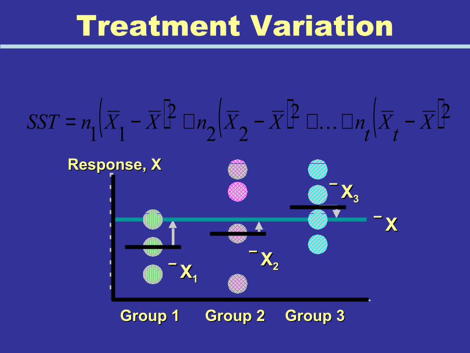
Treatment Variation

XX

XX33

XX22XX11



( ) ( ) ( )2222

211

XtXtnXXnXXnSST −++−+−=

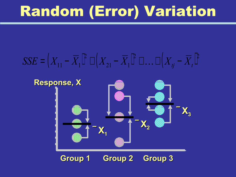
Random (Error) Variation

XX22XX11

XX33



( ) ( ) ( ) 22

121

2

111 ttj XXXXXXSSE −++−+−=

SStotal=SSerror+SStreatment

Error Variation

SSE=SStotal-SStreatment

The design model

where Yij is a random variable denoting the (ij)th observation, µ

is a parameter common to all treatments called the overall mean,

τi is a parameter associated with the ith treatment called the ith

treatment effect, and εij is a random error component.

==++=

nj

aiY ijiij ,.......,2,1

,....,2,1ετµ

Completely Randomized Design


This is an example of a completely randomized single-

factor experiment with four levels of the factor.

The levels of the factor are called treatments, and each

treatment has six observations or replicates.

This figure indicates that changing the hardwood

concentration has an effect on tensile strength; specifically,

higher hardwood concentrations produce higher observed

tensile strength.

Analysis of Variance

Suppose we have a different levels of a single factor that we

wish to compare.

The response for each of the a treatments is a random variable.

Let yij, represents the jth observation taken under treatment i.

We initially consider the case in which there are an equal

number of observations, n, on each treatment.


We are interested in testing the equality of the a

treatment means µ1 , µ2 ,..., µa .We find that this is

equivalent to testing the hypotheses

If the null hypothesis is true, each observation consists of

the overall mean µ plus a realization of the random error

component εij and changing the levels of the factor has no

effect on the mean response.

ioneleastatforH

H

ia

a

0:

0.....: 210

≠====

ττττ

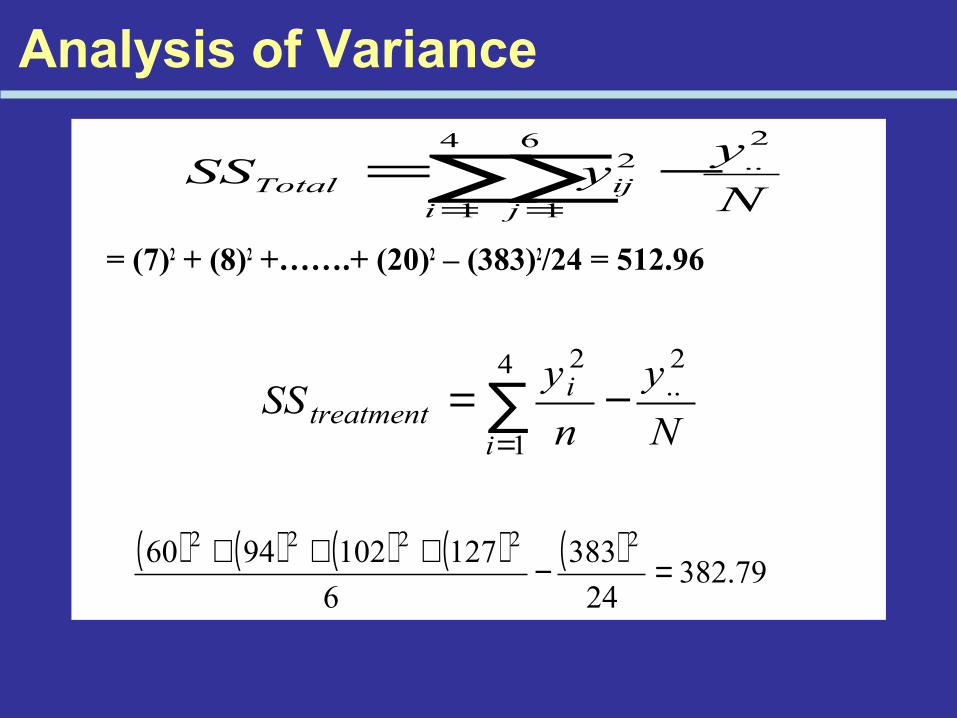
Analysis of Variance The sum of square total is

The sum of square treatment is

The error sum of squares is

SSError = SSTotal - SSTreatment

N

yySS

a

i

n

jijT

2..

1 1

2 −=∑∑= =

N

y

n

ySS

a

i

itreatment

2..

1

2

−= ∑=


The ANOVA partitions the total variability in the sample

data into two component parts.

Then, the test of the hypothesis is based on a

comparison of two independent estimates of the population

variance.

The total variability in the data is described by the total

sum of squares.


We can show that if the null hypothesis H0 is true, the

ratio has an F-distribution with a - 1 and a(n - 1) degrees of

freedom.

If the null hypothesis is false, the expected value of

MSTreatments is greater than σ2.

We would reject H0 if F >F∞,a-1,a(n-1).

( )( )[ ] E

Treatmant

E

Treatment

MS

MS

naSS

aSSF =

−−=1/

1/


Example. In the paper tensile strength experiment,

we can use the ANOVA to test the hypothesis that

different hardwood concentrations do not affect the

mean tensile strength of the paper.

The hypotheses are

H0: τ1= τ2= τ3= τ4= 0

Ha: τi ≠ 0 for at least one


= (7)2 + (8)2 +…….+ (20)2 – (383)2/24 = 512.96

N

yySS

i jijTotal

2..

4

1

6

1

2 −=∑∑= =

N

y

n

ySS

i

itreatment

2..

4

1

2

−= ∑=

( ) ( ) ( ) ( ) ( )79.382

24

383

6

1271029460 22222

=−+++

treatmenttotalerror SSSSSS −=

SSerror = 512.96 - 382.79 = 130.17



The typical ANOVA table for CRD

Source ofVaraition

Sum of Squares

Degree ofFreedom

Mean Square

F

Treatment SSTreatment a-1 MSTreatment

MSTreatment

MSError

Error SSError a(n-1( MSError

Total SSTotal an-1

Source ofVaraition

Sum of Squares

Degree ofFreedom

Mean Square

F

Hardwoodconcentration

382.79 3 127.60 19.60

Error 130.17 20 6.51

Total 512.96 23



SSE = SST – SStreatment

= 512.96 – 382.79 = 130.17

From ANOVA results, we will reject H0, if F > FTable

F = 127.60 / 6.51 = 19.60

F0.01, 3, 20 = 4.94

Therefore, we reject H0 and conclude that

hardwood concentration affectsaffects the mean strength of

the paper.

Multiple Comparisonsand mean separation

by LSD

Multiple Comparisons

When the null hypothesis is rejected in the ANOVA, we

know that some of the treatment or factor level means are

different.

However, the ANOVA doesn’t identify which means are

different.

Methods for investigating this issue are called multiple

comparisons methods.

Fisher’s least significant difference (LSD) method.


where LSD, the least significant difference, is

If the sample sizes are different in each treatment, the

LSD is

n

MStLSD E

na

2(1(,2/ −= α

+= −

jiEaN nn

MStLSD11

,2/α

Multiple Comparisons Ex. Apply the Fisher LSD method to the hardwood concentration

experiment. There are a = 4, n = 6, MSE = 6.51, with 95 %

confidence interval and t0.025,20 = 2.086. The treatment means are

The value of LSD is

17.21

00.17

67.15

00.10

.4

.3

.2

.1

====

y

y

y

y

07.36/(51.6(2086.2/220,025.0 ==nMSt E

Source ofVaraition

Sum of Squares

Degree ofFreedom

Mean Square

F

Hardwoodconcentration

382.79 3 127.60 19.60

Error 130.17 20 6.51

Total 512.96 23


Multiple Comparisons Therefore, any pair of treatment averages that differs by more

than 3.07 implies that the corresponding pair of treatment means

are different.

The comparisons among the observed treatment averages are

4 vs. 1 = 21.17 – 10.00 = 11.17 > 3.07

4 vs. 2 = 21.17 – 15.67 = 5.50 > 3.07

4 vs. 3 = 21.17 – 17.00 = 4.17 > 3.07

3 vs. 1 = 17.00 – 10.00 = 7.00 > 3.07

3 vs. 2 = 17.00 – 15.67 = 1.33 < 3.07

2 vs. 1 = 15.67 – 10.00 = 5.67 > 3.07


From this analysis, we see that there are significant

differences between all pairs of means except 2 and 3.

This implies that 10 and 15% hardwood concentration

produce approximately the same tensile strength and that

all other concentration levels tested produce different

tensile strengths.

Designs

2- Randomized Complete Block Design

(RCBD)

• divides the group of experimental units into n homogeneous groups of size t.

• These homogeneous groups are called blocks.

• The treatments are then randomly assigned to the experimental units in each block - one treatment to a unit in each block.

RCBD

Example 1: • Suppose we are interested in how weight gain

(Y) in rats is affected by Source of protein (Beef, Cereal, and Pork) and by Level of Protein (High or Low).

• There are a total of t = 3×2 treatment combinations of the two factors (Beef -High Protein, Cereal-High Protein, Pork-High Protein, Beef -Low Protein, Cereal-Low Protein, and Pork-Low Protein) .

RCBD

• Suppose we have available to us a total of N = 60 experimental rats to which we are going to apply the different diets based on the t = 6 treatment combinations.

• Prior to the experimentation the rats were divided into n = 10 homogeneous groups of size 6.

• The grouping was based on factors that had previously been ignored (Example - Initial weight size, appetite size etc.)

• Within each of the 10 blocks a rat is randomly assigned a treatment combination (diet).

RCBD

• The weight gain after a fixed period is measured for each of the test animals and is tabulated on the next slide:

RCBD

Block Block 1 107 96 112 83 87 90 6 128 89 104 85 84 89 (1) (2) (3) (4) (5) (6) (1) (2) (3) (4) (5) (6)

2 102 72 100 82 70 94 7 56 70 72 64 62 63 (1) (2) (3) (4) (5) (6) (1) (2) (3) (4) (5) (6)

3 102 76 102 85 95 86 8 97 91 92 80 72 82 (1) (2) (3) (4) (5) (6) (1) (2) (3) (4) (5) (6)

4 93 70 93 63 71 63 9 80 63 87 82 81 63 (1) (2) (3) (4) (5) (6) (1) (2) (3) (4) (5) (6)

5 111 79 101 72 75 81 10 103 102 112 83 93 81 (1) (2) (3) (4) (5) (6) (1) (2) (3) (4) (5) (6)

RCBD

Example 2: • The following experiment is interested in

comparing the effect four different chemicals (A, B, C and D) in producing water resistance (y) in textiles.

• A strip of material, randomly selected from each bolt, is cut into four pieces (samples) the pieces are randomly assigned to receive one of the four chemical treatments.

RCBD

• This process is replicated three times producing a Randomized Block (RB) design.

• Moisture resistance (y) were measured for each of the samples. (Low readings indicate low moisture penetration).

• The data is given in the diagram and table on the next slide.

RCBD

Diagram: Blocks (Bolt Samples)

RCBD

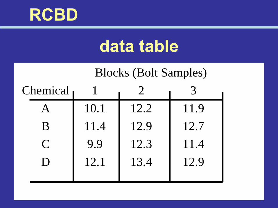
Blocks (Bolt Samples)

Chemical 1 2 3

A 10.1 12.2 11.9

B 11.4 12.9 12.7

C 9.9 12.3 11.4

D 12.1 13.4 12.9

data table

RCBD

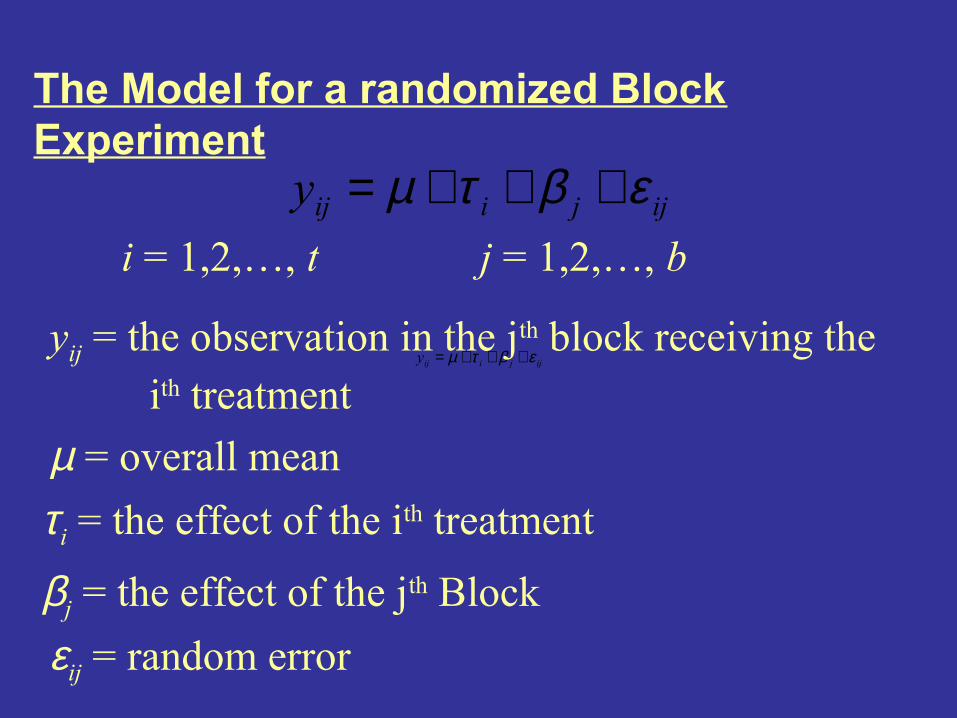
The Model for a randomized Block Experiment

ijjiijy εβτµ +++=

ijjiijy εβτµ +++=i = 1,2,…, t j = 1,2,…, b

yij = the observation in the jth block receiving the ith treatment

µ = overall mean

τi = the effect of the ith treatment

βj = the effect of the jth Block

εij = random error

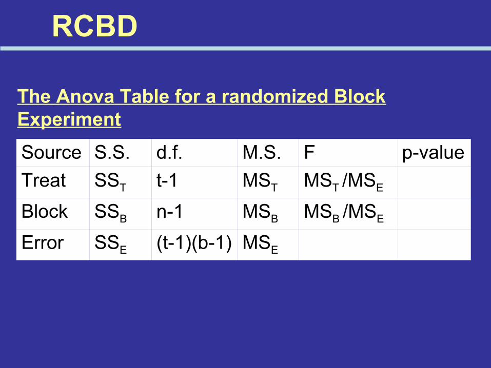
The Anova Table for a randomized Block Experiment

Source S.S. d.f. M.S. F p-value

Treat SST t-1 MST MST /MSE

Block SSB n-1 MSB MSB /MSE

Error SSE (t-1)(b-1) MSE

RCBD

• A randomized block experiment is assumed to be a two-factor experiment.

• The factors are blocks and treatments.

• The is one observation per cell. It is assumed that there is no interaction between blocks and treatments.

• The degrees of freedom for the interaction is used to estimate error.

RCBD

The ANOVA Table for Diet Experiment

Source S.S d.f. M.S. F p-valueBlock 5992.4167 9 665.82407 9.52 0.00000Diet 4572.8833 5 914.57667 13.076659 0.00000

ERROR 3147.2833 45 69.93963

The Anova Table for Textile Experiment

SOURCE SUM OF SQUARES D.F. MEAN SQUARE F TAIL PROB.Blocks 7.17167 2 3.5858 40.21 0.0003Chem 5.20000 3 1.7333 19.44 0.0017

ERROR 0.53500 6 0.0892

• If the treatments are defined in terms of two or more factors, the treatment Sum of Squares can be split (partitioned) into: – Main Effects– Interactions

The ANOVA Table for Diet Experiment terms for the main effects and interactions

between Level of Protein and Source of Protein

Source S.S d.f. M.S. F p-valueBlock 5992.4167 9 665.82407 9.52 0.00000Diet 4572.8833 5 914.57667 13.076659 0.00000

ERROR 3147.2833 45 69.93963

Source S.S d.f. M.S. F p-valueBlock 5992.4167 9 665.82407 9.52 0.00000

Source 882.23333 2 441.11667 6.31 0.00380Level 2680.0167 1 2680.0167 38.32 0.00000

SL 1010.6333 2 505.31667 7.23 0.00190ERROR 3147.2833 45 69.93963

H.W

- Latin Square Factorial Design Split-plot design

Advantages and disadvantages of each disign

95720357 a-design-of-experiments

Automotive