94 ieee transactions on robotics, vol. 26, no. 1, …96 ieee transactions on robotics, vol. 26, no....

94 IEEE TRANSACTIONS ON ROBOTICS, VOL. 26, NO. 1, FEBRUARY 2010

Online Trajectory Generation: Basic Concepts forInstantaneous Reactions to Unforeseen Events

Torsten Kroger, Member, IEEE, and Friedrich M. Wahl, Member, IEEE

Abstract—This paper introduces a new method for motion-trajectory generation of mechanical systems with multiple degreesof freedom (DOFs). The key feature of this new concept is thatmotion trajectories are generated online, i.e., within every controlcycle, typically every millisecond. This enables systems to reactinstantaneously to unforeseen and unpredictable (sensor) eventsat any time instant and in any state of motion. As a consequence,(multi)sensor integration in robotics, in particular the developmentof control systems enabling sensor-guided and sensor-guarded mo-tions, becomes greatly simplified. We introduce a class of onlinetrajectory-generation algorithms and present the mathematical ba-sics of this new approach. The algorithms presented here consist ofthree steps: calculation of the minimum synchronization time forall DOFs, synchronization of all DOFs, and calculation of outputvalues. The theory is followed by real-world experimental resultsindicating new possibilities in robot-motion control.

Index Terms—Hybrid switched systems, multisensor integra-tion, robot-motion control, trajectory generation.

I. INTRODUCTION

THIS PAPER focuses on sensor integration in robotics,in particular in robotic-manipulation control systems. We

consider a mechanical system with multiple degrees of freedom(DOFs) equipped with one or more sensors delivering digitaland/or analog sensor signals. It is—of course—no matter ofquestion that sensor integration and sensor-based control be-long to the very basics in robotics. However, there is still oneimportant question that has yet to be completely answered: Ifwe consider a robot in an arbitrary state of motion, how canwe calculate a trajectory if we want the robot to react instan-taneously to unforeseen sensor events? This is comparable tomany human everyday life scenarios: If a little child acciden-tally touches a stove with its hand, he or she knee-jerkily reactsby pulling its hand away from the hot surface. Another scenariocould be the fight of two swordsmen: Depending on the motionof the opponent, the fighters react immediately by adapting theirown body motions and moves.

Before coming up with details, we would like to make somebasic clarifications: A robotic system is considered as a mechan-ical and/or mobile system with multiple DOFs. Assuming sucha system to be equipped with a number of (different) sensors,we distinguish between

Manuscript received April 15, 2009; revised October 6, 2009 and October 19,2009. First published December 8, 2009; current version published February9, 2010. This paper was recommended for publication by Associate EditorA. Albu-Schaffer and Editor J.-P. Laumond upon evaluation of the reviewers’comments.

The authors are with the Institut fur Robotik und Prozessinformatik, Tech-nische Universitat Carolo-Wilhelmina zu Braunschweig, Muhlenpfordtstraße23, D-38106 Braunschweig, Germany (e-mail: [email protected]; [email protected]).

Digital Object Identifier 10.1109/TRO.2009.2035744

Fig. 1. Subject of this paper: Instantaneous switchings between trajectory-following motions and sensor-guided motions.

1) trajectory-following control;2) sensor-guided motion control;3) sensor-guarded motion control.Sensor-guided motion control employs the system’s actuators

to be part of a control loop, whose control variables are basedon sensor signals (cf. Fig. 1). We consider a sensor as a genericdevice that delivers a signal depending on the overall systemstate, i.e., the robotic system with its complete environment.Clear and concrete examples are force/torque control (e.g., [1],just to name one out of many) and visual servo control (e.g., [2]).Here, the robot motion of one single control cycle depends onthe sensor signal(s) of the current control cycle.

In contrast to this, sensor-guarded motions are consideredas trajectory-following motions and/or sensor-guided motions(cf. Fig. 1), whose motion parameters may change abruptly,depending on sensor events. These parameter changes may in-clude set-point switchings for closed-loop controllers (e.g., newforce/torque control set-points) as well as new target positionsfor trajectory-following control. Simple examples here are thetransition from free space to contact, i.e., the transition frompose to force/torque control. In the moment of transition, therobot controller switches the controllers for all DOFs being incontact from trajectory-following control to force/torque con-trol. A second obvious example is the instantaneous reactionof a robotic system to any predictable or unpredictable event:The manipulator of [3] plays the parlor game Jenga [4] andhas to interrupt any motion as soon as the game tower starts totopple.

In the development of such systems, it becomes evident thatwe need to switch discretely between several (open- and/orclosed-loop) continuous controllers at any time. If we arbitrarilyswitch one or more DOFs from trajectory-following controlto sensor-guided control, this problem is usually solved. Byusing the transfer function of a desired controller, commandvariables for lower level control can be generated at any timeinstant (cf. Fig. 1). However, how can we switch one, some,or all DOFs of a robotic system from sensor-guided control

1552-3098/$26.00 © 2009 IEEE

Authorized licensed use limited to: Stanford University. Downloaded on March 01,2010 at 15:15:26 EST from IEEE Xplore. Restrictions apply.

KROGER AND WAHL: ONLINE TRAJECTORY GENERATION: BASIC CONCEPTS FOR INSTANTANEOUS REACTIONS TO UNFORESEEN EVENTS 95

to trajectory-following control? If we consider a robot in anarbitrary state of motion, how can we calculate a trajectory if wewant the robot to react instantaneously to unforeseen (sensor)events?

This is the central question of this paper, whose central nov-elty is an open-loop control module that is able to generatetime-optimal and time-synchronized motion trajectories for me-chanical systems with multiple DOFs during runtime, i.e., on-line during every control cycle. This opens completely newadvances for multisensor integration in robotic systems, and hy-brid switched-control systems become suited for a wide rangeof robotic applications.

Let us now give a short overview of this paper: After relatedworks have been presented in Section II, Section III introducessome basics, a dedicated notation for this paper, and some spe-cial conventions used throughout the paper. During the develop-ment of this paper, nine different types of online trajectory gen-erators (OTG) were elaborated and are classified in Section IV.The basic algorithm applied to any type of online trajectory gen-eration is introduced in Section V, whereas Section VI describesthe most relevant type of OTG, i.e., Type IV. After the relation ofthis new concept to higher-level (sensor-based) motion-planningsystem is discussed in Section VII, Section VIII presents simu-lation and real-world experimental results, which highlight thepractical relevance of this concept.

II. RELATED WORK

Off-Line Trajectory-Generation Concepts: Kahn and Roth [5]belong to the pioneers in the field of time-optimal trajectoryplanning. They used methods of optimal, linear control theoryand achieved a near-time-optimal solution for linearized manip-ulators. The work of Brady [6] introduces several techniques oftrajectory planning. In later works, the manipulator dynamicswere taken into account [7], and jerk-limited trajectories wereapplied [8]. The concept of Lambrechts et al. [9] produces very-smooth fourth-order trajectories but is also limited to a knowninitial state of motion and to one DOF.

Real-Time Adaptive-Motion Planning: In recent times, workson real-time adaptive-motion planning have been published[10]–[13]. Here, the field of online trajectory planning is ad-dressed and the path of a robotic manipulator is adapted thatdepends on its state and environment. This proposal focuseson online trajectory generation, which is more related to thefield of robot control. It acts as an important interface to suchhigher-level planning methods of [10]–[13] (cf. Section VII).

Online Trajectory-Generation Concepts: The works mostlyrelated to this paper are [14]–[19]. Macfarlane and Croft [14]present a jerk-bounded, near-time-optimal trajectory plannerthat uses quintic splines, which are also computed online butonly for 1-DOF systems. In [15], Cao et al. use rectangularjerk pulses to compute trajectories, but accelerations differentfrom zero cannot be applied. Compared with the multi-DOFapproach presented here, the latter method has been developedfor 1-D problems only. Broquere et al. [16] published a workthat uses an online trajectory generator for an arbitrary numberof independently acting DOFs. The approach is very similar to

the one of Liu [17] and is based on the classic seven-segmentacceleration profile [20], but the approach is unfortunately alsoincomplete and can only perform reactions if the current accel-eration value of a DOF is zero. Briefly summarized, a majordisadvantage of [14]–[17] is that they cannot cope with initialacceleration values unequal to zero. A further, very recent workof Haschke et al. [18] presents an online trajectory planner inthe very same sense as this paper does. The proposed algorithmgenerates jerk-limited trajectories from arbitrary states of mo-tion, but it suffers from numerical stability problems, i.e., itmay happen that no jerk-limited trajectory can be calculated.In such a case, a second-order trajectory with infinite jerks iscalculated. Furthermore, the algorithm only allows target ve-locities of zero. Ahn et al. [19] proposed a work for the onlinecalculation of 1-D trajectories for any given state of motionand with arbitrary target states of motion, i.e., with target ve-locities and target accelerations unequal to zero. Sixth-orderpolynomials are used to represent the trajectory, which is calledarbitrary-states polynomial-like trajectory (ASPOT). The majordrawback of this paper is that no kinematic-motion constraints,such as maximum velocity, acceleration, and jerk values, can bespecified.

Concepts for Instantaneous Reactions to Collisions and Inter-actions: Heinzmann and Zelinsky [21] introduced a method tolimit impact forces in the case of undesired collisions, such thatdamage and possible human injuries are prevented. Based on theskeleton algorithm [22], De Santis and Siciliano [23] present areactive method for collision avoidance in which propriocep-tive sensor data are used to calculate repulsion forces and jointtorques to “flee” from the position in which a potential collisionis expected. Based on these works, Haddadin et al. [24] presenta very impressive work on the detection of unforeseen collisionsand respective reaction concepts. Five different collision (= sen-sor event) reaction strategies are investigated: 1) no reaction; 2)immediate stopping; 3) switching from position control to zero-gravity torque control [25]; 4) switching to torque control withgravity compensation, but, in contrast, to; 3) using joint torquefeedback and the signal of the estimated external torque, whichis used as a collision signal, to scale down both the motor inertiaas well as the link inertia, thus obtaining an even “lighter” robot;and 5) using the estimated external torque to implement an ad-mittance controller. The strategies 3–5 contain switchings fromtrajectory-following control to sensor-guided robot motion con-trol; this paper considers the opposite way of switching: fromsensor-guided motion back to trajectory-following control (cf.Fig. 1) or abrupt switching of trajectory parameters (e.g., targetstate of motion and/or kinematic-motion constraints) to react tounforeseen events such as the detection of potential collisions.

The proposed class of algorithms of this paper closes theimportant loop of Fig. 1. Summarizing this section briefly, allmentioned approaches are not able to cope with arbitrary initialstates of motion, i.e., arbitrary position, velocity, and accel-eration values, in a robust way—neither for the one- nor forthe multidimensional case. This paper extends all mentionedworks, such that instantaneous reactions to unforeseen (sen-sor) events become feasible for multi-DOF robotic systems(cf. Fig. 1).



III. BASICS, NOTATIONS, AND CONVENTIONS

This section briefly introduces the nomenclature usedthroughout this paper, defines some important terms, and givesa first impression how the regarded trajectories are mathemati-cally represented.

As we consider PC- or microcontroller-based systems forrobot-motion control, we assume a time-discrete overall systemwith a set of time instants

T = {T0 , . . . , Ti, . . . , TN }with Ti = Ti−1 + T cycle and i ∈ {1, . . . , N} (1)

where T cycle represents the cycle time of the system. Time-discrete values are represented by capital letters, time-continuous values by lowercase letters. The position of therobotic system at time Ti is �Pi = (1Pi, . . . , kPi, . . . , K Pi)

T ,where K is the number of DOFs. Velocities, accelerations, andjerks are analogously represented by �Vi , �Ai , and �Ji . A completestate of motion at time Ti is described by the matrix

Mi = (�Pi, �Vi, �Ai, �Ji)

= (1 �Mi, . . . , k�Mi, . . . , K

�Mi)T . (2)

Kinematic-motion constraints are analogously denoted as

Bi = (�V maxi , �Amax

i , �Jmaxi , �Dmax

i ) (3)

where �Dmaxi is the maximum value for the derivative of jerk at

time Ti . A target state of motion is denoted by

M trgti = (�P trgt

i , �V trgti , �A trgt

i , �J trgti ). (4)

TN is the time instant at which Mtrgti will be reached. As we

will explain later, time-continuous polynomials are needed forthe internal representation of trajectories. Here

lk pi(t) = a4(t − ∆t)4 + a3(t − ∆t)3

+ a2(t − ∆t)2 + a1(t − ∆t) + a0 (5)

constitutes a fourth-order polynomial describing the positionprogression for DOF k, time-shifted by ∆t, and calculated attime instant Ti . The index l is described later in this section.Polynomials for velocity, acceleration, and jerk progressions areanalogously denoted by l�vi(t), l�ai(t), and l�ji(t). In summary,we obtain a matrix of polynomials

lmi(t) = (l �pi(t), l�vi(t), l�ai(t), l�ji(t))

= (l1 �mi(t), . . . , l

k �mi(t), . . . , lK �mi(t))T (6)

where a single row, i.e., the polynomials of one single DOF k,is denoted by

lk �mi(t) =

(lk pi(t), l

k vi(t), lk ai(t), l

k ji(t)). (7)

Each set of motion polynomials lmi(t) for all K DOFs is ac-companied by a set of time intervals

lVi ={

l1ϑi, . . . ,

lkϑi, . . . ,

lK ϑi

}, where l

kϑi =[l

kti ,

(l+1)k ti

]

(8)in which a set of polynomials l

k �mi(t) for one single DOF k isvalid. A complete motion trajectory Mi(t) is finally composed

of a set of motion polynomials with according time intervals

Mi(t) = {(1mi(t), 1Vi), . . . , (lmi(t), lVi),

. . . , (Lmi(t), LVi)}. (9)

Depending on the type and variant of OTG (cf. Section IV), theinitial state of motion M0 , and the target state of motion Mtrgt

0 ,the value L determines the required number of polynomials(i.e., the number of single trajectory segments) to describe thecomplete trajectory from M0 to Mtrgt

0 .One important property of OTG is that all DOFs, which are

selected for trajectory-following control, have to reach theirtarget state of motion Mtrgt

i at the same time instant, namely attsynci in order to achieve time synchronization. As a consequence

of this requirement, we can already state that

TN − tsynci ≤ T cycle . (10)

Just to give an impression of time dimensions, T cycle lies inthe range of one millisecond or less, i.e., the resulting OTGalgorithms are designed to be applicable on a very low controllevel.

In the following, the term time optimality is supposed to bedefined; we distinguish between the following two differentkinds:

1) Kinematic time-optimality: A system is transferred froman initial state of motion Mi at instant Ti into a desiredtarget state of motion Mtrgt

i within the shortest possibletime without any consideration of couplings between in-dividual DOFs.

2) Dynamic time-optimality: A system is transferred froman initial state of motion Mi at instant Ti into a desiredtarget state of motion Mtrgt

i within the shortest possibletime with consideration of the whole system dynamics.

In the context of this paper, kinematic time optimality is con-sidered. The important consequence of kinematic time optimal-ity is, that all K DOFs can be considered to be linearly indepen-dent. When calculating Mi(t) at Ti , the following requirementshave to be fulfilled to achieve time optimality:

∀ k ∈ {1, . . . , K}:1k ti = Ti

1k �mi(Ti) = k

�Mi

lk �mi(l

k ti) = l−1k

�mi(lk ti) with l ∈ {2, . . . , L}

Lk �mi(t

synci ) = k

�M trgti (11)

and

∀ (k, l) ∈ {1, . . . , K} × {1, . . . , L}:lk vi(t) ≤ kV max

i

lk ai(t) ≤ kAmax

i

lk ji(t) ≤ kJmax

i

lk di(t) ≤ kDmax

i

, with t ∈[l

kti ,

l+1k ti

](12)

such that

tsynci −→ min. (13)



Fig. 2. Example of a very simple case of a fourth-order motion trajectory forone DOF k consisting of L = 15 matrices of polynomials lmi (t) [cf. (6)]. Theinput parameters are k

�M0 = �0, k�B0 = (9.4 mm/s, 22.4 mm/s2 , 160 mm/s3 ,

2000 mm/s4 ), and k�M trgt

0 = (8.8 mm, 0 mm/s, 0 mm/s2 , and 0 mm/s3 )(cf. [9]).

Equation (11) describes the single-motion states at the beginningor at the end of a trajectory segment l, respectively. Due to (12),it is guaranteed that the motion variables are kept within theirkinematic constraints.

Now, we know how to describe a complete motion trajectoryMi(t) at a time instant Ti . It constitutes the minimum set ofparameters to handle sets of trajectories for OTG. For a betterunderstanding and to clarify these introductory equations, Fig. 2depicts a simple (translational) motion trajectory for one singleDOF k.

As last part of this section, we explain the accordance ofthese introductory description to the input and output values ofthe OTG algorithms. Fig. 3 shows all input parameters

Wi = (Mi ,Mtrgti ,Bi , �Si) (14)

and all output values Mi+1 of the OTG algorithm, where Wi

is an arbitrary (K × 13) matrix. The selection vector �Si is aBoolean vector and determines which of the K DOFs have tobe controlled by the OTG. The DOFs, which are controlled byother open- or closed-loop controllers, are not considered by thealgorithm.

Fig. 3. Input and output values the OTG (z−1 represents a hold element). Thedotted part indicates how the output values of the OTG are usually fed back.

We assume arbitrary values for Wi as granted; the only (triv-ial) kinematic constraint is given by (15)

∀ k ∈ {1, . . . ,K}:

kV trgti ≤ kV max

i ∧ kAtrgti ≤ kAmax

i ∧ kJ trgti ≤ kJmax

i . (15)

As already stated in (13), the challenge is to find a motiontrajectory Mi(t) that transfers the state of motion from Mi toMtrgt

i within the shortest possible time. For the current controlcycle at Ti , only Mi+1 is needed, because in the next controlcycle, we might have completely new input values Wi due to anunforeseen event or switching action. Hence, only Mi+1 is for-warded to the output. These values are then used as input valuesfor lower level control. This leads to the interesting requirementthat if the input values Mtrgt

i , Bi , and �Si remain constant fori ∈ {0, . . . , N}, and if the output values Mi+1 are directly fedback as input values for the following control cycle (cf. dottedpart of Fig. 3), then we have the following.

1) The value of the synchronization time must remain con-stant during the whole trajectory execution, i.e., tsync

i =const ∀ i ∈ {0, . . . , N}. This fact is relevant for time syn-chronization such that �V trgt

i , �Atrgti , and �J trgt

i are coin-stantaneously reached in �P trgt

i at tsynci .

2) All trajectories Mu (t) with u ∈ {1, . . . , N} must exactlyfit into the one of M0(t).

3) Furthermore, any trajectory Mu (t) with u ∈ {1, . . . , N}must exactly fit into all previously-calculated motion tra-jectories Mv (t) with v ∈ {0, . . . , u − 1}.

The general algorithm for the calculation of Mi(t) is de-scribed in Section V, but prior to this, we classify differenttypes and variants of OTG in the next section.



TABLE IDIFFERENT TYPES OF OTG

To summarize this section briefly, we introduced a dedicatednotation and described the task of OTG very generally withoutoffering solutions. Besides this, the important terms of time op-timality and time synchronization were clarified for the contextof this paper.

IV. TYPES AND VARIANTS OF ONLINE

TRAJECTORY GENERATION

This section defines different types and variants of OTG al-gorithms, i.e., the class of algorithms introduced by this paper.Depending on the type, the algorithmic complexity and the prac-tical relevance differ strongly.

A. Types of OTG

In general, we can denote that the output values of an OTGalgorithm are a function f of the input parameters, the OTGalgorithm itself is memoryless (it has no memory)

Mi+1 = f(Wi), where

f : IRαK × IBK −→ IRβK (16)

and IB = {0, 1} is responsible for the selection vector �Si . α andβ are type-dependent integer values. Table I shows a summaryof types of OTG. The OTG block of Fig. 3—if fully connectedto all input parameters and output values—corresponds to TypeIX. Depending on the type, not all input and output magnitudesare in use. Type VIII, for example, does not offer to specify�J trgti . Fig. 2, for example, shows a Type VI trajectory. β = 4

means that the position progression is described by polynomialsof up to fourth order, i.e., even the derivative of the jerk is lim-ited ( �Dmax

i ∈ IRK ). All further types are defined analogously.To finalize Table I, one may denote the trivial and irrelevant casewith rectangular velocity profiles as Type 0 (with α = 3, β = 1).Of course, it would also be possible to extend Table I by higherorder trajectories (Type X, XI, etc.), but the complexity stronglyincreases with increasing type numbers, such that the develop-ment of these algorithms is hardly possible. For clarification,this paper presents a whole class of algorithms that is applica-ble to all types of OTG; the higher order types (Types VI and

higher) are of theoretical character, but the Types I–V are highlyrelevant for sensor-based robot-motion control.

A very specific version of Type I was already suggested in [26]and works as well as Type II with unlimited jerks. These twotypes may offer sensor-integration possibilities for experimen-tal purposes, for example, in research institutions, but due tothe nonsmooth bang–bang or trapezoidal trajectory character-istics [27], they are not relevant for industrial practice, as hasalready been stated in [5]. To achieve long lifetimes for me-chanical systems, a jerk limitation is required (Types III–V).Compared with Type III, Types IV and V additionally pro-vide the possibility of specifying target-velocity vectors and/ortarget-acceleration vectors in space, which is important for theconsideration of system dynamics. As a result, Type IV is thefirst type of OTG, which is relevant for professional usage.

B. Variants of OTG

Regarding different variants of OTG, we distinguish betweenconstant and nonconstant kinematic constraint values and definetwo variants A and B as

A) Bi = const ∀ i ∈ Z

B) Bi �= const.The second, slightly more advanced variant with time-variant

values of kinematic motion constraints will be introduced ina follow-up publication and is important for the integration ofrobot dynamics in order to consider state-dependent and time-variant values of �Amax

i .

C. Positional Limits

The consideration of positional limits (k�Pmin

i , k�Pmax

i ) (e.g.,joint limits or Cartesian work space limits) cannot be embeddedin the OTG algorithm. In order to clarify this, Fig. 4 shows thecuboidal motion constraint space for the OTG Types III–V [cf.Table I and (3) and (12)] as well as the positional constraintskPmax

i and kPmini for one single DOF k at instant Ti . If we then

consider the current state of motion for this DOF k as

k�Mi = (kPi,+ kV max

i , 0, 0) (17)



Fig. 4. (Top) Kinematic motion constraints k�Bi of 1-DOF k at instant Ti for

the OTG Types III–V [cf. Table I and (3) and (12)], 3-D. (Bottom) Positionallimits, 1-D. The current state of motion for DOF k, k

�Mi , is marked by the whitecircle with the black dot in both diagrams [cf. (17)].

where kPi is very close to kPmaxi (cf. Fig. 4), we have the choice

to1) either overshoot kPmax

i and keep k�Mi within k

�Bi , or2) exceed k

�Bi and keep kPmaxi .

However, we cannot guarantee both (which is natural in thissituation). The requirement we have for practical implementa-tions is that we have to react to sensor events at unforeseen in-stants and in arbitrary states of motion. Hence, the responsibilityof keeping kPi within [kPmin

i , kPmaxi ] for all k ∈ {1, . . . , K}

is transferred to the system (or user) above the layer of the OTGalgorithm (e.g., a task or high-level motion planner). As also de-scribed in [14]–[18], it is the task of the OTG layer to move one,some, or all DOFs of a robotic system from an initial position �Pi

to a target position �P trgti , and the system above is responsible

for the (trivial) fact that

kP trgti ∈

[kPmin

i , kPmaxi

]∀ k ∈ {1, . . . , K} (18)

for the OTG Types I, III, and VI [cf. (15) and Table I). Forother OTG types, (18) becomes extended, because case differ-entiations have to be made. This topic will be investigated inSection VII.

V. ONLINE TRAJECTORY GENERATOR ALGORITHM—GENERAL

VERSION

Sections III and IV introduced basics, requirements, and typesof OTG. This section applies these foundations and describes thecentral OTG algorithm generally, such that it is applicable to alltypes and variants of OTG. To clarify its usage, Section VI de-tails the algorithm concretely by means of Type IV and presentspractical results.

Assuming the algorithm is called at a discrete time instant Ti ;all types of OTG require the same three algorithmic steps:

Step 1: calculation of the minimum possible tsynci ;

Step 2: synchronization of all selected DOFs to tsynci and

calculation of Mi ;Step 3: calculation of Mi+1 based on Mi .These steps are depicted in Fig. 5, which shows the overall

structogram of the OTG algorithm. The following three sectionsdescribe each step in detail.

Fig. 5. Nassi–Shneiderman structogram of the general OTG algorithm.

A. Step 1

This step is the most complex one, although it only computesthe synchronization time tsync

i , i.e., one scalar value. It is afunction

f : IRαK × IBK −→ IR. (19)

As can be seen in Fig. 5, Step 1 can be subdivided into three parts:the individual calculation of the minimum execution time k tmin

i

for each selected DOF k; the calculation of possibly existinginoperative time intervals kZi , in which a selected DOF cannotbe synchronized; and finally, the determination of tsync

i .1) Minimum Execution Time: One of the key ideas of this

algorithm is that there is a finite set of possible motion profiles ofwhich one profile transfers one single selected DOF k from theinitial state of motion k

�Mi to its target state of motion k�M trgt

i

within the shortest possible time k tmini (time optimally). This

finite set for Step 1 is denoted by

PStep1 ={1ΨStep1 , . . . , rΨStep1 , . . . , RΨStep1} (20)

where R is the number of elements inPStep1 and depends on thetype of OTG. A concrete profile is denoted by rΨStep1 . Whatkinds of motion profiles are considered also depends on the usedtype of OTG:

Types I–II : Velocity profiles (β = 2)

Types III–V : Acceleration profiles (β = 3)

Types V–IX : Jerk profiles (β = 4).

It is the task of this substep to execute a function f : IRα −→PStep1 for every single selected DOF in order to select themotion profile which leads to the time-optimal trajectory andwhich simultaneously determines k tmin

i for each DOF k. Oncethe time-optimal profile kΨStep1

i has been selected for 1-DOFk, a system of nonlinear equations can be set up and solved tocalculate k tmin

i . The selection of kΨStep1i can be realized by

decision trees, which are exemplarily presented in Section VI.1

1Alternatively, one could set up R systems of nonlinear equations, calculateall solutions, take all valid solutions for k tm in

i , and choose the minimum one.However, this procedure is computationally too expensive, especially if lowvalues for T cycle are desired.



Each motion profile rΨStep1 with r ∈ {1, . . . , R} leads to asystem of nonlinear equations, and each system is solvable fora certain domain rDStep1 with

rDStep1 ⊂ IRα . (21)

For the decision tree implementing (19), it is absolutely essentialthat

R⋃

r=1

rDStep1 ≡ IRα (22)

holds. If this is not the case, the tree is erroneous, and thealgorithm will not work for certain input parameters, whichwould be unacceptable for its practical application. In the workof Broquere et al. [16] as well as in the contribution of Liu [17],which suggest similar approaches for 1-DOF systems, (22) doesnot hold, and hence, these approaches are not applicable ingeneral, but only for some (practically hardly relevant) specialcases.

Not even the theoretic literature provides a concept to letonly 1-DOF react instantaneously to unforeseen events withjerk-limited trajectories. In this paper, we implicitly introduceboth, the 1-D case as well as the multidimensional case. If only1-DOF is considered, the solution of the system of equations forthe time-optimal motion profile kΨ

Step1i contains all required

trajectory parameters to set up Mi . The multidimensionalcase, which also requires synchronization, is introduced in thefollowing.

2) Inoperative Time Intervals: After the minimum executiontime k tmin

i has been calculated, we have to check whether it ispossible to execute the trajectory for this DOF k within anytime t >k tmin

i . If this is the case, no inoperative time intervalskZi = {} are existent; depending on the type, kZi may containup to Z = 3 time intervals in which a selected DOF k cannot besynchronized. Referring to Table I, this can be expressed by

Z = α − 2β − 1 (23)

such that the following values of Z appear:

Types I, III, VI : Z = 0

Types II, IV, VII : Z = 1

Types V, VIII : Z = 2

Type IX : Z = 3.

If only a target position vector �P trgti is given (Types I, III,

and VI), the target state can, of course, be reached at any timet ≥ tmin

i . For every further target-motion state vector, one in-operative time interval may occur, i.e., if an additional targetvelocity vector �V trgt

i is specified (Types II, IV, and VII) oneinoperative time interval may be present (cf. Fig. 6); a targetacceleration vector �Atrgt

i (Types V and VIII) leads to up to twoinoperative time intervals, etc. The inoperative time intervals ofone single DOF may overlap such that two or more intervalsaffiliate to one interval.

The single elements of kZi are then denoted by

zk ζi =

[z

ktbegini , z

k tendi

], with z ∈ {1, . . . , Z}. (24)

Fig. 6. Example of an inoperative time interval for one translational DOFk calculated by a Type II OTG. Assuming k Am ax

i = 20 mm/s2 , k�Mi =

(50 mm, 80 mm/s, 0, 0), and k�M trgt

i = (300 mm, 70 mm/s, 0, 0), the time-optimal case would take k tm in

i = 2820 ms. If other DOFs require more time,

this DOF k can also reach k�M trgt

i after 1k tb egin

i = 4950 ms, but it is not

possible to transfer DOF k to k�M trgt

i in a time 1k tb egin

i < t <1k tend

i with1k tend

i = 10, 050 ms. For all times t ≥1k tend

i , the synchronized execution ofDOF k is possible again. As a result for DOF k, there is an inoperative timeinterval of 1

k ζi = [4950 ms, 10, 050 ms].

Fig. 7. Example of the determination of tsynci for K = 4 DOFs. Here,

tsynci = 1

2 tendi .

To explain the origin of these inoperative time intervals, Fig. 6illustrates a simple Type II trajectory with simple bang–bangcharacteristics and one inoperative time interval 1

k ζi . It is ab-solutely essential that the OTG algorithm be able to providea solution for any set of input values Wi . If this could notbe guaranteed, the concept would not be complete, would beunsafe, and, thus, would be practically irrelevant. As a result,2Z + 1 = 2α − 4β − 1 decision trees are required for Step 1,i.e., one tree for the calculation of tsync

i and two Z trees for thecalculation of z

k ζi ∀ z ∈ {1, . . . , Z}.3) Determining tsync

i : After the minimum execution timesfor all selected DOFs and all existing inoperative time intervalshave been calculated, tsync

i can be determined easily. First, thegreatest time of all minimum execution times is taken. tsync

i

cannot be less than this value. As second step, we have to regardthat tsync

i must not be part of any inoperative time intervalzk ζi with (z, k) ∈ {1, . . . , Z} × {1, . . . ,K}. Fig. 7 illustratesan example with four DOFs, where tsync

i is determined.



B. Step 2

The purpose of this step is to set up all parameters of thetrajectory Mi calculated at Ti [cf. (6)–(9)]. Wi and tsync

i act asinput parameters for this second step. Due to Step 1, we alreadyknow that all selected DOFs are able to reach their desiredtarget state of motion Mtrgt

i exactly at tsynci without exceeding

the kinematic-motion constraints Bi . Here, a similar procedureas in the first part of Step 1 is applied. The key idea that there is afinite set of motion profiles to set up the final motion trajectoriesis employed again. This setPStep2 differs from the one of Step 1:PStep1

PStep2 ={1ΨStep2 , . . . , sΨStep2 , . . . , S ΨStep2} (25)

where S denotes the number of elements in PStep2 and de-pends on the type of OTG. According to Table I, a functionf : IRα+1 −→ PStep2 is required, which determines a motionprofile for each selected DOF k. This function is again repre-sented by a decision tree, which will be briefly described in thenext section. After the correct motion profile kΨStep2

i is chosenfor a DOF k, another system of nonlinear equations can be setup.

According to Table I, a decision tree that acts as function

f : ((IRα+1)\ H) −→ PStep2 (26)

is required, which determines a motion profile sΨStep2 for eachselected DOF k. The meaning of H, i.e., holes in the domainspace, will be described next. Compared with Step 1, Step 2always requires only one decision tree, which is executed oncefor every selected DOF and control cycle. However, comparedwith Step 1, there are two significant differences.

1) While in Step 1, more than one system of equations mayachieve a valid solution, and in Step 2, only one element ofPStep2 leads to a solvable system of equations. This fact isrooted in the nature of the Step 2 motion profiles and leadsto a deterministic behavior, i.e., there can always be onlyone possible trajectory, which transfers a selected DOF kfrom k

�Mi to k�M trgt

i in tsynci .

2) If we denote the input domain of the system of equationsthat corresponds to the motion profile sΨStep2 as

sD Step2 ⊂ IRα+1 (27)

we do not have such an equivalence as described by (22)for Step 1

S⋃

s=1

sDStep2 �≡ IRα+1 . (28)

Due to the inoperative time intervals kZi for each selectedDOF k, the (α + 1)-dimensional space contains holes, inwhich none of the systems of equations that correspondto the motion profiles of PStep2 is solvable and in whichthe decision tree of (26) does not deliver a solution. Theseholes in the (α + 1)-dimensional space are represented bythe set

H ⊂ IRα+1 . (29)

Fig. 8. Two-dimensional illustration of (30). Union of all input domainssDStep2 of the systems of equations for the motion profiles of Step 2: PStep2 .The black areas represent H.

As a result, the union of all input domains of the systemsof equations for the Step 2 motion profiles PStep2 canbe described in (30); this is illustrated by Fig. 8. We canalso logically conclude here that the set of holes H isdisjunctive with the union of all input domains

S⋃

s=1

sDStep2 = (IRα+1)\H. (30)

Furthermore, it is an important property that the union ofpairwise intersections of all Step 2 input domains

S =S⋃

s=1

{sDStep2 ∩ uDStep2 ∀ u ∈ {1, . . . , S}∣∣u �= s

}

(31)

constitutes α-dimensional hyperplanes in the (α + 1)-dimensional space. These hyperplanes are described indetail by the decision tree of (26). The fact that S rep-resents only hyperplanes in the input space of Step 2 isessential for the deterministic behavior of the OTG algo-rithm, because this way there is only one possible motionprofile for any set of input values. If the (α + 1) inputvalues for a selected DOF k are an element of S, two oreven more motion profiles will lead to a solvable systemof equations, but the solution will be exactly the same forall profiles. This fact emphasizes the overall consistencyof the proposed concept.

Let us now answer the following question: How can we de-scribe the set of holes H? This is an important question becausewe have to prevent from entering such a hole. Entering a holewould lead to an unsolvable problem, and no output valuesMi+1 could be calculated.

The (α + 1)-dimensional space for one DOF k is spannedby the first α elements of k

�Wi and by the synchronization timetsynci . The values of k

�Wi can be arbitrary [cf. (14)]. Hence, theonly parameter that can be responsible for H is tsync

i , whichwas determined in Step 1. As described there, we need 2Zdecision trees to determine the limits of all inoperative timeintervals z

k ζi with (z, k) ∈ {1, . . . , Z} × {1, . . . , K}. These 2Zdecision trees exactly describe the set of holes H because wemask the codomain of tsync

i and, thus, the (α + 1)-dimensionalinput space.

An important insight at this point is that all (2Z + 1) decisiontrees of Step 1 and the decision tree of Step 2 must exactly fit



each other. It is comparable with a multidimensional puzzlegame whose parts have to fit each other exactly, and if this werenot the case, the game would not come to an end. The sameholds for the OTG algorithm: If the (2Z + 1) Step 1 decisiontrees do not fit each other, the algorithm will be erroneous, andthere will exist input values Wi , to which no output values canbe calculated.

The resulting solution of the nonlinear system of equations en-ables us to set up all L trajectory segments l

k �mi ∀ l ∈ {1, . . . , L}as well as all corresponding time intervals l

kϑi ∀ l ∈ {1, . . . , L}[cf. (5), (6), and (8)]. If this is done for all selected DOFs, Mi

is calculated for this time step Ti [cf. (9)].

C. Step 3

This third step of the OTG algorithm is trivial. After the com-plete trajectory for one time step Ti , Mi , has been calculatedin Step 2, we only have to find the valid time interval l

k ϑi withl ∈ {1, . . . , L} such that

l−1k ti ≤ (Ti + T cycle) ≤ l

k ti (32)

is satisfied [cf. (8) and (9)]. The output values Mi+1can finallybe calculated by

Mi+1 = lmi(Ti + T cycle). (33)

D. Final Remarks on the General OTG Algorithm

This section introduced the general OTG algorithm for alltypes and variants of OTG. Its complexity strongly depends onthe implemented type; the higher the roman number of the OTGtype, the higher its algorithmic complexity. The measure ofcomplexity is influenced, in particular, by two properties: 1) thesize of the decision trees in Steps 1 and 2 and 2) the solvability ofthe systems of equations, which are generated from the elementsin PStep1 and PStep2 . Over the past few years, implementationsof Types I–IV were realized by the authors, where Type IV isthe first one, which is relevant for practical usage. This typeincludes Types I–III (cf. Table I) and will be concretized in thenext section.

VI. TYPE IV ONLINE TRAJECTORY GENERATION

Compared to the general OTG algorithm in Section V, thissection exemplarily introduces one concrete type of OTG: TypeIV-A. This leads us to the following general parameters forthe algorithm: α = 8, β = 3, �A trgt

i = �0 ∧ �J trgti = �0 ∀ i ∈ Z;

in addition, �Dmaxi may contain infinite values for any i ∈ Z.

In simple words, this type achieves kinematically time-optimaland time-synchronized trajectories, whose velocity, accelera-tion, and jerk values are limited, and the specification of targetvelocity vectors �V trgt

i , which are reached in �P trgti , is possible.

Furthermore, variant A leads to constant values for Bi , i.e.,�V max

i = const ∧ �Amaxi = const ∧ �Jmax

i = const ∀ i ∈ Z.

Fig. 9. Subset of the acceleration profile set PStep1 of Type IV-A. The dottedhorizontal line indicates the maximum acceleration values. These profiles arerequired to calculate k tm in

i as well as all limits of existing inoperative timeintervals kZi for each single selected DOF k.

A. Step 1

The goal of this step is to calculate the synchronization timetsynci .

1) Minimum Execution Time: We first calculate the mini-mum possible execution times for each individual DOF k, k tmin

i .As described in the previous section, we need to specify an accel-eration profile, which enables us to set up a system of equationsand to calculate the desired time value. Fig. 9 shows a subsetof all possible acceleration profiles PStep1 . Compared with tri-angle (Tri) profiles, trapezoid (Trap) profiles always reach themaximum acceleration value for the respective DOF kAmax

i .All profiles that do not contain a zero phase do not reach themaximum velocity for the respective DOF kV max

i .In the following substep, we have to answer the question:

How can we determine the time-optimal acceleration profilekΨStep1

i , i.e., the element of PStep1 that leads to k tmini for DOF

k? Due to lack of space, we can only show a small cutout of theStep 1 decision tree in Fig. 10, which exemplarily explains thefunctionality of decision trees. The tree actually acts as functionf : IR8 −→ PStep1 and determines the time-optimal accelerationprofile for 1-DOF k. Decision 1A.001 checks whether the currentacceleration value kAi is positive or negative. The left branch isdesigned for positive values of kAi . Decision 1A.002 calculatesthe velocity value if we would bring kAi down to zero (byapplying kJmax

i ). If this value is less than kV trgti , the left branch

will be taken. Hence, we already know that −kV maxi ≤ kVi ≤

kV trgti . It is our aim to reach kV trgt

i , and Decision 1A.003checks whether a triangle or a trapezoid profile is required forthis. If a trapezoid profile is required, Decision 1A.004 willcheck whether the position would be less or greater than thetarget position kP trgt

i . If we are still in front of kP trgti , we will

need to increase the trapezoid acceleration profile, i.e., we willdefinitely need a PosTrap. . .Neg. . . profile. Decision 1A.005then checks the velocity value that would be achieved if wewould accelerate to +kV max

i by applying a trapezoid profile andsubsequently decelerate with a negative triangular profile, whichexactly reaches −kAmax

i . If the achieved velocity value is lessthan kV trgt

i , we will definitely need a negative triangle profile assecond part of the composed acceleration profile. Now, we only



Fig. 10. Cutout of the Type IV-A decision tree for Step 1 (Part A, calculate k tm ini ) to determine an acceleration profile k ΨStep1

i that leads to the minimum-timesolution for one DOF k.

Fig. 11. PosTriNegTri profile with all relevant variables such that a system ofequations can be set up and solved in order to calculate k tm in

i or any beginningor end of an inoperative time interval.

have to check whether +kV maxi can be reached in order to obtain

kV trgti in kP trgt

i (Decision 1A.006). The further decisions workanalogously to the described ones. For the development of thiskind of decision trees, it is essential that a tree covers the wholeinput domain (here: IR8) such that the algorithm can work witharbitrary input values Wi .

Once we know the correct acceleration profile kΨStep1i for

1-DOF k, we can set up a system of equations that correspondsto this profile. Let us exemplarily set up the system for thePosTriNegTri profile (see the top right of Fig. 9). Fig. 11 showsthis profile and all relevant variables such that we can set up asystem of equations to calculate k tmin

i . The symbol δ indicatestime differences, ν velocity differences, and ξ position differ-ences. The system of equations for 1-DOF k can be directly de-rived from Fig. 11 and is given by (34)–(50). In this full-lengthway, we achieve 17 equations with 17 unknown variables k tmin

i ,k δ01 , k δ12 , k δ23 , k δ34 , kapeak1 , kapeak2 , kν, kν01 , k ν12 , kν23 ,kν34 , k ξ, k ξ01 , k ξ12 , k ξ23 , and k ξ34 :

k tmini = k δ01 + k δ12 + k δ23 + k δ34 (34)

k δ01 =(kapeak1 − kAi)

kJmaxi

(35)

k δ12 = kapeak1

kJmaxi

(36)

k δ23 = − kapeak2

kJmaxi

(37)

k δ34 = − kapeak2

kJmaxi

(38)

kν = kV trgti − kVi (39)

kν = kν01 + kν12 + kν23 + kν34 (40)

kν01 = k δ01 kAi +12 k δ01(kapeak1 − kAi) (41)

kν12 =12 k δ12 kapeak1 (42)

kν23 =12 k δ23 kapeak2 (43)

kν34 =12 k δ34 kapeak2 (44)

k ξ = kP trgti − kPi (45)

k ξ = k ξ01 + k ξ12 + k ξ23 + k ξ34 (46)

k ξ01 = kVi k δ01 +12 kAi(k δ01)2 +

16 kJmax

i (k δ01)3 (47)

k ξ12 = (kVi + kν01) k δ12 +12 kapeak1(k δ12)2

− 16 kJmax

i (k δ12)3 (48)

k ξ23 = (kVi + kν01 + kν12) k δ23 −16 kJmax

i (k δ23)3 (49)

k ξ34 =(kV trgt

i − kν34)

k δ34 +12 kapeak2(k δ34)2

+16 kJmax

i (k δ34)3 . (50)



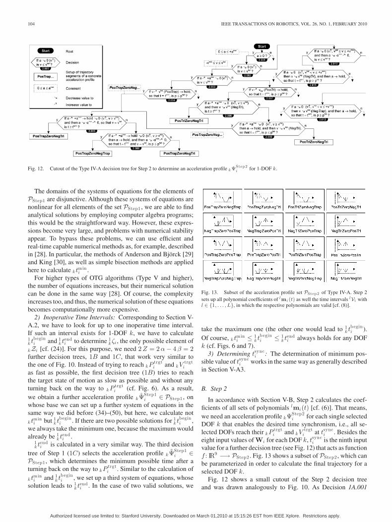
Fig. 12. Cutout of the Type IV-A decision tree for Step 2 to determine an acceleration profile k ΨStep2i for 1-DOF k.

The domains of the systems of equations for the elements ofPStep1 are disjunctive. Although these systems of equations arenonlinear for all elements of the set PStep1 , we are able to findanalytical solutions by employing computer algebra programs;this would be the straightforward way. However, these expres-sions become very large, and problems with numerical stabilityappear. To bypass these problems, we can use efficient andreal-time capable numerical methods as, for example, describedin [28]. In particular, the methods of Anderson and Bjorck [29]and King [30], as well as simple bisection methods are appliedhere to calculate k tmin

i .For higher types of OTG algorithms (Type V and higher),

the number of equations increases, but their numerical solutioncan be done in the same way [28]. Of course, the complexityincreases too, and thus, the numerical solution of these equationsbecomes computationally more expensive.

2) Inoperative Time Intervals: Corresponding to Section V-A.2, we have to look for up to one inoperative time interval.If such an interval exists for 1-DOF k, we have to calculate1k tbegin

i and 1k tend

i to determine 1k ζi , the only possible element of

kZi [cf. (24)]. For this purpose, we need 2Z = 2α − 4β = 2further decision trees, 1B and 1C, that work very similar tothe one of Fig. 10. Instead of trying to reach kP trgt

i and kV trgti

as fast as possible, the first decision tree (1B) tries to reachthe target state of motion as slow as possible and without anyturning back on the way to kP trgt

i (cf. Fig. 6). As a result,we obtain a further acceleration profile k ΨStep1

i ∈ PStep1 , onwhose base we can set up a further system of equations in thesame way we did before (34)–(50), but here, we calculate notk tmin

i but 1k tbegin

i . If there are two possible solutions for 1k tbegin

i ,we always take the minimum one, because the maximum wouldalready be 1

k tendi .

1k tend

i is calculated in a very similar way. The third decisiontree of Step 1 (1C) selects the acceleration profile k ΨStep1

i ∈PStep1 , which determines the minimum possible time after aturning back on the way to kP trgt

i . Similar to the calculation of

k tmini and 1

k tbegini , we set up a third system of equations, whose

solution leads to 1k tend

i . In the case of two valid solutions, we

Fig. 13. Subset of the acceleration profile set PStep2 of Type IV-A. Step 2sets up all polynomial coefficients of lmi (t) as well the time intervals lVi withl ∈ {1, . . . , L}, in which the respective polynomials are valid [cf. (8)].

take the maximum one (the other one would lead to 1k tbegin

i ).Of course, k tmin

i ≤ 1k tbegin

i ≤ 1k tend

i always holds for any DOFk (cf. Figs. 6 and 7).

3) Determining tsynci : The determination of minimum pos-

sible value of tsynci works in the same way as generally described

in Section V-A3.

B. Step 2

In accordance with Section V-B, Step 2 calculates the coef-ficients of all sets of polynomials lmi(t) [cf. (6)]. That means,we need an acceleration profile kΨStep2

i for each single selectedDOF k that enables the desired time synchronism, i.e., all se-lected DOFs reach their kP trgt

i and kV trgti at tsync

i . Besides theeight input values of Wi for each DOF k, tsync

i is the ninth inputvalue for a further decision tree (see Fig. 12) that acts as functionf : IR9 −→ PStep2 . Fig. 13 shows a subset of PStep2 , which canbe parameterized in order to calculate the final trajectory for aselected DOF k.

Fig. 12 shows a small cutout of the Step 2 decision treeand was drawn analogously to Fig. 10. As Decision 1A.001



Fig. 14. PosTriZeroNegTri profile with all relevant variables such that a systemof equations can be set up and solved in order to calculate kMi for 1-DOF k.

does, Decision 2.001 checks whether the current accelerationvalue kAi is positive or negative. We assume to take the leftbranch, and let Decision 2.002 check whether the velocityvalue would be greater or less then k vtrgt

i after −kJmaxi has

been applied to decrease the acceleration value to zero. De-cision 2.003 checks whether kAmax

i must be applied to reachk vtrgt

i , i.e., we find out whether a positive triangle or trape-zoidal acceleration profile would lead us to k vtrgt

i . We as-sume that a trapezoidal profile is required. Decision 2.004 in-spects whether the resulting position value of DOF k at tsync

i

is greater or less than kptrgti if kvtrgt

i would be reached assoon as possible by applying a trapezoidal acceleration pro-file (PosTrap). If the resulting value is less, we know that wewill have to increase the hold time of the trapezoidal accelera-tion profile, i.e., a PosTrapZeroNeg. . . profile will be required.Before we decide whether kΨStep2

i = PosTrapZeroNegTri or

kΨStep2i = PosTrapZeroNegTrap is correct, Decision 2.005 ver-

ifies whether we would have enough time to apply a positivetrapezoidal acceleration profile directly followed by a negativetriangle-shaped profile that exactly touches −kAmax

i such thatk vtrgt

i is finally reached. If we do not have enough time for thisacceleration progression, kΨStep2

i = PosTrapZeroNegTri willbe the solution. If there is enough time for the accelerationbehavior checked by Decision 2.005, Decision 2.006 will checkthe boundary case for the profiles PosTrapZeroNegTrap and Pos-TrapZeroNegTri and finally determine the acceleration profile.The decisions from 2.007 to 2.012 work analogously.

Analogous to the system of equations given by (34)–(50), wecan set up a further system of equations for each kΨStep2

i ∈PStep2 (cf. Fig. 13), whose solution delivers all required pa-rameters for all L trajectory segments lmi ∀ l ∈ {1, . . . , L}[cf. (7)] as well as all time intervals lVi [cf. (8)]. This pro-cedure will be exemplarily explained by means of the profilesΨStep2 = PosTriZeroNegTri, as shown in Fig. 14 (cf. top rightelement of Fig. 13). In a straightforward way, we can set up asystem of 14 equations for each selected DOF k at time instant Ti

2k ti − Ti =

(kapeak1 − kAi)kJmax

i

(51)

3k ti − 2

k ti = kapeak1

kJmaxi

(52)

5k ti − 4

k ti = − kapeak2

kJmaxi

(53)

tsynci − 5

k ti = − kapeak2

kJmaxi

(54)

2kvi − Vi =

12(2k ti − Ti

)(kAi + kapeak1) (55)

3k vi − 2

kvi =12(3k ti − 2

k ti)kapeak1 (56)

4k vi − 3

kvi = 0 (57)

5k vi − 4

kvi =12(5k ti − 4

k ti)kapeak2 (58)

kV trgti − 5

kvi =12(tsynci − 5

k ti)kapeak2 (59)

2kpi − kPi = kVi

(2k ti − Ti

)+

12 kAi

(2k ti − Ti

)2

+16 kJmax

i

(2k ti − Ti

)3(60)

3kpi − 2

kpi = 2k vi

(3k ti − 2

k ti)

+12 kapeak1

i

(3k ti − 2

k ti)2

− 16 k

Jmaxi

(3k ti − 2

k ti)3

(61)

4kpi − 3

kpi = 3k vi

(4k ti − 3

k ti)

(62)

5kpi − 4

kpi = 4k vi

(5k ti − 4

k ti)− 1

6 kJmaxi

(5k ti − 4

k ti)3

(63)

kP trgti − 5

kpi = 5k vi

(tsynci − 5

k ti)

+12 kapeak2

i

(tsynci − 5

k ti)2

+16 kJmax

i

(tsynci − 5

k ti)3

. (64)

There is a significant difference between the systems ofequations for Step 1 (34)–(50) and Step 2 (51)–(64). In Step 1,there is a number of systems of equations (elements of PStep1),which lead to a valid solution, but in Step 2, exactly one systemof equations sΨStep2 leads to the desired solution. This systemhas to be determined by the decision tree of Fig. 12.

The solution of (51)–(64) contains 2k ti , 3

k ti , 4k ti , 5

k ti , 2kvi , 3

kvi ,4kvi , 5

k vi , 2kpi , 3

kpi , 4kpi , 5

kpi , kapeak1i , and kapeak2

i . The first fourvalues of this list together with Ti and tsync

i compose lkϑi ∀ l ∈

{1, . . . , 5} [cf. (8)]. The latter eight values are used to calculatethe motion polynomials at time instant Ti

lk �mi ∀ l ∈ {1, . . . , 5}

such that the trajectory for DOF k kMi is completely described.

C. Step 3

Step 3 calculates the output values �Pi+1 , �Vi+1 , and �Ai+1 andworks according to Section V-C.

D. Final Remarks on the Type IV-A OTG Algorithm

Because these decision trees would take too much space, theycannot be depicted completely in a book, thesis, or paper. Thefollowing gives an impression of the complexity: The tree 1B—written in font size of 10 pt, prepared in a minimized version,



TABLE IINUMBER OF NODES PER DECISION TREE FOR THE TYPE IV,

VARIANT A OTG ALGORITHM

and with all nodes tightly arranged—can just be plotted on aposter of DIN A0 size. Even the description would fill a book ofseveral hundred pages such that here only an impression shallbe imparted, and only the basic conceptual ideas are explained.The cutouts of the two Type IV decision trees presented in Figs.10 and 12 can only be considered as small samples. The totalnumbers of nodes per tree for the Type IV-A OTG algorithm aregiven by Table II. Minimized means that the number of nodeswas minimized, i.e., subtrees were used multiple times (e.g., inthe tree of Fig. 12, the decisions 2.005 and 2.006 are used twicein order to save space; although this kind of representation lookslike a graph, the actual structure is a tree, i.e., there are no loopsexistent).

The challenge during the development of decision trees isthe guarantee that (22) and (30) hold. When starting to developa decision tree, the motion profile sets PStep1 and PStep2 areunknown [cf. (20) and (25)]. These two sets have to fit exactlyto each other such that the two equations mentioned above hold.The design of these sets can only take place during the devel-opment of the (2α − 4β) (cf. Table I) decision trees, becausewe cannot know how these profiles look like until we know allpossible cases. Summarizing this

1) if we knew the motion profile sets PStep1 and PStep2 (andthus, all input domains rDStep1 ∀ r ∈ {1, . . . , R} andsDStep2 ∀ s ∈ {1, . . . , S}) for a concrete type of OTG, itmight be possible to generate the decision trees automati-cally;

2) if we knew all (2α − 4β) decision trees for a concretetype of OTG, it would be possible to determine the motionprofile sets PStep1 and PStep2 .

However, since we neither know PStep1 or PStep2 of a con-crete type nor the decision trees beforehand, it cannot be possibleto generate an OTG algorithm automatically. For the validationof (20), (22), (25), and (30), random input values Wi are gen-erated until every single edge of the trees (and thus, also everysingle profile of the sets PStep1 and PStep2 , cf. Table II) wereused at least once.

VII. RELATION TO HIGH-LEVEL MOTION-PLANNING SYSTEMS

Robot motion planning and, in particular, path planning be-long to the classic and fundamental areas of robotics. Here, weregard a special field of this area: real-time adaptive motionplanning (RAMP, [10]). We assume robots that have to act in adynamic and/or unknown environment and which are equippedwith sensor systems to react to (unknown) static or dynamicobstacles, events, or abrupt changes of task parameters. Refer-ences [11] and [31] give general overviews about the field of

Fig. 15. High-level motion planning system may calculate intermediate mo-tion states h Mtrgt

0 ∀ h ∈ {1, . . . , 7} in configuration space, which are passed

through by the online-generated trajectories from �P0 to �P trgt0 .

motion planning, and [10], [32], and [33] focus on real-timecapable methods for (multi-)robot motion planning.

As in [10], the generation of splines is one commonly usedmethod to represent calculated trajectories; it is the task of amotion-planning algorithm to calculate respective knots. In [33],collision-free vertices (“milestones”) and edges on a roadmap,which is another kind of representation, are used to representcurrently planned trajectories. These knots or milestones aregenerated from an overall view onto the robotic system and itsenvironment—it is, in particular, a kind of motion planning froma global point of view. The output values of such higher levelmotion-planning systems, i.e., the knots and milestones, can beideally used as input values for the OTG algorithm such that thecombination of these systems leads to a very good symbiosis.Based on this idea, we can realize robotic systems which canmove according to global and task-dependent motion planningand do not loose the ability to instantaneously react to low-levelsensor events.

This is also comparable to human scenarios: If we unex-pectedly touch a very spiky object and suddenly perceive pain,we can immediately pull our hand away in a reactive manner(without thinking, i.e., without global motion planning). As con-sequence, the OTG would be responsible for providing a kindof robot reflex, as was discussed in Section II.

In the following, we explain this idea by means of a concrete,simple, and static example. For illustration, Fig. 15 depicts aconfiguration space obstacle in 2-D-dimensional space. The taskof the robot is to move from �P0 = (50, 50)mm to �P trgt

0 =(700, 300)mm. For this purpose, the high-level motion planningsystem may calculate intermediate motion states

hMtrgt0 =

(h �P trgt0 , h �V trgt

0 , h �Atrgt0

), with h ∈ {1, . . . , H}

(65)

which have to be passed through by the trajectories of the OTGalgorithm. H is the number of calculated motion states, whichcorrespond to the knots [10] or milestones [33], i.e., the mo-tion states of (65) constitute the interface to the high-level



Fig. 16. Complete decision tree to determine the acceleration profile for trans-ferring the target state of motion h Mtrgt

0 to zero velocity and zero accelerationin a time-optimal way as it would be required for the OTG algorithms ofTypes IV and V.

motion-planning system. Of course, hBi [cf. (3)] can also beadapted for the motions in-between two knots. In the case ofdynamic environments, all motion states, which have not beenpassed by the robot yet, can, of course, be furthermore adaptedat any future time.

The result of Fig. 15 was achieved with the Type IV-B OTGalgorithm, i.e., h �Atrgt

0 = �0 ∀ h ∈ {1, . . . , 7} such that velocityvectors were simply put into the given configuration space

1 �P trgt0 = (300, 100)mm 1 �V trgt

0 = (80, 30) mm/s

2 �P trgt0 = (500, 300)mm 2 �V trgt

0 = (−30, 100) mm/s

3 �P trgt0 = (400, 450)mm 3 �V trgt

0 = (−10, 100) mm/s

4 �P trgt0 = (400, 600)mm 4 �V trgt

0 = (−50, 80) mm/s

5 �P trgt0 = (500, 800)mm 5 �V trgt

0 = (60, 40) mm/s

6 �P trgt0 = (650, 850)mm 6 �V trgt

0 = (120, 0) mm/s

7 �P trgt0 = (800, 800)mm 7 �V trgt

0 = (150,−70) mm/s.

Finally, �P trgt0 = (700, 300) mm is achieved with zero velocity.

Depending on the type of OTG, several restrictions mayhold for the higher level planning algorithms. As discussedin Section IV-C, (18) only holds for the Types I, III, and VI.To keep the position of the system within its positional limits(k

�Pmini , k

�Pmaxi ), we have to assure the target states of motion

hMtrgti ∀ h ∈ {1, . . . , H} are bounded. Analogous to the de-

cision trees of Figs. 10 and 12, Fig. 16 depicts the completedecision tree used for the calculation of the the actual val-ues of h �P trgt

i in hMtrgti for the OTG Types IV and V. First,

one out of four acceleration profiles is determined to transferhMtrgt

i to zero velocity and zero acceleration in a time-optimalway.

In the same way the systems of equations in (34)–(50) and(51)–(64) were set up based on the acceleration profiles of

Fig. 17. Sample of a Type IV trajectory for K = 4 DOFs.

Figs. 11 and 14, the value for the required position differ-ence (i.e., the minimum distance between kPmin

i or kPmaxi and

hk P trgt

i ) can be calculated in a closed form for each of the fouracceleration profiles of Fig. 16.

This section introduced how an OTG algorithm can act as aninterface to higher level motion planning systems. The majorsymbiotic effect of this use case is that a robotic system, whichis guided by a higher level planning system, can obtain theability of performing immediate reflex motions as instantaneousreactions to unforeseen events.

VIII. RESULTS OF TYPE IV ONLINE TRAJECTORY GENERATION

A. Handling Arbitrary States of Motion

Earlier, we have only discussed the mathematical basics forType IV OTG. To clarify the idea of this paper, Fig. 17 exem-plarily illustrates one concrete result trajectory for K = 4 DOFs,i.e., the Type IV OTG acts as function f : IR32 × IB4 −→ IR12 ,which is computed every control cycle. Our implemented robotmotion controller works at a frequency of 1 KHz such that thealgorithm is called once per T cycle = 1 ms. The given arbitrary



Fig. 18. XY plot of the exemplary geometric of a 2-DOF path according thetrajectory in Fig. 19 with and without sensor event.

motion parameters are (normalized values, without units):

�P0 = (100,−200, 400,−800)T

�V0 = (300,−200,−50, 200)T

�A0 = (−350,−300,−50, 350)T

M0

�P trgt0 = (−800,−500,−300,−400)T

�V trgt0 = (−50,−50,−100,−400)T

}

Mtrgt0

�V max0 = (800, 750, 150, 600)T

�Amax0 = (400, 400, 100, 300)T

�Jmax0 = (200, 400, 100, 600)T

B0

�S0 = (1, 1, 1, 1)T

W0 .

In Fig. 17, one can clearly recognize that all four DOFs reachtheir desired state of motion Mtrgt

i at the same time instanttsynci = 5340ms ∀ i ∈ {0, . . . , 5340} (N = 5340 cycles, i.e.,

the OTG algorithm was executed 5340 times). tsynci was deter-

mined by 3tmini . The selected acceleration profiles are

1ΨStep2i = NegTrapZeroPosTri

2ΨStep2i = PosTriZeroNegTri

3ΨStep2i = NegTrapZeroPosTri

4ΨStep2i = NegTriZeroNegTrap.

For simplicity, the input parameters Mtrgti , Bi , and �Si

remained constant during the whole execution time fromT0 to TN , i.e., Mtrgt

i = Mtrgt0 ∧ Bi = B0 ∧ �Si = �S0 ∀ i ∈

{0, . . . , 5340} [cf. (1) and (10)].

B. Reaction to Sensor Events

This section explains, how the OTG is applied to the simplestcase of sensor-guarded motion control. For a simple and cleardemonstration, we consider only a 2-DOF Cartesian robot. Ofcourse, the OTG concept works for any number of DOFs K.

Fig. 18 depicts the geometric path of a trivial point-to-pointmotion (dotted line). It is the robot’s task to move from aninitial position �P0 to a target position �P trgt

0 under the kinematic

Fig. 19. Position, velocity, and acceleration progressions of the 2-DOF TypeIV-A trajectory that corresponds to the path of Fig. 18.

constraints of �V max0 , �Amax

0 , and �Jmax0

�P0 = (100, 200)T mm

�P trgt0 = (800, 850)T mm

�V max0 = (300, 200)T mm/s

�Amax0 = (200, 300)T mm/s2

�Jmax0 = (400, 500)T mm/s3 .

In the following, we analyze this for two cases.1) Without Obstacle: If we would not have to react to sen-

sor events, off-line methods, which belong to the most classicones in the field of robot-motion control, could be applied. Anoverview of trajectory generation methods is given in [27]. Theresulting path is marked by the dotted line. The position, ve-locity, and acceleration progressions of the original trajectoryare also depicted in Fig. 19 (dash-dotted and dotted lines). Ascan be seen in the bottom diagram of Fig. 19, both DOFs aretransferred into their target positions by trapezoidal accelerationprofiles such that both reach their target state at t = 4518 mswith symmetrical velocity profiles.

2) With Obstacle and Reaction to Sensor Event: If we con-sider unknown objects/obstacles in our workspace, we have toreact right after their detection. The results of this procedureare illustrated by the solid line in Fig. 18 and the solid and



dashed lines of the diagrams in Fig. 19. Type IV-A OTG is ap-plied in this example. Due to some sensor, the system detectsthe unforeseen obstacle at t = 1674 ms (1P1674 = 300 mm, cf.Figs. 18 and 19). A simple solution could then be the abruptchange of the target position values in the moment of obstacledetection, for example, to �P trgt

1674 = (800, 600)T mm, such thatwe would prevent the collision with the object. After reaching�P trgt

1674 , the old target position �P trgt0 could then be reused to reach

the originally desired position.See the velocity and acceleration progressions in Fig. 19.

Compared to the earlier idea, we present an advanced andmore dynamic version in which the system puts an intermediatetarget-velocity vector �V trgt

1674 = (100, 100)T mm/s into the posi-tion �P trgt

1674 = (800, 600)T mm in order to bypass the obstacle dy-namically. Right after �P trgt

1674 and �V trgt1674 have been time-optimally

reached (at t = 3879 ms, cf. Fig. 19), a second (abrupt) switch-ing of input parameters occurs, and the system sets up the origi-nal parameters again ( �P trgt

3879 = �P trgt0 and �V trgt

3879 = �0). These arefinally reached at t = 6 s (cf. Fig. 19).

Final Remarks : The OTG algorithm is executed every mil-lisecond, and the output values of the algorithm lead to con-tinuous trajectories, which reach each desired state of motiontime optimally and time-synchronized. Furthermore, all kine-matic motion constraints, �V max

0 , �Amax0 , and �Jmax

0 are kept dur-ing the whole trajectory. How the intermediate positions andvelocity vectors as �P trgt

1674 and �V trgt1674 are calculated depends on

the system layer above the OTG (cf. Section VII).

C. Switching From Sensor-Guided Motion Controlto Trajectory-Following Control

This paper contains theory, simulation results, and real-worldexperimental results. The latter demonstrates the functionalityof the OTG concept in practice and is presented in this section.For the experiments, the following hardware setup has beenused: The original controller of a Staubli RX60 industrial ma-nipulator [34] was replaced, and the frequency inverters weredirectly interfaced. Three PCs running with QNX [35] as real-time operating system perform a control rate of 10 kHz for thejoint controllers; a hybrid switched-system controller is used forCartesian space control and runs at a frequency of 1 kHz.

To explain the behavior of instantaneous switchings fromsensor-guided control to trajectory-following control, Fig. 20now closes the loop of the introductory chapter (cf. Fig. 1). AtT0 = 0ms, a sensor-guided robot motion command was exe-cuted w.r.t. the hand frame of the manipulator. All six Carte-sian DOFs are controlled by a simple zero-force/torque con-troller (proportional-integral differential), which uses unfilteredforce/torque values of a JR3 force/torque sensor [36].2 This wasdone intentionally in order to show the response of the overallsystem (including the OTG algorithm) on strongly noised sen-sor data. At t = 586ms, a (sensor) event happens, and the sys-tem instantaneously switches from sensor-guided robot-motioncontrol to trajectory-following control. The new trajectory iscalculated instantaneously (within the control cycle after the

2Sensor model 85M35A-40 200N12, receiver board running at 8 kHz.

Fig. 20. Position, velocity, and acceleration progressions in Cartesian spaceof a sample motion of Staubli RX60 industrial manipulator. First, all six DOFsare controlled by a feedback controller using force/torque sensor signals. Att = 584 ms, an event happens, and the (open-loop) Type IV OTG algorithmtakes over control.

event) and the manipulator performs a smooth, continuous mo-tion. Here, this is done for all six DOFs, i.e., the selectionvector switches from �S585 = �0 to �S586 = �1. Of course, it wouldalso be possible that only some DOFs were switched from onecontroller to another. To describe the relevance for industrialpractice, imagine that a sensor (e.g., a force/torque sensor or avision system) fails during a sensor-guided robot motion, andthen, the OTG algorithm can always take over control in anystate of motion and at any time such that a smooth, continuousmotion results. Furthermore, if a desired (force/torque or vision)set-point cannot be achieved for some reason, the current motioncan be interrupted at any instant such that the OTG algorithmguides respective DOFs to a safe state.



The computations for this 6-DOF system requires an aver-age execution time of 135µs on a single-core machine.3 Theworst-case execution time is 540µs. This difference is due tothe calculation of inoperative time intervals. In most cases, in-operative time intervals are not existent, but for the worst case,they are considered for all DOFs.

IX. CONCLUSION AND OUTLOOK

This work introduced a new concept for motion generation inrobotic systems during runtime. The presented online trajectory-generation algorithm is executed in parallel to low-level motioncontrollers such that systems using it are able to react instan-taneously to unforeseen (sensor) events. In particular, the algo-rithm closes a significant gap: Switching from sensor-guidedmachine motions to trajectory-following motions becomes pos-sible at any time and in any state of motion. As a consequence,(multi)sensor integration becomes substantially simplified, androbot-motion control systems are enabled to execute trajectory-following motions, sensor-guided motions, and sensor-guardedmotions within one framework. The proposed online trajectory-generation algorithm acts as an open-loop controller and cantake over control at any time instant such that safe and continu-ous motions can be guaranteed—even if sensors fail.

The algorithm was developed with the aim to advance mo-tion control systems for many robotic applications in variousfields, such as service robotics, manipulation control systems,mobile robotics and manipulation, or robotic surgery—in short,all fields in which sensor integration plays a fundamental role.The algorithm can be regarded as an intermediate control layer,thus constituting one element of the important bridge betweenlow-level robot motion control and higher level (sensor-based)motion planning.

Besides the general theory of online trajectory generation,this contribution introduced the A-variants of OTG, i.e., thekinematic-motion constraint values for velocity, acceleration,jerk, and derivative of jerk remain constant. In a follow-up pub-lication, we will present the procedures and results of the B-variants (i.e., the matrix Bi becomes time-variant), which arerequired for the embedding of robot dynamics, for unforeseencontrol-space switchings, and for unforeseen reference-frameswitchings. Furthermore, an adaptation of the algorithm will bedescribed that enables the generation of homothetic trajectories(i.e., straight-line trajectories).

ACKNOWLEDGMENT

The authors wish to thank the anonymous reviewers for theirinvaluable comments, which helped us to improve the qual-ity of this paper. The works of our former diploma studentsM. Hanisch, C. Hurnaus, and A. Tomiczek, who worked hardon the first ideas and implementations of this concept, are highlyappreciated. Furthermore, the authors would like to thank QNXSoftware Systems for providing free software licenses for exper-imental setups.

3Used hardware: AMD Athlon64 3700+ (2.2 GHz, 1024 KB L2 Cache),2-GB DDR-400, gigabyte GA-K8NF9 ultra F5 mainboard.

REFERENCES

[1] B. Siciliano and L. Villani, Robot Force Control. Norwell, MA: Kluwer,1999.

[2] F. Chaumentte and S. A. Hutchinson, “Visual servoing and visual track-ing,” in Springer Handbook of Robotics, 1st ed., B. Siciliano and O. Khatib,Eds. Berlin, Germany: Springer-Verlag, 2008 ch. 24, pp. 563–583.

[3] T. Kroger, B. Finkemeyer, S. Winkelbach, S. Molkenstruck, L.-O. Eble,and F. M. Wahl, “A manipulator plays Jenga,” IEEE Robot. Autom. Mag.,vol. 15, no. 3, pp. 79–84, Sep. 2008.

[4] Hasbro, Inc. (2008). Jenga homepage. [Online]. Pawtucket, RI. Available:http://www.jenga.com

[5] M. E. Kahn and B. Roth, “The near-minimum-time control of open-looparticulated kinematic chains,” ASME J. Dyn. Syst., Meas., Control, vol. 93,pp. 164–172, Sep. 1971.

[6] M. Brady, “Trajectory planning,” in Robot Motion: Planning and Control,M. Brady, J. M. Hollerbach, T. L. Johnson, T. Lozano-Perez, and M.T. Mason, Eds. Cambridge, MA: MIT Press, 1982, ch. 4, pp. 221–243.

[7] J. E. Bobrow, S. Dubowsky, and J. S. Gibson, “Time-optimal control ofrobotic manipulators along specified paths,” Int. J. Robot. Res., vol. 4,no. 3, pp. 3–17, Fall 1985.

[8] K. J. Kyriakopoulos and G. N. Sridis, “Minimum jerk path generation,” inProc. IEEE Int. Conf. Robot. Autom., Philadelphia, PA, Apr. 1988, vol. 1,pp. 364–369.

[9] P. Lambrechts, M. Boerlage, and M. Steinbuch, “Trajectory planning andfeedforward design for high performance motion systems,” in Proc. Amer.Control Conf., Boston, MA, Jun. 2004, vol. 5, pp. 4637–4642.

[10] J. Vannoy and J. Xiao, “Real-time adaptive motion planning (RAMP) ofmobile manipulators in dynamic environments with unforeseen changes,”IEEE Trans. Robot., vol. 24, no. 5, pp. 1199–1212, Oct. 2008.

[11] S. Lindemann and S. LaValle, “Current issues in sampling-based motionplanning,” in Proc. 8th Int. Symp. Robot. Res., P. Dario and R. Chatila,Eds. Berlin, Germany: Springer-Verlag, 2004, pp. 36–54.

[12] O. Brock and O. Khatib, “Elastic strips: A framework for motion gen-eration in human environments,” Int. J. Robot. Res., vol. 21, no. 12,pp. 1031–1052, Dec. 2002.

[13] O. Brock, J. Kuffner, and J. Xiao, “Manipulation for robot tasks,” inSpringer Handbook of Robotics, 1st ed., B. Siciliano and O. Khatib, Eds.Berlin, Germany: Springer-Verlag, 2008, ch. 26, pp. 615–645.

[14] S. Macfarlane and E. A. Croft, “Jerk-bounded manipulator trajectory plan-ning: Design for real-time applications,” IEEE Trans. Robot. Autom.,vol. 19, no. 1, pp. 42–52, Feb. 2003.

[15] B. Cao, G. I. Dodds, and G. W. Irwin, “A practical approach to neartime-optimal inspection-task-sequence planning for two cooperative in-dustrial robot arms,” Int. J. Robot. Res., vol. 17, no. 8, pp. 858–867, Aug.1998.

[16] X. Broquere, D. Sidobre, and I. Herrera-Aguilar, “Soft motion trajectoryplanner for service manipulator robot,” in Proc. IEEE/RSJ Int. Conf. Intell.Robots Syst., Nice, France, Sep. 2008, pp. 2808–2813.

[17] S. Liu, “An on-line reference-trajectory generator for smooth motion ofimpulse-controlled industrial manipulators,” in Proc. 7th Int. WorkshopAdv. Motion Control, Maribor, Slovenia, Jul. 2002, pp. 365–370.

[18] R. Haschke, E. Weitnauer, and H. Ritter, “On-line planning of time-optimal, jerk-limited trajectories,” in Proc. IEEE/RSJ Int. Conf. Intell.Robots Syst., Nice, France, Sep. 2008, pp. 3248–3253.

[19] K. Ahn, W. K. Chung, and Y. Yourn, “Arbitrary states polynomial-liketrajectory (ASPOT) generation,” in Proc. 30th Annu. Conf. IEEE Ind.Electron. Soc., Busan, Korea, Nov. 2004, vol. 1, pp. 123–128.

[20] R. H. Castain and R. P. Paul, “An on-line dynamic trajectory generator,”Int. J. Robot. Res., vol. 3, no. 1, pp. 68–72, Mar. 1984.

[21] J. Heinzmann and A. Zelinsky, “Quantitative safety guarantees for phys-ical human–robot interaction,” Int. J. Robot. Res., vol. 22, no. nos. 7/8,pp. 479–504, Jul. 2003.

[22] A. D. Santis, A. Albu-Schaffer, C. Ott, B. Siciliano, and G. Hirzinger,“The skeleton algorithm for self-collision avoidance of a humanoid ma-nipulator,” in Proc. IEEE/ASME Int. Conf. Adv. Intell. Mechatron., Zurich,Switzerland, Sep. 2007, pp. 1–6.

[23] A. D. Santis and B. Siciliano, “Reactive collision avoidance for saferhuman–robot interaction,” presented at the IARP IEEE/RAS-EURONWorkshop Tech. Challenges Dependable Robots Hum. Environ., Roma,Italy, Apr. 2007.

[24] S. Haddadin, A. Albu-Schaffer, A. D. Luca, and G. Hirzinger, “Collisiondetection and reaction: A contribution to safe physical human–robot in-teraction,” in Proc. IEEE/RSJ Int. Conf. Intell. Robots Syst., Nice, France,Sep. 2008, pp. 3356–3363.



[25] A. Albu-Schaffer and C.Ott, G. Hirzinger, “A unified passivity-basedcontrol framework for position, torque and impedance control of flexiblejoint robots,” Int. J. Robot. Res., vol. 26, no. 1, pp. 23–39, Jan. 2007.

[26] T. Kroger, A. Tomiczek, and F. M. Wahl, “Towards on-line trajectorycomputation,” in Proc. IEEE/RSJ Int. Conf. Intell. Robots Syst., Beijing,China, Oct. 2006, pp. 736–741.

[27] W. Khalil and E. Dombre, Modeling, Identification and Control of Robots,Trajectory Generation, 1st ed. London, U.K.: Hermes Penton, 2002, ch.13, pp. 313–345.

[28] G. Engeln-Mullges and F. Uhlig, Numerical Algorithms with C. NewYork: Springer-Verlag, 1996.

[29] N. Anderson and A. Bjorck, “A new high order method of regula falsitype for computing a root of an equation,” BIT Numer. Math., vol. 13,no. 3, pp. 253–264, Sep. 1973.

[30] R. King, “An improved pegasus method for root finding,” BIT Numer.Math., vol. 13, no. 4, pp. 423–427, Dec. 1973.

[31] H. H. Gonzalez-Banos, D. Hsu, and J.-C. Latombe, “Motion planning:Recent developments,” in Autonomous Mobile Robots: Sensing, Control,Decision-Making and Applications, S. S. Ge and F. L. Lewis, Eds. BocaRaton, FL: CRC, 2006, ch. 10.

[32] O. Brock and L. E. Kavraki, “Decomposition-based motion planning: Aframework for real-time motion planning in high-dimensional configura-tion spaces,” in Proc. IEEE Int. Conf. Robot. Autom., Seoul, Korea, May2001, pp. 1469–1474.

[33] Y. Yang and O. Brock, “Elastic roadmaps: Globally task-consistent mo-tion for autonomous mobile manipulation in dynamic environments,” pre-sented at the Robot.: Sci. Syst. Conf., Philadelphia, PA, Aug. 2006.

[34] Staubli Faverges SCA. (2008), Faverges (Annecy), France. [Online].Available: http://www.staubli.com/en/robotics

[35] QNX Software Systems. (2008). Ottawa, ON, Canada. [Online].Available: http://www.qnx.com

[36] JR3, Inc. (2008). Woodland, CA. [Online]. Available: http://www.jr3.com

Torsten Kroger (M’02) received the Ph.D. de-gree from the Institut fur Robotik und Prozessinfor-matik, Technische Universitat Carolo-Wilhelmina zuBraunschweig, Braunschweig, Germany, in 2009.

In 2001, he attended an industrial internship atLenze Corporation, Atlanta, GA. He finished hisstudies in electrical engineering at the TechnischeUniversitat Carolo-Wilhelmina zu Braunschweig in2002. Since 2003, he has been a Research Fellowwith the Institut fur Robotik und Prozessinformatik,Technische Universitat Carolo-Wilhelmina zu Braun-

schweig. Since 2006, he has been a Technical Consulter for several companiesdealing with robot technologies. His current research interests include onlinetrajectory generation, hybrid switched-motion control, multisensor integration,and new robot-programming paradigms.

Friedrich M. Wahl (M’82) studied electrical en-gineering/cybernetics at the Technical University ofMunich, Munich, Germany, from which he receivedthe Diploma, Ph.D., and “venia legendi” degrees indigital signal and image processing in 1974, 1980,and 1984, respectively.

From 1974 to 1981, he conducted research withthe Institute of Communication Engineering, Tech-nical University of Munich, in the fields of patternrecognition and signal and image processing. From1981 to 1986, he was with the IBM Research Lab-

oratories, San Jose, CA, and Zurich, Switzerland, where he was enagaged inresearch in the areas of document analysis, industrial image analysis, and ma-chine vision. Since 1986, he has been a Professor of computer science with theTechnische Universitat Carolo-Wilhelmina zu Braunschweig, Braunschweig,Germany, where he set up the Institut fur Robotik und Prozessinformatik. Hebecame an Advisory Professor with Shanghai University, Shanghai, China, in1992 and Chairman of the Collaborative Research Centre on Robotic Systemsfor handling and assembly with the Technische Universitat Carolo-Wilhelminazu Braunschweig in 2000. His current research interests include robotics, com-puter vision, and algorithmic aspects of computer science.


94 ieee transactions on robotics, vol. 26, no. 1, …96 ieee transactions on robotics, vol. 26, no....

Documents