9/24/2013phy 113 c fall 2013-- lecture 91 phy 113 c general physics i 11 am-12:15 pm mwf olin 101...
TRANSCRIPT

PHY 113 C Fall 2013-- Lecture 9 19/24/2013
PHY 113 C General Physics I11 AM-12:15 PM MWF Olin 101
Plan for Lecture 9:
1. Review (Chapters 1-8)
2. Exam preparation advice –
3. Example problems

PHY 113 C Fall 2013-- Lecture 9 29/24/2013

PHY 113 C Fall 2013-- Lecture 9 39/24/2013
iclicker questionWhat is the best way to prepare for Thursday’s exam?
A. Read Lecture Notes and also reread Chapters 1-8 in Serway and Jewett.
B. Prepare equation sheet.C. Solve problems from previous exams.D. Solve homework assignments (both graded and
ungraded) from Webassign Assignments 1-8E. All the above

PHY 113 C Fall 2013-- Lecture 9 49/24/2013
iclicker questionHave you (yet) accessed the online class lecture notes from previous classes?
A. yesB. no
iclicker questionHave you (yet) accessed the passed Webassign Assignments (with or without the answer key)?
C. yesD. no

PHY 113 C Fall 2013-- Lecture 9 59/24/2013
Access to previous exams

PHY 113 C Fall 2013-- Lecture 9 69/24/2013
Previous exam access -- continued
Overlap with 2013 schedule

PHY 113 C Fall 2013-- Lecture 9 79/24/2013
Comments on preparation for next Thursday’s exam – continued
What you should bring to the exam (in addition to your well-rested brain): A pencil or pen Your calculator An 8.5”x11” sheet of paper with your favorite
equations (to be turned in together with the exam)
What you should NOT use during the exam Electronic devices (cell phone, laptop, etc.) Your textbook

PHY 113 C Fall 2013-- Lecture 9 8
Advice:
1. Keep basic concepts and equations at the top of your head.
2. Practice problem solving and math skills
3. Develop an equation sheet that you can consult.
Equation Sheet
dt
ddt
d
m
rv
va
aF
Problem solving skills
Math skills
9/24/2013

PHY 113 C Fall 2013-- Lecture 9 99/24/2013
iclicker exerciseDoes the previous slide annoy you?
A. yesB. no

PHY 113 C Fall 2013-- Lecture 9 10
Problem solving steps
1. Visualize problem – labeling variables2. Determine which basic physical principle(s) apply3. Write down the appropriate equations using the variables
defined in step 1.4. Check whether you have the correct amount of
information to solve the problem (same number of knowns and unknowns).
5. Solve the equations.6. Check whether your answer makes sense (units, order of
magnitude, etc.).
9/24/2013

PHY 113 C Fall 2013-- Lecture 9 119/24/2013
Likely exam format (example from previous exam)

PHY 113 C Fall 2013-- Lecture 9 129/24/2013
Likely exam format (example from previous exam)
PHY 113 C Fall 2013-- Lecture 9 139/24/2013
Review of slides from previous lectures

PHY 113 C Fall 2013-- Lecture 9 149/24/2013
Mathematics Review -- Appendix B Serwey & Jewett
a
acbbx
cbxax
2
4
0
:equation Quadratic
2
2
)cos()sin(
:calculus alDifferenti
1
ttdt
d
eedt
d
antatdt
d
tt
nn
)cos(1
)sin(
11
:calculus Integral1
tdtt
edte
n
atdtat
tt
nn
a
b
c
q
b
ac
ac
b
tan
sin
cos
:ryTrigonomet

PHY 113 C Fall 2013-- Lecture 9 159/24/2013
One dimensional motion --Summary of relationships
t
t
t
t
dttatvdt
dvta
dttvtxdt
dxtv
0
0
')'()( )(
')'()( )(

PHY 113 C Fall 2013-- Lecture 9 169/24/2013
Special relationships between t,x,v,a for constant a:
t
t
t
t
dttatvdt
dvta
dttvtxdt
dxtv
0
0
')'()( )(
')'()( )(
:iprelationsh General
200
2
0
2
1
2
100)(
0)(
:iprelationsh Special
attvxattvxtx
atvatvtv

PHY 113 C Fall 2013-- Lecture 9 179/24/2013
Vector addition:
ab
a – b
Vector subtraction:
a
-b
a + bIntroduction of vectors

PHY 113 C Fall 2013-- Lecture 9 189/24/2013
ax
ay
22
ˆˆ
ˆˆ and ˆˆFor
yx
yyxx
yxyx
cc
baba
bbaa
c
cyxba
yxbyxa
yxa ˆˆ yx aa
by
bx
yxb ˆˆ yx bb cba
Treatment of vectors in component form

PHY 113 C Fall 2013-- Lecture 9 199/24/2013
Vectors relevant to motion in two dimenstions
Displacement: r(t) = x(t) i + y(t) j
Velocity: v(t) = vx(t) i + vy(t) j
Acceleration: a(t) = ax(t) i + ay(t) j
dtdx
x vdtdy
y v
dt
dvxx a
dt
dvyy a

PHY 113 C Fall 2013-- Lecture 9 209/24/2013
Visualization of the position vector r(t) of a particle
r(t1)r(t2)

PHY 113 C Fall 2013-- Lecture 9 219/24/2013
Visualization of the velocity vector v(t) of a particle
r(t1)
r(t2)
12
12
0
)()(lim
12 tt
tt
dt
dt
tt
rrrv
v(t)

PHY 113 C Fall 2013-- Lecture 9 229/24/2013
Visualization of the acceleration vector a(t) of a particle
r(t1)
r(t2)
12
12
0
)()(lim
12 tt
tt
dt
dt
tt
vvva
v(t1) v(t2)
a(t1)

PHY 113 C Fall 2013-- Lecture 9 239/24/2013
Projectile motion (near earth’s surface)
i
j vertical direction (up)
horizontaldirection
ja
jiv
jir
ˆ)(
ˆ)(ˆ)()(
ˆ)(ˆ)()(
gt
tvtvt
tytxt
yx
g = 9.8 m/s2
PHY 113 C Fall 2013-- Lecture 9 249/24/2013
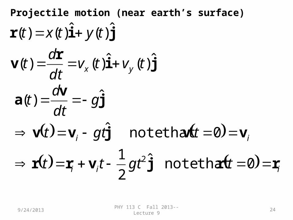
Projectile motion (near earth’s surface)
jir
v
jir
ˆ)(ˆ)()(
ˆ)(ˆ)()(
tvtvdt
dt
tytxt
yx
iii
ii
tgttt
tgtt
gdt
dt
rrjvrr
vvjvv
jv
a
0 that note ˆ2
1
0 that note ˆ
ˆ)(
2

PHY 113 C Fall 2013-- Lecture 9 259/24/2013
Projectile motion (near earth’s surface) Trajectory equation in vector form:
ˆ)( jvv gtt i jvrr ˆ221 gttt ii
Aside: The equations for position and velocity written in this way are call “parametric” equations. They are related to each other through the time parameter.
Trajectory equation in component form:
2
21 gttvyty
tvxtx
yii
xii
gtvtv
vtv
yiy
xix
)(
)(

PHY 113 C Fall 2013-- Lecture 9 269/24/2013
Diagram of various trajectories reaching the same height h=1 m:
y
xq

PHY 113 C Fall 2013-- Lecture 9 279/24/2013
Projectile motion (near earth’s surface)
Trajectory path y(x); eliminating t from the equations:
Trajectory equation in component form:
2
212
21 sin
cos
gttvygttvyty
tvxtvxtx
iiiyii
iiixii
gtvgtvtv
vvtv
iiyiy
iixix
sin)(
cos)(
2
21
2
21
costan
coscossin
cos
ii
iiii
ii
i
ii
iiii
ii
i
v
xxgxxyxy
v
xxg
v
xxvyxy
v
xxt

PHY 113 C Fall 2013-- Lecture 9 289/24/2013
Isaac Newton, English physicist and mathematician (1642—1727)
http://www.newton.ac.uk/newton.html
1. In the absence of a net force, an object remains at constant velocity or at rest.
2. In the presence of a net force F, the motion of an object of mass m is described by the form F=ma.
3. F12 =– F21.

PHY 113 C Fall 2013-- Lecture 9 299/24/2013
Newton’s second law
F = m a
Types of forces:
Fundamental Approximate Empirical
Gravitational F=-mg j Friction
Electrical Support
Magnetic Elastic
Elementary
particles
PHY 113 C Fall 2013-- Lecture 9 309/24/2013
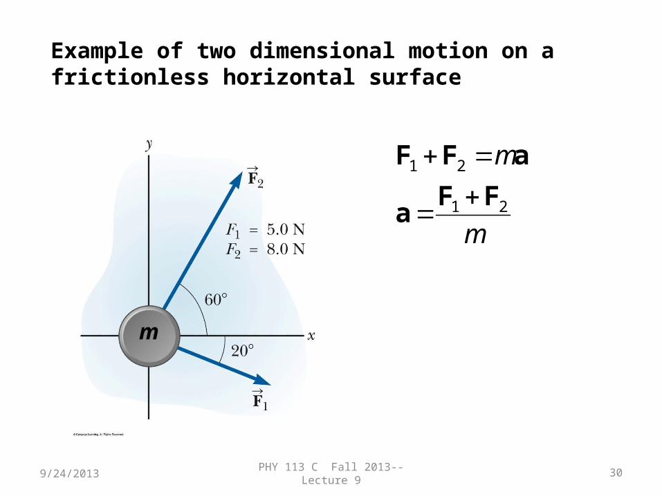
Example of two dimensional motion on a frictionless horizontal surface
m
m
m
21
21
FFa
aFF

PHY 113 C Fall 2013-- Lecture 9 319/24/2013
Example – support forces
appliedsupport
ˆ
FF
yF
mgg
Fsupport acts in direction to surface
(in direction of surface “normal”)

PHY 113 C Fall 2013-- Lecture 9 329/24/2013
Example of forces in equilibrium

PHY 113 C Fall 2013-- Lecture 9 339/24/2013
Example: 2-dimensional forcesA car of mass m is on an icy (frictionless) driveway, inclined at an angle t as shown. Determine its acceleration.
Conveniently tilted coordinate system:
sin
sin : Along
0cos : Along
ga
mamgx
mgny
x
x

PHY 113 C Fall 2013-- Lecture 9 349/24/2013
vi
vf=0
tgvtv
tgtvxtx
i
ii
sin)(
sin)( :incline Along 221
Another example: Note: we are using a tilted coordinate frame
i
mg
mg sin q

PHY 113 C Fall 2013-- Lecture 9 359/24/2013
Friction forces
The term “friction” is used to describe the category of forces that oppose motion. One example is surface friction which acts on two touching solid objects. Another example is air friction. There are several reasonable models to quantify these phenomena.
Surface friction:
N
Ff applied
Material-dependent coefficient
Normal force between surfaces
Air friction:
speedhigh at
speed lowat 2vK
KvD
K and K’ are materials and shape dependent constants

PHY 113 C Fall 2013-- Lecture 9 369/24/2013
Models of surface friction forces
(applied force)
surf
ace
fric
tion
forc
e
fs,max=msn
Coefficients ms , mk depend on the surfaces; usually, ms > mk

PHY 113 C Fall 2013-- Lecture 9 379/24/2013
mg
f
n
mg sin
mg cos
Consider a stationary block on an incline:
sincosThen
cos If
sin 0sin
cos 0cos
max,
mgmg
mgnff
mgfmgf
mgnmgn
S
SSS
tanS

PHY 113 C Fall 2013-- Lecture 9 389/24/2013
V (constant)
q
mg
n
f=mkn
Consider a block sliding down an inclined surface; constant velocity case
sincosThen
cos If
sin 0sin
cos 0cos
mgmg
mgnf
mgfmgf
mgnmgn
K
KK
tanK

PHY 113 C Fall 2013-- Lecture 9 399/24/2013
mg
f
n
mg sin
mg cos
Summary
slip about tojust isblock when tan
elocityconstant vat movesblock when tan
S
K

PHY 113 C Fall 2013-- Lecture 9 409/24/2013
Uniform circular motion and Newton’s second law
r
ra
aF
ˆ2
r
v
m
c

PHY 113 C Fall 2013-- Lecture 9 419/24/2013
rFr
rdW
f
i
fi
Definition of work: F
dr
ri rj
cal 0.239 J 1
JoulesmetersNewtons Work
: workof Units

PHY 113 C Fall 2013-- Lecture 9 429/24/2013
Example:
JmNmNdxFdWf
i
f
i
x
x
xfi 2525)4)(5( 21 rF
r
r

PHY 113 C Fall 2013-- Lecture 9 439/24/2013
Work and potential energy
rFr
r
dWf
i
fi : workof Definition
rFrr
r
r dWUref
ref
:energy potential of Definition
Note: It is assumed that F is conservative

PHY 113 C Fall 2013-- Lecture 9 449/24/2013
rFr
r
dWf
i
fi : workof Definition
Review of energy concepts:
2
2
1 :energy kinetic of Definition mvK
22
2
1
2
1
:oremenergy the kinetic-Work
if
f
i
totaltotalfi mvmvdW rF

PHY 113 C Fall 2013-- Lecture 9 459/24/2013
22
2
1
2
1
:oremenergy the kinetic-Work
if
f
i
totaltotalfi mvmvdW rF
Summary of work, potential energy, kinetic energy relationships
edissipativ
fiiiff
ifedissipativ
fiiftotalfi
WUKUK
KKWUUW
:gRearrangin
rr
edissipativfiif
edissipativfi
veconservatifi
totalfi
WUU
WWW

PHY 113 C Fall 2013-- Lecture 9 469/24/2013
Example problem from Webassign #8
A baseball outfielder throws a 0.150-kg baseball at a speed of 37.2 m/s and an initial angle of 31.0°. What is the kinetic energy of the baseball at the highest point of its trajectory?
vi
qi
yf
vf

PHY 113 C Fall 2013-- Lecture 9 479/24/2013
Example problem from Webassign #8
The coefficient of friction between the block of mass m1 = 3.00 kg and the surface in the figure below is μk = 0.440. The system starts from rest. What is the speed of the ball of mass m2 = 5.00 kg when it has fallen a distance h = 1.85 m?h
hf
ghmghmvmm
WUUKK
ghmfhW
WUKUK
kf
edissipativfifiif
kedissipativ
fi
edissipativfiiiff
122
21
1
02
1

PHY 113 C Fall 2013-- Lecture 9 489/24/2013
Example problem from Webassign #8
A block of mass m = 3.40 kg is released from rest from point A and slides on the frictionless track shown in the figure below. (Let ha =
6.70 m.) .

PHY 113 C Fall 2013-- Lecture 9 499/24/2013
Example problemfrom 2012 Exam #2:
if
if
veconservatifi
xUxU
UU
W

PHY 113 C Fall 2013-- Lecture 9 509/24/2013
Example problem from Webassign #5
013 gmT
0sinsin
0coscos
32211
2211
TTT
TT