9. a comparison of nonlinear, second order cone and linear
TRANSCRIPT

A comparison of nonlinear, second order cone and linear programming formulations for the optimal power flow problem
Jose Nicolas Melchor Gutierrez – UNESP ‐ UniMelb
Rubén A. Romero Lazaro – UNESP
Pierluigi Mancarella ‐ UniMelb

2
Optimal Power Flow

What is the Optimal Power Flow?
3
Optimal Power Flow
The OPF defines a set of electrical power systems problems that are subjected to power flow constraints and other operational constraints.
Economical dispatch
Optimal reactive power dispatch
Unit Commitment
.
.
.
OPF
What is the importance of the economical dispatch?
4
Optimal Power Flow
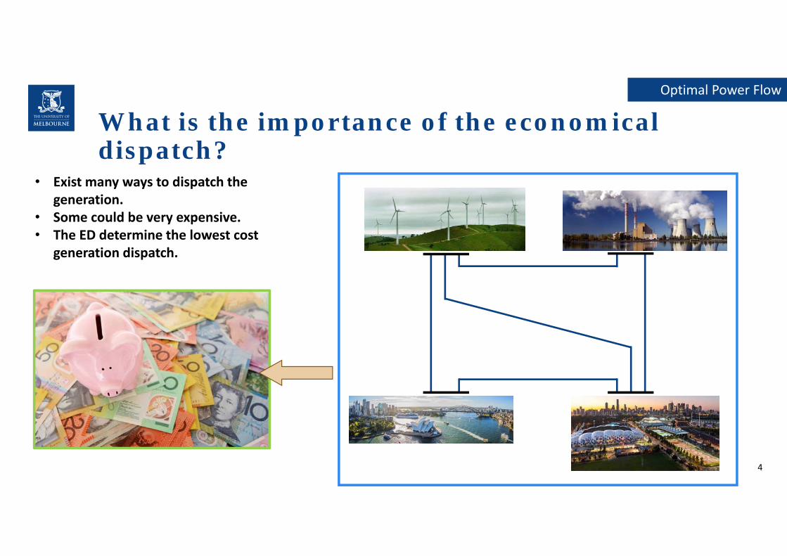
• Exist many ways to dispatch the generation.
• Some could be very expensive.• The ED determine the lowest cost
generation dispatch.

Why is it important to improve the OPF mathematical formulation?
5
Optimal Power Flow
[1] ‘Australian Energy Update’, Department of the Environment and Energy, Australia, 2017.[2] S. Letts, ‘Power prices are 'off the chart' and there's no relief in sight’, ABC News, July 7, 2017. [Online].
Available: http://www.abc.net.au/news/2017‐07‐07/power‐prices‐off‐the‐chart/8687480.[Accessed June 1, 2018].
= AUD$ 26728 Millions
AUD$ 1300 Millions
5%
257.000.000 MWh
[1] 104 AUD$/MWh
[2]
X

6
OPF formulations

Non ConvexMultimodal
Polar Power and Voltage - Nonlinear
7
OPF formulations
Objective function.
2 2 1 0min ( )( )g
g g g g gn n n n n
nC p C p C
2( , , )( , , )
( , , ) ( , , )l l
fromg to sh dn l n m n n nl n m
l n m l n mn m n m
p P P g v P
2( , , )( , , )
( , , ) ( , , )l l
fromg to sh dn l n m n n nl n m
l n m l n mn m n m
q Q Q b v Q
Power balance.
2 2( , , ) ( , , ) ( , , ) ( , , ) ( , , ) ( , , ) ( , , )( , , ) cos( ) sin( )( ) froml n m n l n m l n m n m l n m n m l n m l n m n m l n ml n mP a v g a v v g b
2 2( , , ) ( , , ) ( , , ) ( , , ) ( , , ) ( , , ) ( , , ) ( , , )( , , ) sin( ) cos( ) ( )( ) from shl n m n m l n m n m l n m l n m n m l n m l n m n l n m l n ml n mQ a v v g b a v b b
2( , , ) ( , , ) ( , , ) ( , , ) ( , , ) ( , , ) ( , , )cos( ) sin( )( ) tol n m m l n m l n m n m l n m n m l n m l n m n m l n mP v g a v v g b
2( , , ) ( , , ) ( , , ) ( , , ) ( , , ) ( , , ) ( , , ) ( , , )sin( ) cos( ) ( )( ) to shl n m l n m n m l n m n m l n m l n m n m l n m m l n m l n mQ a v v g b v b b
Power flow equations.
min maxn n nv v v 2 2 2
( , , )( , , ) ( , , )( ) ( ) ( )from from maxl n ml n m l n mP Q S
2 2 2( , , ) ( , , ) ( , , )( ) ( ) ( )to to maxl n m l n m l n mP Q S min g max
n n nP p Pmin g maxn n nQ q Q
Bounds.
Trigonometric functions.Product of variables.Equality constraints.
Convex quadratic constraints.
Squared variables.Equality constraints.
Convex constraints.

Polar Power and Voltage – Second Order Cone
8
OPF formulations
2
2n
nuv
( , , ( , , )) sin( ) n m n m ll m nn mv v
( , , ( , , )) cos( ) n m n m ll m nn mv v
2 2( , , ) ( , , )2 n m l n m l n mu u
Substitutions
Original Constraints
Power balance.
( , , )( , , )( , , ) ( , , )
2
l l
fromg to sh dn l n m n nl n m
l n m l mn
nn
m n m
p uP P g P
( , , )( , , )( , , ) ( , , )
2
l l
fromg to sh dn l n m n nl n m
l n m l mn
nn
m n m
q uQ Q b Q
Power flow equations.
2( , , ) ( ( ,, , ) ( , , ) ( , , ) ( , , ), ) ( , ,( , ), ) 2 ( ) froml n m l n m l n m l n m l nn l n ml m lm nn mP a g au g b
2( , , ) ( , , ) ( , ,( , , ) ( ,) ( , , ) ( , , ) ( , , )( , , ) , ) 2 ( )( ) l n m l n m
from shl n m l n m l n m l n m l n m l n ml n m nQ a g b a b bu
( , , ) ( , , ) ( , , ) ( , , ) ( ,( , , ) , ) ( , , ))2 ( ) m l n m l ntol n m l n m l n m l n m l mn mP g a g bu
( , , ) ( , , ) ( , , ) ( , , ) ( , , ) (( , , ) ( )) ,, ,, ( )2( ) to shl n m l n m l n m ll n m ln m n l n m lm nm mQ b b bua g
2 2 2( , , )( , , ) ( , , )( ) ( ) ( )from from maxl n ml n m l n mP Q S
2 2 2( , , ) ( , , ) ( , , )( ) ( ) ( )to to maxl n m l n m l n mP Q S min g max
n n nP p Pmin g maxn n nQ q Q
Bounds. 2 2
2 2
min maxn n
n
v vu
AdditionalConstraints
2 2( , , ) ( , , )2 n m l n m l n mu u
( ,( , , ) , ) l n m n m l n m
1nv
( , , ) ( , , )sin( ) n m l n m n m l n m
Approximations

Polar Power and Voltage – Second Order Cone
9
OPF formulations
Power balance.
( , , )( , , )( , , ) ( , , )
2
l l
fromg to sh dn l n m n nl n m
l n m l mn
nn
m n m
p uP P g P
( , , )( , , )( , , ) ( , , )
2
l l
fromg to sh dn l n m n nl n m
l n m l mn
nn
m n m
q uQ Q b Q
Power flow equations.
2( , , ) ( ( ,, , ) ( , , ) ( , , ) ( , , ), ) ( , ,( , ), ) 2 ( ) froml n m l n m l n m l n m l nn l n ml m lm nn mP a g au g b
2( , , ) ( , , ) ( , ,( , , ) ( ,) ( , , ) ( , , ) ( , , )( , , ) , ) 2 ( )( ) l n m l n m
from shl n m l n m l n m l n m l n m l n ml n m nQ a g b a b bu
( , , ) ( , , ) ( , , ) ( , , ) ( ,( , , ) , ) ( , , ))2 ( ) m l n m l ntol n m l n m l n m l n m l mn mP g a g bu
( , , ) ( , , ) ( , , ) ( , , ) ( , , ) (( , , ) ( )) ,, ,, ( )2( ) to shl n m l n m l n m ll n m ln m n l n m lm nm mQ b b bua g
2 2 2( , , )( , , ) ( , , )( ) ( ) ( )from from maxl n ml n m l n mP Q S
2 2 2( , , ) ( , , ) ( , , )( ) ( ) ( )to to maxl n m l n m l n mP Q S min g max
n n nP p Pmin g maxn n nQ q Q
Bounds. 2 2
2 2
min maxn n
n
v vu
AdditionalConstraints
2 2( , , ) ( , , )2 n m l n m l n mu u
( ,( , , ) , ) l n m n m l n m
Linear Constraints.
Linear Constraints.Conic Constraints.
ConvexGlobal Optima

DC Power Flow- Linear
10
OPF formulations
Objective function.
2 2 1 0min ( )( )L
g
g g g g gn n n n n
nC p C p C Piecewise linear function
Power balance.
( , , ) ( , , )( , , ) ( , , )
l l
g dn l n m l m n n
l n m l m np P P P
Power flow equations. ( , , ) ( , , ) ( , , ) l n m l n m n m l n mP b
min g maxn n nP p PBounds.( , , ) ( , , ) ( , , ) max maxl n m l n m l n mP P P
1nv
( , , ) ( , , )sin( ) n m l n m n m l n m
Approximations
( , , ) ( , , )l n m l n mr x
( , , )l n mQX
( , , )cos( ) 1 n m l n m

11
Simulations and Results
Test system and optimisation tools
12
Simulations and Results
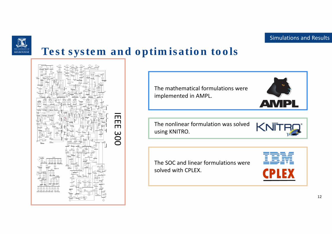
The mathematical formulations were implemented in AMPL.
The nonlinear formulation was solved using KNITRO.
The SOC and linear formulations were solved with CPLEX.
IEEE 300

Active Power Generation and Cost
13
Simulations and Results
0
400
800
1200
1600
2000
MW
Generation
Nonlinear Conic Linear
Cost US$/hrNonlinear 722670,42Conic 721707,75Linear 709066,95
Generation (MW)Nonlinear 23690,15Conic 23681,31Linear 23391,01

Active Power Generation and Cost
14
Simulations and Results
Cost US$/hrNonlinear 722670,42Conic 721707,75Linear 709066,95
Generation (MW)Nonlinear 23690,15Conic 23681,31Linear 23391,01
Full AC PF
Generation Dispatch
Solution Load SheddingLosses
DC or SOC
Testing the feasibility of the
solutions

Active Power Generation and Cost
15
Simulations and Results
0
400
800
1200
1600
2000
MW
Generation
Nonlinear Conic Linear
Load Shedding (MW)SOC 37,32Linear 1005,76
Infeasible!

Voltage Angle Difference
16
Simulations and Results
‐5
0
5
10
15
20
230 144 80 143 129 327 140 195 78 369
Degree
s
Bus number
Maximum Angular Difference
Nonlinear Conic Linear
‐20
‐15
‐10
‐5
0
5
10
15
20
1(3) 2(7) 3(29) 4(28) 5(82) 6(5) 7(19) 8(91) 9(61) 10(48)
Degree
s
Cluster
K‐means Clustered Angular Difference
Nonlinear Conic Linear

Voltage Angle Difference
17
Simulations and Results
‐5
0
5
10
15
20
230 144 80 143 129 327 140 195 78 369
Degree
s
Bus number
Maximum Angular Difference
Nonlinear Conic Linear

Conic Constraints Approximation Error
18
Simulations and Results
0.00
0.02
0.04
0.06
0.08
0.10
0.12
0.14
0.16
0.18
0.20
1 31 61 91 121 151 181 211 241 271 301 331 361
Absolute error
Circuit number
Conic Constraints error

19
Conclusions
Preliminary Conclusions
20
Conclusions
In this preliminary research the solution obtained with the DC OPF and the second order coneapproximations are infeasible for the full AC OPF representing the IEEE‐300 test system withpower limit for the transmission lines and transformers. However, further studies need to bedone in order to determine if these results are particular for this test system or if a fundamentalproblem has been detected.
