8:38:34 pmics 573: high-performance computing11.1 search algorithms for discrete optimization...
Post on 22-Dec-2015
231 views
TRANSCRIPT
8:38:34 PM ICS 573: High-Performance Computing 11.1
Search Algorithms for Discrete Optimization Problems
• Discrete Optimization - Basics
• Sequential Search Algorithms
• Parallel Depth-First Search
• Parallel Best-First Search
• Speedup Anomalies in Parallel Search Algorithms
8:38:34 PM ICS 573: High-Performance Computing 11.2
Discrete Optimization Problems
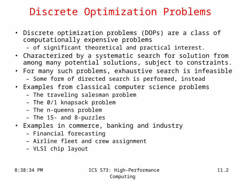
• Discrete optimization problems (DOPs) are a class of computationally expensive problems – of significant theoretical and practical interest.
• Characterized by a systematic search for solution from among many potential solutions, subject to constraints.
• For many such problems, exhaustive search is infeasible– Some form of directed search is performed, instead
• Examples from classical computer science problems– The traveling salesman problem– The 0/1 knapsack problem– The n-queens problem– The 15- and 8-puzzles
• Examples in commerce, banking and industry– Financial forecasting– Airline fleet and crew assignment– VLSI chip layout
8:38:34 PM ICS 573: High-Performance Computing 11.3
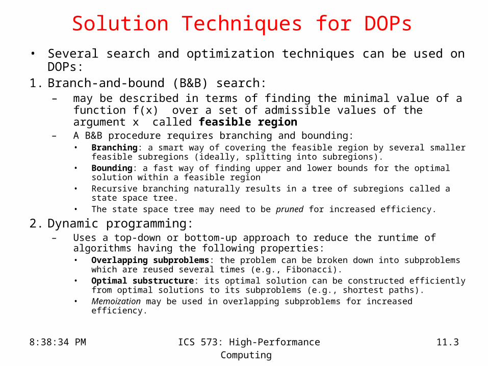
Solution Techniques for DOPs • Several search and optimization techniques can be used on DOPs:1. Branch-and-bound (B&B) search:
– may be described in terms of finding the minimal value of a function f(x) over a set of admissible values of the argument x called feasible region
– A B&B procedure requires branching and bounding:• Branching: a smart way of covering the feasible region by several smaller feasible
subregions (ideally, splitting into subregions).• Bounding: a fast way of finding upper and lower bounds for the optimal solution within
a feasible region• Recursive branching naturally results in a tree of subregions called a state space tree.• The state space tree may need to be pruned for increased efficiency.
2. Dynamic programming: – Uses a top-down or bottom-up approach to reduce the runtime of algorithms
having the following properties:• Overlapping subproblems: the problem can be broken down into subproblems which
are reused several times (e.g., Fibonacci).• Optimal substructure: its optimal solution can be constructed efficiently from optimal
solutions to its subproblems (e.g., shortest paths). • Memoization may be used in overlapping subproblems for increased efficiency.
8:38:34 PM ICS 573: High-Performance Computing 11.4
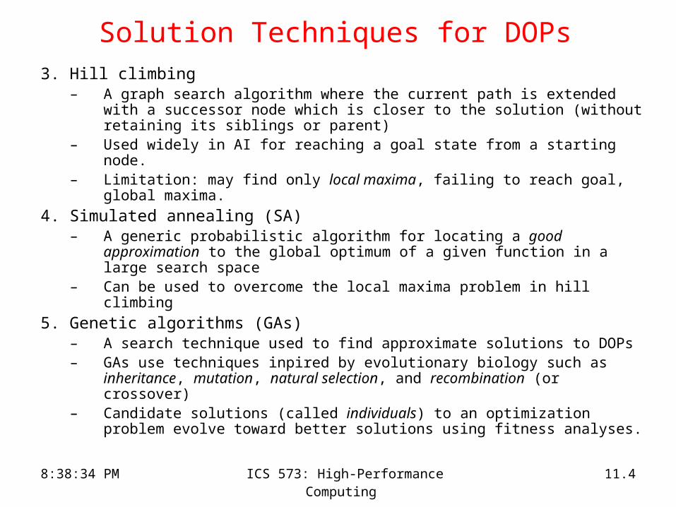
Solution Techniques for DOPs 3. Hill climbing
– A graph search algorithm where the current path is extended with a successor node which is closer to the solution (without retaining its siblings or parent)
– Used widely in AI for reaching a goal state from a starting node.– Limitation: may find only local maxima, failing to reach goal, global
maxima.
4. Simulated annealing (SA)– A generic probabilistic algorithm for locating a good approximation to
the global optimum of a given function in a large search space– Can be used to overcome the local maxima problem in hill climbing
5. Genetic algorithms (GAs)– A search technique used to find approximate solutions to DOPs– GAs use techniques inpired by evolutionary biology such as
inheritance, mutation, natural selection, and recombination (or crossover)
– Candidate solutions (called individuals) to an optimization problem evolve toward better solutions using fitness analyses.
8:38:34 PM ICS 573: High-Performance Computing 11.5
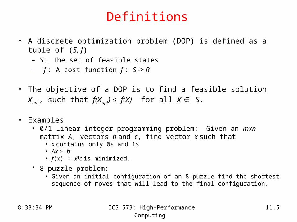
Definitions
• A discrete optimization problem (DOP) is defined as a tuple of (S, f)– S : The set of feasible states– f : A cost function f : S -> R
• The objective of a DOP is to find a feasible solution xopt, such that
f(xopt) ≤ f(x) for all x S.
• Examples• 0/1 Linear integer programming problem: Given an mxn matrix A,
vectors b and c, find vector x such that• x contains only 0s and 1s• Ax > b• f(x) = xTc is minimized.
• 8-puzzle problem: • Given an initial configuration of an 8-puzzle find the shortest sequence of
moves that will lead to the final configuration.
8:38:34 PM ICS 573: High-Performance Computing 11.6
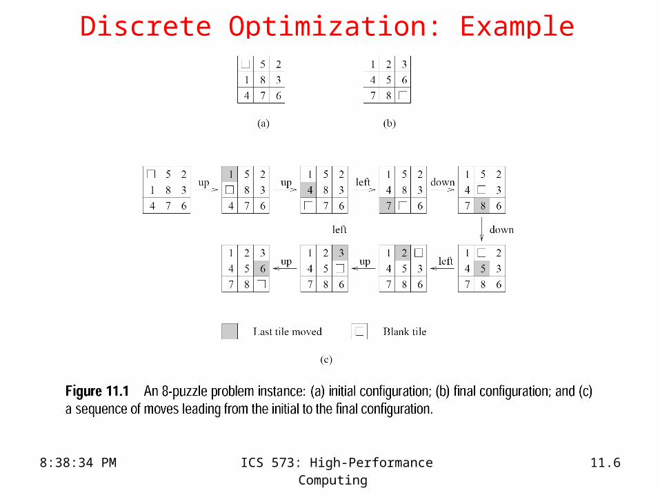
Discrete Optimization: Example
8:38:34 PM ICS 573: High-Performance Computing 11.7
Formulating DOPs as Graph Search
• The feasible space S is typically very large.
• Many DOP can be formulated as finding the minimum cost path in a graph.– Nodes in the graph correspond to states.– States are classified as either
• terminal or non-terminal
– Some of the states correspond to feasible solutions whereas others do not.
– Edges correspond to “costs” associated with moving from one state to the other.
• These graphs are called state-space graphs.
8:38:34 PM ICS 573: High-Performance Computing 11.8
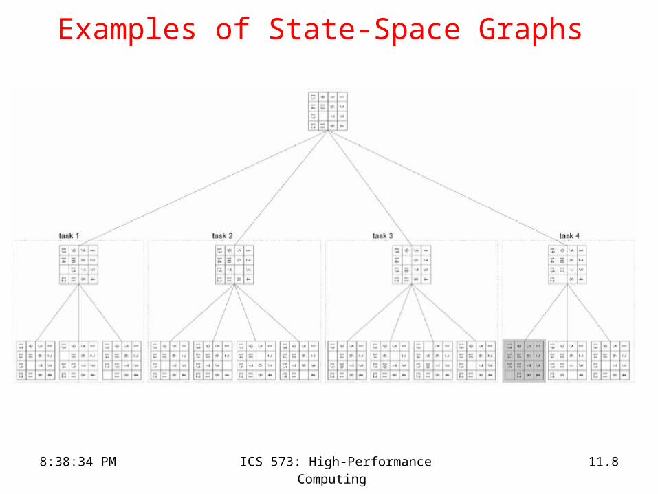
Examples of State-Space Graphs
8:38:34 PM ICS 573: High-Performance Computing 11.9
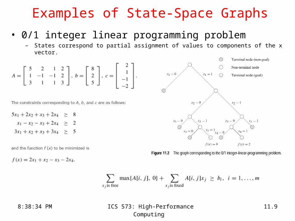
Examples of State-Space Graphs
• 0/1 integer linear programming problem– States correspond to partial assignment of values to components of the x vector.
8:38:34 PM ICS 573: High-Performance Computing 11.10
Admissible Heuristics • Often, it is possible to estimate the cost to reach the goal state from an
intermediate state.
• This estimate, called a heuristic estimate, can be effective in guiding search to the solution.
• If the estimate is guaranteed to be an underestimate, the heuristic is called an admissible heuristic.
• Admissible heuristics have desirable properties in terms of optimality of solution (as we shall see later).
• An admissible heuristic for 8-puzzle is as follows: – Assume that each position in the 8-puzzle grid is represented as a pair. – The distance between positions (i,j) and (k,l) is defined as |i -
k| + |j - l|. This distance is called the Manhattan distance. – The sum of the Manhattan distances between the initial and final positions of
all tiles is an admissible heuristic.
8:38:34 PM ICS 573: High-Performance Computing 11.11
Parallel Discrete Optimization: Motivation
• DOPs are generally NP-hard problems. Does parallelism really help much?– Cannot reduce their worst-case running time to a polynomial one
• For many problems, the average-case runtime is polynomial.
• Often, we can find suboptimal solutions in polynomial time.– Bigger problem instances can be solved
• Many DOPs have smaller state spaces but require real-time
solutions. – Parallel processing may be the only way to obtain acceptable
performance!
8:38:34 PM ICS 573: High-Performance Computing 11.12
Exploring the State-Space Graphs
• The solution is discovered by exploring the state-space search.– Exponentially large
• Heuristic estimates of the solution cost are used.– Cost of reaching to a feasible solution from current state x is
l(x) = g(x) + h(x)
• Admissible heuristics are the heuristics that correspond to lower bounds on the actual cost.– Manhattan distance is an admissible heuristic for the 8-puzzle problem.
• Idea is to explore the state-space graph using heuristic cost estimates to guide the search.– Do not spend any time exploring “bad” or “unpromising” states.
8:38:34 PM ICS 573: High-Performance Computing 11.13
Search Space Structure: Trees Vs Graphs
• Is the search space a tree or a graph?
• Trees– Each new successor leads to an unexplored part of the search space.– Example: the space of a 0/1 integer linear programming
• Graphs– A state can be reached along multiple paths. – Whenever a state is generated, it is necessary to check if the state has
already been generated.– Example: the space of 8-puzzle.
• Next, we consider sequential solution strategies for DOPs formulated as tree or graph search problems.
8:38:34 PM ICS 573: High-Performance Computing 11.14
Sequential Exploration Strategies
1. Depth-Firsti. Simple Backtracking
– Performs DFS until it finds the first feasible solution and terminates– Uses no heuristic to order the successors of the expanded node– Not guaranteed to find optimal solution– Ordered backtracking uses heuristics to order successors
ii. Depth-First Branch-and-Bound (DFBB)– Partial solutions that are inferior to the current best solutions are discarded.– Does not explore paths leading to inferior solutions
iii. Iterative Deepening– Tree is expanded up to certain depth.– If no feasible solution is found, the depth is increased and the entire process
is repeated.– Useful when solution exists close to root on alternative branch
iv. Iterative Deepening A* (IDA*)– Imposes cost-bound rather than a depth-bound– Finds an optimal solution when an admissible heuristic is used
8:38:34 PM ICS 573: High-Performance Computing 11.15
DFS Storage Requirements and Data Structures
• Suitable primarily for state-graphs that are trees
• At each step of DFS, untried alternatives must be stored for backtracking.
• If m is the amount of storage required to store a state, and d is the maximum depth, then the total space requirement of the DFS algorithm is O(md).
• The state-space tree searched by parallel DFS can be efficiently represented as a stack.
• Memory requirement of the stack is linear in depth of tree.
8:38:34 PM ICS 573: High-Performance Computing 11.16
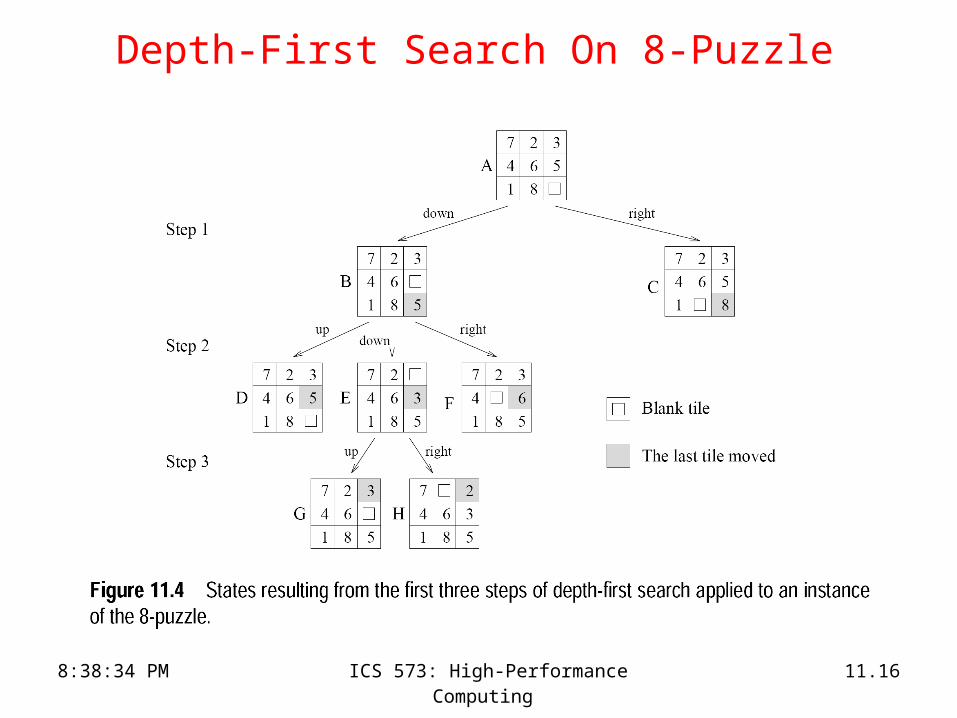
Depth-First Search On 8-Puzzle

8:38:34 PM ICS 573: High-Performance Computing 11.17
Representing a DFS Tree
8:38:34 PM ICS 573: High-Performance Computing 11.18
Sequential Exploration Strategies
2. Best-First Search (BFS)– BFS algorithms use a heuristic to guide search.
– If the heuristic is admissible, the BFS finds the optimal solution. – OPEN/CLOSED lists
– A* algorithm• Heuristic estimate is used to order the nodes in the open list.
• Suitable for state-space graphs that are either trees or graphs.
• Large memory complexity.– Proportional to the number of states visited.
8:38:34 PM ICS 573: High-Performance Computing 11.19
Data Structures for BFS Algorithms
• The core data structure is a list, called open list, that stores unexplored nodes sorted on their heuristic estimates.
• The best node is selected from the list, expanded, and its off-spring are inserted at the right position.
• BFS of graphs must be slightly modified to account for multiple paths to the same node.
• A closed list stores all the nodes that have been previously seen.
• If a newly expanded node exists in the open or closed lists with better heuristic value, the node is not inserted into the open list.
8:38:34 PM ICS 573: High-Performance Computing 11.20
The A* Algorithm
• A BFS technique that uses admissible heuristics.
• Defines function l(x) for each node x as g(x) + h(x).
• Here, g(x) is the cost of getting to node x and h(x) is an admissible heuristic estimate of getting from node x to the solution.
• The open list is sorted on l(x).
• The space requirement of BFS is exponential in depth!
8:38:34 PM ICS 573: High-Performance Computing 11.21
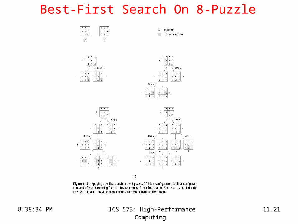
Best-First Search On 8-Puzzle
8:38:34 PM ICS 573: High-Performance Computing 11.22
Search Overhead Factor
• The amount of work done by serial and parallel formulations of search algorithms is often different.
– Why?
• Let W be serial work and WP be parallel work.
– Search overhead factor s is defined as WP/W.
• Upper bound on speedup is p×(W/WP).
• Assumptions for subsequent analyses:– the time to expand each node, tc, is the same– W and Wp are the number of nodes expanded by the serial and the parallel formulations,
respectively. – From the above, the sequential run time is given by TS = tcW.
– We assume that tc = 1.
8:38:34 PM ICS 573: High-Performance Computing 11.23
Parallel Depth-First Search Challenges
• Computation is dynamic and unstructured– Why dynamic?– Why unstructured?
• Decomposition approaches?– Do we do the same work as the sequential algorithm?
• Mapping approaches?– How do we ensure load balance?– Static partitioning of unstructured trees yields poor performance.
• Dynamic load balancing is required.
8:38:34 PM ICS 573: High-Performance Computing 11.24
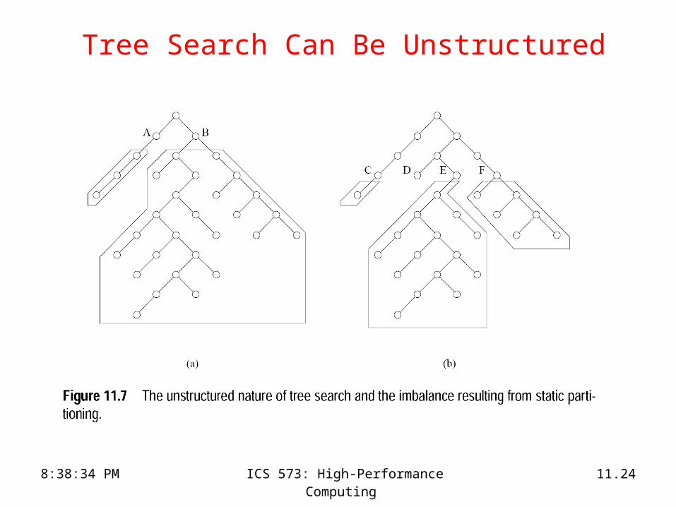
Tree Search Can Be Unstructured
8:38:34 PM ICS 573: High-Performance Computing 11.25
Parallel DFS: Dynamic Load Balancing
• When a processor runs out of work, it gets more work from another processor. – Trades communication cost for load balancing
• This is done using – work requests and responses in message passing machines, and
– locking and extracting work in shared address space machines.
• On reaching final state at a processor, all processors terminate.
• Unexplored states can be conveniently stored as local stacks at processors.
• The entire space is assigned to one processor to begin with.
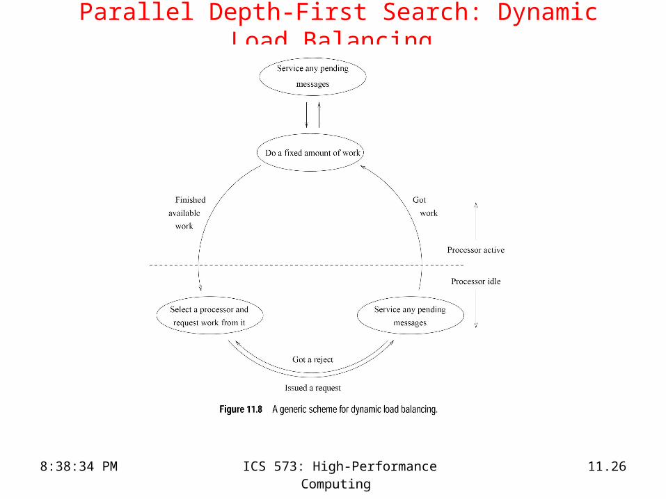
8:38:34 PM ICS 573: High-Performance Computing 11.26
Parallel Depth-First Search: Dynamic Load Balancing
8:38:34 PM ICS 573: High-Performance Computing 11.27
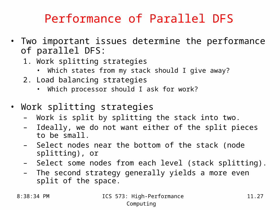
Performance of Parallel DFS
• Two important issues determine the performance of parallel DFS:1. Work splitting strategies
• Which states from my stack should I give away?
2. Load balancing strategies• Which processor should I ask for work?
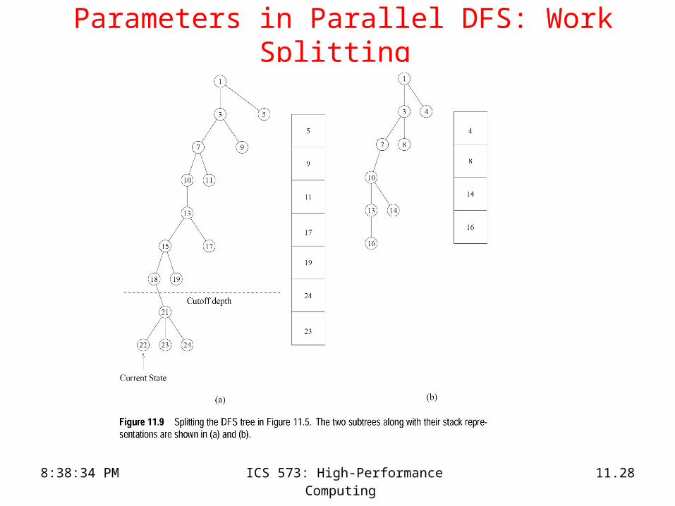
• Work splitting strategies – Work is split by splitting the stack into two.– Ideally, we do not want either of the split pieces to be small.– Select nodes near the bottom of the stack (node splitting), or– Select some nodes from each level (stack splitting). – The second strategy generally yields a more even split of the
space.
8:38:34 PM ICS 573: High-Performance Computing 11.28
Parameters in Parallel DFS: Work Splitting
8:38:34 PM ICS 573: High-Performance Computing 11.29
Load-Balancing Schemes
• Who do you request work from? – Note: we would like to distribute work requests evenly, in a global
sense.
• Asynchronous round robin: – Each processor maintains a counter and makes requests in a round-
robin fashion.– Work requests are generated independently by each processor.
• Global round robin: – The system maintains a global counter and requests are made in a
round-robin fashion, globally.– Ensures that successive work requests are distributed evenly over all
processors.
• Random polling: – Request a randomly selected processor for work.
8:38:34 PM ICS 573: High-Performance Computing 11.30
Termination Detection
• How do you know when everyone's done?
• A number of algorithms have been proposed.
8:38:34 PM ICS 573: High-Performance Computing 11.31
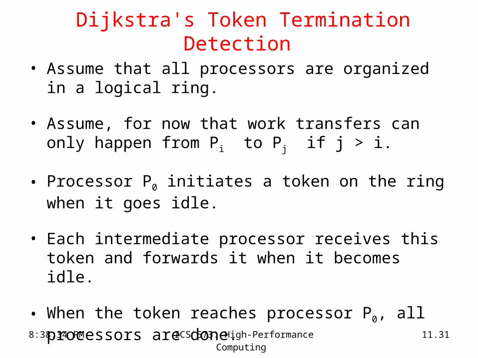
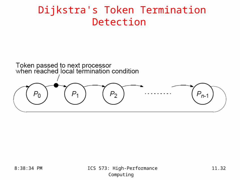
Dijkstra's Token Termination Detection
• Assume that all processors are organized in a logical ring.
• Assume, for now that work transfers can only happen from Pi to Pj if j > i.
• Processor P0 initiates a token on the ring when it goes idle.
• Each intermediate processor receives this token and forwards it when it becomes idle.
• When the token reaches processor P0, all processors are done.
8:38:34 PM ICS 573: High-Performance Computing 11.32
Dijkstra's Token Termination Detection

8:38:34 PM ICS 573: High-Performance Computing 11.33
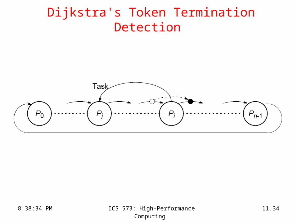
Dijkstra's Token Termination Detection • When processor P0 goes idle, it colors itself green and initiates
a green token.
• If processor Pj sends work to processor Pi and j > i then processor Pj becomes red.
• If processor Pi has the token and Pi is idle, it passes the token to Pi+1. – If Pi is red, then the color of the token is set to red before it is sent to
Pi+1.
– If Pi is green, the token is passed unchanged.
• After Pi passes the token to Pi+1, Pi becomes green .
• The algorithm terminates when processor P0 receives a green token and is itself idle.
8:38:34 PM ICS 573: High-Performance Computing 11.34
Dijkstra's Token Termination Detection
8:38:34 PM ICS 573: High-Performance Computing 11.35
Tree-Based Termination Detection
• Associate weights with individual workpieces. Initially, processor P0 has all the work and a weight of one.
• Whenever work is partitioned, the weight is split into half and sent with the work.
• When a processor gets done with its work, it sends its parent the weight back.
• Termination is signaled when the weight at processor P0 becomes 1 again.
• Note that underflow and finite precision are important factors associated with this scheme.
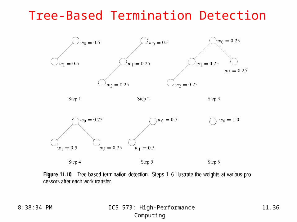
8:38:34 PM ICS 573: High-Performance Computing 11.36
Tree-Based Termination Detection
8:38:34 PM ICS 573: High-Performance Computing 11.37
Parallel Formulations of Depth-First Branch-and-Bound
• Parallel formulations of depth-first branch-and-bound search (DFBB) are similar to those of DFS.
• Each processor has a copy of the current best solution. This is used as a local bound.
• If a processor detects another solution, it compares the cost with current best solution. – If the cost is better, it broadcasts this cost to all processors.
• If a processor's current best solution path is worse than the globally best solution path, only the efficiency of the search is affected, not its correctness.
8:38:34 PM ICS 573: High-Performance Computing 11.38
Parallel Formulations of IDA*
• Common Cost Bound: – Each processor is given the same cost bound.
– Processors use parallel DFS on the tree within the cost bound.
– The drawback of this scheme is that there might not be enough
concurrency.
• Variable Cost Bound: – Each processor works on a different cost bound.– The major drawback here is that a solution is not guaranteed to
be optimal until all lower cost bounds have been exhausted.
• In each case, parallel DFS is the search kernel.
8:38:34 PM ICS 573: High-Performance Computing 11.39
Parallel Best-First Search
• The core data structure is the open list (typically implemented as a priority queue).
• Each processor locks this queue, extracts the best node, unlocks it.
• Successors of the node are generated, their heuristic functions estimated, and the nodes inserted into the open list as necessary after appropriate locking.
• Since we expand more than one node at a time, we may expand nodes that would not be expanded by a sequential algorithm.

8:38:34 PM ICS 573: High-Performance Computing 11.40
Parallel BFS: Centralized Lists
8:38:34 PM ICS 573: High-Performance Computing 11.41
Problems with Centralized Lists
• The termination criterion of sequential BFS fails for parallel BFS.– p nodes from the open list are being expanded
• The open list is a point of contention.– Can severely limit speedup even on shared-address-space
architectures
• Distributed open lists may address can help

8:38:34 PM ICS 573: High-Performance Computing 11.42
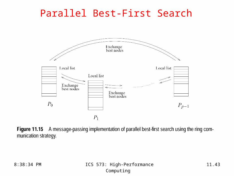
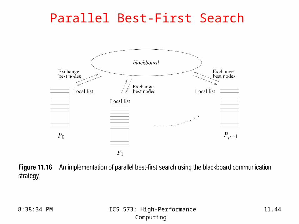
Parallel Best-First Search
• Avoid contention by having multiple open lists.
• Initially, the search space is statically divided across these open lists.
• Processors concurrently operate on these open lists.
• Since the heuristic values of nodes in these lists may diverge significantly,
– we must periodically balance the quality of nodes in each list.
• A number of balancing strategies based on ring, blackboard, or random communications are possible.
8:38:34 PM ICS 573: High-Performance Computing 11.43
Parallel Best-First Search
8:38:34 PM ICS 573: High-Performance Computing 11.44
Parallel Best-First Search
8:38:34 PM ICS 573: High-Performance Computing 11.45
Parallel Best-First Graph Search
• Graph search involves a closed list, where the major operation is a lookup (on a key corresponding to the state).
• The classic data structure is a hash.
• Hashing can be parallelized by using two functions:– the first one hashes each node to a processor, and – the second one hashes within the processor.
• This strategy can be combined with the idea of multiple open lists.
• If a node does not exist in a closed list, it is inserted into the open list at the target of the first hash function.
• In addition to facilitating lookup, randomization also equalizes quality of nodes in various open lists.

8:38:34 PM ICS 573: High-Performance Computing 11.46
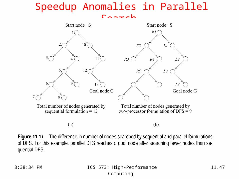
Speedup Anomalies in Parallel Search
• Since the search space explored by processors is determined dynamically at runtime, the actual work might vary significantly.
• Speedup anomalies using p processors:– acceleration anomalies: executions yielding speedups greater than p
– deceleration anomalies: executions yielding speedups of less than p
• Speedup anomalies also manifest themselves in best-first search algorithms.
• If the heuristic function is good, the work done in parallel best-first search is typically more than that in its serial counterpart.
8:38:34 PM ICS 573: High-Performance Computing 11.47
Speedup Anomalies in Parallel Search

8:38:34 PM ICS 573: High-Performance Computing 11.48
Speedup Anomalies in Parallel Search