8 international conference on the stability of ships...

8th International Conference on the Stability of Ships and Ocean Vehicles Escuela Técnica Superior de Ingenieros Navales

129

STUDY OF THE DYNAMIC STABILITY OF AN UNDERWATER VEHICLE

J. Fernández Ibarz, A. Lamas & F. López Peña Universidade da Coruña, Escuela Politécnica Superior. (Spain)

The problem of dynamic stability of motion of underwater vehicles is addressed by developing an analytical model of the underwater vehicle dynamics and by applying it using a simulator. The model’s equations of motion were obtained by combining theoretical formulae with experimental data, taking into account the coupling between the different forces and moments produced on the submersible by the surrounding fluid. All the terms included in the equations have been derived from scratch. A simplified procedure for obtaining the force, moment, and the added mass coefficients needed as input of the equations by using potential flow theory and adding viscous effects in the stern region is shown. Satisfactory results are obtained when applying the derived method to calculate these coefficients for submarines and airships documented in the literature. The derived equations of motion have been implemented in a simulator together with a model for the fins, rudders, and control surfaces. This simulator was used to perform a dynamic stability analysis of the motion of a submersible catamaran designed for tourist tours. Three different configurations of rudders were used; the analyses of the dynamic responses of the vehicle for different cases show that the vehicle is intrinsically unstable but easily controllable, as has been proven by using a controller developed specifically for this purpose. The use of genetic algorithms for developing this controller results in a very efficient tailored system. 1. INTRODUCTION No too long ago submarine vehicle design was almost exclusively restricted to military applications. Recently a variety of different applications has emerged, these are mainly autonomous underwater vehicles aimed for different purposes as well as some manned underwater vehicles devoted to research, exploration, survey or tourism. Particularly, the present work has been carried out within the framework of a project for a tourism submarine vehicle. Our goal is to obtain a dynamical model for a generic underwater vehicle, to apply it to this particular submarine and then to use it to study its stability and to develop its control system.

Publications describing the dynamics of underwater vehicles are quite sparse. Probably this is due to the fact that most of the related work is classified and therefore unpublished. Examples of publications containing general models of underwater vehicles are those by Brutzman [1] and Abkowitz [2]. Some other authors, such as Coxon [3], use the standard equations of motion for submarines by Feldman [4] and by Gertler and Hagen [5], both from the David W. Taylor Naval Ship Research and Development Center. In our case the dynamical model has been developed from scratch independently of the ones used in other studies of submarines. Nevertheless, after realising that the similarity parameters –Reynolds number and buoyancy to weight

8th International Conference on the Stability of Ships and Ocean Vehicles

Escuela Técnica Superior de Ingenieros Navales 130

ratio- of submarines and airships get their values in the same range, we have made use of the theoretical and experimental developments performed on the latter during the first third of the twentieth century. The vehicle object of the present study is a submersible catamaran and, consequently, it has a complex geometry. Figure 1 displays a sketch of the submarine and its main dimensions. The vessel has some thrusters to perform manoeuvres at a fixed point or near obstacles, these thrusters are not going to be considered in the present work as we attempt to focus on the manoeuvres governed by fins or rudders. In this paper we also present some simplified analytical tools allowing the estimation of forces, moments, and added mass coefficients altogether with a model to take into account the effects of fins and other governing surfaces. Stability analyses are performed on three models corresponding to three different configurations of these surfaces. 2. EQUATIONS OF MOTION The laws of conservation of momentum and angular momentum expressed in a system of cartesian coordinate axes fixed to the vehicle are:

VùVF ⊗+= &m

(1)

( )ùIùùIM ⋅⊗+⋅= & (2)

The force F and angular momentum M vectors account for the forces directly applied to the vehicle and their moments; that is for weight, buoyancy, drag, lift and thrust and their moments with respect to the vehicle’s centre of gravity. The inertia matrix I is a function of both the vehicle’s geometry and its weight distribution, but –as it happens in any submarine- the vehicle has a symmetry plane. Taking this plane as xz -represented in figure 1- then Ixy=Iyx=Iyz=Izy=0, and Ixz=Izx. The angular velocity ωω can be accounted for by the rotation needed to transform from body-fixed Fb to local horizon Fh coordinate systems, as shown in figure 2. The local horizon cartesian coordinate system has its origin in the centre of gravity of the vehicle, having its axes directions parallel to the ones given by a reference coordinate system fixed to the earth’s surface. According to this, and following the terminology in figure 2, the angle ψ represents the vehicle’s course, while φ is the vehicle’s balancing angle and θ is its climbing angle.

Figure 1 Sketch and main dimensions of the submarine


131

Calling ωω = (p, q, r) it is easy to obtain from figure 2:

φθψ && +−= sinp φθφθψ cossincos && +=q (3) φθφθψ sincoscos && −=r

Figure 2 Transformation from body-fixed to local horizon coordinate axes. Consider now the forces and moments exerted on the vehicle. On one hand we have thrust, weight, and buoyancy and their moments with respect to the center of gravity, all of these should be known for the vehicle’s current configuration. In addition we should consider some other forces and moments coming from the flow hydrodynamic reactions. Therefore, the forces exerted on the submarine can be expressed as:

( )( )θφθφθ coscos,cossin,sin−−++= bgmTH FFF(4)

Where FH are the hydrodynamic forces, FT is the thrust, and b is the modulus of the buoyancy force divided by the mass m of the vehicle. Similarly, by taking the moments on the center of gravity of the forces exerted on the submarine, the following relation is obtained:

( )0,sin,sincos θφθ−++= mbdTH MMM (5)

Where MH is the vector of the moments of hydrodynamic forces, MT the moment produced by thrust and d is the distance between the vehicle’s center of gravity and its center of buoyancy. In order to preserve the conditions needed to make static equilibrium possible, it is necessary to accept that both, gravity and buoyancy centers are in the plane of symmetry and both have the same x coordinate. Notice than the thrust force FT and its moment MT should be known, while the hydrodynamic forces FH -lift, drag, and lateral forces- should be obtained in a cartesian coordinate system aligned with the flow, as represented in figure 3. In this coordinate system the x axis is given by the flow direction while the z axis remains in the vehicle’s plane of symmetry. Thus, only two rotations are needed to transform from this system to the body-fixed one, the first is the angle of attack α and the second is the sideslip angleβ. The hydrodynamic forces exerted by the fluid on the vehicle are given in the following general form:

kVCVF FH ⋅+−= &VV ρρ 32

221 (6)

Where ρ is the density of the fluid, V is the volume of the vehicle, CF = (CD, CQ, CL) is

the vector formed with the drag, lateral force and lift coefficients, while k is a diagonal

Figure 3 Hydrodynamic forces: lift L, drag D, and lateral Q.



matrix containing the added mass coefficients. Similar coefficients, called inertia moment coefficients, appear in the determination of the momentum exerted by the fluid on the vehicle:

ùICVM MH &⋅′+= ρρ V221 (7)

Where I’ represent the volumetric inertia matrix of the volume occupied by the vehicle. The terms of added mass or added inertia moments are relevant only in cases when the densities of fluid and vehicle are of the same order, which is the case of submarines or airships. The hydrodynamic forces FH and moments MH are estimated in a coordinate system oriented with the flow velocity, in order to transform them to a body-fixed coordinate system these vectors must be multiplied by the matrix:

[ ]

⋅−⋅

−⋅−⋅=

αβααβββ

αβαβα

cossensensencos0cossen

sensencoscoscos

bwL (8)

Force, mass, and inertia moment coefficients appearing in these equations can be determined experimentally, numerically or analytically. In principle they should be known as input for our simulator, however, as this simulator is also intended as a tool to be used elsewhere as a part of an evolutionary design system based on artificial neural networks, in the following sections some simple and fast analytical methods to determine these coefficients and suitable to be used within the automatic design iterative process will be shown. 3. ESTIMATION OF ADDED MASS AND ADDED INERTIA COEFFICIENTS Some numerical and analytical methods can be found in the literature to estimate added mass and inertia coefficients, many of them could be suitable for our simulator. An example is the

relatively simple panel method by Sahin et Al [6]. Nevertheless, even this simple method is too time consuming to be used later on within the unsupervised and evolutionary control design system mentioned above, therefore much simpler and straightforward calculation methods are needed to avoid unnecessary overheads. Thus, we have resorted to the analytical method originally developed by Tuckerman [7] to be used in airship design. This method is simple and robust, but it works only for ellipsoids; consequently it will be necessary to choose an equivalent ellipsoid approximating the geometry of the vehicle as shown in figure 4. Obviously, this method will gain in accuracy as shapes get closer to an ellipsoid, as it happens in conventional submarines. Following this method, for an ellipsoid of axes a, b, and c Tuckerman [7] obtained the following expressions for the added mass coefficients:

0

0

0

0

0

0

2,

2,

2 γγ

ββ

αα

−=

−=

−=

zyx kkk (9)

And for the added moment of inertia coefficients:

( )0022

2200

2

22

22

2 βα

βγ

−−+−

−

+−=′

cbcbcb

cbk x (10)


133

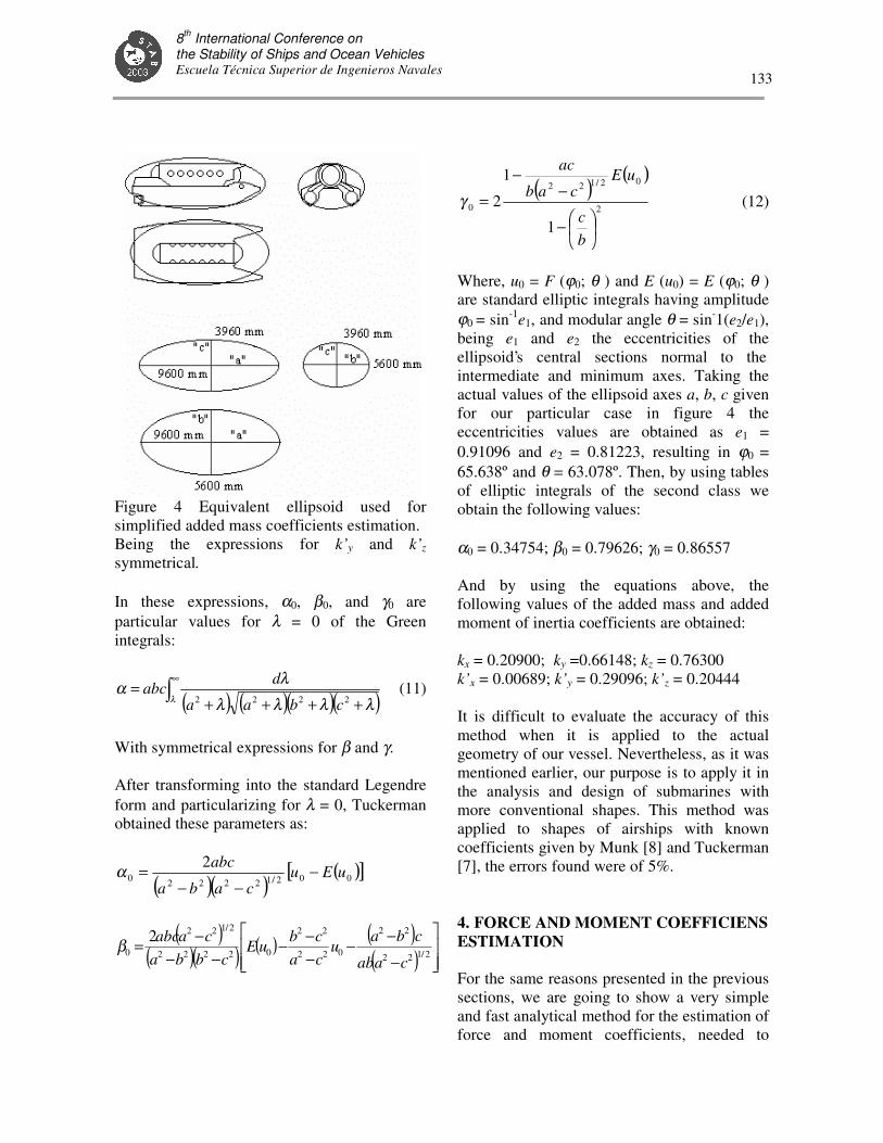
Figure 4 Equivalent ellipsoid used for simplified added mass coefficients estimation. Being the expressions for k’y and k’z symmetrical. In these expressions, α0, β0, and γ0 are particular values for λ = 0 of the Green integrals:

( ) ( )( )( )∫∞

++++=

λ λλλλλα

2222 cbaa

dabc (11)

With symmetrical expressions for β and γ. After transforming into the standard Legendre form and particularizing for λ = 0, Tuckerman obtained these parameters as:

( )( ) ( )[ ]002/1222202

uEucaba

abc −−−

=α

( )( )( ) ( ) ( )

( )

−

−−−−−

−−−=

2/122

22

022

22

02222

2/122

02

caab

cbau

cacb

uEcbba

caabcβ

( ) ( )2

02/122

0

1

1

2

−

−−

=

bc

uEcab

ac

γ (12)

Where, u0 = F (ϕ0; θ ) and E (u0) = E (ϕ0; θ ) are standard elliptic integrals having amplitude ϕ0 = sin-1e1, and modular angle θ = sin-1(e2/e1), being e1 and e2 the eccentricities of the ellipsoid’s central sections normal to the intermediate and minimum axes. Taking the actual values of the ellipsoid axes a, b, c given for our particular case in figure 4 the eccentricities values are obtained as e1 = 0.91096 and e2 = 0.81223, resulting in ϕ0 = 65.638º and θ = 63.078º. Then, by using tables of elliptic integrals of the second class we obtain the following values: α0 = 0.34754; β0 = 0.79626; γ0 = 0.86557 And by using the equations above, the following values of the added mass and added moment of inertia coefficients are obtained: kx = 0.20900; ky =0.66148; kz = 0.76300 k’x = 0.00689; k’y = 0.29096; k’z = 0.20444 It is difficult to evaluate the accuracy of this method when it is applied to the actual geometry of our vessel. Nevertheless, as it was mentioned earlier, our purpose is to apply it in the analysis and design of submarines with more conventional shapes. This method was applied to shapes of airships with known coefficients given by Munk [8] and Tuckerman [7], the errors found were of 5%. 4. FORCE AND MOMENT COEFFICIENS ESTIMATION For the same reasons presented in the previous sections, we are going to show a very simple and fast analytical method for the estimation of force and moment coefficients, needed to



calculate the hydrodynamic reactions exerted on the submarine. Some early potential methods developed for airships, such as the ones by Munk [8] and Laitone [9] did not provide satisfactory results because they did not take in account the viscous and turbulent effects which are very important in the aft. The model by Hopkins [10] is probably the simplest one taking into account these effects and providing satisfactory enough results. This semi empirical method determines the lift, drag and pitch moment of bodies of revolution by using their added mass coefficients. Thus, to use it we must transform the equivalent ellipsoid of our vehicle into an ellipsoid of revolution. Then, it will be considered that in a large fore part of the body the flow is governed by potential theory, while in a smaller aft part viscous and turbulent effects are dominant. To account for all this, a conical surface is added as an after body as shown in figure 5. This after-body cone is tangent to the ellipsoid in a circle placed at a distance x1 from the front end but it is assumed that the potential flow extends a bit further back of this place to a distance x0. The force and moment coefficients result from the following expressions:

( ) ( )

( )

( )

( )dxCr

Vdx

dxdS

V

kkC

dxCrV

dxdxdS

V

kkC

dxxxCr

Vdxxx

dxdS

Vkk

C

L

xdc

x

D

L

xdc

x

L

L

xmdc

x

mMy

∫∫

∫∫

∫

∫

⋅⋅⋅⋅⋅+⋅⋅⋅⋅−=

⋅⋅⋅⋅⋅+⋅⋅⋅⋅−=

⋅−⋅⋅⋅

⋅⋅+⋅−⋅⋅⋅⋅−=

0

0

0

0

0

0

32

3

032

212

32

2

032

12

2

0

12

22

22

22

ηαα

ηαα

η

αα

(13) Where k1 and k2 are the added mass coefficients in the longitudinal and transversal directions, L is the vehicle’s total length, S is the cross sectional area, which is a function of x, α is the angle of attack, xm is the coordinate of the point where the moments are taken, η is the ratio between the drag coefficient of a cylinder with the same thickness as the ellipsoid and the drag coefficient of an infinite cylinder, Cdc is the drag coefficient of an infinite cylinder, and r is the local radius. According to Hopkins [10], the coordinate x1 is taken where dS/dx reaches its largest negative value, and x0 is given by the empirical correlation:

Figure 5 Equivalent ellipsoid and conical after-body used for simplified force and moment coefficients estimation


135

Lx

Lx 10 527.0378.0 += (14)

The drag proportionality factor η is given as a function of the ratio n between both ellipsoids’ axes by the empirical correlation:

12.0

220

= nη (15)

This correlation has been obtained by fitting a graph by Hopkins [10] where different experimental results are plotted. Applying all these expressions to the actual geometry of the ellipsoid fitting our submarine, the following values of the coefficient are obtained:

32

2

2

04539.034798.0

04539.034798.0

07026.039233.0

αααα

αα

⋅+⋅=

⋅+⋅=

⋅−⋅=

D

L

My

C

C

C

(16)

Taking into account the symmetry of this ellipsoid the values of the other coefficients are obtained from these:

0

04539.034798.0

07026.039233.02

2

=

⋅+⋅=

⋅−⋅=

Mx

Q

Mz

C

C

C

ββββ

(17)

From these values we can immediately gather that the submarine defined as before without control surfaces is unstable because CMy is positive for any α < 5.58 rad. As it was the case for the added mass coefficients, the accuracy of this method could be compromised when applied to the complex geometry of our catamaran. However, comparing our method with the experimental results on airships giving by Hopkins, the calculated values result to be 17% lower than the experiments. Some other comparisons were

performed with experiments made in deceleration test of airships by Thompson and Kirschbaum [14] giving calculated values 18% lower than experiments. 5. FORCES AND MOMENTS EXERTED BY THE CONTROL SURFACES Modeling forces and moments exerted by the fins and rudders is a fundamental task in designing the control system for this type of vehicles. In general, considering these forces as a result of hydrodynamic reactions, they can be expressed as:

( )τδξ ++⋅⋅⋅⋅= pRudderRudderLRudder SCF 2.2

1 V

(18) Where the incidence angle of the flow reaching the rudder is taken as the sum of the general incidence angle ξ in the plane normal to the rudder, plus the deflection of the rudder δ, plus the deviation angle τ due to the vehicle’s angular velocity. The general incidence angle ξ in the plane normal to the rudder is equal to the angle of attack α for the horizontal control planes, and is equal to the side slip angle β for the vertical ones. The deviation angle τ due to the vehicle’s angular velocity for a horizontal control surface can be obtained as:

xVV Rudderz xq−

=τ (19)

And for vertical control surfaces:

xV

V Ruddery xr+=τ (20)

To obtain the moments exerted by the control surface’s reactions on the vehicle’s center of gravity it is sufficient to multiply de force FRudder by the distance xRudder. In any case all these forces and moments are of the



hydrodynamic type, thus the above used expressions are only valid in a reference coordinate system oriented with the local flow velocity. In order to transform them into a body-fixed system, they must be multiplied by a matrix similar to the Lbw defined earlier but having the angles α and β added to their corresponding deviation angle τ. 6. SIMULATION The described equations of motion of the vehicle, as well as the estimated forces, moments, added mass, and added inertia coefficients and the appropriate transformation matrixes have been implemented in a simulator by using Simulink and the Matlab working space. This simulator was used first to perform the stability studies in the present work and, in addition, it has been used within the evolutionary control design system mentioned earlier and presented by Lamas et Al [11]. The dynamic iteration loop required was of 10-4, the time step was of 10-2 and the sampling time was of 10-3. To have a validation of the performance of this simulator, it was applied to the REMUS autonomous underwater vehicle by Prestero [12]. The characteristics of this vehicle were implemented in our simulator and the results obtained were found to be in

agreement with the data published by Prestero, as shown in figure 6. The differences observed arise from the fact that in Prestero’s case a controller is implemented while in our simulation no controller is present, nevertheless the main behavior characteristics are captured.

Figure 7 The three different configuration of rudders used.

Figure 6 REMUS simulations by Prestero (above) and by our model (below).


137

Figure 8. Results of moments and angle evolution for the three models with 100 N of thrust, rudders fixed in a neutral position and 2% more buoyancy than weight

Three different models of our vehicle corresponding to three configurations of the control planes were modeled, as shown in figure 7. The first and second models include a single elevation rudder placed in the rear and in the middle part respectively, while the third model has two elevation rudders as a

combination of the other two. Different simulations were performed for each one of these models after varying the thrust applied and the rudders positions. In all cases the catamaran behavior results unstable. As an example, figure 8 shows the results for the three models with 100 N of thrust, being their



Figure 9 Results of moments and angle evolution for model 1 with 5000 N of thrust, rudders fixed in a neutral position and 2% more buoyancy than weight. buoyancy 2% larger than their weight, and having their rudders fixed in a neutral position. In all cases, in addition to the hydrodynamic moments, a restoring moment between buoyancy and weight appears for any pitch angle different from zero. These restoring moments are the main cause of the oscillations appearing in all cases a short time after the departure from the initial equilibrium position. Except for model 1 these oscillations diverge, but even in model 1 these oscillations appear around a position that is different from the original one. Figure 9 shows the results for model 1 with the same conditions as before but having a thrust of 5000 N. We can see that the solution becomes even more unstable.

In order to quantify this intrinsic instability of the vehicle we have resorted to the definition of two non dimensional parameters: the angular position instability parameter (ζ ) and the angular acceleration instability parameter (η):

2

00 V;

V

⋅=⋅

∆∆=

gq

gt&ηθζ (21)

Where V0 is the initial test velocity and ∆θ is the maximum value of the pitch, yaw or roll angles achieved during time ∆t. After these definitions it is clear that the larger these parameters are the larger the instability is.

Table1 Average values of the angular position instability parameter (ζ ) Thrust Model 1 Model 2 Model 3 100 N 0.4136188 0.4798711 0.490919666 5000 N 0.55383222 0.840444777 0.67224002

Table2 Average values of the angular acceleration instability parameter (η) Thrust Model 1 Model 2 Model 3 100 N 0.007827333 0.013238 0.01495422 5000 N 0.039818222 0.01782477 0.019825566


139

The average values of these parameters were obtained after running the simulator for the three models tested for different rudder positions ranging from -10 to 10 degrees. Tables 1 and 2 presents these average values. It is clear that model 1 is the least unstable, and model 3 the most unstable, and that the instability increases with thrust. The body of the submarine and the fore rudder contribute to increasing the instability, while the aft rudder decreases it. A wider variety of tests results can be found in Fernández Ibarz [13]. 7. CONCLUSIONS A general model and simulator to study the dynamics of submarines has been developed from scratch and implemented within the Simulink environment. This simulator has been complemented with some simple analytical methods to obtain forces, moments and added mass coefficients needed for the calculations. This simulator has been validated with different published data from several airships and a submarine and then it has been applied to the stability analysis of a submersible catamaran with three possible rudder configurations. The results prove that the vehicle is intrinsically unstable. 8. ACKNOWLEDGMENTS This work was partially supported by the FEDER through project PROTECAS N. 1FD1997-1262 MAR. 9. REFERENCES [1]. Brutzman, D. P. "A Virtual World for an Autonomous Underwater Vehicle" Naval Postgraduate School, Monterrey, California. December 1994.

[2]. Abkowitz, M. A. "Stability and Motion Control of Ocean Vehicles" MIT Press. Cambridge, Massachusetts. 1969. [3]. Coxon, P. J. "System Identification of Submarine Hydrodynamic Coefficients from Simple Full Scale Trials" Ph.D. Thesis, Department of Ocean Engineering, MIT. 1989. [4]. Feldman, J. "Revised Standard Submarine Equations of Motion". Technical report DTNSRDC/SPD-0393-09, David W. Taylor Naval Ship Research and Development Center (DTNSRDC), Bethesda Maryland, June 1979. [5]. Gertler, M. and Hagen, G. "Standard Equations of Motion for Submarine Simulation" Naval Ship Research and Development Center, Report 2510. 1976. [6]. Sahin I., Crane, J. and Watson, K. "Added Mass Coefficients for Submerged Bodies by a Low-Order Panel Method". Journal of Fluids Engineering, vol. 115, pags. 452-456. 1993. [7]. Tuckerman, L. B. "Inertia Factors of Ellipsoid for Use in Airship Design". Report NACA Nº.210. National Advisory Committee for Aeronautics. 1926. [8]. Munk, M. M. "The Aerodynamic Forces on Airship Hulls". Report NACA Nº.184. National Advisory Committee for Aeronautics. 1924. [9]. Laitone, E. V. "The Linearized Subsonic and Supersonic Flow about Inclined Bodies of Revolution". Jour. Aero. Sci. Vol.14 nº 11, pp. 631-642. 1947. [10]. Hopkins, E. J. "A Semiempirical Method for Calculating the Pitching Moment of Bodies of Revolution at Low Mach Numbers". Ames Aeronautical Laboratory Moffett Field, California. Research Memorandum RM A51C14. 1954.



[11]. Lamas, A., Fernández Ibarz, J. & Duro, R. "Diseño evolutivo de un control neuronal para catamaranes submarinos". II Congreso Español sobre Metaheurísticas, Algoritmos Evolutivos y Bioinspirados, MAEB2003. Feb 2003 [12]. Prestero, T. "Verification of a Six-Degree of Freedom Simulation Model for the REMUS Autonomous Underwater Vehicle". Ph.D. Thesis, Department of Ocean Engineering, MIT, and Department of Ocean Engineering, WHOI. 2001.

[13]. Fernández Ibarz, J. “Modelo de simulación y control dinámico para un catamarán submarino con seis grados de libertad”. PhD Thesis, Universidade da Coruña, Spain. April 2003. [14]. Thompson, F. L. and Kirschbaum H.W. "The Drag Characteristics of Several Airships Determined by Deceleration Tests". Report NACA Nº.397. National Advisory Committee for Aeronautics. 1931.

8 international conference on the stability of ships...

Documents