8 fast learning algorithms - freie universitätpage.mi.fu-berlin.de/rojas/neural/chapter/k8.pdf ·...

R. Rojas: Neural Networks, Springer-Verlag, Berlin, 1996

8

Fast Learning Algorithms

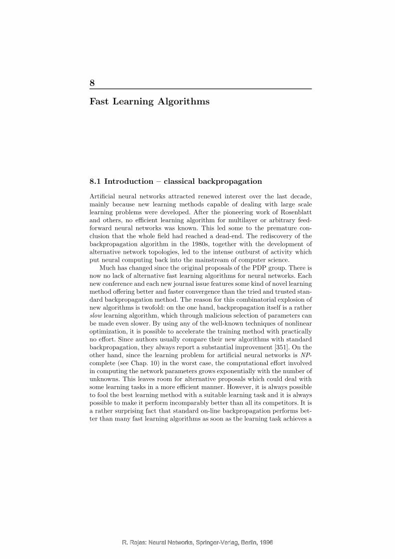
8.1 Introduction – classical backpropagation

Artificial neural networks attracted renewed interest over the last decade,mainly because new learning methods capable of dealing with large scalelearning problems were developed. After the pioneering work of Rosenblattand others, no efficient learning algorithm for multilayer or arbitrary feed-forward neural networks was known. This led some to the premature con-clusion that the whole field had reached a dead-end. The rediscovery of thebackpropagation algorithm in the 1980s, together with the development ofalternative network topologies, led to the intense outburst of activity whichput neural computing back into the mainstream of computer science.

Much has changed since the original proposals of the PDP group. There isnow no lack of alternative fast learning algorithms for neural networks. Eachnew conference and each new journal issue features some kind of novel learningmethod offering better and faster convergence than the tried and trusted stan-dard backpropagation method. The reason for this combinatorial explosion ofnew algorithms is twofold: on the one hand, backpropagation itself is a ratherslow learning algorithm, which through malicious selection of parameters canbe made even slower. By using any of the well-known techniques of nonlinearoptimization, it is possible to accelerate the training method with practicallyno effort. Since authors usually compare their new algorithms with standardbackpropagation, they always report a substantial improvement [351]. On theother hand, since the learning problem for artificial neural networks is NP-complete (see Chap. 10) in the worst case, the computational effort involvedin computing the network parameters grows exponentially with the number ofunknowns. This leaves room for alternative proposals which could deal withsome learning tasks in a more efficient manner. However, it is always possibleto fool the best learning method with a suitable learning task and it is alwayspossible to make it perform incomparably better than all its competitors. It isa rather surprising fact that standard on-line backpropagation performs bet-ter than many fast learning algorithms as soon as the learning task achieves a

R. Rojas: Neural Networks, Springer-Verlag, Berlin, 1996R. Rojas: Neural Networks, Springer-Verlag, Berlin, 1996


186 8 Fast Learning Algorithms

realistic level of complexity and when the size of the training set goes beyonda critical threshold [391].

In this chapter we try to introduce some order into the burgeoning field offast learning algorithms for neural networks. We show the essential character-istics of the proposed methods, the fundamental alternatives open to anyonewishing to improve traditional backpropagation and the similarities and dif-ferences between the different techniques. Our analysis will be restricted tothose algorithms which deal with a fixed network topology. One of the lessonslearned over the past years is that significant improvements in the approxi-mation capabilities of neural networks will only be obtained through the useof modularized networks. In the future, more complex learning algorithms willdeal not only with the problem of determining the network parameters, butalso with the problem of adapting the network topology. Algorithms of thistype already in existence fall beyond the scope of this chapter.

8.1.1 Backpropagation with momentum

Before reviewing some of the variations and improvements which have beenproposed to accelerate the learning process in neural networks, we briefly dis-cuss the problems involved in trying to minimize the error function usinggradient descent. Therefore, we first describe a simple modification of back-propagation called backpropagation with momentum, and then look at theform of the iteration path in weight space.

w

w

(a) (b)

iteration path

1

2w

2

w1

Fig. 8.1. Backpropagation without (a) or with (b) momentum term

When the minimum of the error function for a given learning task lies in anarrow “valley”, following the gradient direction can lead to wide oscillationsof the search process. Figure 8.1 shows an example for a network with justtwo weights w1 and w2. The best strategy in this case is to orient the searchtowards the center of the valley, but the form of the error function is suchthat the gradient does not point in this direction. A simple solution is to



8.1 Introduction – classical backpropagation 187

introduce a momentum term. The gradient of the error function is computedfor each new combination of weights, but instead of just following the negativegradient direction a weighted average of the current gradient and the previouscorrection direction is computed at each step. Theoretically, this approachshould provide the search process with a kind of inertia and could help toavoid excessive oscillations in narrow valleys of the error function.

As explained in the previous chapter, in standard backpropagation theinput-output patterns are fed into the network and the error function E isdetermined at the output. When using backpropagation with momentum in anetwork with n different weights w1, w2, . . . , wn, the i-th correction for weightwk is given by

∆wk(i) = −γ ∂E∂wk

+ α∆wk(i− 1),

where γ and α are the learning and momentum rate respectively. Normally, weare interested in accelerating convergence to a minimum of the error function,and this can be done by increasing the learning rate up to an optimal value.Several fast learning algorithms for neural networks work by trying to findthe best value of γ which still guarantees convergence. Introduction of themomentum rate allows the attenuation of oscillations in the iteration process.

The adjustment of both learning parameters to obtain the best possibleconvergence is normally done by trial and error or even by some kind of ran-dom search [389]. Since the optimal parameters are highly dependent on thelearning task, no general strategy has been developed to deal with this prob-lem. Therefore, in the following we show the trade-offs involved in choosinga specific learning and momentum rate, and the kind of oscillating behav-ior which can be observed with the backpropagation feedback rule and largemomentum rates. We show that they are necessary when the optimal sizeof the learning step is unknown and the form of the error function is highlydegenerate.

The linear associator

Let us first consider the case of a linear associator, that is, a single comput-ing element with associated weights w1, w2, . . . , wn and which for the inputx1, x2, . . . , xn produces w1x1 + · · ·+wnxn as output, as shown in Figure 8.2.

x1

x2

xn

w1

wn

wixii =1

n

Σ+w2

Fig. 8.2. Linear associator




The input-output patterns in the training set are the p ordered pairs(x1, y1), . . . , (xp, yp), whereby the input patterns are row vectors of dimensionn and the output patterns are scalars. The weights of the linear associator canbe ordered in an n-dimensional column vector w and the learning task consistsof finding the w that minimizes the quadratic error

E =

n∑

i=1

‖xi ·w − yi‖2.

By defining a p × m matrix X whose rows are the vectors x1, . . . ,xp and acolumn vector y whose elements are the scalars y1, . . . , yp, the learning taskreduces to the minimization of

E = ‖Xw− y‖2

= (Xw − y)T(Xw − y)

= wT(XTX)w − 2yTXw + yTy.

Since this is a quadratic function, the minimum can be found using gradientdescent.

The quadratic function E can be thought of as a paraboloid in m-dimensional space. The lengths of its principal axes are determined by themagnitude of the eigenvalues of the correlation matrix XTX. Gradient de-scent is most effective when the principal axes of the quadratic form are all ofthe same length. In this case the gradient vector points directly towards theminimum of the error function. When the axes of the paraboloid are of verydifferent sizes, the gradient direction can lead to oscillations in the iterationprocess as shown in Figure 8.1.

Let us consider the simple case of the quadratic function ax2 + by2. Gra-dient descent with momentum yields the iteration rule

∆x(i) = −2γax+ α∆x(i − 1)

in the x direction and

∆y(i) = −2γbx+ α∆y(i− 1)

in the y direction. An optimal parameter combination in the x direction isγ = 1/2a and α = 0. In the y direction the optimal combination is γ = 1/2band α = 0. Since iteration proceeds with a single γ value, we have to finda compromise between these two options. Intuitively, if the momentum termis zero, an intermediate γ should do best. Figure 8.3 shows the number ofiterations needed to find the minimum of the error function to a given precisionas a function of γ, when a = 0.9 and b = 0.5. The optimal value for γ is theone found at the intersection of the two curves and is γ = 0.7. The globaloptimal γ is larger than the optimal γ in the x direction and smaller than theoptimal γ in the y direction. This means that there will be some oscillations




best commongamma

numberof iterations

γγ1 2

x dimension

y dimension

Fig. 8.3. Optimal γ in the two-dimensional case

in the y direction and slow convergence in the x direction, but this is the bestpossible compromise. It is obvious that in the n-dimensional case we couldhave oscillations in some of the principal directions and slow convergence inothers. A simple strategy used by some fast learning algorithms to avoid theseproblems consists of using a different learning rate for each weight, that is, adifferent γ for each direction in weight space [217].

Minimizing oscillations

Since the lengths of the principal axes of the error function are given by theeigenvalues of the correlation matrix XTX, and since one of these eigenvaluescould be much larger than the others, the range of possible values for γ reducesaccordingly. Nevertheless, a very small γ and the oscillations it produces canbe neutralized by increasing the momentum rate. We proceed to a detaileddiscussion of the one-dimensional case, which provides us with the necessaryinsight for the more complex multidimensional case.

In the one-dimensional case, that is, when minimizing functions of typekx2, the optimal learning rate is given by γ = 1/2k. The rate γ = 1/k pro-duces an oscillation between the initial point x0 and −x0. Any γ greaterthan 2/k leads to an “explosion” of the iteration process. Figure 8.4 showsthe main regions for parameter combinations of γ and the momentum rateα. These regions were determined by iterating in the one-dimensional caseand integrating the length of the iteration path. Parameter combinations inthe divergence region lead to divergence of the iteration process. Parametercombinations in the boundary between regions lead to stable oscillations.




divergence

zone

convergence

zone

optimal combinations

of alpha and gamma

divergence

zone

0 10,5

Momentum rate

Learning

rate

1

2k

1

k

3

2k

2

k

Fig. 8.4. Convergence zone for combinations of γ and α

Figure 8.4 shows some interesting facts. Any value of γ greater than fourtimes the constant 1/2k cannot be balanced with any value of α. Values ofα greater than 1 are prohibited since they lead to a geometric explosion ofthe iteration process. Any value of γ between the explosion threshold 1/k and2/k can lead to convergence if a large enough α is selected. For any given γbetween 1/k and 2/k there are two points at which the iteration process fallsin a stable oscillation, namely at the boundaries between regions. For valuesof γ under the optimal value 1/2k, the convergence speed is optimal for aunique α. The optimal combinations of α and γ are the ones represented bythe jagged line in the diagram.

The more interesting message we get from Figure 8.4 is the following:in the case where in some direction in weight space the principal axis ofthe error function is very small compared to another axis, we should try toachieve a compromise by adjusting the momentum rate in such a way thatthe directions in which the algorithm oscillates become less oscillating and thedirections with slow convergence improve their convergence speed. Obviouslywhen dealing with n axes in weight space, this compromise could be dominatedby a single direction.




Critical parameter combinations

Backpropagation is used in those cases in which we do not have an analyticexpression of the error function to be optimized. A learning rate γ has to bechosen without any previous knowledge of the correlation matrix of the input.In on-line learning the training patterns are not always defined in advance,and are generated one by one. A conservative approach is to minimize the riskby choosing a very small learning rate. In this case backpropagation can betrapped in a local minimum of a nonlinear error function. The learning rateshould then be increased.

Fig. 8.5. Paths in weight space for backpropagation learning (linear associators).The minimum of the error function is located at the origin.

In the case of a correlation matrix XTX with some very large eigenval-ues, a given choice of γ could lead to divergence in the associated directionin weight space (assuming for simplicity that the principal directions of thequadratic form are aligned with the coordinate axis). Let us assume that theselected γ is near to the explosion point 2/k found in the one-dimensional caseand shown in Figure 8.4. In this case only values of the momentum rate nearto one can guarantee convergence, but oscillations in some of the directionsin weight space can become synchronized. The result is oscillating paths inweight space, reminiscent of Lissajou’s figures. Figure 8.5 shows some pathsin a two-dimensional weight space for several linear associators trained with




momentum rates close to one and different γ values. In some cases the tra-jectories lead to convergence after several thousand iterations. In others amomentum rate equal to one precludes convergence of the iteration process.

Adjustment of the learning and momentum rate in the nonlinear case iseven more difficult than in the linear case, because there is no fast explosionof the iteration process. In the quadratic case, whenever the learning rateis excessively large, the iteration process leads rapidly to an overflow whichalerts the programmer to the fact that the step size should be reduced. In thenonlinear case the output of the network and the error function are boundedand no overflow occurs. In regions far from local minima the gradient of theerror function becomes almost zero as do the weight adjustments. The diver-gence regions of the quadratic case can now become oscillatory regions. Inthis case, even as step sizes increase, the iteration returns to the convex partof the error function.

0.25

0.0

error

weightupdates

iterations

Fig. 8.6. Bounded nonlinear error function and the result of several iterations

Figure 8.6 shows the possible shape of the error function for a linear as-sociator with sigmoidal output and the associated oscillation process for thiskind of error function in the one-dimensional case. The jagged form of theiteration curve is reminiscent of the kind of learning curves shown in manypapers about learning in nonlinear neural networks. Although in the quadraticcase only large momentum rates lead to oscillations, in the nonlinear case anexcessively large γ can also produce oscillations even when no momentum rateis present.

Researchers in the field of neural networks should be concerned not onlywith the possibility of getting stuck in local minima of the error function whenlearning rates are too small, but also with the possibility of falling into the os-cillatory traps of backpropagation when the learning rate is too big. Learningalgorithms should try to balance the speedup they are attempting to obtainwith the risk of divergence involved in doing so. Two different kinds of remedyare available: a) adaptive learning rates and b) statistical preprocessing of thelearning set which is done to decorrelate the input patterns, thus avoiding thenegative effect of excessively large eigenvalues of the correlation matrix.




8.1.2 The fractal geometry of backpropagation

It is empirically known that standard backpropagation is very sensitive tothe initial learning rate chosen for a given learning task. In this section weexamine the shape of the iteration path for the training of a linear associatorusing on-line backpropagation. We show that the path is a fractal in weightspace. The specific form depends on the learning rate chosen, but there isa threshold value for which the attractor of the iteration path is dense in aregion of weight space around a local minimum of the error function. Thisresult also yields a deeper insight into the mechanics of the iteration processin the nonlinear case.

The Gauss–Jacobi and Gauss–Seidel methods and backpropagation

Backpropagation can be performed in batch or on-line mode, that is, by updat-ing the network weights once after each presentation of the complete trainingset or immediately after each pattern presentation. In general, on-line back-propagation does not converge to a single point in weight space, but oscillatesaround the minimum of the error function. The expected value of the devia-tion from the minimum depends on the size of the learning step being used. Inthis section we show that although the iteration process can fail to convergefor some choices of learning rate, the iteration path for on-line learning is notjust random noise, but possesses some structure and is indeed a fractal. Thisis rather surprising, because if the training patterns are selected randomly,one would expect a random iteration path. As we will see in what follows, itis easy to show that on-line backpropagation, in the case of linear associators,defines an Iterated Function System of the same type as the ones popular-ized by Barnsley [42]. This is sufficient proof that the iteration path has afractal structure. To illustrate this fact we provide some computer-generatedgraphics.

First of all we need a visualization of the way off-line and on-line back-propagation approach the minimum of the error function. To simplify thediscussion consider a linear associator with just two input lines (and thus twoweights w1 and w2). Assume that three input-output patterns are given sothat the equations to be satisfied are:

x11w1 + x1

2w2 = y1 (8.1)

x21w1 + x2

2w2 = y2 (8.2)

x31w1 + x3

2w2 = y3 (8.3)

These three equations define three lines in weight space and we look for thecombination of w1 and w2 which satisfies all three simultaneously. If the threelines intersect at the same point, we can compute the solution using Gausselimination. If the three lines do not intersect, no exact solution exists butwe can ask for the combination of w1 and w2 which minimizes the quadratic




error. This is the point inside the triangle shown in Figure 8.7, which has theminimal cumulative quadratic distance to the three sides of the triangle.

P

Fig. 8.7. Three linear constraints in weight space

Now for the interesting part: the point of intersection of linear equationscan be found by linear algebraic methods such as the Gauss–Jacobi or theGauss–Seidel method. Figure 8.8 shows how they work. If we are looking forthe intersection of two lines, the Gauss–Jacobi method starts at some point insearch space and projects this point in the directions of the axes on to the twolines considered in the example. The x-coordinate of the horizontal projectionand the y-coordinate of the vertical projection define the next iteration point.It is not difficult to see that in the example this method converges to thepoint of intersection of the two lines. The Gauss–Seidel method deals witheach linear equation individually. It first projects in the x direction, then inthe y direction. Each projection is the new iteration point. This algorithmusually converges faster than the Gauss–Jacobi method [444].

Gauss-Jacobi iterations Gauss-Seidel iterations

Fig. 8.8. The Gauss–Jacobi and Gauss–Seidel methods

Off-line and on-line backpropagation are in a certain sense equivalent tothe Gauss–Jacobi and Gauss–Seidel methods. When on-line backpropagation




is used, the negative gradient of the error function is followed and this corre-sponds to following a line perpendicular to each one of the equations (8.1) to(8.3). In the case of the first input-output pattern, the error function is

1

2(x1

1w1 + x12w2 − y1)2

and the gradient (with respect to w1 and w2) is the vector

(x1, x2)

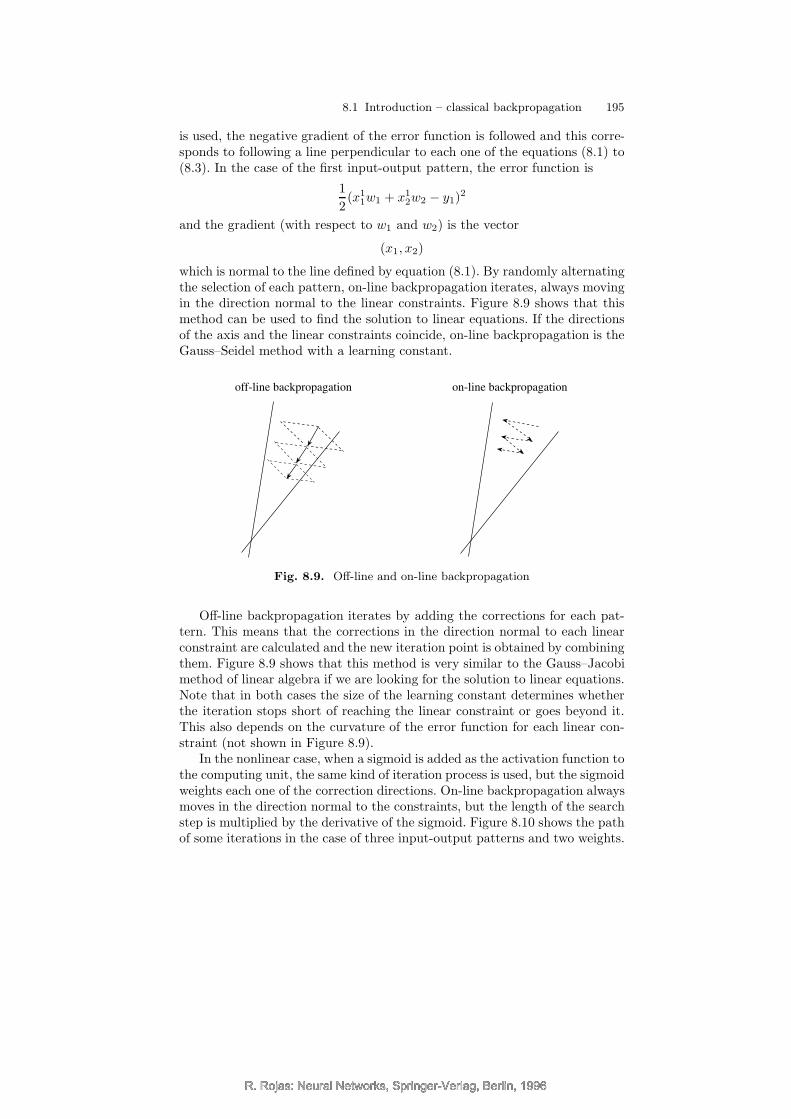
which is normal to the line defined by equation (8.1). By randomly alternatingthe selection of each pattern, on-line backpropagation iterates, always movingin the direction normal to the linear constraints. Figure 8.9 shows that thismethod can be used to find the solution to linear equations. If the directionsof the axis and the linear constraints coincide, on-line backpropagation is theGauss–Seidel method with a learning constant.

off-line backpropagation on-line backpropagation

Fig. 8.9. Off-line and on-line backpropagation

Off-line backpropagation iterates by adding the corrections for each pat-tern. This means that the corrections in the direction normal to each linearconstraint are calculated and the new iteration point is obtained by combiningthem. Figure 8.9 shows that this method is very similar to the Gauss–Jacobimethod of linear algebra if we are looking for the solution to linear equations.Note that in both cases the size of the learning constant determines whetherthe iteration stops short of reaching the linear constraint or goes beyond it.This also depends on the curvature of the error function for each linear con-straint (not shown in Figure 8.9).

In the nonlinear case, when a sigmoid is added as the activation function tothe computing unit, the same kind of iteration process is used, but the sigmoidweights each one of the correction directions. On-line backpropagation alwaysmoves in the direction normal to the constraints, but the length of the searchstep is multiplied by the derivative of the sigmoid. Figure 8.10 shows the pathof some iterations in the case of three input-output patterns and two weights.




Fig. 8.10. On-line backpropagation iterations for sigmoidal units

Iterated Function Systems

Barnsley has shown that a set of affine transformations in a metric spacecan produce fractal structures when applied repetitively to a compact subsetof points and its subsequent images. More specifically: an Iterated FunctionSystem (IFS) consists of a space of points X , a metric d defined in this space,and a set of affine contraction mappings hi : X → X, i = 1, . . . , N . Given anonvoid compact subset A0 of points of X , new image subsets are computedsuccessively according to the recursive formula

An+1 =

N⋃

j=1

hj(An), for n = 1, 2, . . . .

A theorem guarantees that the sequence {An} converges to a fixed point,which is called the attractor of the IFS. Moreover, the Collage Theorem guar-antees that given any nonvoid compact subset of X we can always find anIFS whose associated attractor can arbitrarily approximate the given subsetunder a suitable metric.

For the case of an n-dimensional space X , an affine transformation appliedto a point x = (x1, x2, . . . , xn) is defined by a matrix M and a vector t. Thetransformation is given by

x→Mx + t.

and is contractive if the determinant of M is smaller than one.It is easy to show that the attractor of the IFS can be approximated

by taking any point ao which belongs to the attractor and computing thesequence an, whereby

an+1 = hk(an),

and the affine transformation hk is selected randomly from the IFS. The infi-nite sequence {an} is a dense subset of the attractor. This means that we canproduce a good graphical approximation of the attractor of the IFS with thissimple randomized method. Since it is easy to approximate a point belongingto the attractor (by starting from the origin and iterating with the IFS a fixednumber of times), this provides us with the necessary initial point.




We now proceed to show that on-line backpropagation, in the case of alinear associator, defines a set of affine transformations which are applied inthe course of the learning process either randomly or in a fixed sequence. Theiteration path of the initial point is thus a fractal.

On-line Backpropagation and IFS

Consider a linear associator and the p n-dimensional patterns x1,x2, . . . ,xp.The symbol xj

i denotes the i-th coordinate of the j-th pattern. The targets fortraining are the p real values y1, y2, . . . , yp. We denote by w1, w2, . . . , wn theweights of the linear associator. In on-line backpropagation the error functionis determined for each individual pattern. For pattern j the error is

Ej =1

2(w1x

j1 + w2x

j2 + · · ·+ wnx

jn − yj)2.

The correction for each weight wi, i = 1, . . . , n, is given by

wi → wi − γxji (w1x

j1 + w2x

j2 + · · ·+ wnx

jn − yj),

where γ is the learning constant being used. This can be also written as

wi → wi − γ(w1xjix

j1 + w2x

jix

j2 + · · ·+ wnx

jix

jn)− γxj

iyj . (8.4)

Let Mj be the matrix with elements mik = xjix

jk for i, k = 1, . . . , n. Equa-

tion (8.4) can be rewritten in matrix form (considering all values of i) as

w→ Iw − γMjw− tj ,

where tj is the column vector with components xjiy

j for i = 1, . . . , n and I isthe identity matrix. We can rewrite the above expression as

w→ (I− γMj)w − tj .

This is an affine transformation, which maps the current point in weight spaceinto a new one. Note that each pattern in the training set defines a differentaffine transformation of the current point (w1, w2, . . . , wn).

In on-line backpropagation with a random selection of input patterns,the initial point in weight space is successively transformed in just the wayprescribed by a randomized IFS algorithm. This means that the sequence ofupdated weights approximates the attractor of the IFS defined by the inputpatterns, i.e., the iteration path in weight space is a fractal.

This result can be visualized in the following manner: given a point(w′

1, w′2, . . . , w

′n) in weight space, the square of the distance ` to the hyperplane

defined by the equation

w1xj1 + w2x

j2 + · · ·+ wnx

jn = yj




Fig. 8.11. Iteration paths in weight space for different learning rates

is given by

`2 =(w′

1xj1 + w′

2xj2 + · · ·+ w′

nxjn − yj)2

(xj1)

2 + · · ·+ (xjn)2

.

Comparing this expression with the updating step performed by on-linebackpropagation, we see that each backpropagation step amounts to displac-ing the current point in weight space in the direction normal to the hyperplanedefined by the input and target patterns. A learning rate γ with value

γ =1

(xj1)

2 + · · ·+ (xjn)2

(8.5)

produces exact learning of the j-th pattern, that is, the point in weight spaceis brought up to the hyperplane defined by the pattern. Any value of γ belowthis threshold displaces the iteration path just a fraction of the distance tothe hyperplane. The iteration path thus remains trapped in a certain regionof weight space near to the optimum.

Figure 8.11 shows a simple example in which three input-output patternsdefine three lines in a two-dimensional plane. Backpropagation for a linearassociator will find the point in the middle as the solution with the minimalerror for this task. Some combinations of learning rate, however, keep theiteration path a significant distance away from this point. The fractal structureof the iteration path is visible in the first three graphics. With γ = 0.25the fractal structure is obliterated by a dense approximation to the wholetriangular region. For values of γ under 0.25 the iteration path repeatedlycomes arbitrarily near to the local minimum of the error function.



8.2 Some simple improvements to backpropagation 199

It is clear that on-line backpropagation with random selection of the inputpatterns yields iteration dynamics equivalent to those of IFS. When the learn-ing constant is such that the affine transformations overlap, the iteration pathdensely covers a certain region of weight space around the local minimum ofthe error function. Practitioners know that they have to systematically re-duce the size of the learning step, because otherwise the error function beginsoscillating. In the case of linear associators and on-line backpropagation thismeans that the iteration path has gone fractal. Chaotic behavior of recurrentneural networks has been observed before [281], but in our case we are dealingwith very simple feed-forward networks which fall into a similar dynamic.

In the case of sigmoid units at the output, the error correction step isno longer equivalent to an affine transformation, but the updating step isvery similar. It can be shown that the error function for sigmoid units canapproximate a quadratic function for suitable parameter combinations. In thiscase the iteration dynamics will not differ appreciably from those discussed inthis chapter. Nonlinear updating steps should also produce fractal iterationpaths of a more complex nature.

8.2 Some simple improvements to backpropagation

Since learning in neural networks is an NP-complete problem and since tradi-tional gradient descent methods are rather slow, many alternatives have beentried in order to accelerate convergence. Some of the proposed methods aremutually compatible and a combination of them normally works better thaneach method alone [340]. But apart from the learning algorithm, the basicpoint to consider before training a neural network is where to start the itera-tive learning process. This has led to an analysis of the best possible weightinitialization strategies and their effect on the convergence speed of learning[328].

8.2.1 Initial weight selection

A well-known initialization heuristic for a feed-forward network with sigmoidalunits is to select its weights with uniform probability from an interval [−α, α].The zero mean of the weights leads to an expected zero value of the total inputto each node in the network. Since the derivative of the sigmoid at each nodereaches its maximum value of 1/4 with exactly this input, this should leadin principle to a larger backpropagated error and to more significant weightupdates when training starts. However, if the weights in the networks arevery small (or all zero) the backpropagated error from the output to thehidden layer is also very small (or zero) and practically no weight adjustmenttakes place between input and hidden layer. Very small values of α paralyzelearning, whereas very large values can lead to saturation of the nodes in thenetwork and to flat zones of the error function in which, again, learning is very




slow. Learning then stops at a suboptimal local minimum [277]. Therefore itis natural to ask what is the best range of values for α in terms of the learningspeed of the network.

Some authors have conducted empirical comparisons of the values for αand have found a range in which convergence is best [445]. The main problemwith these results is that they were obtained from a limited set of exam-ples and the relation between learning step and weight initialization was notconsidered. Others have studied the percentage of nodes in a network whichbecome paralyzed during training and have sought to minimize it with the“best” α [113]. Their empirical results show, nevertheless, that there is not asingle α which works best, but a very broad range of values with basically thesame convergence efficiency.

Maximizing the derivatives at the nodes

Let us first consider the case of an output node. If n different edges with asso-ciated weights w1, w2, . . . , wn point to this node, then after selecting weightswith uniform probability from the interval [−α, α], the expected total inputto the node is ⟨

n∑

i=1

wixi

⟩

= 0

where x1, x2, . . . , xn are the input values transported through each edge. Wehave assumed that these inputs and the initial weights are not correlated. Bythe law of large numbers we can also assume that the total input to the nodehas a Gaussian distribution Numerical integration shows that the expectedvalue of the derivative is a decreasing function of the standard deviation σ.The expected value falls slowly with an increase of the variance. For σ = 0the expected value is 0.25 and for σ = 4 it is still 0.12, that is, almost half asbig.

The variance of the total input to a node is

σ2 = E((n∑

i=1

wixi)2)− E((

n∑

i=1

wixi))2 =

n∑

i=1

E(w2i )E(x2

i ),

since inputs and weights are uncorrelated. For binary vectors we have E(x2i ) =

1/3 and the above equation simplifies to

σ =1

3

√nα.

If n = 100, selecting weights randomly from the interval [−1.2, 1.2] leads to avariance of 4 at the input of a node with 100 connections and to an expectedvalue of the derivative equal to 0.12.

Therefore in small networks, in which the maximum input to each nodecomes from fewer than 100 edges, the expected value of the derivative is notvery sensitive to the width α of the random interval, when α is small enough.




Maximizing the backpropagated error

In order to make corrections to the weights in the first block of weights (thosebetween input and hidden layer) easier, the backpropagated error should be aslarge as possible. Very small weights between hidden and output nodes lead toa very small backpropagated error, and this in turn to insufficient correctionsto the weights. In a network with m nodes in the hidden layer and k nodesin the output layer, each hidden node h receives a backpropagated input δhfrom the k output nodes, equal to

δh =

k∑

i=1

whis′iδ

0i ,

where the weights whi, i = 1, . . . , k, are the ones associated with the edgesfrom hidden node h to output node i, s′i is the sigmoid’s derivative at theoutput node i, and δ0i is the difference between output and target also at thisnode.

alpha0.0

0.25

derivative's magnitude

backpropagated error

geometric mean

Fig. 8.12. Expected values of the backpropagated error and the sigmoid’s derivative

After initialization of the network’s weights the expected value of δh is zero.In the first phase of learning we are interested in breaking the symmetry of thehidden nodes. They should specialize in the recognition of different featuresof the input. By making the variance of the backpropagated error larger, eachhidden node gets a greater chance of pulling apart from its neighbors. Theabove equation shows that by making the initialization interval [−α, α] wider,two contradictory forces come into play. On the one hand, the variance ofthe weights becomes larger, but on the other hand, the expected value of thederivative s′k becomes lower. We would like to make δh as large as possible,but without making s′i too low, since weight corrections in the second blockof weights are proportional to s′i. Figure 8.12 shows the expected values ofthe derivative at the output nodes, the expected value of the backpropagated




error for the hidden nodes as a function of α, and the geometric mean of bothvalues. The data in the figure was obtained from Monte Carlo trials, assuminga constant expected value of δ0i . Forty hidden and one output unit were used.

The figure shows, again, that the expected value of the sigmoid’s derivativefalls slowly with an increasing α, but the value of the backpropagated erroris sensitive to small values of α. In the case shown in the figure, any possiblechoice of α between 0.5 and 1.5 should lead to virtually the same performance.This explains the flat region of possible values for α found in the experimentspublished in [113] and [445]. Consequently, the best values for α depend on theexact number of input, hidden, and output units, but the learning algorithmshould not be very sensitive to the exact α chosen from a certain range ofvalues.

8.2.2 Clipped derivatives and offset term

One of the factors which leads to slow convergence of gradient descent methodsis the small absolute value of the partial derivatives of the error functioncomputed by backpropagation. The derivatives of the sigmoid stored at thecomputing units can easily approach values near to zero and since severalof them can be multiplied in the backpropagation step, the length of thegradient can become too small. A solution to this problem is clipping thederivative of the sigmoid, so that it can never become smaller than a predefinedvalue. We could demand, for example, that s′(x) ≥ 0.01. In this case the“derivatives” stored in the computing units do not correspond exactly to theactual derivative of the sigmoid (except in the regions where the derivative isnot too small). However, the partial derivatives have the correct sign and thegradient direction is not significantly affected.

It is also possible to add a small constant ε to the derivative and uses′(x)+ε for the backpropagation step. The net effect of an offset value for thesigmoid’s derivative is to pull the iteration process out of flat regions of theerror function. Once this has happened, backpropagation continues iteratingwith the exact gradient direction. It has been shown in many different learningexperiments that this kind of heuristic, proposed by Fahlman [130], amongothers, can contribute significantly to accelerate several different variants ofthe standard backpropagation method [340]. Note that the offset term can beimplemented very easily when the sigmoid is not computed at the nodes butonly read from a table of function values. The table of derivatives can combineclipping of the sigmoid values with the addition of an offset term, to enhancethe values used in the backpropagation step.

8.2.3 Reducing the number of floating-point operations

Backpropagation is an expensive algorithm because a straightforward imple-mentation is based on floating-point operations. Since all values between 0and 1 are used, problems of precision and stability arise which are normally




avoided by using 32-bit or 64-bit floating-point arithmetic. There are severalpossibilities to reduce the number of floating-point operations needed.

Avoiding the computation of the squashing function

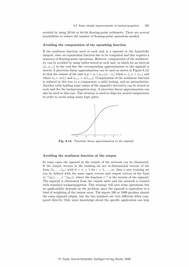
If the nonlinear function used at each unit is a sigmoid or the hyperbolictangent, then an exponential function has to be computed and this requires asequence of floating-point operations. However, computation of the nonlinear-ity can be avoided by using tables stored at each unit, in which for an interval[xi, xi+1] in the real line the corresponding approximation to the sigmoid isstored. A piecewise linear approximation can be used as shown in Figure 8.13,so that the output of the unit is y = ai +ai+1(x−xi) when xi ≤ x < xi+1 andwhere a1 = s(xi) and ai+1 = s(xi+1). Computation of the nonlinear functionis reduced in this way to a comparison, a table lookup, and an interpolation.Another table holding some values of the sigmoid’s derivative can be stored ateach unit for the backpropagation step. A piecewise linear approximation canalso be used in this case. This strategy is used in chips for neural computationin order to avoid using many logic gates.

-4 -2 0 2 4x

1

Fig. 8.13. Piecewise linear approximation to the sigmoid

Avoiding the nonlinear function at the output

In some cases the sigmoid at the output of the network can be eliminated.If the output vectors in the training set are m-dimensional vectors of theform (t1, . . . , tm) with 0 < ti < 1 for i = 1, . . . ,m, then a new training setcan be defined with the same input vectors and output vectors of the form(s−1(y1), . . . , s

−1(ym)), where the function s−1 is the inverse of the sigmoid.The sigmoid is eliminated from the output units and the network is trainedwith standard backpropagation. This strategy will save some operations butits applicability depends on the problem, since the sigmoid is equivalent to akind of weighting of the output error. The inputs 100 or 1000 produce almostthe same sigmoid output, but the two numbers are very different when com-pared directly. Only more knowledge about the specific application can help




to decide if the nonlinearity at the output can be eliminated (see Sect. 9.1.3on logistic regression).

Fixed-point arithmetic

Since integer operations can be executed in many processors faster thanfloating-point operations, and since the outputs of the computing units arevalues in the interval (0, 1) or (−1, 1), it is possible to adopt a fixed-point rep-resentation and perform all necessary operations with integers. By conventionwe can define the last 12 bits of a number as its fractional part and the threeprevious bits as its integer part. Using a sign bit it is possible to representnumbers in the interval (−8, 8) with a precision of 2−12 ≈ 0.00025. Care has tobe taken to re-encode the input and output vectors, to define the tables for thesigmoid and its derivatives and to implement the correct arithmetic (whichrequires a shift after multiplications and tests to avoid overflow). Most of themore popular neural chips implement some form of fixed-point arithmetic (seeChap. 16).

Some experiments show that in many applications it is enough to reserve16 bits for the weights and 8 for the coding of the outputs, without affectingthe convergence of the learning algorithm [31]. Holt and Baker compared theresults produced by networks with floating-point and fixed-point parametersusing the Carnegie-Mellon benchmarks [197]. Their results confirmed that acombination of 16-bit and 8-bit coding produces good results. In four of fivebenchmarks the result of the comparison was “excellent” for fixed-point arith-metic and in the other case “good”. Based on these results, groups developingneural computers like the CNAPS of Adaptive Solutions [175] and SPERT inBerkeley [32] decided to stick to 16-bit and 8-bit representations.

Reyneri and Filippi [364] did more extensive experimentation on this prob-lem and arrived at the conclusion that the necessary word length of the rep-resentation depends on the learning constant and the kind of learning algo-rithm used. This was essentially confirmed by the experiments done by Pfisteron a fixed-point neurocomputer [341]. Standard backpropagation can divergein some cases when the fixed-point representation includes less than 16 bits.However, modifying the learning algorithm and adapting the learning constantreduced the necessary word length to 14 bits. With the modified algorithm 16bits were more than enough.

8.2.4 Data decorrelation

We have already mentioned that if the principal axes of the quadratic ap-proximation of the error function are too dissimilar, gradient descent can beslowed down arbitrarily. The solution lies in decorrelating the data set andthere is now ample evidence that this preconditioning step is beneficial for thelearning algorithm [404, 340].




One simple decorrelation strategy consists in using bipolar vectors. Weshowed in Chap. 6 that the solution regions defined by bipolar data for percep-trons are more symmetrically distributed than when binary vectors are used.The same holds for multilayer networks. Pfister showed that convergence ofthe standard backpropagation algorithm can be improved and that a speedupbetween 1.91 and 3.53 can be achieved when training networks for severalsmall benchmarks (parity and clustering problems) [341]. The exception tothis general result are encode-decode problems in which the data consists ofsparse vectors (n-dimensional vectors with a single 1 in a component). In thiscase binary coding helps to focus on the corrections needed for the relevantweights. But if the data consists of non-sparse vectors, bipolar coding usuallyworks better. If the input data consists of N real vectors x1,x2, . . . ,xN it isusually helpful to center the data around the origin by subtracting the cen-troid x̂ of the distribution, in such a way that the new input data consists ofthe vectors xi − x̂.

PCA and adaptive decorrelation

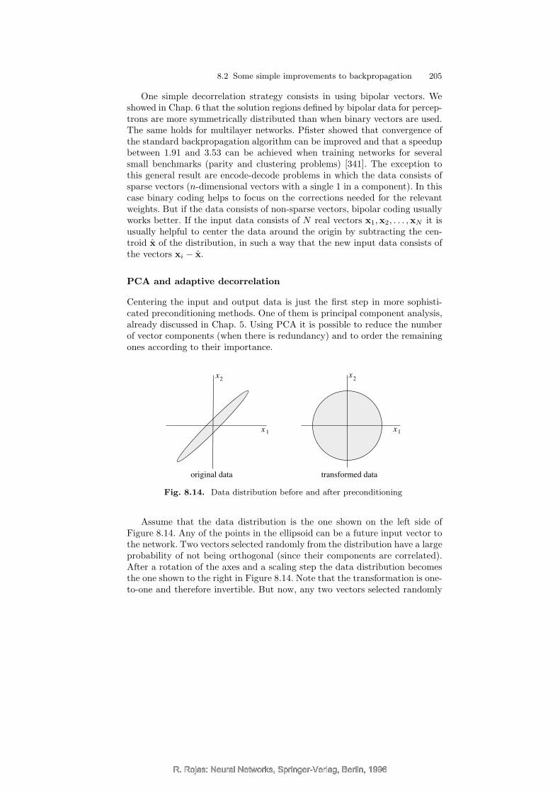
Centering the input and output data is just the first step in more sophisti-cated preconditioning methods. One of them is principal component analysis,already discussed in Chap. 5. Using PCA it is possible to reduce the numberof vector components (when there is redundancy) and to order the remainingones according to their importance.

x

x

transformed data

1

2x

2

x1

original data

Fig. 8.14. Data distribution before and after preconditioning

Assume that the data distribution is the one shown on the left side ofFigure 8.14. Any of the points in the ellipsoid can be a future input vector tothe network. Two vectors selected randomly from the distribution have a largeprobability of not being orthogonal (since their components are correlated).After a rotation of the axes and a scaling step the data distribution becomesthe one shown to the right in Figure 8.14. Note that the transformation is one-to-one and therefore invertible. But now, any two vectors selected randomly




from the new distribution (a sphere in n-dimensional space) have a greaterprobability of being orthogonal. The transformation of the data is linear (arotation followed by scaling) and can be applied to new data as it is provided.

Note that we do not know the exact form of the data distribution. All wehave is a training set (the dots in Figure 8.14) from which we can computethe optimal transformation. Principal component analysis is performed on theavailable data. This gives us a new encoding for the data set and also a lineartransformation for new data. The scaling factors are the reciprocal of thevariances of each component (see Exercise 2). PCA preconditioning speedsup backpropagation in most cases, except when the data consists of sparsevectors.

Silva and Almeida have proposed another data decorrelation technique,called Adaptive Data Decorrelation, which they use to precondition data [404].A linear layer is used to transform the input vectors, and another to trans-form the outputs of the hidden units. The linear layer consists of as manyoutput as input units, that is, it only applies a linear transformation to thevectors. Consider an n-dimensional input vector x = (x1, x2, . . . , xn). Denotethe output of the linear layer by (y1, y2, . . . , yn). The objective is to make theexpected value of the correlation coefficient rij of the i-th and j-th outputunits equal to Kronecker’s delta δij , i.e.,

rij =< yiyj >= δij .

The expected value is computed over all vectors in the data set. The algorithmproposed by Silva and Almeida is very simple: it consists in pulling the weightvector of the i-th unit away from the weight vector of the j-th unit, wheneverrij > 0 and in the direction of wj when rij < 0. The precise formula is

wk+1i = wk

i − βn∑

j 6=i

rijwkj ,

where wpm denotes the weight vector of the m-th unit at the p-th iteration

and β is a constant. Data normalization is achieved by including a positive ornegative term according to whether rii is smaller or greater than 1:

wk+1i = (1 + β)wk

i − βn∑

j=1

rijwkj .

The proof that the algorithm converges (under certain assumptions) canbe found in [404]. Adaptive Decorrelation can accelerate the convergence ofbackpropagation almost as well as principal component analysis, but is some-what sensitive to the choice of the constant β and the data selection process[341].



8.3 Adaptive step algorithms 207

Active data selection

For large training sets, redundancy in the data can make prohibitive the useof off-line backpropagation techniques. On-line backpropagation can still per-form well under these conditions if the training pairs are selected randomly.Since some of the fastest variations of backpropagation work off-line, there isa strong motivation to explore methods of reducing the size of the effectivetraining set.

Some authors have proposed training a network with a subset of the train-ing set, adding iteratively the rest of the training pairs [261]. This can bedone by testing the untrained pairs. If the error exceeds a certain threshold(for example if it is one standard deviation larger than the average error onthe effective training set), the pair is added to the effective training set andthe network is retrained when more than a certain number of pairs have beenrecruited [369].

8.3 Adaptive step algorithms

The class of adaptive step algorithms uses a very similar basic strategy: thestep size is increased whenever the algorithm proceeds down the error functionover several iterations. The step size is decreased when the algorithm jumpsover a valley of the error function. The algorithms differ according to the kindof information used to modify the step size.

In learning algorithms with a global learning rate, this is used to update allweights in the network. The learning rate is made bigger or smaller accordingto the iterations made so far.

P1

P2

P3

Fig. 8.15. Optimization of the error function with updates in the directions of theaxes

In algorithms with a local learning constant a different constant is used foreach weight. Whereas in standard backpropagation a single constant γ is used




to compute the weight corrections, in four of the algorithms considered beloweach weight wi has an associated learning constant γi so that the updates aregiven by

∆wi = −γi∂E

∂wi.

The motivation behind the use of different learning constants for each weightis to try to “correct” the direction of the negative gradient to make it pointdirectly to the minimum of the error function. In the case of a degenerate errorfunction, the gradient direction can lead to many oscillations. An adequatescaling of the gradient components can help to reach the minimum in fewersteps.

Figure 8.15 shows how the optimization of the error function proceedswhen only one-dimensional optimization steps are used (from point P1 toP2, and then to P3). If the lengths of the principal axes of the quadraticapproximation are very different, the algorithm can be slowed by an arbitraryfactor.

8.3.1 Silva and Almeida’s algorithm

The method proposed by Silva and Almeida works with different learningrates for each weight in a network [403]. Assume that the network con-sists of n weights w1, w2, . . . , wn and denote the individual learning rates byγ1, γ2, . . . , γn. We can better understand how the algorithm works by look-ing at Figure 8.16. The left side of the figure shows the level curves of aquadratic approximation to the error function. Starting the iteration processas described before and as illustrated with Figure 8.15, we can see that the al-gorithm performs several optimization steps in the horizontal direction. Sincehorizontal cuts to a quadratic function are quadratic, what we are trying tominimize at each step is one of the several parabolas shown on the right sideof Figure 8.16. A quadratic function of n variable weights has the general form

c21w21 + c22w

22 + · · ·+ c2nw

2n +

∑

i6=j

dijwiwj + C,

where c1, . . . , cn, the dij and C are constants. If the i-th direction is chosenfor a one-dimensional minimization step the function to be minimized has theform

c2iw2i + k1wi + k2,

where k1 and k2 are constants which depend on the values of the ‘frozen’variables at the current iteration point. This equation defines a family ofparabolas. Since the curvature of each parabola is given by c2i , they differjust by a translation in the plane, as shown in Figure 8.16. Consequently, itmakes sense to try to find the optimal learning rate for this direction, which isequal to 1/2c2i , as discussed in Sect. 8.1.1. If we have a different learning rate,optimization proceeds as shown on the left of Figure 8.16: the first parabola




is considered and the negative gradient direction is followed. The iterationsteps in the other dimensions change the family of parabolas which we haveto consider in the next step, but in this case the negative gradient directionis also followed. The family of parabolas changes again and so on. With thisquadratic approximation in mind the question then becomes, what are theoptimal values for γ1 to γn? We arrive at an additional optimization problem!

one-dimensional cuts

successive one-dimensionaloptimizations

Fig. 8.16. One-dimensional cuts: family of parabolas

The heuristic proposed by Almeida is very simple: accelerate if, in twosuccessive iterations, the sign of the partial derivative has not changed, anddecelerate if the sign changes. Let ∇iE

(k) denote the partial derivative ofthe error function with respect to weight wi at the k-th iteration. The initial

learning rates γ(0)i for i = 1, . . . , n are initialized to a small positive value.

At the k-th iteration the value of the learning constant for the next step isrecomputed for each weight according to

γ(k+1)i =

{

γ(k)i u if ∇iE

(k) · ∇iE(k−1) ≥ 0

γ(k)i d if ∇iE

(k) · ∇iE(k−1) < 0

The constants u (up) and d (down) are set by hand with u > 1 and d < 1.The weight updates are made according to

∆(k)wi = −γ(k)i ∇iE

(k) .

Note that due to the constants u and d the learning rates grow and decreaseexponentially. This can become a problem if too many acceleration steps areperformed successively. Obviously this algorithm does not follow the gradientdirection exactly. If the level curves of the quadratic approximation of the errorfunction are perfect circles, successive one-dimensional optimizations lead tothe minimum after n steps. If the quadratic approximation has semi-axes of




very different lengths, the iteration process can be arbitrarily slowed. To avoidthis, the updates can include a momentum term with rate α. Nevertheless,both kinds of corrections together are somewhat contradictory: the individuallearning rates can only be optimized if the optimization updates are strictlyone-dimensional. Tuning the constant α can therefore become quite problem-specific. The alternative is to preprocess the original data to achieve a moreregular error function. This can have a dramatic effect on the convergencespeed of algorithms which perform one-dimensional optimization steps.

8.3.2 Delta-bar-delta

The algorithm proposed by Jacobs is similar to Silva and Almeida’s, the maindifference being that acceleration of the learning rates is made with morecaution than deceleration. The algorithm is started with individual learningrates γ1, . . . , γn all set to a small value, and at the k-th iteration the newlearning rates are set to

γ(k+1)i =

γ(k)i + u if ∇iE

(k) · δ(k−1)i > 0

γ(k)i d if ∇iE

(k) · δ(k−1)i < 0

γ(k)i otherwise,

where u and d are constants and δ(k)i is an exponentially averaged partial

derivative in the direction of weight wi:

δ(k)i = (1 − φ)∇iE

(k) + φδ(k−1)i .

The constant φ determines what weight is given to the last averaged term.The weight updates are performed without a momentum term:

∆(k)wi = −γ(k)i ∇iE

(k).

The motivation for using an averaged gradient is to avoid excessive oscillationsof the basic algorithm. The problem with this approach, however, is thata new constant has to be set again by the user and its value can also behighly problem-dependent. If the error function has regions which allow agood quadratic approximation, then φ = 0 is optimal and we are essentiallyback to Silva and Almeida’s algorithm.

8.3.3 Rprop

A variant of Silva and Almeida’s algorithm is Rprop, first proposed by Ried-miller and Braun [366]. The main idea of the algorithm is to update the net-work weights using just the learning rate and the sign of the partial derivativeof the error function with respect to each weight. This accelerates learningmainly in flat regions of the error function as well as when the iteration has




arrived close to a local minimum. To avoid accelerating or decelerating toomuch, a minimum value for the learning rates γmin and a maximum value γmax

is enforced. The algorithm covers all of weight space with an n-dimensionalgrid of side γmin and an n-dimensional grid of side length γmax. The individ-ual one-dimensional optimization steps can move on all possible intermediategrids. The learning rates are updated in the k-th iteration according to

γ(k+1)i =

min(γ(k)i u, γmax) if ∇iE

(k) · ∇iE(k−1) > 0

max(γ(k)i d, γmin) if ∇iE

(k) · ∇iE(k−1) < 0

γ(k)i otherwise,

where the constants u and d satisfy u > 1 and d < 1, as usual. When ∇iE(k) ·

∇iE(k−1) ≥ 0 the weight updates are given by

∆(k)wi = −γ(k)i sgn(∇iE

(k)),

otherwise ∆(k)wi and ∇iE(k) are set to zero. In the above equation sgn(·)

denotes the sign function with the peculiarity that sgn(0) = 0.

cut of the error functionin one direction

Rprop approximation of theerror function

Fig. 8.17. Local approximation of Rprop

Figure 8.17 shows the kind of one-dimensional approximation of the errorfunction used by Rprop. It may seem a very imprecise approach, but it worksvery well in the flat regions of the error function. Schiffmann, Joost, andWerner tested several algorithms using a medical data set and Rprop producedthe best results, being surpassed only by the constructive algorithm calledcascade correlation [391] (see Chap. 14).

Table 8.1 shows the results obtained by Pfister on some of the CarnegieMellon Benchmarks [341]. The training was done on a CNAPS neurocom-puter. Backpropagation was coded using some optimizations (bipolar vectors,offset term, etc.). The table shows that BP did well for most benchmarks butfailed to converge in two of them. Rprop converged almost always (98% of




Table 8.1. Comparison of Rprop and batch backpropagation

benchmark generations time

BPRprop BP Rprop

sonar signals 109.7 82.0 8.6 s 6.9 s

vowels –1532.9 –593.6 s

vowels (decorrelated) 331.4 319.1 127.8 s123.6 s

NETtalk (200 words) 268.9 108.7 961.5 s389.6 s

protein structure 347.5 139.2 670.1 s269.1 s

digits – 159.5 –344.7 s

the time) and was faster by up to a factor of about 2.5 with respect to batchbackpropagation.

It should be pointed out that the vowels recognition task was presentedin two versions, one without and one with decorrelated inputs. In the lattercase, backpropagation did converge and was almost as efficient as Rprop. Thisshows how important the preprocessing of the input data can be. Note thatthe overall speedup obtained is limited because the version of backpropagationused for the comparison was rather efficient.

8.3.4 The Dynamic Adaption algorithm

We close our discussion of adaptive step methods with an algorithm basedon a global learning rate [386]. The idea of the method is to use the negativegradient direction to generate two new points instead of one. The point withthe lowest error is used for the next iteration. If it is the farthest away thealgorithm accelerates, by making the learning constant bigger. If it is thenearest one, the learning constant γ is reduced.

The k-th iteration of the algorithm consists of the following three steps:

• Compute

w(k1) = w(k) −∇E(w(k))γ(k−1) · ξw(k2) = w(k) −∇E(w(k))γ(k−1)/ξ

where ξ is a small constant (for example ξ = 1.7).• Update the learning rate:

γ(k) =

{γ(k−1) · ξ if E(w(k1)) ≤ E(w(k2))

γ(k−1)/ξ otherwise.

• Update the weights:

w(k+1) =

{w(k1) if E(w(k1)) ≤ E(w(k2))

w(k2) otherwise.



8.4 Second-order algorithms 213

The algorithm is not as good as the adaptive step methods with a locallearning constant, but is very easy to implement. The overhead involved is anextra feed-forward step.

8.4 Second-order algorithms

The family of second-order algorithms considers more information about theshape of the error function than the mere value of the gradient. A better iter-ation can be performed if the curvature of the error function is also consideredat each step. In second-order methods a quadratic approximation of the errorfunction is used [43]. Denote all weights of a network by the vector w. Denotethe error function by E(w). The truncated Taylor series which approximatesthe error function E is given by

E(w + h) ≈ E(w) +∇E(w)Th +1

2hT∇2E(w)h, (8.6)

where ∇2E(w) is the n×n Hessian matrix of second-order partial derivatives:

∇2E(w) =

∂2E(w)∂w2

1

∂2E(w)∂w1∂w2

· · · ∂2E(w)

∂w1∂wn

∂2E(w)∂w2∂w1

∂2E(w)∂w2

2· · · ∂

2E(w)∂w2∂wn

.... . .

...

∂2E(w)∂wn∂w1

∂2E(w)∂wn∂w2

· · · ∂2E(w)∂w2

n

.

The gradient of the error function can be computed by differentiating (8.6):

∇E(w + h)T ≈ ∇E(w)T + hT∇2E(w).

Equating to zero (since we are looking for the minimum of E) and solving, weget

h = −(∇2E(w))−1∇E(w), (8.7)

that is, the minimization problem can be solved in a single step if we havepreviously computed the Hessian matrix and the gradient, of course under theassumption of a quadratic error function.

Newton’s method works by using equation (8.7) iteratively. If we denotenow the weight vector at the k-th iteration by w(k), the new weight vectorw(k+1) is given by

w(k+1) = w(k) − (∇2E(w))−1∇E(w). (8.8)

Under the quadratic approximation, this will be a position where the gradienthas reduced its magnitude. Iterating several times we can get to the minimumof the error function.




However, computing the Hessian can become quite a difficult task. More-over, what is needed is the inverse of the Hessian. In neural networks wehave to repeat this computation on each new iteration. Consequently, manytechniques have been proposed to approximate the second-order informationcontained in the Hessian using certain heuristics.

Pseudo-Newton methods are variants of Newton’s method that work witha simplified form of the Hessian matrix [48]. The non-diagonal elements are allset to zero and only the diagonal elements are computed, that is, the secondderivatives of the form ∂2E(w)/∂w2

i . In that case equation (8.8) simplifies(for each component of the weight vector) to

w(k+1)i = w

(k)i − ∇iE(w)

∂2E(w)/∂w2i

. (8.9)

No matrix inversion is necessary and the computational effort involved infinding the required second partial derivatives is limited. In Sect. 8.4.3 weshow how to perform this computation efficiently.

Pseudo-Newton methods work well when the error function has a nicequadratic form, otherwise care should be exercised with the corrections, sincea small second-order partial derivative can lead to extremely large corrections.

8.4.1 Quickprop

In this section we consider an algorithm which tries to take second-orderinformation into account but follows a rather simple approach: only one-dimensional minimization steps are taken and information about the curvatureof the error function in the update directions is obtained from the current andthe last partial derivative of the error function in this direction.

cut of the error functionin one direction

Quickprop approximation of theerror function

Fig. 8.18. Local approximation of Quickprop

Quickprop is based on independent optimization steps for each weight. Aquadratic one-dimensional approximation of the error function is used. The




update term for each weight at the k-th step is given by

∆(k)wi = ∆(k−1)wi

( ∇iE(k)

∇iE(k−1) −∇iE(k)

)

, (8.10)

where it is assumed that the error function has been computed at steps (k−1)and k using the weight difference ∆(k−1)wi, obtained from a previous Quick-prop or an standard gradient descent step.

Note that if we rewrite (8.10) as

∆(k)wi = − ∇iE(k−1)

(∇iE(k) −∇iE(k))/∆(k−1)wi(8.11)

then the weight update in (8.11) is of the same form as the weight update in(8.9). The denominator is just a discrete approximation to the second-orderderivative ∂2E(w)/∂w2

i . Quickprop is therefore a discrete pseudo-Newtonmethod that uses so-called secant steps.

According to the value of the derivatives, Quickprop updates may becomevery large. This is avoided by limiting ∆(k)wi to a constant times ∆(k−1). See[130] for more details on the algorithm and the handling of different prob-lematic situations. Since the assumptions on which Quickprop is based aremore far-fetched than the assumptions used by, for example, Rprop, it is notsurprising that Quickprop has some convergence problems with certain tasksand requires careful handling of the weight updates [341].

8.4.2 QRprop

Pfister and Rojas proposed an algorithm that adaptively switches between theManhattan method used by Rprop and local one-dimensional secant steps likethose used by Quickprop [340, 341]. Since the resulting algorithm is a hybridof Rprop and Quickprop it was called QRprop.

QRprop uses the individual learning rate strategy of Rprop if two consecu-tive error function gradient components ∇iE

(k) and ∇iE(k−1) have the same

sign or one of these components equals zero. This produces a fast approach toa region of minimum error. If the sign of the gradient changes, we know thatwe have overshot a local minimum in this specific weight direction, so now asecond-order step (a Quickprop step) is taken. If we assume that in this direc-tion the error function is independent from all the other weights, a step basedon a quadratic approximation will be far more accurate than just steppinghalf way back as it is (indirectly) done by Rprop. Since the error functiondepends on all weights and since the quadratic approximation will be betterthe closer the two investigated points lie together, QRprop constrains the sizeof the secant step to avoid large oscillations of the weights. In summary:

i) As long as∇iE(k)·∇iE

(k−1) > 0 holds, Rprop steps are performed becausewe assume that a local minimum lies ahead.




ii) If ∇iE(k) · ∇iE

(k−1) < 0, which suggests that a local minimum has beenovershot, then, unlike Rprop, neither the individual learning rate γi northe weight wi are changed. A “marker” is defined by setting ∇iE

(k) := 0and the secant step is performed in the subsequent iteration.

iii) If ∇iE(k) · ∇iE

(k−1) = 0, this means that either a marker was set inthe previous step, or one of the gradient components is zero because alocal minimum has been directly hit. In both cases we are near a localminimum and the algorithm performs a second-order step. The secantapproximation is done using the gradient information provided by ∇iE

(k)

and∇iE(k−2). The second-order approximation is used even when∇iE

(k) ·∇iE

(k−2) > 0. Since we know that we are near a local minimum (and verylikely we have already overshot it in the previous step), the second-orderapproximation is still a better choice than just stepping halfway back.

iv) In the secant step the quadratic approximation

qi := |∇iE(k))/(∇iE

(k) −∇iE(k−2))|

is constrained to a certain interval to avoid very large or very small up-dates.

Therefore, the k-th iteration of the algorithm consists of the following steps:

Step 1: Update the individual learning rates

if (∇iE(k) · ∇iE

(k−1) = 0) thenif (∇iE

(k) 6= (∇iE(k−2)) then

qi = max(

d,min(

1/u,∣∣∣

∇iE(k)

∇iE(k)−∇iE(k−2)

∣∣∣

))

elseqi = 1/u

endifendif

γ(k)i =

min(u · γ(k−1)i , γmax) ∇iE

(k) · ∇iE(k−1) > 0

γ(k−1)i if ∇iE

(k) · ∇iE(k−1) < 0

max(qi · γ(k−1)i , γmin) ∇iE

(k) · ∇iE(k−1) = 0

Step 2: Update the weights

w(k+1)i =

w(k)i − γ(k)

i · sgn(∇iE(k)) if ∇iE

(k) · ∇iE(k−1) ≥ 0

w(k)i otherwise

If (∇iE(k) · ∇iE

(k−1) < 0) set ∇iE(k) := 0.




The constants d, u, γmin, and γmax must be chosen in advance as for otheradaptive steps methods. QRprop has shown to be an efficient algorithm thatcan outperform both of its original algorithmic components. Table 8.2 showsthe speedup obtained with QRprop relative to Rprop for the Carnegie Mellonbenchmarks [341].

Table 8.2. Speedup of QRprop relative to Rprop

benchmark speedup

sonar signals 1.01

vowels 1.33

vowels (decorrelated) 1.30

NETtalk (200 words) 1.02

protein structure 1.14

digits 1.29

average 1.18

8.4.3 Second-order backpropagation

In this section we introduce second-order backpropagation, a method to effi-ciently compute the Hessian of a linear network of one-dimensional functions.This technique can be used to get explicit symbolic expressions or numericalapproximations of the Hessian and could be used in parallel computers toimprove second-order learning algorithms for neural networks. Methods forthe determination of the Hessian matrix in the case of multilayered networkshave been studied recently [58].

We show how to efficiently compute the elements of the Hessian matrixusing a graphical approach, which reduces the whole problem to a computationby inspection. Our method is more general than the one developed in [58]because arbitrary topologies can be handled. The only restriction we imposeon the network is that it should contain no cycles, i.e., it should be of thefeed-forward type. The method is of interest when we do not want to deriveanalytically the Hessian matrix each time the network topology changes.

Second-order derivatives

We investigate the case of second-order derivatives, that is, expressions of theform ∂2F/∂wi∂wj , where F is the network function as before and wi and wj

are network’s weights. We can think of each weight as a small potentiometerand we want to find out what happens to the network function when theresistance of both potentiometers is varied.




F(x)

x

s =

node qF (x)

1l q

F (x)2l q

F (x)ml q

F (x)ml qF (x)

1l q

g(s)

+ ... +

network

Fig. 8.19. Second-order computation

Figure 8.19 shows the general case. Let us assume, without loss of general-ity, that the input to the network is the one-dimensional value x. The networkfunction F is computed at the output node with label q (shown shaded) forthe given input value. We can also think of the inputs to the output nodeas network functions computed by subnetworks of the original network. Letus call these functions F`1q, F`2q, . . . , F`mq. If the one-dimensional function atthe output node is g, the network function is the composition

F (x) = g(F`1q(x) + F`2q(x) + . . .+ F`mq(x)).

We are interested in computing ∂2F (x)/∂wi∂wj for two given network weightswi and wj . Simple differential calculus tells us that

∂2F (x)

∂wi∂wj= g′′(s)

∂s

∂wi

∂s

∂wj

+ g′(s)

(∂2F`1q(x)

∂wi∂wj+ · · ·+ ∂2F`mq(x)

∂wi∂wj

)

,

where s = F`1q(x) + F`2q(x) + . . . + F`mq(x). This means that the desiredsecond-order partial derivative consists of two terms: the first is the secondderivative of g evaluated at its input multiplied by the partial derivatives of thesum of them subnetwork functions F`1q, . . . , F`mq, once with respect to wi andonce with respect to wj . The second term is the first derivative of g multipliedby the sum of the second-order partial derivatives of each subnetwork functionwith respect to wi and wj . We call this term the second-order correction. Therecursive structure of the problem is immediately obvious. We already have analgorithm to compute the first partial derivatives of any network function with




respect to a weight. We just need to use the above expression in a recursivemanner to obtain the second-order derivatives we want.

We thus extend the feed-forward labeling phase of the backpropagationalgorithm in the following manner: at each node which computes a one-dimensional function f we will store three values: f(x), f ′(x) and f ′′(x), wherex represents the input to this node. When looking for the second-order deriva-tives we apply the recursive strategy given above. Figure 8.20 shows the mainidea:

wi

wj

backpropagation path

for

backpropagation path

for

wi

wj

Fig. 8.20. Intersecting paths to a node

• Perform the feed-forward labeling step in the usual manner, but storeadditionally at each node the second derivative of the node’s functionevaluated at its input

• Select two weights wi and wj and an output node whose associated networkfunction we want to derive. The second-order partial derivative of thenetwork function with respect to these weights is the product of the storedg′′ value with the backpropagation path value from the output node up toweight wi and with the backpropagation path value from the output nodeup to weight wj . If the backpropagation paths for wi and wj intersect,a second-order correction is needed which is equal to the stored value ofg′ multiplied by the sum of the second-order derivative with respect towi and wj of all subnetwork function inputs to the node which belong tointersecting paths.

This looks like an intricate rule, but it is again the chain rule for second-order derivatives expressed in a recursive manner. Consider the multilayerperceptron shown in Figure 8.21. A weight wih in the first layer of weightsand a weight wjm in the second layer can only interact at the output nodem. The second derivative of Fm with respect to wih and wjm is just thestored value f ′′ multiplied by the stored output of the hidden unit j and thebackpropagation path up to wih, that is, whmh

′xi. Since the backpropagationpaths for wih and wjm do not intersect, this is the required expression. Thisis also the expression found analytically by Bishop [1993].




w

w

ih

jm

Backpropagation path

for w

Backpropagation path

for w

ih

jm

ff '

f ''

xi

hh'

h''

input

layer

hidden

layer

Fm

whm

Fig. 8.21. Multilayer perceptron

In the case where one weight lies in the backpropagation path of another,a simple adjustment has to be made. Let us assume that weight wik lies inthe backpropagation path of weight wj . The second-order backpropagationalgorithm is performed as usual and the backward computation proceeds upto the point where weight wik transports an input to a node k for whicha second-order correction is needed. Figure 8.22 shows the situation. Theinformation transported through the edge with weight wik is the subnetworkfunction Fik. The second-order correction for the node with primitive functiong is

g′∂2Fik

∂wik∂wj= g′

∂2wikFi

∂wik∂wj,

but this is simply

g′∂Fi

∂wj,

since the subnetwork function Fi does not depend on wik. Thus, the second-order backpropagation method must be complemented by the following rule:

• If the second-order correction to a node k with activation function g in-volves a weight wik (that is, a weight directly affecting node k) and a nodewj , the second-order correction is just g′ multiplied by the backpropaga-tion path value of the subnetwork function Fi with respect to wj .

Explicit calculation of the Hessian

For the benefit of the reader, we put together all the pieces of what we callsecond-order backpropagation in this section. We consider the case of a singleinput pattern into the network, since the more general case is easy to handle.




f gwikf '

f ''

g'

g''F

jw

x

x

x

1

2

n

Fi

Fig. 8.22. The special case

Algorithm 8.4.1 Second-order backpropagation

i) Extend the neural network by adding nodes which compute the squareddifference of each component of the output and the expected target val-ues. Collect all these differences at a single node whose output is theerror function of the network. The activation function of this node is theidentity.

ii) Label all nodes in the feed-forward phase with the result of computingf(x), f ′(x), and f ′′(x), where x represents the global input to each nodeand f its associated activation function.

iii) Starting from the error function node in the extended network, computethe second-order derivative of E with respect to two weights wi and wj ,by proceeding recursively in the following way:

iii.1) The second-order derivative of the output of a node G with activa-tion function g with respect to two weights wi and wj is the productof the stored g′′ value with the backpropagation path values betweenwi and the node G and between wj and the node G. A second-ordercorrection is needed if both backpropagation paths intersect.

iii.2) The second-order correction is equal to the product of the stored g′

value with the sum of the second-order derivative (with respect towi and wj) of each node whose output goes directly to G and whichbelongs to the intersection of the backpropagation paths of wi andwj .

iii.3) In the special case that one of the weights, for example, wi, connectsnode h directly to node G, the second-order correction is just g′

multiplied by the backpropagation path value of the subnetworkfunction Fh with respect to wj .




Example of second-order backpropagation

Consider the network shown in Figure 8.23, commonly used to compute theXOR function. The left node is labeled 1, the right node 2. The input values xand y are kept fixed and we are interested in the second-order partial derivativeof the network function F2(x, y) with respect to the weights w1 and w2.

x

y

f g

w1

w2

w3

w 5

w4

f '

f ''

g'

g''F

2

F1

node 1 node 2

Fig. 8.23. A two unit network

By mere inspection and using the recursive method mentioned above, wesee that the first term of ∂2F2/∂w1∂w2 is the expression

g′′(w3x+ w5y + w4f(w1x+ w2y))(w4f′(w1x+ w2y)x)(w4f

′(w1x+ w2y)y).

In this expression (w4f′(w1x+w2y)x) is the backpropagation path value from

the output of the node which computes the function f , including multiplica-tion by the weight w4 (that is the subnetwork function w4F1), up to the weightw1. The term (w4f

′(w1x+w2y)y) is the result of backpropagation for w4F1 upto w2. The second-order correction needed for computation of ∂2F2/∂w1∂w2

is

g′(w3x+ w5y + w4f(w1x+ w2y))∂2w4F1

∂w1∂w2.

Since it is obvious that

∂2w4F1

∂w1∂w2= w4

∂2F1

∂w1∂w2= w4f

′′(w1x+ w2y)xy

we finally get

∂2F2

∂w1∂w2= g′′(w3x+ w5y + w4f(w1x+ w2y))

× (w4f′(w1x+ w2y)x)(w4f

′(w1x+ w2y)y)

+ g′(w3x+ w5y + w4f(w1x+ w2y))w4f′′(w1x+ w2y)xy.

The reader can visually check the following expression:

∂2F2

∂w1∂w5= g′′(w3x+ w5y + w4f(w1x+ w2y))(w4f

′(w1x+ w2y)x)y.




In this case no second-order correction is needed, since the backpropagationpaths up to w1 and w5 do not intersect.

A final example is the calculation of the whole Hessian matrix for thenetwork shown above (Figure 8.23). We omit the error function expansion andcompute the Hessian of the network function F2 with respect to the network’sfive weights. The labelings of the nodes are f , f ′, and f ′′ computed over theinput w1x + w2y, and g, g′, g′′ computed over the input w4f(w1x + w2y) +w3x+w5y. Under these assumptions the components of the upper triangularpart of the Hessian are the following:

H11 = g′′w24f

′2x2 + g′w4f′′x2

H22 = g′′w24f

′2y2 + g′w4f′′y2

H33 = g′′x2

H44 = g′′f2

H55 = g′′y2

H12 = g′′w24f

′2xy + g′w4f′′xy

H13 = g′′w4f′x2

H14 = g′′w4f′xf + g′f ′x

H15 = g′′w4f′xy

H23 = g′′w4f′yx

H24 = g′′w4f′yf + g′f ′y

H25 = g′′w4f′y2

H34 = g′′xf

H35 = g′′xy

H45 = g′′yf

All these results were obtained by simple inspection of the network shownin Figure 8.23. Note that the method is totally general in the sense that eachnode can compute a different activation function.

Some conclusions

With some experience it is easy to compute the Hessian matrix even for con-voluted feed-forward topologies. This can be done either symbolically or nu-merically. The importance of this result is that once the recursive strategyhas been defined it is easy to implement in a computer. It is the same kind ofdifference as the one existing between the chain rule and the backpropagationalgorithm. The first one gives us the same result as the second, but backprop-agation tries to organize the data in such a way that redundant computationsare avoided. This can also be done for the method described here. Calculationof the Hessian matrix involves repeated computation of the same terms. In




this case the network itself provides us with a data structure in which we canstore partial results and with which we can organize the computation. Thisexplains why standard and second-order backpropagation are also of interestfor computer algebra systems. It is not very difficult to program the methoddescribed here in a way that minimizes the number of arithmetic operationsneeded. The key observation is that the backpropagation path values can bestored to be used repetitively and that the nodes in which the backpropaga-tion paths of different weights intersect need to be calculated only once. It isthen possible to optimize computation of the Hessian using graph traversingalgorithms.

A final observation is that computing the diagonal of the Hessian matrixinvolves only local communication in a neural network. Since the backprop-agation path to a weight intersects itself in its whole length, computation ofthe second partial derivative of the associated network function of an outputunit with respect to a given weight can be organized as a recursive backwardcomputation over this path. Pseudo-Newton methods [48] can profit from thiscomputational locality.

8.5 Relaxation methods

The class of relaxation methods includes all those techniques in which thenetwork weights are perturbed and the new network error is compared directlyto the previous one. Depending on their relative magnitudes a decision is takenregarding the subsequent iteration steps.

8.5.1 Weight and node perturbation

Weight perturbation is a learning strategy which has been proposed to avoidcalculating the gradient of the error function at each step. A discrete approx-imation to the gradient is made at each iteration by taking the initial weightvector w in weight space and the value E(w) of the error function for thiscombination of parameters. A small perturbation β is added to the weight wi.The error E(w′) at the new point w′ in weight space is computed and theweight wi is updated using the increment

∆wi = −γE(w′)− E(w)

β.

This step is repeated iteratively, randomly selecting the weight to be updated.The discrete approximation to the gradient is especially important for VLSIchips in which the learning algorithm is implemented with minimal hardwareadditional to that needed for the feed-forward phase [216].

Another alternative which can provide faster convergence is perturbing nota weight, but the output oi of the i-th node by ∆oi. The difference E −E′ in



8.5 Relaxation methods 225

the error function is computed and if it is positive, the new error E′ could beachieved with the output oi+∆oi for the i-th node. If the activation function isa sigmoid, the desired weighted input to node i is

∑mk=1 w

′kxk = s−1(oi+∆oi).

If the previous weighted input was∑m

k=1 wkxk, then the new weights are givenby

w′k = wk

s−1(oi +∆oi)∑m

k=1 wkxkfor k = 1, . . . ,m.

The weights are updated in proportion to their relative size. To avoid alwayskeeping the same proportions, a stochastic factor can be introduced or a nodeperturbation step can be alternated with a weight perturbation step.

8.5.2 Symmetric and asymmetric relaxation

According to the analysis we made in Sect. 7.3.3 of two layered networkstrained with backpropagation, the backpropagated error up to the outputlayer can be written as

δ(2) = D2e,

where e is the column vector whose components are the derivatives of thecorresponding components of the quadratic error, and D2 is a diagonal matrixas defined in Chap. 7. We can try to reduce the magnitude of the error e tozero by adjusting the matrix W2 in a single step. Since the desired targetvector is t, the necessary weighted input at the output nodes is s−1(t). Thismeans that we want the equation

o(1)W2 = s−1(t)

to hold for all the p possible input patterns. If we arrange all vectors o(1) asthe rows of a p × k matrix O1 and all targets as the rows of a p×m matrixT, we are looking for the matrix W2 for which

O1W2 = s−1(T) (8.12)

holds. In general this matrix equation may have no solution for W2, but wecan compute the matrix which minimizes the quadratic error for this equality.We show in Sects. 9.2.4 and ?? that if O+

1 is the so-called pseudoinverse ofO1, then W2 is given by

W2 = O+1 s

−1(T).

After computing W2 we can ask what is the matrix O1 which minimizes thequadratic deviation from equality in (8.12). We compute intermediate targetsfor the hidden units, which are given by the rows of the matrix

O′1 = s(−1)(T)W+

2 .

The new intermediate targets can now be used to obtain an update for thematrix W1 of weights between input sites and hidden units. The pseudoinversecan be computed with the method discussed in Sect. 9.2.4.




Note that this method is computationally intensive for every “pseudoin-verse” step. The weight corrections are certainly much more accurate than inother algorithms but these high-powered iterations demand many computa-tions for each of the two matrices. If the error function can be approximatednicely with a quadratic function, the algorithm converges very fast. If the inputdata is highly redundant, then the pseudoinverse step can be very inefficientwhen compared to on-line backpropagation, for example.

The algorithm described is an example of symmetric relaxation, since boththe targets T and the outputs of the hidden units are determined in a backand forth kind of approach.

8.5.3 A final thought on taxonomy

The contents of this chapter can be summarized using Figure 8.24. The fastvariations of backpropagation have been divided into two columns: gradientdescent and relaxation methods. Algorithms in the first column use informa-tion about the error function’s partial derivatives. Algorithms in the secondcolumn try to adjust the weights to fit the problem in a stochastic way orsolving a linear subproblem.

The three rows in Figure 8.24 show the kinds of derivative used. First-orderalgorithms work with the first partial derivatives, second-order algorithmswith the second partial derivatives. In between we have adaptive first-ordermethods that from first-order information extract an approximation to partsof the Hessian matrix.

Standard backpropagation is a first-order gradient descent method. How-ever, since on-line backpropagation does not exactly follow the gradient’s di-rection, it also partially qualifies as a relaxation method. The adaptive stepmethods (DBD, Rprop, etc.) are also a combination of gradient descent andrelaxation. Quickprop is an algorithm which approximates second-order infor-mation but which updates the weights separately using a kind of relaxationapproach.

The adaptive first-order methods can be also divided in two groups: inthe first a single global learning rate is used, in the second there is a learningrate for each weight. The conjugate gradient methods of numerical analysisrely also on a first-order approximation of second-order features of the errorfunction.

8.6 Historical and bibliographical remarks

This survey of fast learning algorithms is by no means complete. We havedisregarded constructive algorithms of the type reviewed in Chap. 14. Wehave only given a quick overview of some of the main ideas that have beendeveloped in the last decade. There is a large amount of literature on nonlinearoptimization that should be reviewed by anyone wishing to improve current



8.6 Historical and bibliographical remarks 227

gradient descent relaxation

first

order

second

order

adaptive

first

order

backpropagation

off-line

momentum

weight

perturbation

symmetric

relaxation

(pseudoinverse)Newton's method

Pseudo-Newton

global

adaptive

learning

constant

local

adaptive

learning

constant

CG

methods

asymmetric

relaxation

on-line

QuickPropQRprop

Almeida's

DBD

Rprop

Fig. 8.24. Taxonomy of learning algorithms

learning methods for multilayer networks. Classical CG algorithms and somevariants developed specially for neural networks are interesting in this respect[315].

A different approach has been followed by Karayiannis and Venetsanopou-los who use a type of what is called a continuation method [235]. The networkis trained to minimize a given measure of error, which is iteratively changedduring the computation. One can start solving a linear regression problem andintroduce the nonlinearities slowly. The method could possibly be combinedwith some of the other fast learning methods.

A factor which has traditionally hampered direct comparisons of learningalgorithms is the wide variety of benchmarks used. Only in a few cases havelarge learning problems taken from public domain databases been used. Someefforts to build a more comprehensive set of benchmarks have been announced.




Exercises

1. Prove that the value of the learning constant given by equation (8.5) infact produces exact learning of the j input pattern to a linear associator.Derive the expression for `2.

2. Show how to construct the linear transformation that maps an ellipsoidaldata distribution to a sphere. Assume that the training set consists of Npoints (Sect. 8.2.4).

3. Compare Rprop and Quickprop using a small benchmark (for example the8-bit parity problem).

4. Train a neural network using: a) Backpropagation and a piecewise linearapproximation of the sigmoid; b) A table of values of the sigmoid and itsderivative.


8 fast learning algorithms - freie universitätpage.mi.fu-berlin.de/rojas/neural/chapter/k8.pdf ·...

Documents