8. antennas and radiating systems · 8.1 introduction antennas radiation fundamentals antenna...
TRANSCRIPT

Dr. Rakhesh Singh Kshetrimayum
8. Antennas and Radiating Systems
Dr. Rakhesh Singh Kshetrimayum
4/26/20161 Electromagnetic Field Theory by R. S. Kshetrimayum
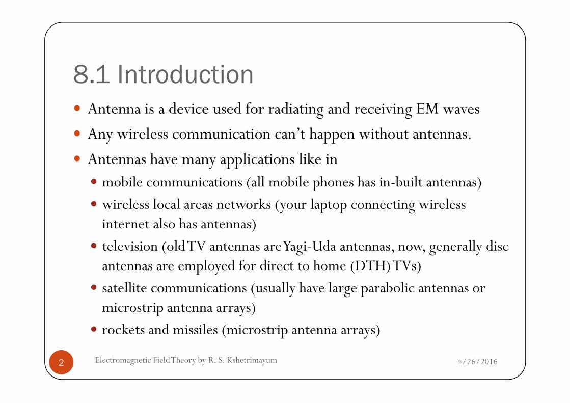
8.1 Introduction Antenna is a device used for radiating and receiving EM waves
Any wireless communication can’t happen without antennas.
Antennas have many applications like in mobile communications (all mobile phones has in-built antennas)
wireless local areas networks (your laptop connecting wireless
4/26/2016Electromagnetic Field Theory by R. S. Kshetrimayum2
wireless local areas networks (your laptop connecting wireless internet also has antennas)
television (old TV antennas are Yagi-Uda antennas, now, generally disc antennas are employed for direct to home (DTH) TVs)
satellite communications (usually have large parabolic antennas or microstrip antenna arrays)
rockets and missiles (microstrip antenna arrays)

8.1 Introduction
Antennas
Radiation fundamentals
Antenna pattern and parameters
Types of antennas
Antenna arrays
When does a charge radiate?
4/26/2016Electromagnetic Field Theory by R. S. Kshetrimayum3
Fig. 8.1 Antennas (cover antenna pattern and parameters after types of antennas)
charge radiate?
Wave equation for potential functions
Solution of wave equation for potential functions
Hertz dipole
Dipole antenna
Loop antenna

8.2 Radiation fundamentals8.2.1 When does a charge radiates? accelerating/decelerating charges radiate EM waves
r
4/26/2016Electromagnetic Field Theory by R. S. Kshetrimayum4
Fig. 8.2 A giant sphere of radius r with a source of EM wave at its origin
Source
r

8.2 Radiation fundamentals Consider a giant sphere of radius r which encloses the source
of EM waves at the origin (Fig. 8.2)
The total power passing out of the spherical surface is given by Poynting theorem,
4/26/2016Electromagnetic Field Theory by R. S. Kshetrimayum5
( ) ( )∫∫ •×=•= ∗sdHEsdSrP avgtotal
rrrrrRe
( )lim
totalP P r
r=
→∝

8.2 Radiation fundamentals This is the energy per unit time that is radiated into infinity
and it never comes back to the source
The signature of radiation is irreversible flow of energy away from the source
4/26/2016Electromagnetic Field Theory by R. S. Kshetrimayum6
from the source
Let us analyze the following three cases:
CASE 1: A stationary charge will not radiate. no flow of charge =>no current=>no magnetic field=>no
radiation

8.2 Radiation fundamentalsCASE 2: A charge moving with constant velocity will not radiate.
The area of the giant sphere of Fig. 8.2 is 4 r2
So for the radiation to occur Poynting vector must decrease no faster than 1/r2
from Coloumb’s law, electrostatic fields decrease as 1/r2,
4/26/2016Electromagnetic Field Theory by R. S. Kshetrimayum7
from Coloumb’s law, electrostatic fields decrease as 1/r ,
whereas Biot Savart’s law states that magnetic fields decrease as 1/r2
So the total decrease in the Poynting vector is proportional to 1/r4 no radiation
CASE 3: A time varying current or acceleration (or deceleration) of charge will radiate.

8.2 Radiation fundamentals Basic radiation equation:
where L=length of current element, m
=time changing current, As-1(units)
dt
dvQ
dt
diL =
di
4/26/2016Electromagnetic Field Theory by R. S. Kshetrimayum8
=time changing current, As-1(units)
Q=charge, C
=acceleration of charge, ms-2
dt
di
dt
dv
8.2 Radiation fundamentals
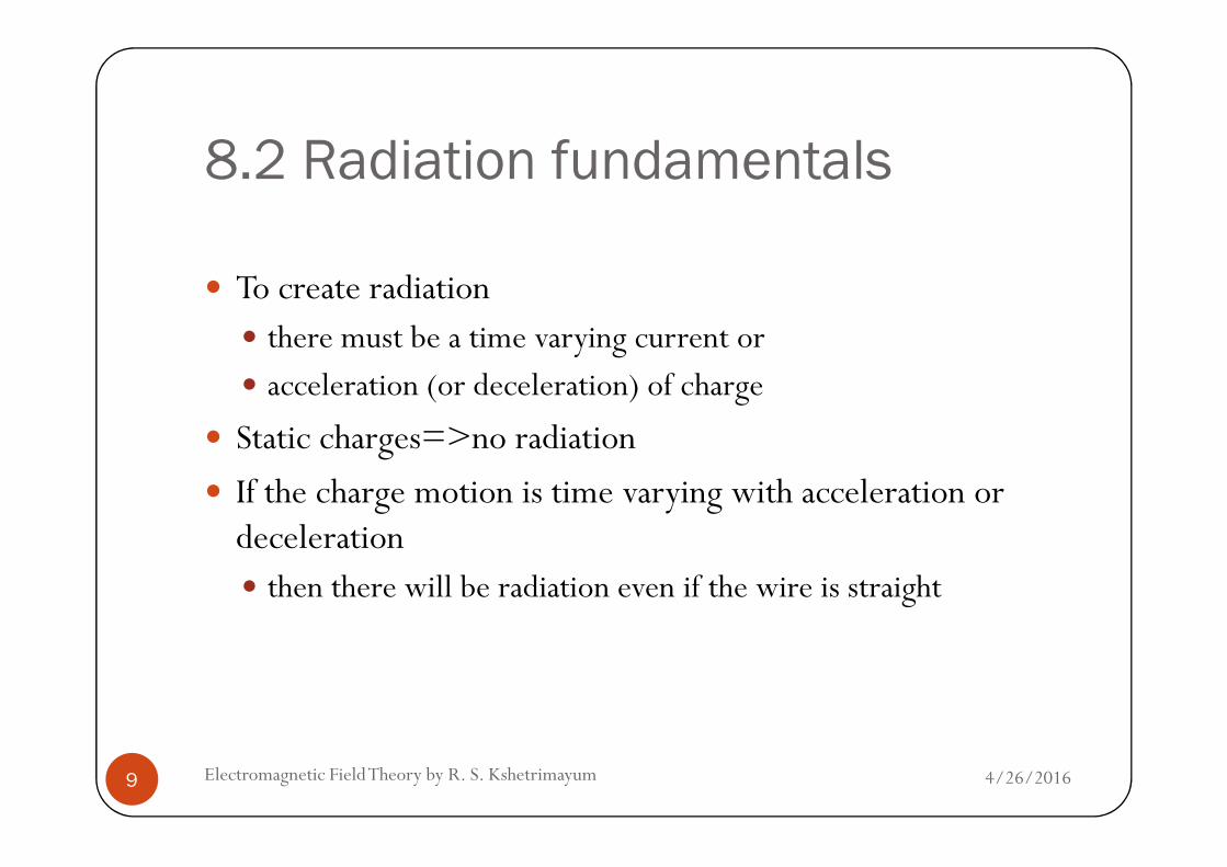
To create radiation there must be a time varying current or
acceleration (or deceleration) of charge
Static charges=>no radiation
4/26/2016Electromagnetic Field Theory by R. S. Kshetrimayum9
Static charges=>no radiation
If the charge motion is time varying with acceleration or deceleration then there will be radiation even if the wire is straight
8.2 Radiation fundamentals
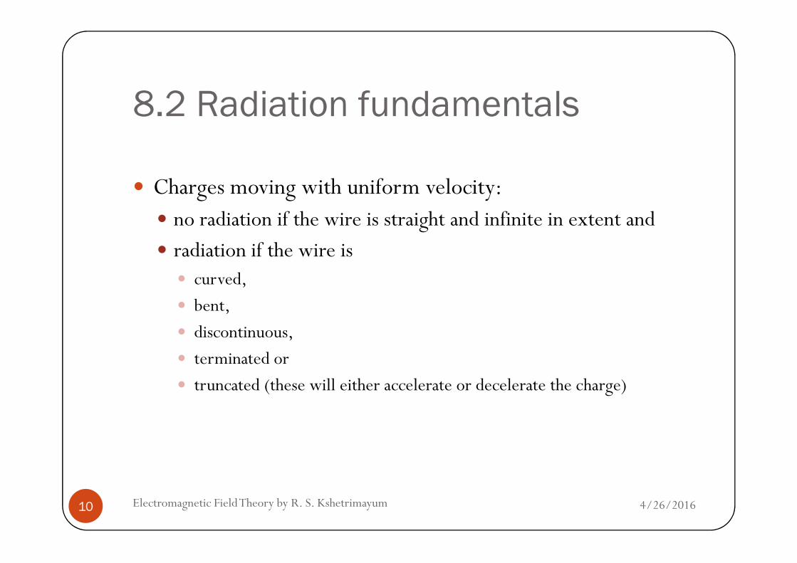
Charges moving with uniform velocity: no radiation if the wire is straight and infinite in extent and
radiation if the wire is curved,
4/26/2016Electromagnetic Field Theory by R. S. Kshetrimayum10
curved,
bent,
discontinuous,
terminated or
truncated (these will either accelerate or decelerate the charge)

8.2 Radiation fundamentals For radiation, electric field will have a transversal component
instead of radial component
whenever a charge accelerates or decelerates
Example 8.1
Prove that in order to have radiation the electric field must
4/26/2016Electromagnetic Field Theory by R. S. Kshetrimayum11
Prove that in order to have radiation the electric field must have spatial variation as 1/r where r is the distance from the source

8.2 Radiation fundamentals 8.2.2 Wave equation for potential functions
One of the Maxwell’s equation
Hence
Putting this in the following Maxwell’s equation
0=•∇ Br
ABrr
×∇=
B∂r
r ( )A×∇∂r
r
4/26/2016Electromagnetic Field Theory by R. S. Kshetrimayum12
t
BE
∂
∂−=×∇
rr ( )
t
AE
∂
×∇∂−=×∇
rr
0A
Et
∂⇒∇× + =
∂
rr A
E Vt
∂⇒ + = −∇
∂
rr

8.2 Radiation fundamentals Putting this in the following Maxwell’s equation
ε
ρ=•∇ E
r
ε
ρ−=
∇+
∂
∂•∇ V
t
Ar
2AV
t
ρ
ε
∂⇒∇ • + ∇ = −
∂
r
4/26/2016Electromagnetic Field Theory by R. S. Kshetrimayum13
Another Maxwell’s equation
Simplifies to
t ε∂
t
EJB
∂
∂+=×∇
rrr
µεµ
( )t
Vt
A
JAAA∂
∇+
∂
∂∂
−=∇−•∇∇=×∇×∇
r
rrrrµεµ2

8.2 Radiation fundamentals Lorentz Gauge condition
Applying above condition
0=∂
∂+•∇
t
VA µεr
∂ ∂ ∂r
r r
4/26/2016Electromagnetic Field Theory by R. S. Kshetrimayum14
22
2
V AA J V
t t tµε µ µε
∂ ∂ ∂ ⇒∇ − − ∇ = − + ∇
∂ ∂ ∂
rr r
22
2
AA J
tµε µ
∂⇒∇ − = −
∂
rr r
( )ε
ρ−=∇+
∂
•∇∂V
t
A 2
r 22
2
VV
t
ρµε
ε
∂⇒∇ − = −
∂
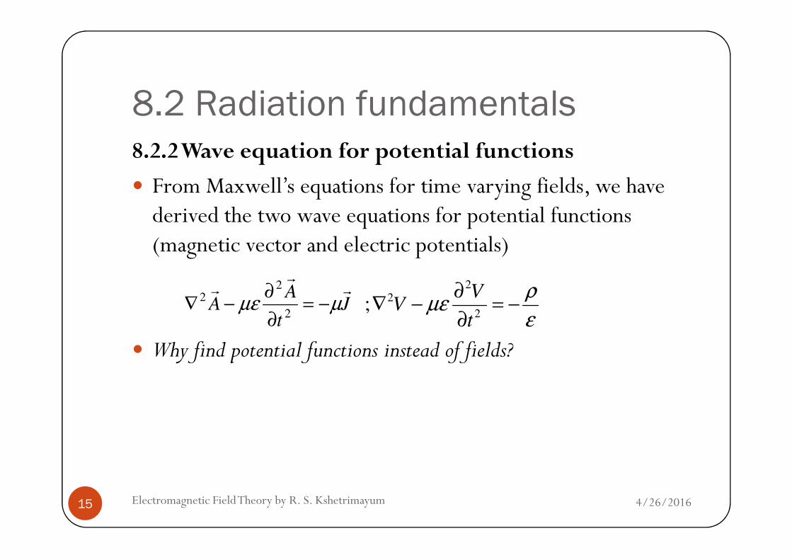
8.2 Radiation fundamentals8.2.2 Wave equation for potential functions
From Maxwell’s equations for time varying fields, we have derived the two wave equations for potential functions (magnetic vector and electric potentials)
rr
r ∂ 2 2V ρ∂
4/26/2016Electromagnetic Field Theory by R. S. Kshetrimayum15
Why find potential functions instead of fields?
Jt
AA
rr
rµµε −=
∂
∂−∇
2
22
22
2;
VV
t
ρµε
ε
∂∇ − = −
∂
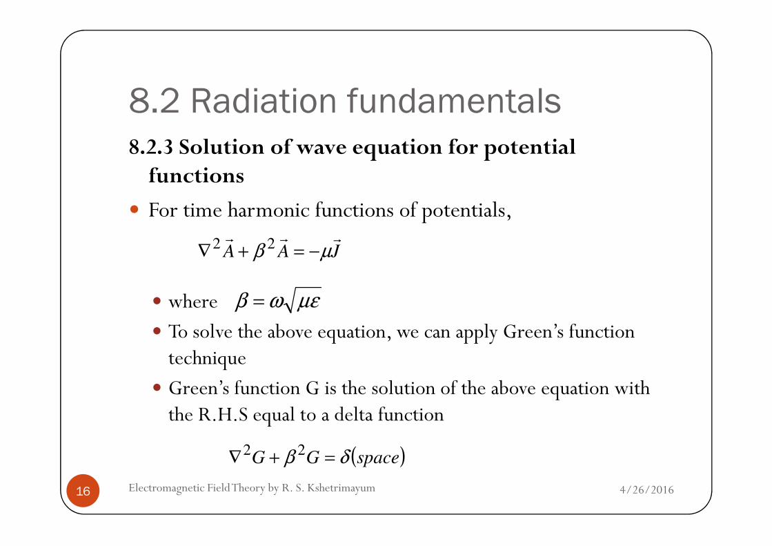
8.2 Radiation fundamentals8.2.3 Solution of wave equation for potential
functions
For time harmonic functions of potentials,
JAArrr
µβ −=+∇ 22
4/26/2016Electromagnetic Field Theory by R. S. Kshetrimayum16
where
To solve the above equation, we can apply Green’s function technique
Green’s function G is the solution of the above equation with the R.H.S equal to a delta function
( )spaceGG δβ =+∇ 22
µεωβ =
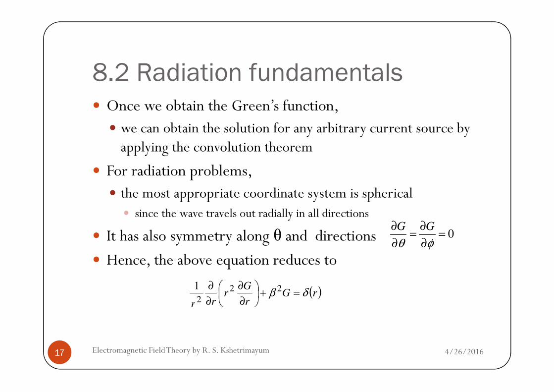
8.2 Radiation fundamentals Once we obtain the Green’s function,
we can obtain the solution for any arbitrary current source by applying the convolution theorem
For radiation problems, the most appropriate coordinate system is spherical
4/26/2016Electromagnetic Field Theory by R. S. Kshetrimayum17
the most appropriate coordinate system is spherical since the wave travels out radially in all directions
It has also symmetry along θ and directions
Hence, the above equation reduces to
0G G
θ φ
∂ ∂= =
∂ ∂
( )rGr
Gr
rrδβ =+
∂
∂
∂
∂ 22
2
1

8.2 Radiation fundamentals Putting Ψ= G r,
For r not equal to 0,
( )rrr
δβ =Ψ+Ψ∂
∂ 2
2
2
4/26/2016Electromagnetic Field Theory by R. S. Kshetrimayum18
Therefore,
02
2
2
=Ψ+Ψ∂
∂β
r
rjrjBeAe
ββ +− +=Ψ

8.2 Radiation fundamentals Since the radiation travels radially in positive r direction
negative r direction is not physically feasible for a source of a field, we get,
rjAe
β−=Ψ
rjβ−
4/26/2016Electromagnetic Field Theory by R. S. Kshetrimayum19
From example 8.2, we can find the constant A and hence
r
AeG
rjβ−
=
r
eGA
rj
ππ
β
4;
4
1 −
==
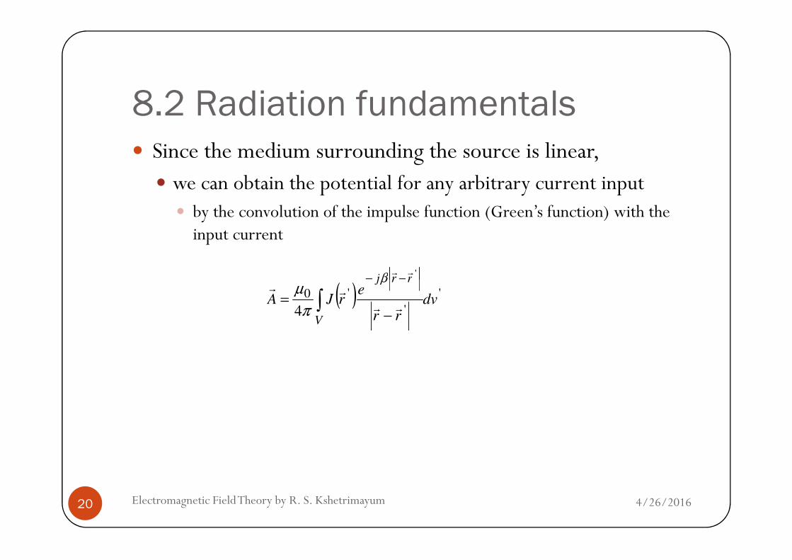
8.2 Radiation fundamentals Since the medium surrounding the source is linear,
we can obtain the potential for any arbitrary current input by the convolution of the impulse function (Green’s function) with the
input current
( )'rrj −−
r
rrβ
µ
4/26/2016Electromagnetic Field Theory by R. S. Kshetrimayum20
( ) '
'
'0
4dv
rr
erJA
V
rrj
∫−
=
−−
rr
rrβ
π
µ

8.2 Radiation fundamentals The prime coordinates denote the source variables
unprimed coordinates denote the observation points
The modulus sign in is to make sure that
is positive
since the distance in spherical coordinates is always positive
'rr −
4/26/2016Electromagnetic Field Theory by R. S. Kshetrimayum21
since the distance in spherical coordinates is always positive

8.3 Antenna pattern and parameters
8.3.1 What is antenna radiation pattern?
The radiation pattern of an antenna is a 3-D graphical representation of the radiation properties of the antenna as a function of position (usually in spherical coordinates)
If we imagine an antenna is placed at the origin of a spherical
4/26/2016Electromagnetic Field Theory by R. S. Kshetrimayum22
If we imagine an antenna is placed at the origin of a spherical coordinate system, its radiation pattern is given by measurement of the magnitude
of the electric field over a surface of a sphere of radius r

8.3 Antenna pattern and parameters
Dipole AntennaOmni-directional radiation pattern

8.3 Antenna pattern and parameters
Horn Antenna Directional radiation pattern

8.3 Antenna pattern and parameters
For a fixed r, electric field is only a function of θ and
Two types of patterns are generally used: (a) field pattern (normalized or versus spherical
coordinate position) and
φ
( ),E θ φr
Er
Hr
4/26/2016Electromagnetic Field Theory by R. S. Kshetrimayum25
coordinate position) and
(b) power pattern (normalized power versus spherical coordinate position).

8.3 Antenna pattern and parameters
3-D radiation patterns are difficult to draw and visualize in a 2-D plane like pages of this book
Usually they are drawn in two principal 2-D planes which are orthogonal to each other
Generally, xz- and xy- plane are the two orthogonal principal
4/26/2016Electromagnetic Field Theory by R. S. Kshetrimayum26
Generally, xz- and xy- plane are the two orthogonal principal planes
E-plane (H-plane) is the plane in which there are maximum electric (magnetic) fields for a linearly polarized antenna

8.3 Antenna pattern and parameters
4/26/2016Electromagnetic Field Theory by R. S. Kshetrimayum27
Fig. 8.3 (c) Typical radiation pattern of an antenna
maxθ
θ
8.3 Antenna pattern and parameters
A typical antenna radiation pattern looks like as in Fig. 8.3 (c)
It could be a polar plot as well
An antenna usually has either one of the following patterns: (a) isotropic (uniform radiation in all directions, it is not
possible to realize this practically)
4/26/2016Electromagnetic Field Theory by R. S. Kshetrimayum28
possible to realize this practically)
(b) directional (more efficient radiation in one direction than another)
(c) omnidirectional (uniform radiation in one plane)

8.3 Antenna pattern and parameters
4/26/2016Electromagnetic Field Theory by R. S. Kshetrimayum29
Fig. 8.3 (a) Antenna field regions
3
max10 0.62nf
Dr
λ< ≤
3 2
max max2
20.62 nf
D Dr
λ λ< ≤
2
max2ff
Dr
λ<

8.3 Antenna pattern and parameters
The antenna field regions could be divided broadly into three regions (see Fig. 8.3 (a)):
Reactive near field region:
This is the region immediately surrounding the antenna where the reactive field (stored energy-standing waves)
4/26/2016Electromagnetic Field Theory by R. S. Kshetrimayum30
where the reactive field (stored energy-standing waves) dominates
Reactive near field region is for a radius of
where Dmax is the maximum antenna dimension
3
max10 0.62
nf
Dr
λ< ≤
8.3 Antenna pattern and parameters
Radiating near field (Fresnel) region:
The region in between the reactive near field and the far-field (the radiation fields are dominant)
the field distribution is dependent on the distance from the antenna
4/26/2016Electromagnetic Field Theory by R. S. Kshetrimayum31
antenna
Radiating near field (Fresnel) region is usually for a radius of
3 2
max max2
20.62 nf
D Dr
λ λ< ≤

8.3 Antenna pattern and parameters
Far field (Fraunhofer) region:
This is the region farthest from the antenna where the field distribution is essentially independent of the distance from the antenna (propagating waves)
Fraunhofer far field region is usually for a radius of2
max2ff
Dr
<
4/26/2016Electromagnetic Field Theory by R. S. Kshetrimayum32
Fraunhofer far field region is usually for a radius of
In the far field region, the spherical wavefront radiated from a source antenna can be approximated as plane wavefront
The phase error in approximating this is π/8
maxffr
λ<
8.3 Antenna pattern and parameters
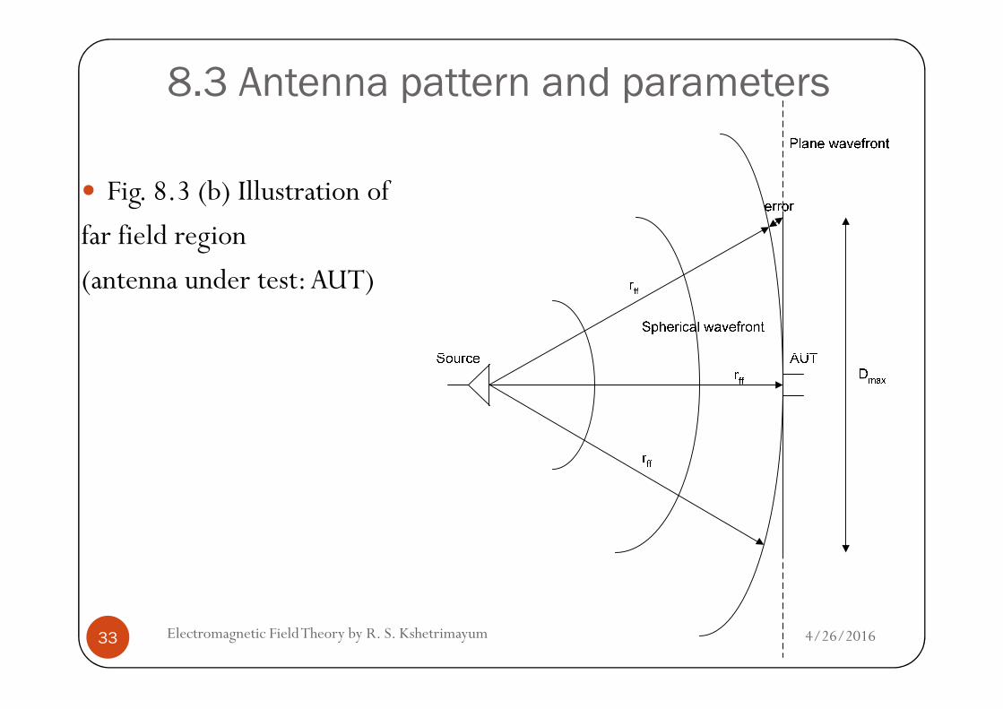
Fig. 8.3 (b) Illustration of
far field region
(antenna under test: AUT)
4/26/2016Electromagnetic Field Theory by R. S. Kshetrimayum33

8.3 Antenna pattern and parameters
We can calculate the distance rff by equating the maximum error (which is at the edges of the AUT of maximum dimension Dmax) in the distance r by approximating spherical wavefront to plane wavefront to λ/16 (Exercise 8.1)
8.3.2 Direction of the main beam (θmax)
4/26/2016Electromagnetic Field Theory by R. S. Kshetrimayum34
8.3.2 Direction of the main beam (θmax)
A radiation lobe is a clear peak in the radiation intensity surrounded by regions of weaker radiation intensity

8.3 Antenna pattern and parameters
Main beam is the biggest lobe in the radiation pattern of the antenna
It is the radiation lobe in the direction of maximum radiation
θmax is the direction in which maximum radiation occurs
Any lobe other than the main lobe is called as minor lobe
4/26/2016Electromagnetic Field Theory by R. S. Kshetrimayum35
Any lobe other than the main lobe is called as minor lobe
The radiation lobe opposite to the main lobe is also termed as back lobe This will be more appropriate for polar plot of radiation pattern

8.3 Antenna pattern and parameters
8.3.3 Half power beam width (HPBW)
It is the angular separation between the half of the maximum power radiation in the main beam
At these points, the radiation electric field reduces by of the maximum electric field
1
2
4/26/2016Electromagnetic Field Theory by R. S. Kshetrimayum36
of the maximum electric field
Half power is also equal to -3-dB
We also call HPBW as -3-dB beamwidth
They are measured in the E-plane and H-plane radiation patterns of the antenna
8.3 Antenna pattern and parameters
8.3.4 Beam width between first nulls (BWFN)
It is the angular separation between the first two nulls on either side of the main beam
For same values of BWFN, we can have different values of HPBW for narrow beams and broad beams
4/26/2016Electromagnetic Field Theory by R. S. Kshetrimayum37
HPBW for narrow beams and broad beams
HPBW is a better parameter for specifying the effective beam width
8.3 Antenna pattern and parameters
8.3.5 Side lobe level (SLL)
The side lobes are the lobes other than the main beam and it shows the direction of the unwanted radiation in the antenna
radiation pattern
The amplitude of the maximum side lobe in comparison to
4/26/2016Electromagnetic Field Theory by R. S. Kshetrimayum38
The amplitude of the maximum side lobe in comparison to the main beam maximum amplitude of the electric field is called as side lobe level (SLL)
It is normally expressed in dB and a SLL of -30 dB or less is considered to be good for a communication system
8.3 Antenna pattern and parameters
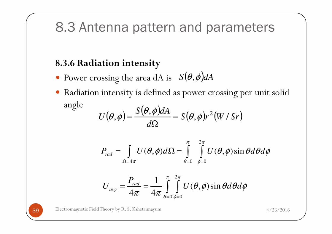
8.3.6 Radiation intensity
Power crossing the area dA is
Radiation intensity is defined as power crossing per unit solid angle
( )dAS φθ ,
( ) ( ) ( ) ( )SrWrSdAS
U /,,
, 2φθφθ
φθ ==
4/26/2016Electromagnetic Field Theory by R. S. Kshetrimayum39
2
4 0 0
( , ) ( , ) sinradP U d U d d
π π
π θ φ
θ φ θ φ θ θ φΩ= = =
= Ω =∫ ∫ ∫
2
0 0
1( , )sin
4 4
radavg
PU U d d
π π
θ φ
θ φ θ θ φπ π
= =
= = ∫ ∫
( ) ( ) ( )SrWrSd
U /,, φθφθ =Ω
=
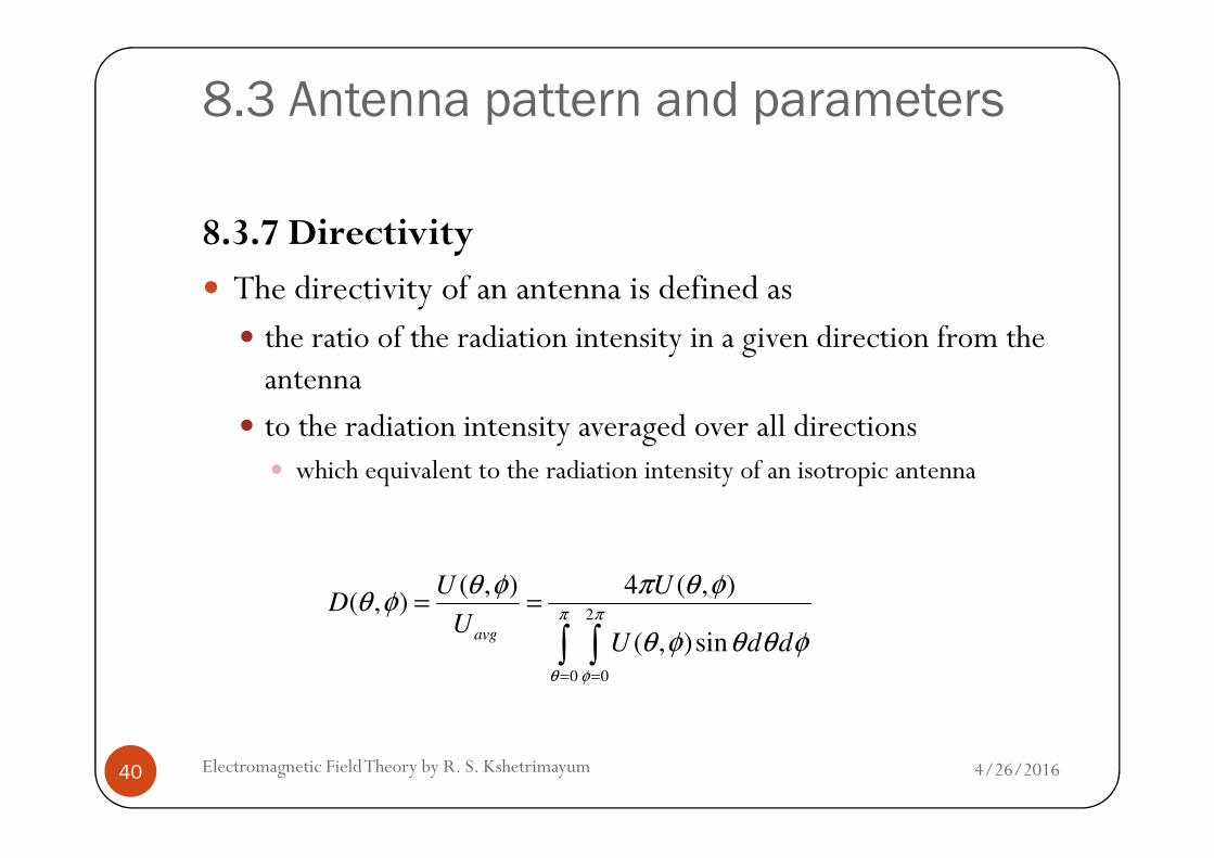
8.3 Antenna pattern and parameters
8.3.7 Directivity
The directivity of an antenna is defined as the ratio of the radiation intensity in a given direction from the
antenna
to the radiation intensity averaged over all directions
4/26/2016Electromagnetic Field Theory by R. S. Kshetrimayum40
to the radiation intensity averaged over all directions which equivalent to the radiation intensity of an isotropic antenna
2
0 0
( , ) 4 ( , )( , )
( , )sinavg
U UD
UU d d
π π
θ φ
θ φ π θ φθ φ
θ φ θ θ φ= =
= =
∫ ∫
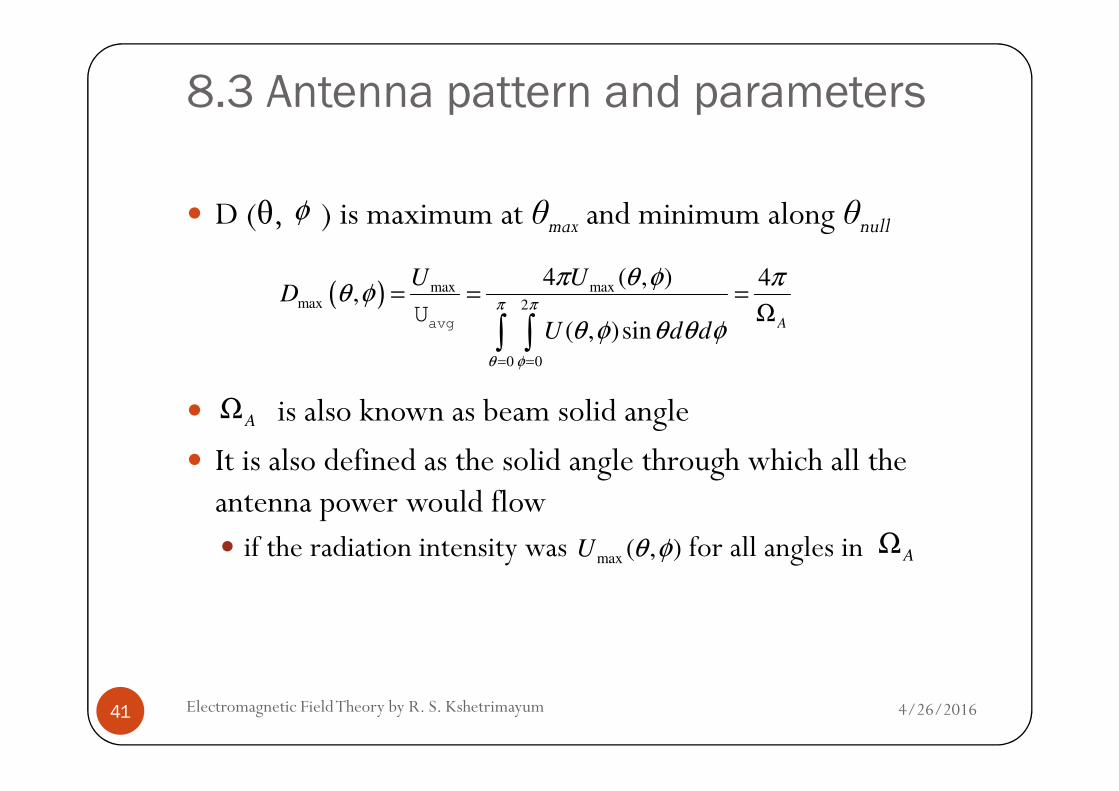
8.3 Antenna pattern and parameters
D (θ, ) is maximum at θmax and minimum along θnull
is also known as beam solid angle
φ
( ) max maxmax 2
0 0
4 ( , ) 4,
( , )sin A
U UD
U d d
π π
θ φ
π θ φ πθ φ
θ φ θ θ φ= =
= = =Ω
∫ ∫avgU
Ω
4/26/2016Electromagnetic Field Theory by R. S. Kshetrimayum41
is also known as beam solid angle
It is also defined as the solid angle through which all the antenna power would flow if the radiation intensity was for all angles in
AΩ
max ( , )U θ φ AΩ

8.3 Antenna pattern and parameters
Given an antenna with one narrow major beam, negligible radiation in its minor lobes
where and are the half-power beam widths in
HPBW HPBW
rad rad
A θ φΩ ≈ ×
θ φ
4/26/2016Electromagnetic Field Theory by R. S. Kshetrimayum42
where and are the half-power beam widths in radians which are perpendicular to each other
For narrow beam width antennas
It can be shown that the maximum directivity is given by
HPBWθHPBWφ
( ), 1HPBW HPBW
θ φ <<
max
4
HPBW HPBW
rad radD
π
θ φ≅
×

8.3 Antenna pattern and parameters
If the beam widths are in degrees, we have
8.3.8 Gain
2
max deg deg deg deg
1804
41,253
HPBW HPBW HPBW HPBW
D
ππ
θ φ θ φ
≅ =
× ×
4/26/2016Electromagnetic Field Theory by R. S. Kshetrimayum43
8.3.8 Gain
In defining directivity, we have assumed that the antenna is lossless
But, antennas are made of conductors and dielectrics

8.3 Antenna pattern and parameters
It has same in-built losses accompanied with the conductors and dielectrics
Thereby, the power input to the antenna is partly radiated and remaining part is lost in the imperfect conductors as well as in
4/26/2016Electromagnetic Field Theory by R. S. Kshetrimayum44
remaining part is lost in the imperfect conductors as well as in dielectrics
The gain of an antenna in a given direction is defined as the ratio of the intensity in a given direction
to the radiation intensity that would be obtained if the power accepted by the antenna were radiated isotropically

8.3 Antenna pattern and parameters
Note that definitions of the antenna directivity and gain are essentially the same
( ) radrad
4 ( , )e4 ( , ), e ( , )
input rad
UUG D
P P
π θ φπ θ φθ φ θ φ= = =
4/26/2016Electromagnetic Field Theory by R. S. Kshetrimayum45
essentially the same except for the power terms used in the definitions
Directivity is the ratio of the antenna radiated power density at a distant point to the total antenna radiated power radiated isotropically
Gain is the ratio of the antenna radiated power density at a distant point to the total antenna input power radiated isotropically
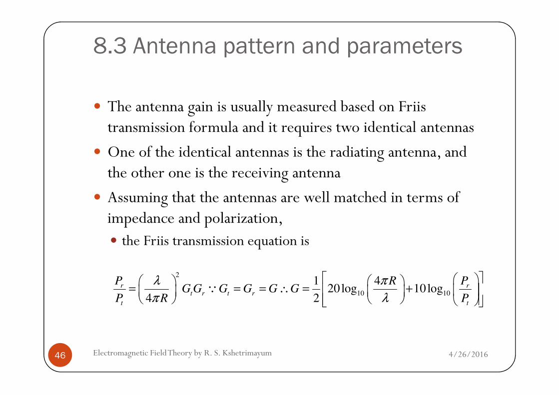
8.3 Antenna pattern and parameters
The antenna gain is usually measured based on Friistransmission formula and it requires two identical antennas
One of the identical antennas is the radiating antenna, and the other one is the receiving antenna
Assuming that the antennas are well matched in terms of
4/26/2016Electromagnetic Field Theory by R. S. Kshetrimayum46
Assuming that the antennas are well matched in terms of impedance and polarization, the Friis transmission equation is
2
10 10
1 420log 10log
4 2
r rt r t r
t t
P PRG G G G G G
P R P
λ π
π λ
= = = ∴ = +
Q

8.3 Antenna pattern and parameters
Friis transmission equation states that the ratio of the received power at the receiving antenna and transmitted power at the transmitting antenna is: directly proportional to both gains of the transmitting (Gt) and
receiving (Gr) antennas
4/26/2016Electromagnetic Field Theory by R. S. Kshetrimayum47
receiving (Gr) antennas
inversely proportional to square of the distance between the transmitting and receiving antennas (1/R2) and
directly proportional to the square of the wavelength of the signal transmitted (λ2)

8.3 Antenna pattern and parameters
Assumptions made are:
(a) antennas are placed in the far-field regions
(b) there is free space direct line of sight propagation between the two antennas
(c) there are no interferences from other sources and
4/26/2016Electromagnetic Field Theory by R. S. Kshetrimayum48
(c) there are no interferences from other sources and no multipaths between the transmitting and receiving antennas
due to reflection,
refraction and
diffraction

8.3 Antenna pattern and parameters
8.3.9 Polarization
Let us consider antenna is placed at the origin of a spherical coordinate system and wave is propagating radially outward in all directions
In the far field region of an antenna,
4/26/2016Electromagnetic Field Theory by R. S. Kshetrimayum49
In the far field region of an antenna,
( ) ( ) ( )ˆ ˆ, , ,E E Eθ φθ φ θ φ θ θ φ φ= +r

8.3 Antenna pattern and parameters
Putting the time dependence, we have,
where δ is the phase difference between the elevation and azimuthal components of the electric field
( ) ( ) ( ) ( ) ( ) ( ) ( )ˆ ˆ ˆ ˆ, , , cos , cos , , , ,E t E t E t E t E tθ φ θ φθ φ θ φ ω θ θ φ ω δ φ θ φ θ θ φ φ= + + = +r
4/26/2016Electromagnetic Field Theory by R. S. Kshetrimayum50
azimuthal components of the electric field
The figure traced out by the tip of the radiated electric field vector as a function of time for a fixed position of space can be defined
as antenna polarization

8.3 Antenna pattern and parameters
a) LP
When δ=0, the two transversal electric field components are in time phase
The total electric field vector
4/26/2016Electromagnetic Field Theory by R. S. Kshetrimayum51
makes an angle with the -axis
( ) ( ) ( ) ( ) ( )( )ˆ ˆ, , , cos , cosE t E t E tθ φθ φ θ φ ω θ θ φ ω φ= +r
LPθ θ
( )( )
( )( )
1 1, , , ,
tan tan, , , ,
LP
E t E t
E t E t
φ φ
θ θ
θ φ θ φθ
θ φ θ φ− −
= =
8.3 Antenna pattern and parameters
The tip of the total radiated electric field vector traces out a line
Therefore, the antenna’s polarization is LP
b) CP
When , the two transversal electric field components πδ = ±
4/26/2016Electromagnetic Field Theory by R. S. Kshetrimayum52
When , the two transversal electric field components are out of phase in time
and if the two transversal electric field components are of equal amplitude
2
πδ = ±
( ) ( ) ( )0, , ,E E Eθ φθ φ θ φ θ φ= =

8.3 Antenna pattern and parameters
The total electric field vector
makes an angle with the -axis
( ) ( ) ( ) ( ) ( )( )ˆ ˆ, , , cos , sinE t E t E tθ φθ φ θ φ ω θ θ φ ω φ= +r
CPθ θ
4/26/2016Electromagnetic Field Theory by R. S. Kshetrimayum53
This implies that the total radiated electric field vector of the antenna traces out a circle as time progresses from 0 to 2 and so on
( )( )
( )1 1sin
tan tan tancos
CP
tt t
t
ωφ ω ω
ω− −
= = =
π
ω
8.3 Antenna pattern and parameters
If the vector rotates counterclockwise (clockwise), then the antenna polarization is RHCP (LHCP)
For
the total electric field vector traces out an ellipse and
( ) ( ), , 0,E E andθ φθ φ θ φ α π≠ ≠ πδ ,0≠
4/26/2016Electromagnetic Field Theory by R. S. Kshetrimayum54
the total electric field vector traces out an ellipse and hence it is elliptically polarized (EP)
The ratio of the major and minor axes of the ellipse is called axial ratio (AR)
For instance, AR=0 dB for CP and AR= ∞ dB for LP
8.3 Antenna pattern and parameters
Let us try to understand two terms (co- and cross-polarization) which are important for the antenna radiation pattern
Co-polarization means you measure the antenna with another antenna oriented in the same polarization with the antenna
4/26/2016Electromagnetic Field Theory by R. S. Kshetrimayum55
antenna oriented in the same polarization with the antenna under test (AUT)
Cross-polarization means that you measure the antenna with antenna oriented perpendicular w.r.t. the main polarization

8.3 Antenna pattern and parameters
Cross-polarization is the polarization orthogonal to the polarization under consideration
For example, if the field of an antenna is horizontally polarized, the cross-polarization for this case is vertical polarization
4/26/2016Electromagnetic Field Theory by R. S. Kshetrimayum56
polarization
If the polarization is RHCP, the cross-polarization is LHCP
Let us put this into mathematical expressions:
We may write the total electric field propagating along z-axis as
( )ˆ ˆ j z
co co cr crE E u E u e
β−= +r

8.3 Antenna pattern and parameters
where the co- and cross-polarization unit vectors satisfy the orthonormality condition
Therefore, the co- and cross-polarization components of the
* * * *ˆ ˆ ˆ ˆ ˆ ˆ ˆ ˆ1, 1, 0, 0co co cr cr co cr cr co
u u u u u u u u• = • = • = • =
4/26/2016Electromagnetic Field Theory by R. S. Kshetrimayum57
Therefore, the co- and cross-polarization components of the electric fields can be obtained as
* *ˆ ˆ,co co cr crE E u E E u= • = •r r

8.3 Antenna pattern and parameters
a) LP
For a general LP wave, we can write,
For a x-directed LP wave, =0, hence,
ˆ ˆ ˆ ˆ ˆ ˆcos sin , sin cosco LP LP cr LP LP
u x y u x yφ φ φ φ= + = −
LPφ
4/26/2016Electromagnetic Field Theory by R. S. Kshetrimayum58
For a y-directed LP wave, =900, hence,
* *ˆ ˆ ˆ ˆ ˆ ˆ, ; ,co cr co co x cr cr y
u x u y E E u E E E u E= = − = • = = • = −r r
LPφ
* *ˆ ˆ ˆ ˆ ˆ ˆ, ; ,co cr co co y cr cr xu y u x E E u E E E u E= = = • = = • =r r

8.3 Antenna pattern and parameters
b) CP
For a RHCP wave, we can write,
ˆ ˆ ˆ ˆˆ ˆ,
2 2co cr
x jy x jyu u
− += =
4/26/2016Electromagnetic Field Theory by R. S. Kshetrimayum59
For a LHCP wave, co- and cross-polarization unit vectors and components of the electric field will interchange
* *ˆ ˆ,2 2
x y x y
co co cr cr
E jE E jEE E u E E u
+ −= • = = • =r r

8.3 Antenna pattern and parameters
c) EP
For a EP wave, we can write,
2 2
ˆ ˆ ˆ ˆˆ ˆ,
1 1
EP EPj j
co cr
x Ae y Ae x yu u
A A
φ φ−+ − += =
+ +
4/26/2016Electromagnetic Field Theory by R. S. Kshetrimayum60
In order to determine the far-field radiation pattern of an AUT, two antennas are required
The one being tested (AUT) is normally free to rotate and it is connected in receiving mode

8.3 Antenna pattern and parameters
4/26/2016Electromagnetic Field Theory by R. S. Kshetrimayum61

8.3 Antenna pattern and parameters
Note that AUT as a receiving antenna measurement will generate the same radiation pattern to that of AUT used as a transmitting antenna (from reciprocity theorem)
Another antenna is usually fixed and it is connected in transmitting mode
4/26/2016Electromagnetic Field Theory by R. S. Kshetrimayum62
transmitting mode
The AUT is rotated by a positioner and it can rotate 1-, 2-and 3-degrees of freedom of rotation

8.3 Antenna pattern and parameters
The AUT is rotated in usually two principal planes (elevation and azimuthal)
The received field strength is measured by a spectrum analyzer or power meter which will be used to generate the antenna radiation pattern in
4/26/2016Electromagnetic Field Theory by R. S. Kshetrimayum63
which will be used to generate the antenna radiation pattern in two principal planes also known as E- and H- planes
The antenna radiation patterns in these two principal planes can be used to generate the 3-D radiation pattern of an antenna

8.3 Antenna pattern and parameters
4/26/2016Electromagnetic Field Theory by R. S. Kshetrimayum64
Equivalent circuit of an antenna

8.3 Antenna pattern and parameters
8.3.10 Quality factor and bandwidth
The equivalent circuit of a resonant antenna can be approximated by a series RLC resonant circuit
where R=Rr+RL are the radiation and loss resistances,
4/26/2016Electromagnetic Field Theory by R. S. Kshetrimayum65
L is the inductance and
C is the capacitance of the antenna

8.3 Antenna pattern and parameters
For a resonant antenna like dipoles, the FBW is related to the radiation efficiency and quality factor Q (FBW=1/Q)
The quality factor of an antenna is defined as 2πf0 (f0 is the resonant frequency) times the energy stored over the
4/26/2016Electromagnetic Field Theory by R. S. Kshetrimayum66
the resonant frequency) times the energy stored over the power radiated and Ohmic losses
( )
( ) ( )
( )
2 2
2
0 00
20
0
1 1 1
4 4 2 2 12
1 2
2
1
2
r L r Lr L
rlossless rad
r r L
I L If L f L
Q fR R f R R C
I R R
RQ e
f R C R R
π ππ
π
π
+
= = =+ ++
= = •+
8.3 Antenna pattern and parameters
where Qlossless is the quality factor when the antenna is lossless (RL=0) and
erad is the antenna radiation efficiency.
Note that the radiation efficiency of an antenna is defined as the ratio of the power delivered to the radiation resistance Rr
4/26/2016Electromagnetic Field Theory by R. S. Kshetrimayum67
the ratio of the power delivered to the radiation resistance Rr
to the power delivered to Rr and RL
( ) ( )
2
2
1
21
2
rr
rad
r Lr L
I RR
eR R
I R R
= =++
8.3 Antenna pattern and parameters
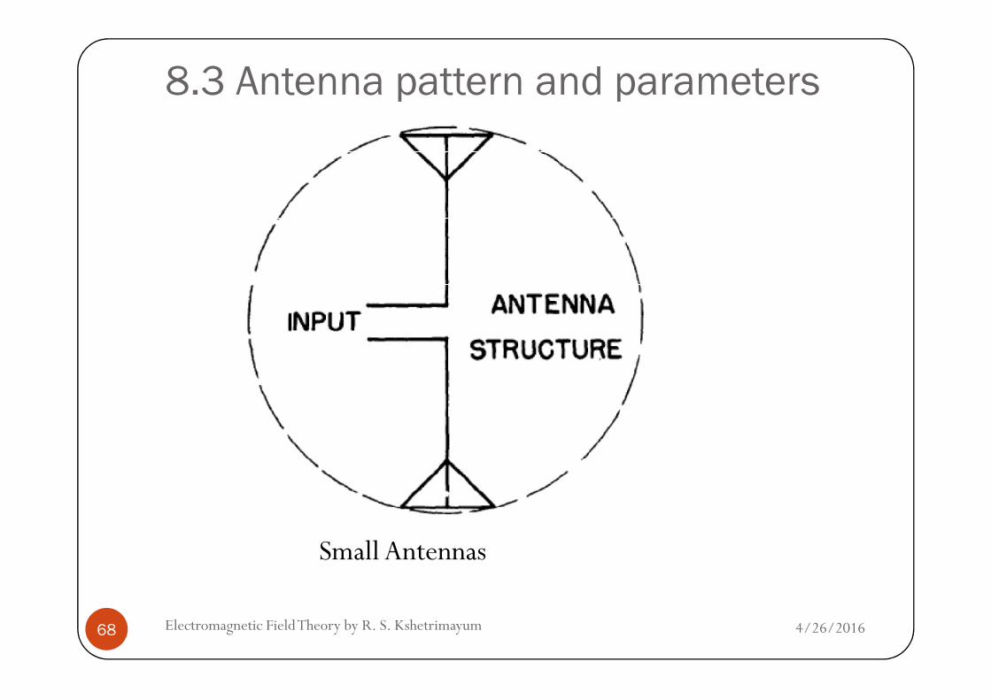
4/26/2016Electromagnetic Field Theory by R. S. Kshetrimayum68
Small Antennas
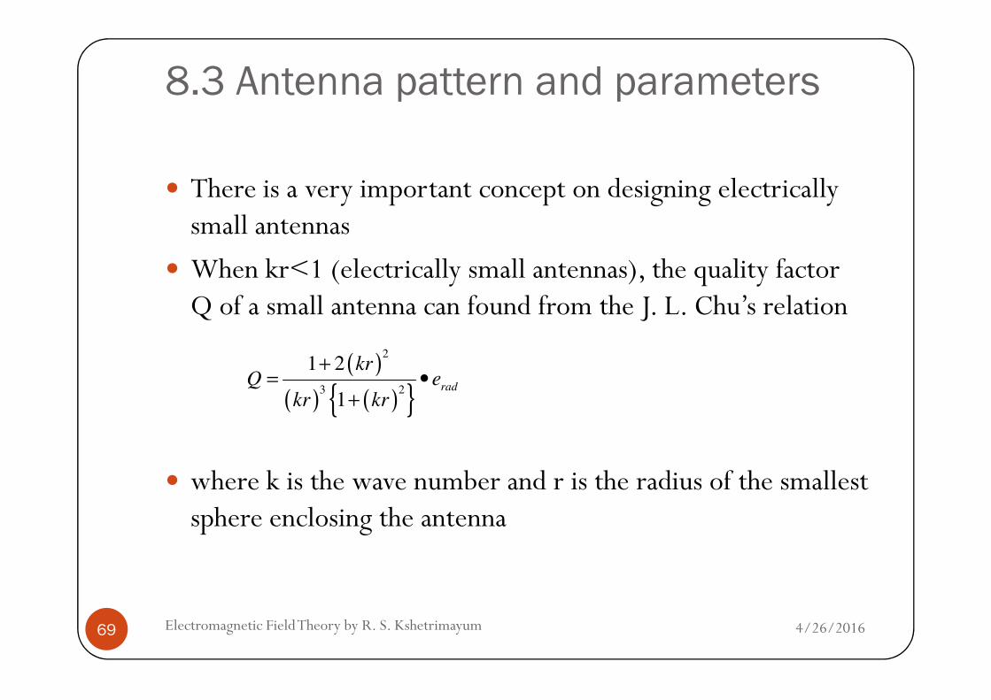
8.3 Antenna pattern and parameters
There is a very important concept on designing electrically small antennas
When kr<1 (electrically small antennas), the quality factor Q of a small antenna can found from the J. L. Chu’s relation
( )2
+
4/26/2016Electromagnetic Field Theory by R. S. Kshetrimayum69
where k is the wave number and r is the radius of the smallest sphere enclosing the antenna
( )
( ) ( )
2
3 2
1 2
1rad
krQ e
kr kr
+= •
+

8.3 Antenna pattern and parameters
The above relation gives the relationship between the antenna size, efficiency and quality factor.
This expression can be reduced further for smallest Q for a LP very small antenna (kr<<1) as follows:
4/26/2016Electromagnetic Field Theory by R. S. Kshetrimayum70
Harrington gave also a practical upper limit to the gain of a small antenna for a reasonable BW as
( )min 3
1 1Q
krkr= +
( ) ( )2
max 2G kr kr= +
8.3 Antenna pattern and parameters
For example, for a Hertz dipole of very small length 0.01λ, Qmin =32283
It has very high Q and hence a very narrow FBW (0.000031)
Gmax=0.0638 or -12dB
Note that in the above calculations r=0.005λ has been used
4/26/2016Electromagnetic Field Theory by R. S. Kshetrimayum71
Note that in the above calculations r=0.005λ has been used
But the gain of the antenna in dB is also negative
Antenna size, quality factor, bandwidth and radiation efficiency is interlinked
There is no complete freedom to optimize each one of them independently

8.3 Antenna pattern and parametersRECAP:
Antenna acts as an interface between a guided wave and a
free-space wave
One of the most important characteristics of an antenna is its
directional property
Ability to concentrate radiated power in a certain directionAbility to concentrate radiated power in a certain direction
Or receive power from a preferred direction
This directional property is characterized in Radiation pattern
From reciprocity theorem, we can show that
the pattern characteristics of an antenna are the same in the
transmit and
the receive modes

8.3 Antenna pattern and parameters
FeedLine Antenna
Source
Radiated fields

8.3 Antenna pattern and parameters
A plot of electric or magnetic field intensity as function of the direction at a constant distance from the antenna is known as the electric field pattern or magnetic field pattern
The field intensity along a direction (θ,φ) is given by the length of the position vector to a point on the surface of the 3D shape in the direction (θ,φ)
4/26/2016Electromagnetic Field Theory by R. S. Kshetrimayum74
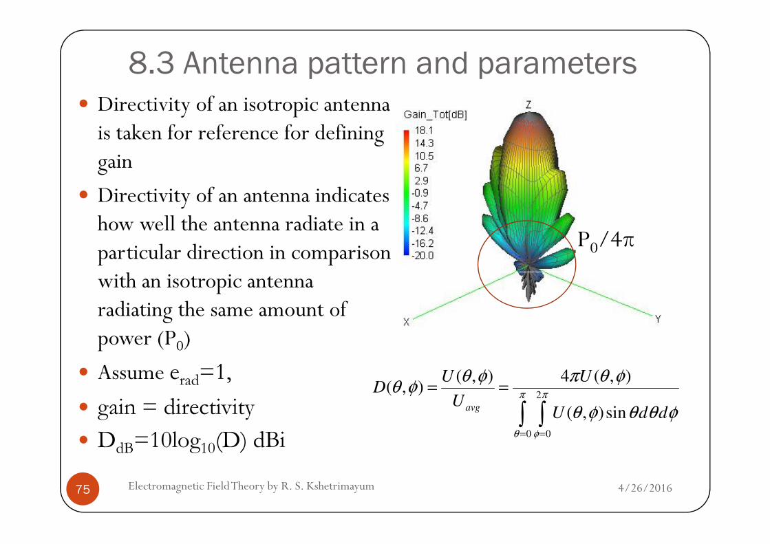
8.3 Antenna pattern and parameters Directivity of an isotropic antenna
is taken for reference for defining gain
Directivity of an antenna indicates how well the antenna radiate in a particular direction in comparison with an isotropic antenna
P0/4π
4/26/2016Electromagnetic Field Theory by R. S. Kshetrimayum75
with an isotropic antenna radiating the same amount of power (P0)
Assume erad=1,
gain = directivity
DdB=10log10(D) dBi
2
0 0
( , ) 4 ( , )( , )
( , )sinavg
U UD
UU d d
π π
θ φ
θ φ π θ φθ φ
θ φ θ θ φ= =
= =
∫ ∫
8.3 Antenna pattern and parameters
Generally single value of gain or directivity is given in that case the gain or directivity is along the main beam peak
Antenna equivalent circuit can be thought of as Radiation resistance
Loss resistance
4/26/2016Electromagnetic Field Theory by R. S. Kshetrimayum76
Loss resistance
Reactive parts
So the feed line also has a characteristic impedance Z0 usually of 50 Ohm
At the input of the antenna, the impedance seen by the feed line can be assumed as ZL

8.3 Antenna pattern and parameters
Then the reflection coefficient and VSWR may be calculated as
2:
1,10
1
1;
0
0
≤
∞≤≤≤Γ≤
Γ−
Γ+=
+
−=Γ
VSWRBW
VSWR
VSWRZZ
ZZ
L
L
4/26/2016Electromagnetic Field Theory by R. S. Kshetrimayum77
Polarization of the antenna is the polarization of the wave radiated by the antenna in the far field
Polarization of the antenna is direction-dependent
Conventionally polarization of the wave is along the main beam direction

8.3 Antenna pattern and parameters
Received signal power in a wireless communication link
The received signal power is a function of four elements: The transmitter output electrical power (pT)
The fraction of the transmitter electrical power directed at the receiver defined by the transmit antenna gain (gT)
4/26/2016Electromagnetic Field Theory by R. S. Kshetrimayum78
receiver defined by the transmit antenna gain (gT)
The loss of energy in the communication medium
The fraction of the received electrical power directed at the receiver defined by the received antenna gain (gR)

8.3 Antenna pattern and parameters
Power flux density (pfd) for isotropic radiator at a distance r =p0/(4πr2)
Power transmitted= pT gT
pfd= pT gT /(4πr2)
In dB,
4/26/2016Electromagnetic Field Theory by R. S. Kshetrimayum79
In dB,
PFD= PT +GT-10log4πr2=EIRP-10log4πr2 (dBW/m2)
where equivalent isotropic radiated power=EIRP
No matter what, a large portion of the transmitted energy 10log4πr2 is not seen by the receiver
8.3 Antenna pattern and parameters
The received power at the receiver antenna is
Pr=pfd×Aer
Effective aperture is defined as the ratio of power delivered to the load if antenna to the Poynting vector in any direction (θ,φ)
4/26/2016Electromagnetic Field Theory by R. S. Kshetrimayum80
(θ,φ)
Ae (θ,φ) =Pr (θ,φ) /S (m2)
Note that for any antenna it can be shown that
G/Ae=(4×π)/λ2
Or, Ae=G λ2 /(4×π)

8.3 Antenna pattern and parameters
Pr=pfd×Ae= pT gTgr λ2 /(4×πr)2
PR=PT+GT+GR-20log((4×πr) ×c/f) (dBW)
The last term is called range loss or power loss between two isotropic antennas at particular range and frequency
4/26/2016Electromagnetic Field Theory by R. S. Kshetrimayum81
8.4 Kinds of antennas8.4.1 Hertz dipole
Let us find the fields of a small current carrying element of length dl
An infinitesimally small current element is called a Hertz dipole
4/26/2016Electromagnetic Field Theory by R. S. Kshetrimayum82
Hertz dipole
Electrically small antennas are small relative to wavelength
Whereas electrically large antennas are large relative to wavelength
Hertz dipole is not of much practical use but it is the basic building block of any kind of antennas

8.4 Kinds of antennas The infinitesimal time-varying current in the Hertz dipole is
where ω is the angular frequency of the current
Since the current is assumed along the z-direction, the
( ) zeItI tj ˆ0ω=
4/26/2016Electromagnetic Field Theory by R. S. Kshetrimayum83
Since the current is assumed along the z-direction, the magnetic vector potential at the observation point P is along z-direction (see section 3.10)
zr
edleIzAA
tjrj
z ˆ4
ˆ 00
π
µ ωβ−
==r
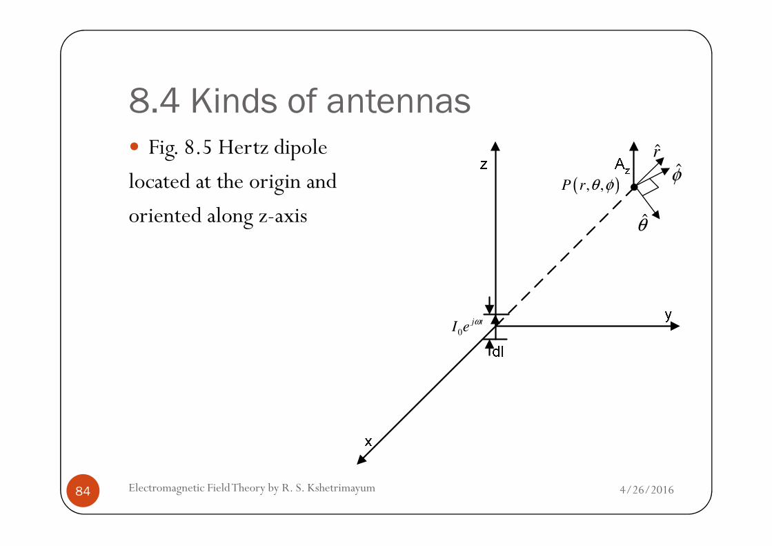
8.4 Kinds of antennas Fig. 8.5 Hertz dipole
located at the origin and
oriented along z-axis ( ), ,P r θ φ
r
θ
φ
4/26/2016Electromagnetic Field Theory by R. S. Kshetrimayum84
0
j tI e
ω

8.4 Kinds of antennas Note that for this case
For infinitesimally small current element at the origin
using the coordinate transformation from the Rectangular to Spherical coordinate systems (see section 1.3.3)
( )' '
0
j tJ r dv I dle
ω=r r
'r r r− =r r r
4/26/2016Electromagnetic Field Theory by R. S. Kshetrimayum85
Spherical coordinate systems (see section 1.3.3)
sin cos sin sin cos sin cos sin sin cos 0
cos cos cos sin sin cos cos cos sin sin 0
sin cos 0 sin cos 0
xr
y
zz
AA
A A
AA A
θ
φ
θ φ θ φ θ θ φ θ φ θ
θ φ θ φ θ θ φ θ φ θ
φ φ φ φ
= − = − − −
cos ; sin ; 0r z zA A A A Aθ φθ θ⇒ = = − =
8.4 Kinds of antennas
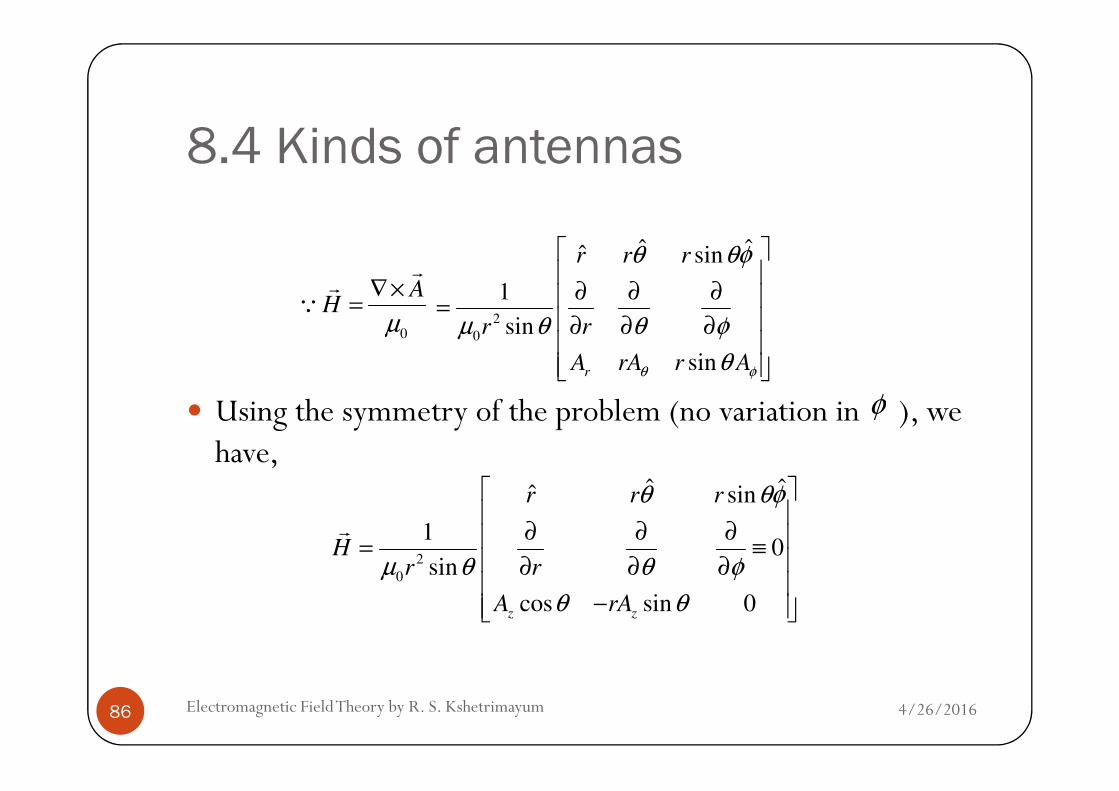
Using the symmetry of the problem (no variation in ), we
0
AH
µ
∇×=
rr
Q2
0
ˆ ˆˆ sin
1
sin
sinr
r r r
r r
A rA r Aθ φ
θ θφ
µ θ θ φ
θ
∂ ∂ ∂ = ∂ ∂ ∂
φ
4/26/2016Electromagnetic Field Theory by R. S. Kshetrimayum86
Using the symmetry of the problem (no variation in ), we have,
2
0
ˆ ˆˆ sin
10
sin
cos sin 0z z
r r r
Hr r
A rA
θ θφ
µ θ θ φ
θ θ
∂ ∂ ∂ = ≡ ∂ ∂ ∂
−
r
φ

8.4 Kinds of antennas
( ) ( )2
0
sin0; 0; sin cos
sinr z z
rH H H rA A
r rθ φ
θθ θ
µ θ θ
∂ ∂ ⇒ = = = − −
∂ ∂
( )0 0ˆ ˆcos sin
sin sin4 4
j t j tj r j rj r j rI dle I dlee e
H e j er r r r r
ω ωβ ββ β
φ
φ φθ θθ β θ
π θ π
+ +− −− −
∂ ∂ ⇒ = − − = +
∂ ∂
4/26/2016Electromagnetic Field Theory by R. S. Kshetrimayum87
The Hertz dipole has only component of the magnetic field, i.e., the magnetic field circulates the dipole
0
2
ˆ sin 1
4
j t j rI dle e j
r r
ω βφ θ β
π
+ − = +
φ

8.4 Kinds of antennas The electric field for ( in free space, we don’t have
any conduction current flowing) can be obtained as
Using the symmetry of the problem (no variation in ) like
0J =r
ωεj
HE
rr ×∇
=
φ
4/26/2016Electromagnetic Field Theory by R. S. Kshetrimayum88
Using the symmetry of the problem (no variation in ) like before, we have,
φ
( ) ( )2 2
ˆ ˆˆ sin
1 1 ˆˆ0 sin sinsin sin
0 0 sin
r r r
E r H r r H rj r r j r r
r H
φ φ
φ
θ θφ
θ θ θωε θ θ φ ωε θ θ
θ
∂ ∂ ∂ ∂ ∂ = ≡ = − ∂ ∂ ∂ ∂ ∂
r

8.4 Kinds of antennas
Note that Er has only 1/r2 and 1/r3 variation with r
( )20 0
2 2 2 2
1 1sin 2sin cos
sin 4 sin 4
j t j r j t j r
r
I dle e I dle ej jE r r
j r r r j r r r
ω β ω ββ βθ θ θ
ωε θ π θ ωε θ π
− −∂ = + = +
∂
( )
+∂
∂−=
∂
∂−= − rj
tj
er
jrrj
dleIHr
rrj
rE
βω
φθ βπωε
θθ
θωε
1
4
sinsin
sin
0
2
4/26/2016Electromagnetic Field Theory by R. S. Kshetrimayum89
We see that electric field is in the (r, θ) plane whereas the magnetic field has component only
rj θωε sin
2
0
2 3
sin
4
j tj rI dle j j
er r r
ωβθ β β
πε ω ω ω−
= + −
φ

8.4 Kinds of antennas Therefore, the electric field and magnetic field are
perpendicular to each other (Which wave is this?)
Points to be noted:
1) Fields can be classified into three categories
(a) Radiation fields (spatial variation 1/r)
4/26/2016Electromagnetic Field Theory by R. S. Kshetrimayum90
(a) Radiation fields (spatial variation 1/r)
(b) Induction fields (spatial variation 1/r2) and
(c) Electrostatic fields (spatial variation 1/r3)

8.4 Kinds of antennas 2) Field variation with f since
a) Electrostatic fields (1/r3) are also inversely proportional to the frequency ( )
b) Induction field (1/r2) is independent of frequency ( )
µεωβ =
β
ω
1
4/26/2016Electromagnetic Field Theory by R. S. Kshetrimayum91
b) Induction field (1/r2) is independent of frequency ( )
c) Radiation field (1/r) is proportional to frequency ( )ω
β 2
ω
β

8.4 Kinds of antennas 2) Field variation with r
For small values of r, electrostatic field is the dominant term and
For large values of r,
radiation field is the dominant term
4/26/2016Electromagnetic Field Theory by R. S. Kshetrimayum92
radiation field is the dominant term
We can also observe that the three types of fields are equal in magnitude when
β2/r= β/r2=1/r3 => r=1/β= λ/2

8.4 Kinds of antennas For r< λ/2, 1/r3 term dominates
For r>> λ/2, the 1/r term dominates
Near field region:
For r<< λ/2
(in fact the near field region distance r= λ/2 is for D<<λ
4/26/2016Electromagnetic Field Theory by R. S. Kshetrimayum93
(in fact the near field region distance r= λ/2 is for D<<λfor an ideal infinitesimally small Hertz dipole
and the near field region distance for is for D>>λ), electrostatic fields dominate
3
0.62D
rλ
=

8.4 Kinds of antennas as r<< λ/2
1→− rje
βQ
0
3
cos2 ;
4
j t
r
I dl eE j
r
ωθ
πεω≈ − 0
3
sin
4
j tI dl eE j
r
ω
θ
θ
πεω≈ −
4/26/2016Electromagnetic Field Theory by R. S. Kshetrimayum94
The magnitude of the near field is
4 rπεω 4 rπεω
2 2 2 20
34cos sin
4r
I dlE E E
rθ θ θ
πεω= + = +

8.4 Kinds of antennas A polar plot of the near field can be generated by writing a
MATLAB program for plotting
Maximum field is along θ=00, θ=1800 and minimum is along
( ) θθθ 22 sincos4 +=F
4/26/2016Electromagnetic Field Theory by R. S. Kshetrimayum95
Maximum field is along θ=00, θ=1800 and minimum is along θ=900, θ=2700 (see Fig. 8.6(a))

8.4 Kinds of antennas
4/26/2016Electromagnetic Field Theory by R. S. Kshetrimayum96
Fig. 8.6 (a) Near field pattern plot of a Hertz dipole located at the origin and oriented along z-axis (maximum radiation along z-axis)

8.4 Kinds of antennas Far field region:
For r>> λ/2 (in between reactive near field and Fraunhofer far field region, there exists the Fresnel near field region that’s why we have chosen an r>> λ/2), radiation field is the dominant term
4/26/2016Electromagnetic Field Theory by R. S. Kshetrimayum97
field is the dominant term
In other words kr>>1, we have,
2
0 0sin sin;
4 4
j t j r j t j rI dl e e I dl e eE j H j
r r
ω β ω β
θ φ
θ β θ β
πεω π
− −
= =

8.4 Kinds of antennas The electric fields and magnetic fields are in phase with each
other
They are 90˚ out of phase with the current due to the (j) term in the expressions of Eθ and Hφ
It is interesting to note that the ratio of electric field and
4/26/2016Electromagnetic Field Theory by R. S. Kshetrimayum98
It is interesting to note that the ratio of electric field and magnetic field is constant
E
H
θ
φ
ω µεβ µη
ωε ωε ε= = = =

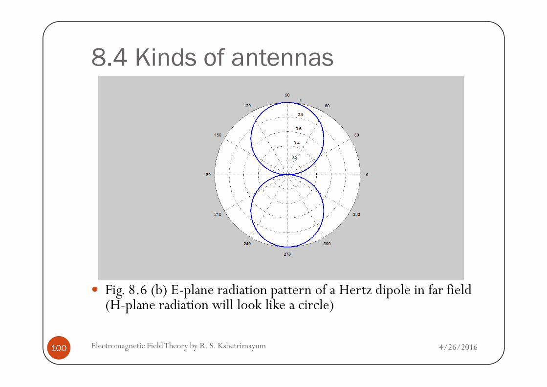
8.4 Kinds of antennas Hence, the fields have sinusoidal variations with θ
They are zero along θ=0
No radiation along z-axis unlike near field case
They are maximum along θ=π /2 (see Fig. 8.6 (b))
4/26/2016Electromagnetic Field Theory by R. S. Kshetrimayum99
8.4 Kinds of antennas
4/26/2016Electromagnetic Field Theory by R. S. Kshetrimayum100
Fig. 8.6 (b) E-plane radiation pattern of a Hertz dipole in far field (H-plane radiation will look like a circle)

8.4 Kinds of antennas Power flow:
( ) * *1 1 ˆ ˆˆRe Re2 2
avg rS E H E r E Hθ ϕθ φ= × = + ×r r
*1Re
2avgS E H rθ φ= $
2 3
0 sin1 I dlr
θ β =
$
4/26/2016Electromagnetic Field Theory by R. S. Kshetrimayum101
Antenna power flows radially outward Power density is not same in all directions The net real power is only due to the radiations fields (i.e.
jβ2/r and jβ/r) of electric and magnetic fields
Re2
avgS E H rθ φ=2 4
rrπ ωε
=
$

8.4 Kinds of antennas In the far field, electric field is along direction
magnetic field is along direction
Both of them are perpendicular to the power flow (Poyntingvector) which is along direction
Total radiated power:
θ
φ
r$
4/26/2016Electromagnetic Field Theory by R. S. Kshetrimayum102
Total radiated power:
The total radiated power from a Hertz dipole
2 sinavgW S r d dθ θ φ= ∫∫2
2 2
040dl
W Iπλ
∴ =

8.4 Kinds of antennas Power radiated by the Hertz dipole is proportional to
the square of the dipole length and
inversely proportional to the dipole wavelength
It implies more and more power is radiated as the frequency and
4/26/2016Electromagnetic Field Theory by R. S. Kshetrimayum103
the frequency and
the length
of the Hertz dipole increases
Radiation resistance of a Hertz Dipole:
Hertz dipole can be equivalently modeled as a radiation resistance

8.4 Kinds of antennasSince W=1/2 I0
2 Rrad
implies that Rrad = 80π2
Radiation pattern of a Hertz Dipole:
2
2 2
040dl
W Iπλ
∴ =
2dl
λ
4/26/2016Electromagnetic Field Theory by R. S. Kshetrimayum104
Radiation pattern of a Hertz Dipole:
F(θ, )=sin θ for a Hertz dipole
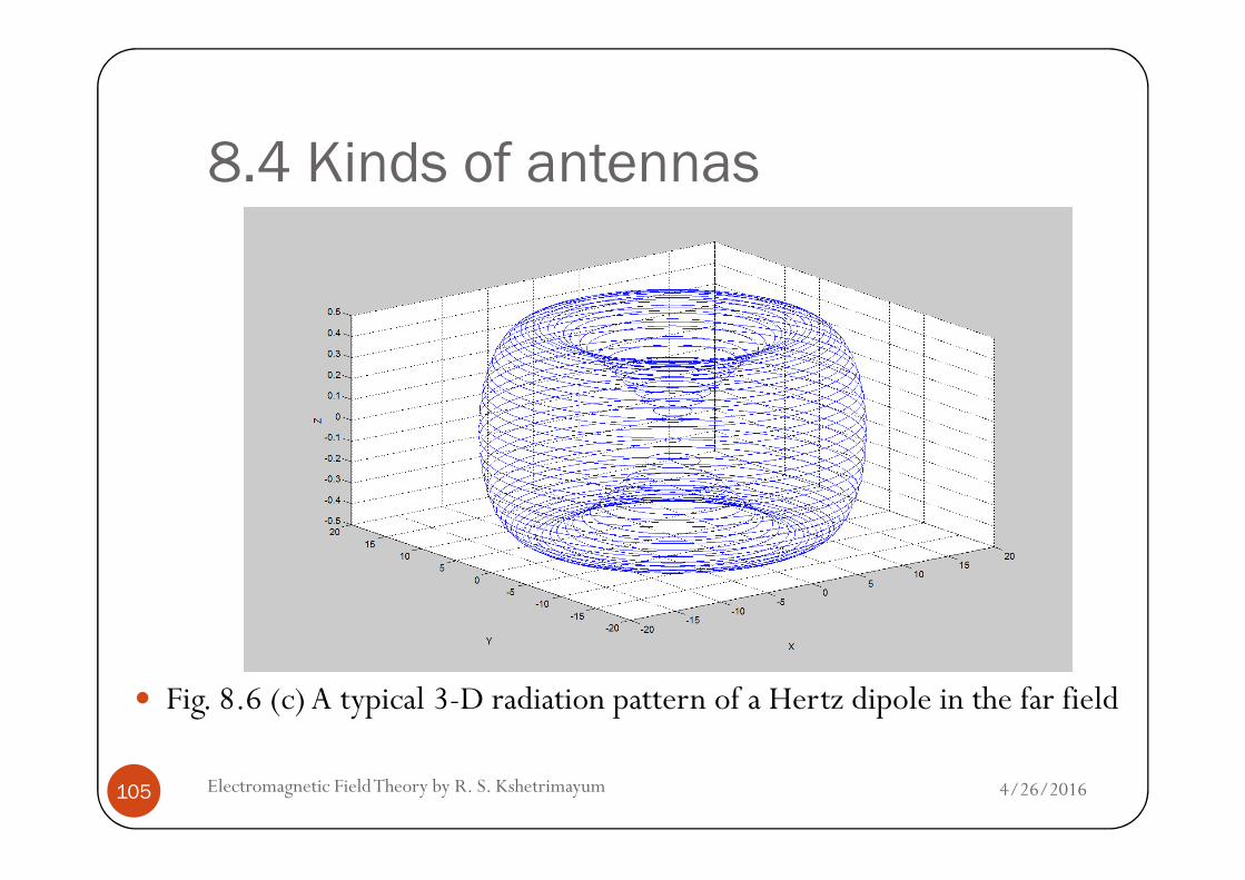
The 3D plot of sin θ looks like an apple (see Figure 8.6 (c))
8.4 Kinds of antennas
4/26/2016Electromagnetic Field Theory by R. S. Kshetrimayum105
Fig. 8.6 (c) A typical 3-D radiation pattern of a Hertz dipole in the far field
8.4 Kinds of antennas To get the 3-D plot from the 2-D plot you need to rotate the
E-plane pattern along the H-plane pattern
For this case it will give the shape of an apple
Note that θ is also known as elevation angle and as azimuth angle
φ
4/26/2016Electromagnetic Field Theory by R. S. Kshetrimayum106
azimuth angle
E-plane pattern for a dipole is also known as elevation pattern
H-plane pattern as azimuthal pattern

8.4 Kinds of antennas As mentioned before, it is easier to visualize 2-D plots than
3-D on a 2-D plane like pages of this book
Two principal planes radiation patterns are normally plotted E-plane (vertical: all planes containing z-axis like xz-plane, yz-
plane)
4/26/2016Electromagnetic Field Theory by R. S. Kshetrimayum107
plane)
H-plane (horizontal) radiations patterns
are sufficient to describe the radiation pattern of a Hertz dipole
H-plane (xy-plane) radiation pattern is in the form of circle of radius 1 since F(θ, ) is independent of φ φ

8.4 Kinds of antennas Since the ratio of electric and magnetic field amplitudes in
the far field region of an antenna is 377 Ohm We may also plot the power pattern instead of field pattern
from the relation p(θ, )=sin2 θ
Polarization of Hertz dipole:
4/26/2016Electromagnetic Field Theory by R. S. Kshetrimayum108
In the far-field region of a Hertz dipole, only θ component of the electric field the electric field is LP along direction
That means electric field is perpendicular to the line from the center of the dipole to the field observation point (see Fig. 8.5) and it lies in the plane containing this line and the dipole axis
θ

8.4 Kinds of antennas8.4.2 Dipole antenna
The next extension of a Hertz dipole is a linear antenna or a dipole of finite length as depicted in Fig. 8.7 (a)
It consists of a conductor of length 2L fed by a voltage or current source at its center
4/26/2016Electromagnetic Field Theory by R. S. Kshetrimayum109
current source at its center
The current distribution can be obtained by assuming an o.c. transmission line
For o.c. transmission line
( )0 0
0 0
( ) 2 sinj z j zV VI z e e j z
Z Z
β β β+ +
− += − = −

8.4 Kinds of antennas
θ
4/26/2016Electromagnetic Field Theory by R. S. Kshetrimayum110
Fig. 8.7 (a) Dipole of length
2L (Dipole can be assumed
to composed of many Hertz dipoles)
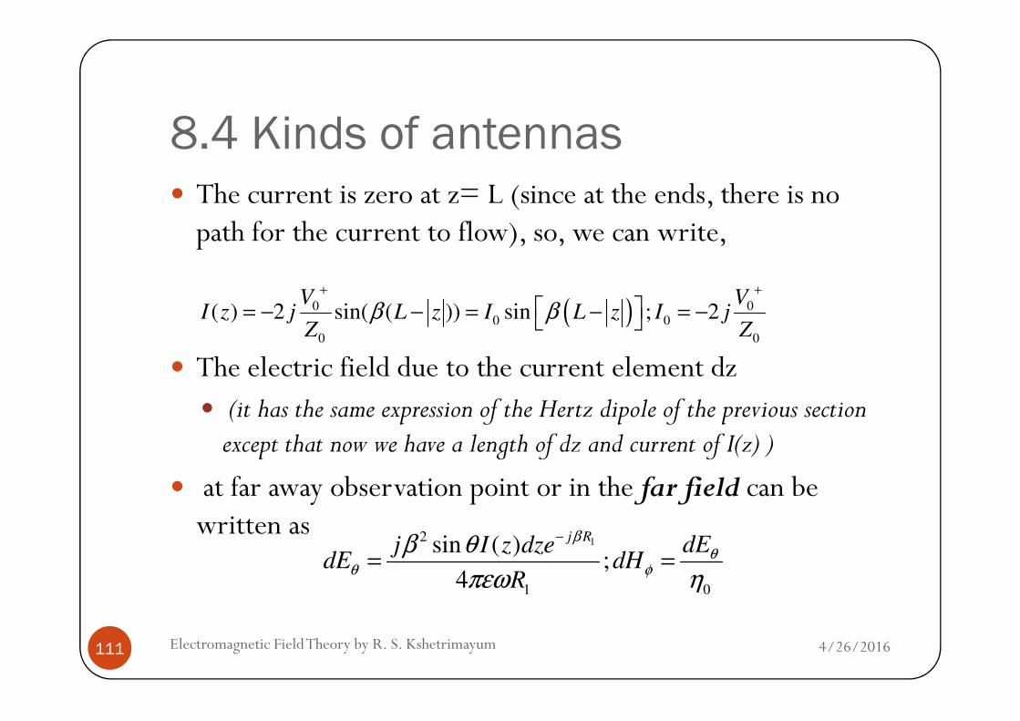
8.4 Kinds of antennas The current is zero at z= L (since at the ends, there is no
path for the current to flow), so, we can write,
The electric field due to the current element dz
( )0 00 0
0 0
( ) 2 sin( ( )) sin ; 2V V
I z j L z I L z I jZ Z
β β+ +
= − − = − = −
4/26/2016Electromagnetic Field Theory by R. S. Kshetrimayum111
The electric field due to the current element dz (it has the same expression of the Hertz dipole of the previous section except that now we have a length of dz and current of I(z) )
at far away observation point or in the far field can be written as
12
1 0
sin ( );
4
j R dEj I z dzedE dH
R
βθ
θ φ
β θ
πεω η
−
= =
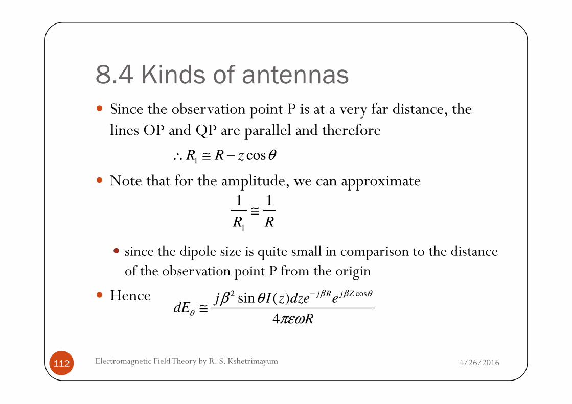
8.4 Kinds of antennas Since the observation point P is at a very far distance, the
lines OP and QP are parallel and therefore
Note that for the amplitude, we can approximate 1 cosR R z θ∴ ≅ −
1 1≅
4/26/2016Electromagnetic Field Theory by R. S. Kshetrimayum112
since the dipole size is quite small in comparison to the distance of the observation point P from the origin
Hence
1
1 1
R R≅
2 cossin ( )
4
j R j Zj I z dze e
dER
β β θ
θ
β θ
πεω
−
≅

8.4 Kinds of antennas Since we have assumed that the dipole of length 2L is
composed of many Hertz dipoles as depicted in Fig. 8.7 (a) (this is one of the reasons why we say that Hertz dipole or
infinitesimal dipole is the building block for many antennas),
we can write the total radiated electric field as
4/26/2016Electromagnetic Field Theory by R. S. Kshetrimayum113
we can write the total radiated electric field as
2 cos2 cos0sin sin( ( ))sin ( )
4 4
j R j ZL L Lj R j Z
z L z L z L
j I L z e ej I z e eE dE dz dz
R R
β β θβ β θ
θ θ
β θ ββ θ
πεω πεω
−−
=− =− =−
−= = =∫ ∫ ∫

8.4 Kinds of antennas It can be shown that (see textbook for derivations)
In the previous equation, the term under bracket is F(θ)
and it is the variation of electric field as a function of θ and
( )( )0 0
cos cos cos60 60
sin
j R j RL Le eE j I j I F
R R
β β
θ
β θ βθ
θ
− − −⇒ ≅ =
4/26/2016Electromagnetic Field Theory by R. S. Kshetrimayum114
and it is the variation of electric field as a function of θ and
it is the E-plane radiation pattern

8.4 Kinds of antennas In the H-plane,
Eθ is a constant and it is not a function of
hence it is a circle
The E–plane radiation pattern of the dipole varies with the length of the dipole as depicted in Fig. 8.8
φ
4/26/2016Electromagnetic Field Theory by R. S. Kshetrimayum115
Note that according to Fig. 8.7 (a), we have considered the total dipole length is 2L) and the H-plane radiation is always a circle
Fig. 8.8 E-plane radiation pattern for dipole of length
(a) 2L=2×λ/4= λ/2
(b) 2L=2×λ=2λ
(c) 2L=2×2λ=4λ

8.4 Kinds of antennas
4/26/2016Electromagnetic Field Theory by R. S. Kshetrimayum116
(a) 2L=2×λ/4= λ/2

8.4 Kinds of antennas
4/26/2016Electromagnetic Field Theory by R. S. Kshetrimayum117
(b) 2L=2×λ=2λ

8.4 Kinds of antennas
4/26/2016Electromagnetic Field Theory by R. S. Kshetrimayum118
(c) 2L=2×2λ=4λ
8.4 Kinds of antennasPoints to be noted:
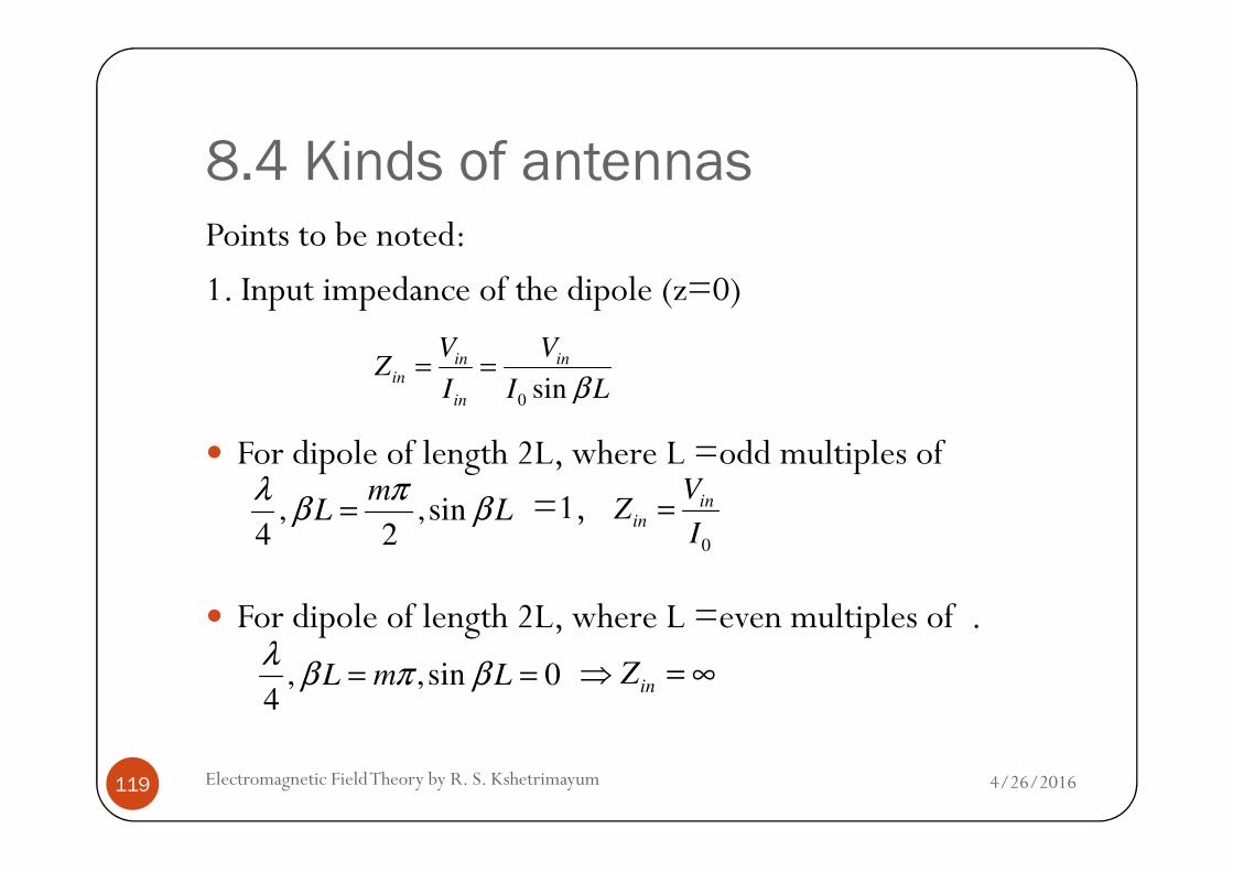
1. Input impedance of the dipole (z=0)
For dipole of length 2L, where L =odd multiples of
0 sin
in inin
in
V VZ
I I Lβ= =
4/26/2016Electromagnetic Field Theory by R. S. Kshetrimayum119
For dipole of length 2L, where L =odd multiples of
=1,
For dipole of length 2L, where L =even multiples of .
, , sin4 2
mL L
λ πβ β=
0
inin
VZ
I=
, , sin 04
L m Lλ
β π β= = inZ⇒ = ∞

8.4 Kinds of antennas That’s why it is preferable to have dipoles of length odd multiples
of λ/2,
otherwise it is difficult to have a source with infinite impedance
2. Since increasing the dipole length more and more current is available for radiation,
4/26/2016Electromagnetic Field Theory by R. S. Kshetrimayum120
available for radiation, • the total power radiated increases monotonically
3. The electric field has only component and hence it is linearly polarized
4. The radiation pattern have nulls and it can be calculated by equating F(θ)=0
$θ

8.4 Kinds of antennas
cos( cos ) cos0
sin
null
null
L Lβ θ β
θ
−=
nullθcos⇒ 1mλ
π= ± ±
4/26/2016Electromagnetic Field Theory by R. S. Kshetrimayum121
o For m=0,
But, in denominator is also zero
So let us take the limit of F(θ) as θ→0, and see
πθ θ ,0cos ,1 =±= nullnull
sinnull
θ

8.4 Kinds of antennas( ) ( ) ( ) ( ) ( ) ( )
0, 0,
2 4 2 4cos cos cos cos cos1
1 1sin sin 2! 4! 2! 4!
L L L L L L
Lim Limθ π θ π
β θ β β θ β θ β β
θ θ→ →
− ≅ − + − − +
( ) ( ) ( ) ( ) ( ) ( )0, 0,
4 42 24 22 1 cos sin 1 cossin sin10
2! 4! sin 2! 4!
L LL L
Lim Limθ π θ π
β θ β θ θβ θ β θ
θ→ →
− + = − × = − =
4/26/2016Electromagnetic Field Theory by R. S. Kshetrimayum122
5. To find θ for maximum radiation, we have to find the solution of
=0
We can also take the mean of the first two nulls to approximate
( )dF
d
θ
θ
maxθ
8.4 Kinds of antennasMonopole antennas:
A monopole is a dipole that has been divided in half at its center feed point and fed against a ground plane
Monopole is usually fed from a coaxial cable (see Fig. 8.7 (b))
4/26/2016Electromagnetic Field Theory by R. S. Kshetrimayum123
Monopole is usually fed from a coaxial cable (see Fig. 8.7 (b))
A monopole of length L placed above a perfectly conducting and infinite ground plane will have the same field distribution to that of a dipole of length
2L without the ground plane

8.4 Kinds of antennas
Monopole
Ground plane
4/26/2016Electromagnetic Field Theory by R. S. Kshetrimayum124
(b) Monopole of length L over a ground plane
Ground plane
Coaxial cable
Dipole in free space
Image of monopole

8.4 Kinds of antennas This is because an image of the monopole will be formed
inside the ground plane (similar to the method of images in chapter 2)
The monopole looks like a dipole in free space (see Fig. 8.7 (b))
4/26/2016Electromagnetic Field Theory by R. S. Kshetrimayum125
(b))
Since this monopole is of length L only, it will radiate only half of the total radiated power of a dipole of
length 2L
Hence, the radiation resistance of a monopole is half that of a dipole

8.4 Kinds of antennas Similarly, directivity of the monopole is twice that of a dipole
Since the field distributions are the same for a monopole and dipole, the maximum radiation intensity will be also same for both
cases
4/26/2016Electromagnetic Field Theory by R. S. Kshetrimayum126
cases
But for monopole, the total radiated power is half that of a dipole
Hence, the directivity of a monopole above a conducting ground plane is twice that of dipole in free space
8.4 Kinds of antennas8.4.3 Loop antenna
Loop antennas could be of various shapes: circular,
triangular,
square,
4/26/2016Electromagnetic Field Theory by R. S. Kshetrimayum127
square,
elliptical, etc.
They are widely used in applications up to 3GHz
Loop antennas can be classified into two: electrically small (circumference < 0.1 λ) and
electrically large (circumference approximately equals to λ)

8.4 Kinds of antennas Electrically small loop antennas have
very small radiation resistance
They have very low radiation and
are practically useless
4/26/2016Electromagnetic Field Theory by R. S. Kshetrimayum128
are practically useless
Electrically small loop antennas could be analyzed assuming that it is equivalently represented as a Hertz dipole
Let us consider electrically large circular loop of constant current

8.4 Kinds of antennas Fig. 8.9 Loop antenna
θrr
4/26/2016Electromagnetic Field Theory by R. S. Kshetrimayum129
φ
'φ
'P
'rr
ψ
Rr

8.4 Kinds of antennas We can express magnetic vector potential (see textbook) as
( )( )
( )
01 1
2
1 120
( ) ( sin ) ( sin )4
1( ) ( 1) ( ) ( sin ) ( sin )
2 ! !
j r
m m
n n
n n nm nm
I aeA j J a J a
r
zJ z z J z J z J a J a
m n m
β
φ
µθ π β θ β θ
π
β θ β θ
−
∞
+=
= − −
−= ∴ − = − ⇒ − = −
+∑Q
4/26/2016Electromagnetic Field Theory by R. S. Kshetrimayum130
We can express electric field as
( )0
0 1
2 ! !
( sin )( )
2
m
j r
m n m
j I ae J aA
r
β
φ
µ β θθ
=
−
+
∴ =
( )AE j j Aω
ωµε
∇ ∇ •∴ = − −
rrr

8.4 Kinds of antennas Note that magnetic vector potential has only component
which is a function of θ variable onlyφ
0 1
0;
( sin )0 0; 0
j r
r r r
A
I ae J aA A E j A E j A E j A
β
θ θ θ φ φ
ωµ β θω ω ω
−
∴∇ • =
= = ⇒ = − = = − = ∴ = − =
r
Q
4/26/2016Electromagnetic Field Theory by R. S. Kshetrimayum131
0 0; 02
r r rA A E j A E j A E j A
rθ θ θ φ φω ω ω= = ⇒ = − = = − = ∴ = − =Q
( )01 sin ; 0
2
j r
r
E I aeH J a H H
r
βφ
θ φ
ωµβ θ
η η
−−= − = = =

8.4 Kinds of antennas Poynting vector for a wave radiating in radially outward
direction should have direction along positive radial direction
Therefore must be negative Fig. 8.10 shows the far-field radiation pattern of the loop
Hθ
4/26/2016Electromagnetic Field Theory by R. S. Kshetrimayum132
Fig. 8.10 shows the far-field radiation pattern of the loop antenna
It can be observed that the radiation field has higher magnitude with the larger radius of the loop antenna
For larger radiation power we need a loop antenna of larger radius

8.4 Kinds of antennas
4/26/2016Electromagnetic Field Theory by R. S. Kshetrimayum133
Fig. 8.10 Plot of for various values of angle θ (far-field radiation patterns) (dotted line a=0.1λ, dashed line a=0.2λ, solid line a=0.3λ)

8.4 Kinds of antennas For small loops
( ) θβθβθβθββ sin2
1...sin
16
1sin
2
1)sin(;
3
1 31 aaaaJa ≅+−=<
( ) ( )0 01 1sin ; sin
j r j rI a I ae eE a H a
β β
φ θ
ωµ ωµβ θ β θ
η
− −
∴ = = −
4/26/2016Electromagnetic Field Theory by R. S. Kshetrimayum134
Note that for the dipole polarization was along direction
But for small loop antennas it is along the direction
( ) ( )sin ; sin2 2 2 2
E a H ar r
φ θβ θ β θη
∴ = = −
θ
φ

8.5 Antenna Arrays
One of the disadvantages of single antenna is that it has fixed radiation pattern
That means once we have designed and constructed an antenna, the beam or radiation pattern is fixed
4/26/2016Electromagnetic Field Theory by R. S. Kshetrimayum135
the beam or radiation pattern is fixed
If we want to tune the radiation pattern, we need to apply the technique of antenna arrays
Antenna array is a configuration of multiple antennas (elements) arranged
to achieve a given radiation pattern

8.5 Antenna Arrays
There are several array design variables which can be changed to achieve the overall array pattern design
Some of the array design variables are:
(a) array shape linear, circular,
4/26/2016Electromagnetic Field Theory by R. S. Kshetrimayum136
circular, planar, etc.
(b) element spacing
(c) element excitation amplitude
(d) element excitation phase
(e) patterns of array elements
φ

8.5 Antenna Arrays
Given an antenna array of identical elements, the radiation pattern of the antenna array may be found
according to the pattern multiplication principle
It basically means that array pattern is equal to φ
4/26/2016Electromagnetic Field Theory by R. S. Kshetrimayum137
It basically means that array pattern is equal to the product of the
pattern of the individual array element into
array factor , a function dependent only on
the geometry of the array
the excitation amplitude and phase of the elements
φ

8.5 Antenna Arrays
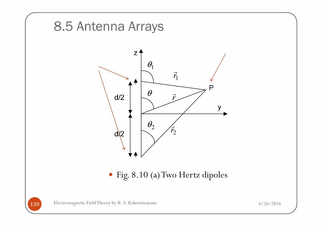
8.5.1 Two element array
Let us investigate an array of two infinitesimal dipoles positioned along the z axis as shown in Fig.
8.10 (a)
The field radiated by the two elements, assuming no coupling between the elements
4/26/2016Electromagnetic Field Theory by R. S. Kshetrimayum138
assuming no coupling between the elements
is equal to the sum of the two fields
where the two antennas are excited with current
1 1 2 22 2
1 21 2
1 2
sin sinˆ ˆ4 4
j r j j r j
total
jI dl e e jI dl e eE E E
r r
β δ β δθ β θ βθ θ
πεω πεω
− −
= + = +r r r
1 1 2 2I and Iδ δ< <
8.5 Antenna Arrays
1rr
rr
1θ
θ
4/26/2016Electromagnetic Field Theory by R. S. Kshetrimayum139
Fig. 8.10 (a) Two Hertz dipoles
2rr2θ

8.5 Antenna Arrays
For 1 2 oI I I= =
1 2,2 2
α αδ δ= = −
2 cos cossinˆd dj r j jjI dl e
β α β αβ θ θθβθ
− + − + = +
r
4/26/2016Electromagnetic Field Theory by R. S. Kshetrimayum140
2 cos cos2 2 2 20 sinˆ
4
j r j j
total
jI dl eE e e
r
β θ θθβθ
πεω
− + − +
= +
r
2
0 sinˆ 2cos cos4 2 2
j rjI dl e d
r
βθβ β αθ θ
πεω
− = +

8.5 Antenna Arrays
Hence the total field of the array is equal to
the field of single element positioned at the origin
multiplied by a factor which is called as the array factor
Array factor is given
4/26/2016Electromagnetic Field Theory by R. S. Kshetrimayum141
Normalized array factor is
( )1
2cos cos2
AF dβ θ α
= +
( )2
1cos cos
2AF dβ θ α
= +

8.5 Antenna Arrays
8.5.2 N element uniform linear array (ULA) This idea of two element array can be extended
to N element array of uniform amplitude and spacing
Let us assume that N Hertz dipoles are placed along a straight line along z-axis at positions
4/26/2016Electromagnetic Field Theory by R. S. Kshetrimayum142
straight line along z-axis at positions 0, d, 2d, …, (N-2) d and (N-1) d respectively

8.5 Antenna Arrays Current of equal amplitudes
but with phase difference of 0, α, 2α, … , (N-2) α and (N-1) α
4/26/2016Electromagnetic Field Theory by R. S. Kshetrimayum143
are excited to the corresponding dipoles at 0, d, 2d, …, (N-2) d and (N-1) d respectively

8.5 Antenna Arraysz
2d
(N-1)d
.
.
.
2I α⟨
( 1)I N α⟨ −
0I ⟨
I α⟨
( 1)
2
NI α
−⟨
4/26/2016Electromagnetic Field Theory by R. S. Kshetrimayum144
Fig. 8.10 (b) ULA 1 (c) ULA 2 (assume N is an odd number)
d
2d
00I ⟨
I α⟨
2I α⟨0I ⟨
I α⟨−
( 1)
2
NI α
−⟨−

8.5 Antenna Arrays
Then the array factor for the N element ULA of Fig. 8.10 (b) will become
( ) ( ) ( )cos 2 cos ( 1) cos1 .....
j d j d j N dAF e e e
β θ α β θ α β θ α+ + − +∴ = + + + +
( )( )ψ−1 e
jNN
4/26/2016Electromagnetic Field Theory by R. S. Kshetrimayum145
( )( ) αθβψψ
ψαθβ +=
−
−=⇒=⇒ ∑
=
+− cos;1
1
1
cos1d
e
eAFeAF
j
jN
N
N
n
dnj
1
1
jN
j
e
e
ψ
ψ−
=−
( ) ( )1 2 2( )2
1 1( ) ( )2 2
N Nj jN
j
j j
e ee
e e
ψ ψψ
ψ ψ
−−
−
−=
−
1( )
2
sin( )2
sin( )2
Nj
N
eψ
ψ
ψ
−
=

8.5 Antenna Arrays
If the reference point is at the physical
center of the array as depicted in
Fig. 8.10 (c), the array factor is
( )sin( )
2
Nψ
0I ⟨
I α⟨
( 1)
2
NI α
−⟨
4/26/2016Electromagnetic Field Theory by R. S. Kshetrimayum146
For small values of
( )sin( )
2
sin( )2
NAF
ψ
ψ=
( )sin( )
2
2
N
N
AF
ψ
ψ=
0I ⟨
I α⟨−
( 1)
2
NI α
−⟨−

8.5 Antenna Arrays
The maximum value of AF is for and its value is N
Apply L’ Hospital rule since it is of the form
To normalize the array factor so that the maximum value is equal to unity, we get,
0ψ =
0
0sin
4/26/2016Electromagnetic Field Theory by R. S. Kshetrimayum147
( )sin( )
1 21
sin2
N
N
AFN
ψ
ψ
=
sin( )2
2
N
N
ψ
ψ≅

8.5 Antenna Arrays
This is the normalized array factor for ULA As N increases, the main lobe narrows The number of lobes is equal to N
one main lobe and other N-1 side lobes
4/26/2016Electromagnetic Field Theory by R. S. Kshetrimayum148
other N-1 side lobes
in one period of the AF The side lobes widths are of 2/N and main lobes are two times wider than the side lobes The SLL decreases with increasing N This can be verified from Fig. 8.11 (see textbook)
8.5 Antenna Arrays
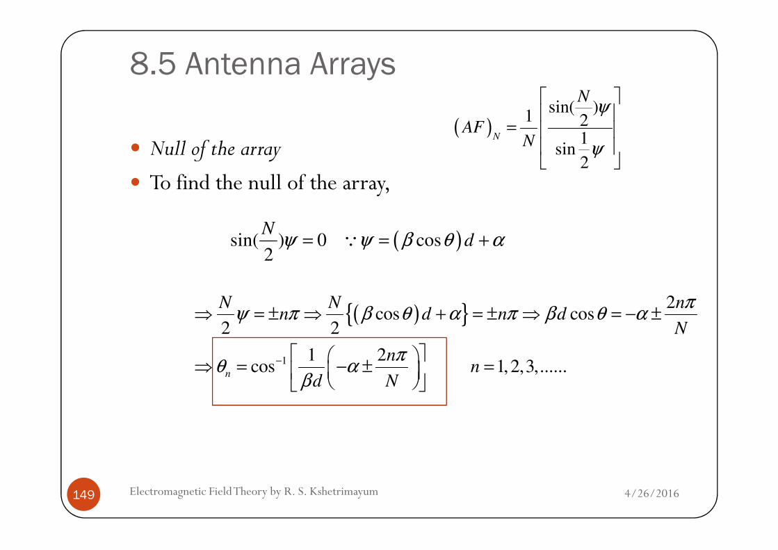
Null of the array
To find the null of the array,
( )sin( ) 0 cos2
Ndψ ψ β θ α= = +Q
( )sin( )
1 21
sin2
N
N
AFN
ψ
ψ
=
4/26/2016Electromagnetic Field Theory by R. S. Kshetrimayum149
( )
1
2cos cos
2 2
1 2cos 1,2,3,......
n
N N nn d n d
N
nn
d N
πψ π β θ α π β θ α
πθ α
β−
⇒ = ± ⇒ + = ± ⇒ = − ±
⇒ = − ± =

8.5 Antenna Arrays
Maximum values
It attains the maximum values for 0ψ =
( )1
cos2 2
m
dθ θ
ψβ θ α
=
= + 0=
( )sin( )
1 21
sin2
N
N
AFN
ψ
ψ
=
4/26/2016Electromagnetic Field Theory by R. S. Kshetrimayum150
8.5.3 Broadside array
We know that when
mθ θ=
1cosmd
αθ
β−
−
⇒ =

8.5 Antenna Arrays
the maximum radiation occurs
It is desired that maximum occurs at θ=90˚
c o s 0dψ β θ α= + =
0
0
90cos 0 0d
θψ β θ α α
== + = ⇒ =
4/26/2016Electromagnetic Field Theory by R. S. Kshetrimayum151
8.5.4 Endfire array
We know that when
the maximum radiation occurs
090cos 0 0d
θψ β θ α α
== + = ⇒ =
cos 0dψ β θ α= + =
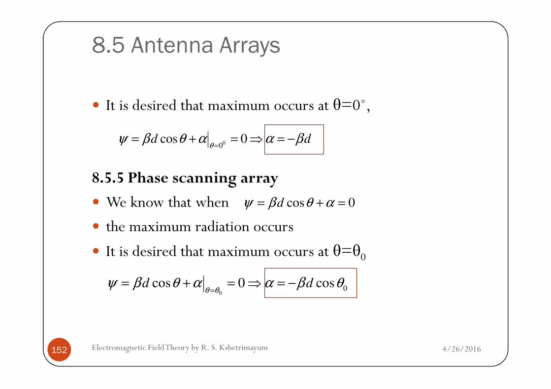
8.5 Antenna Arrays
It is desired that maximum occurs at θ=0˚,
8.5.5 Phase scanning array
We know that when
00cos 0d d
θψ β θ α α β
== + = ⇒ = −
4/26/2016Electromagnetic Field Theory by R. S. Kshetrimayum152
We know that when
the maximum radiation occurs
It is desired that maximum occurs at θ=θ0
cos 0dψ β θ α= + =
00cos 0 cosd d
θ θψ β θ α α β θ
== + = ⇒ = −

8.5 Antenna Arrays
Draw the polar plot of radiation pattern for the following
uniform linear array (ULA)
of N isotropic radiating antennas spaced λ/2
apart for the following cases: θ
I α⟨
( 1)
2
NI α
−⟨
4/26/2016Electromagnetic Field Theory by R. S. Kshetrimayum153
(a) Broadside array (Maximum field is at θ=90˚)
(b) End fire array (Maximum field is at θ=0˚)
(c) Maximum field is at θ=60˚ and
(d) Null at θ=60˚
( )sin( )
1 21
sin2
N
N
AFN
ψ
ψ
=
0I ⟨
I α⟨−
( 1)
2
NI α
−⟨−

8.5 Antenna Arrays 0
0
90cos 0 0d
θψ β θ α α
== + = ⇒ =
4/26/2016Electromagnetic Field Theory by R. S. Kshetrimayum154
(a) Broadside array (Maximum field is at θ=90˚)
8.5 Antenna Arrays 00cos 0d d
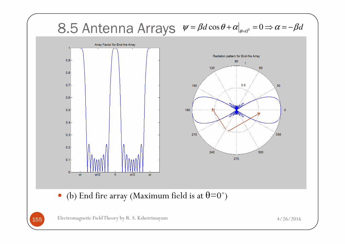
θψ β θ α α β
== + = ⇒ = −
4/26/2016Electromagnetic Field Theory by R. S. Kshetrimayum155
(b) End fire array (Maximum field is at θ=0˚)
8.5 Antenna Arrays
4/26/2016Electromagnetic Field Theory by R. S. Kshetrimayum156
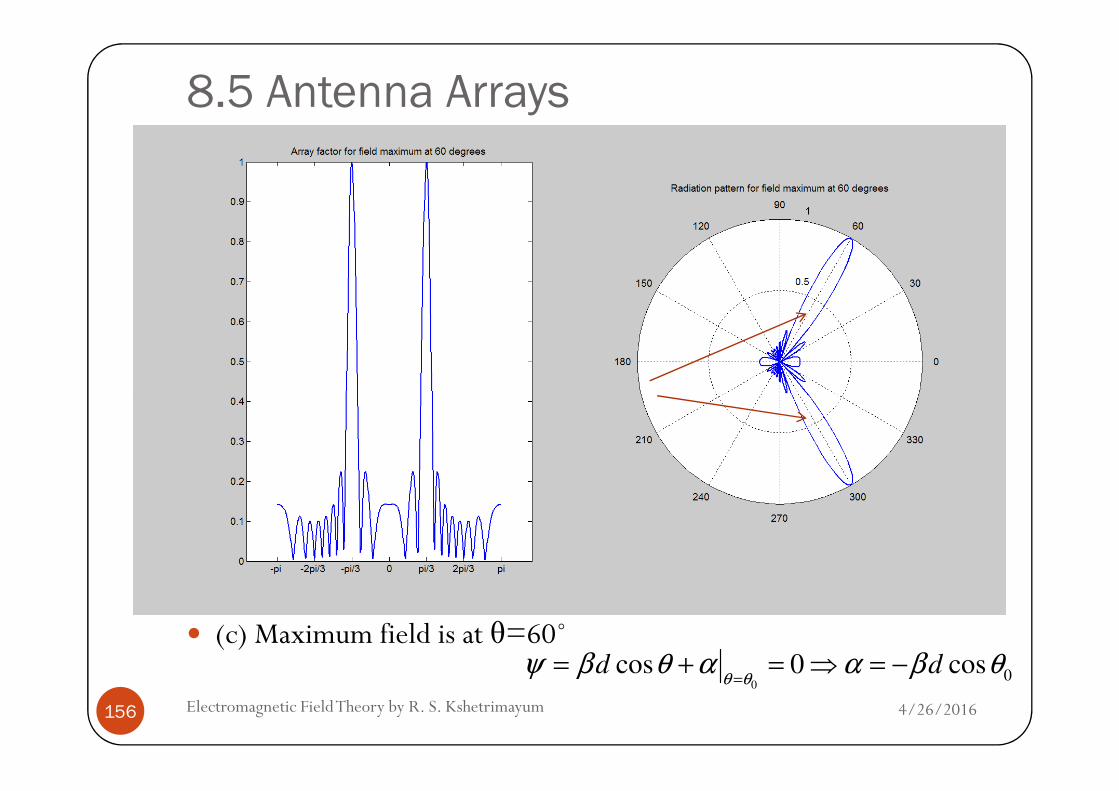
(c) Maximum field is at θ=60˚
00cos 0 cosd d
θ θψ β θ α α β θ
== + = ⇒ = −

8.5 Antenna Arrays
4/26/2016Electromagnetic Field Theory by R. S. Kshetrimayum157
(d) Null at θ=60˚L,3,2,1,cos
2=−= nd
N
nnullθβ
πα