Symmetry, Integrability and Geometry: Methods and Applications SIGMA 8 (2012), 022, 20 pages

Conformally Equivariant Quantization –

a Complete Classif ication

Jean-Philippe MICHEL

University of Luxembourg, Campus Kirchberg, Mathematics Research Unit,6, rue Richard Coudenhove-Kalergi, L-1359 Luxembourg City, LuxembourgE-mail: jean-philippe.michel@uni.luURL: http://math.uni.lu/~michel/SitePerso/indexLux.html

Received July 29, 2011, in final form April 11, 2012; Published online April 15, 2012

http://dx.doi.org/10.3842/SIGMA.2012.022

Abstract. Conformally equivariant quantization is a peculiar map between symbols ofreal weight δ and differential operators acting on tensor densities, whose real weights aredesigned by λ and λ + δ. The existence and uniqueness of such a map has been provedby Duval, Lecomte and Ovsienko for a generic weight δ. Later, Silhan has determined thecritical values of δ for which unique existence is lost, and conjectured that for those valuesof δ existence is lost for a generic weight λ. We fully determine the cases of existence anduniqueness of the conformally equivariant quantization in terms of the values of δ and λ.Namely, (i) unique existence is lost if and only if there is a nontrivial conformally invariantdifferential operator on the space of symbols of weight δ, and (ii) in that case the conformallyequivariant quantization exists only for a finite number of λ, corresponding to nontrivialconformally invariant differential operators on λ-densities. The assertion (i) is proved in themore general context of IFFT (or AHS) equivariant quantization.

Key words: quantization; (bi-)differential operators; conformal invariance; Lie algebra co-homology

2010 Mathematics Subject Classification: 53A55; 53A30; 17B56; 47E05

1 Introduction

Quantization originates from physics, and lies at the correspondence between classical and quan-tum formalisms. It has given the impetus for the development of numerous mathematical theo-ries, and admits as many different definitions. In this paper, by quantization we mean theinverse of a certain symbol map, i.e. a linear map from functions on a cotangent bundle T ∗M ,which are polynomial in the fiber variables, to the space of differential operators on M . Nosuch quantization can be canonically defined from the differential geometry of M . The ideaof equivariant quantization is to build one from a richer geometric structure on M : the localaction of a Lie group G, or equivalently, of its Lie algebra g. This imposes the condition thatthe manifold M possesses a locally flat G-structure.

Equivariant quantization was first developed for projective and conformal structures by Du-val, Lecomte and Ovsienko [7, 17]. There, the condition of equivariance singles out a uniquequantization up to normalization. Generalizations to the curved case have been proposed re-cently in terms of Cartan connections [19, 20] or tractors [6, 23], but we restrict ourselves here tothe locally flat case, or equivalently to Rn. In [4], Boniver and Mathonet exhibit the correct classof Lie algebras to be considered for equivariant quantization. It is provided by maximal Lie sub-algebras g among those of finite dimension in Vectpol(Rn), the Lie algebra of polynomial vectorfields. They prove in [5] that these Lie algebras are precisely the irreducible filtered Lie algebrasof finite type (with no complex structure) classified by Kobayashi and Nagano [13], referred to asIFFT-algebras. Particular examples are the Lie algebra sln+1 ' sl(n+ 1,R) of projective vector

arX

iv:1

102.

4065

v3 [

mat

h.D

G]

15

Apr

201

2

2 J.-P. Michel

fields, and the Lie algebra cf ' o(p+1, q+1) of conformal Killing vector fields on (Rn, η), wheren = p + q and η is the flat metric of signature (p, q). Generalizing [4], Cap and Silhan provein [6] the existence and uniqueness of the g-equivariant quantization with values in differentialoperators acting on irreducible homogeneous bundles, barring certain exceptional bundles. Thedetermination of these exceptional cases and their geometric interpretation is an open problem,since they appear in the seminal work [7] dealing with bundles of tensor densities |ΛnT ∗Rn|⊗λof arbitrary weight λ ∈ R. Our paper is devoted to a step towards its solution. We give a com-plete resolution in the original case of conformally equivariant quantization Qλ,µ : Sδ → Dλ,µwith values in the space Dλ,µ of differential operators from λ- to µ-tensor densities, the symbolsbeing here of weight δ = µ− λ.

This work can be regarded in the broader perspective of invariant bidifferential operators,whose equivariant quantization is an example. Another example is provided by generalizedtransvectants (or Rankin–Cohen bracket), whose arguments are spaces of weighted densities.There the same phenomenon occurs: they exist and are unique except for certain exceptionalweights [22]. In fact, this is general, as proved by Kroeske in his thesis [14], where he stu-dies invariant bidifferential operators for parabolic geometries. From a number of examplesand a proof in the projective case [15], Kroeske proposes a paradigm which can be roughlyphrased as follows: every exceptional case of existence or uniqueness of an invariant bidifferentialoperator originates from the existence of a nontrivial invariant differential operator on one ofthe factors. We show that this is particularly illuminating in the case of equivariant quan-tization. Namely, resorting to the interpretation in terms of cohomology of g-modules deve-loped by Lecomte in [16], we prove our first main result: unique existence of g-equivariantquantization is lost if and only if there exists a g-invariant operator on the space of sym-bols. Remarkably, this correspondence is proved directly rather than obtained a posteriori,like in the work of Kroeske. The theory of invariant operators being well-developed, we getan efficient way to determine the exceptional bundles for equivariant quantization. Retur-ning to the aforementioned conformally equivariant quantization Qλ,µ : Sδ → Dλ,µ, we recoverthe set of critical values of δ for which unique existence is lost, already determined by Sil-han [23].

The next natural question is to determine for which resonant pairs of irreducible homoge-neous bundles the g-equivariant quantization exists but is not unique. This turns to be anharder question, and we address it only for pairs of line bundles of tensor densities. By ourfirst main theorem, we can obtain the critical shift δ = µ − λ of their weights for which thereis not existence and uniqueness of the g-equivariant quantization. We have then to determinethe resonant values (λ, µ) for which the g-equivariant quantization still exists. In the projec-tive case, an explicit formula for the quantization provides the answer [9, 17]. Moreover, thesituation has been fully understood in terms of cohomology of sln+1-modules, the existence ofthe projectively equivariant quantization being characterized by the triviality of a 1-cocycle,which depends on δ and λ [16]. Using a similar approach, we obtain our second main result: foreach critical value δ of the conformally equivariant quantization Qλ,µ, there is a finite numberof resonances (λ, λ + δ) that we determine. This completes the known results on symbols ofdegree at most 3, and proves a conjecture of Silhan: the conformally equivariant quantizationdoes generically not exist for δ critical. In addition, we provide an interpretation along thelines of the Kroeske’s paradigm: the resonances correspond to conformally invariant operatorson the source space of densities, e.g. the conformal powers of the Laplacian. This allows us toconstruct conformally equivariant quantization in the resonant cases. Together with Silhan’swork [23], this provides construction for the conformally equivariant quantization whenever itexists.

Let us outline the contents of this paper. Section 2 is devoted to the proof of Theo-rem 2.5: for g an IFFT-algebra, the g-equivariant quantization exists and is unique if and

Conformally Equivariant Quantization – a Complete Classification 3

only if there is no g-invariant differential operator on the space of symbols which strictly lo-wers the degree. It relies on the fact that equivariant quantization exists if a certain 1-cocycleis a coboundary. We know from [4] that this is the case for generic δ′, and this property isstable in the limit δ′ → δ if the space of 1-coboundaries is of constant dimension. That con-dition happens to be equivalent to the absence of g-invariant operators on δ-weighted sym-bols. In Sections 3 and 4 we illustrate and complete Theorem 2.5 for, respectively, g theprojective and the conformal Lie algebras, the quantization being valued in differential ope-rators acting on tensor densities. First, we determine the critical values via the classificationof invariant operators on the space of symbols. Then we prove that those invariant opera-tors give rise to nontrivial 1-cocycles. They obstruct existence of the equivariant quantizationexcept when there is an invariant differential operator from λ-densities to a certain homoge-neous bundle. Finally, the latter operator allows us to construct an equivariant quantization,proving thus its existence for exactly those values of λ. That leads to the complete list ofresonances (λ, λ + δ), together with their interpretation in terms of invariant operators on thespace of λ-densities. We end Section 4 with a detailed treatment of the symbols of degree lessthan 3, thus interpreting the results of Loubon Djounga [18] along the line of the Kroeske’sparadigm. The last section gives us the opportunity to propose some natural extensions of ourresults.

Throughout this paper, the space of linear maps between two real vector spaces V and W isdenoted by Hom(V,W ), and its elements are called operators. We work on Rn and the Einsteinsummation convention is understood.

2 On the existence and uniqueness of equivariant quantization

2.1 Definition of equivariant quantization

We start with the definitions of the algebra D(Rn) of differential operators on Rn, and its algebraof symbols S(Rn). The former is filtered by the subspaces Dk(Rn) of differential operators oforder k, defined as the spaces of operators A on C∞(Rn) satisfying [. . . [A, f0], . . . ], fk] = 0 for allfunctions f0, . . . , fk ∈ C∞(Rn), considered here as (zero order) operators on C∞(Rn). The latteris the canonically associated graded algebra, defined by S(Rn) =

⊕∞k=0Dk(Rn)/Dk−1(Rn). This

may be identified with the algebra of functions on T ∗Rn that are polynomial in the fibers, thegrading corresponding to the polynomial degree. The canonical projection σk : Dk(Rn) →Dk(Rn)/Dk−1(Rn) is called the principal symbol map. It admits a section, the normal ordering,given by

N : P i1...ik(x)pi1 · · · pik 7→ P i1...ik(x)∂i1 · · · ∂ik , (2.1)

where (xi, pi) are coordinates on T ∗Rn. This defines a linear isomorphism S(Rn) ' D(Rn).

We are interested in the action of vector fields on these both algebras. First of all, we intro-duce the Vect(Rn)-module of λ-densities Fλ = (C∞(Rn), `λ) as a one parameter deformation ofthe module C∞(Rn), the Vect(Rn)-action being given by X 7→ `λX = X + λDiv(X), with Divthe divergence and λ ∈ R the weight of the densities. This module corresponds geometrically tothe space of sections of the trivial line bundle |ΛnT ∗Rn|⊗λ. It gives rise to the Vect(Rn)-moduleDλ,µ = (D(Rn),Lλ,µ) of differential operators from λ- to µ-densities, endowed with the adjointaction

Lλ,µX A = `µXA−A`λX ,

for all X ∈ Vect(Rn) and A ∈ D(Rn). This action preserves the filtration of D(Rn), and sothe algebra of symbols inherits a Vect(Rn)-module structure compatible with the grading. We

4 J.-P. Michel

denote this structure by Sδ = (S(Rn), Lδ), where δ = µ− λ is the shift. The action of Vect(Rn)is given in coordinates by

LδX = Xi∂i − pj(∂iXj)∂pi + δDiv(X), (2.2)

and coincides with the canonical action on functions on T ∗M tensored with δ-densities. Wedenote by Sδk the submodule of homogeneous symbols of degree k.

Definition 2.1. Let g be a Lie subalgebra of Vect(Rn). A g-equivariant quantization is a g-module morphism

Qλ,µ : Sδ → Dλ,µ,

such that Qλ,µ is a right inverse of the principal symbol map on homogeneous symbols.

Using the normal ordering (2.1), we freely identify Dλ,µ with (S(Rn),Lλ,µ), where we keep thesame notation for Lλ,µ and its pull-back on symbols by N . It is then a matter of computationto prove that Lλ,µX = LδX if X is an affine vector field and δ = µ − λ. In other words, N is anaff(n,R)-equivariant quantization [7].

2.2 IFFT-algebras and equivariant quantization

An IFFT-algebra g is a simple Lie subalgebra of the polynomial vector fields on Rn. Assuch, it admits a gradation by the degree of the vector field components g = g−1 ⊕ g0 ⊕ g1

which is compatible with the bracket: [gi, gj ] = gi+j , where gi = {0} if i /∈ {−1, 0, 1}. TheLie subalgebra g−1 consists of translations, g1 consists of so-called g-inversions, and g0 con-tains the dilation and acts irreducibly on both g−1 and g1. Consequently, g-invariance isequivalent to g−1 ⊕ g0-invariance plus the invariance with respect to one non-zero elementin g1.

Let us introduce some notation. For h a Lie subalgebra of Vect(Rn), the space of h-invariantoperators between two h-submodules F ⊂ Sδ and F ′ ⊂ Sδ′ is defined as

Homh(F, F′) = {A ∈ Hom(F, F ′) | ∀X ∈ h, [L∗X , A] = 0}, (2.3)

where the commutator [L∗X , A] is a symbolic notation for Lδ′XA − ALδX . Note that the vector

fields which preserve F and F ′ clearly act on Homh(F, F′). We define similarly the space of

h-invariant differential operators Dh(F, F′) and its module structure.

Lemma 2.2 ([17]). Let g be an IFFT-algebra, and fix l < k. The vector space Homg−1⊕g0(Sδk ,Sδl )is finite-dimensional, independent of δ, and equal to the space Dg−1⊕g0(Sδk ,Sδl ) of invariantdifferential operators.

Proof. We only need the fact that g−1⊕ g0 contains the translations and the dilation. Indeed,an operator A ∈ Hom(Sδk ,Sδl ) invariant with respect to those transformations was proved in [17]to be a differential operator if l < k. Hence it is generated by the coordinates pi and thederivatives ∂i, ∂pi . Now the dilation invariance ensures that the degree in ∂i is equal to the degreein ∂pi minus the degree in pi. The degree in ∂pi being k at most, the space Homg−1⊕g0(Sδk ,Sδl )is finite-dimensional. Since the divergence of affine vector fields is a constant, the action ofg−1 ⊕ g0 on Hom(Sδk ,Sδl ) is independent of δ and hence the subspace of g−1 ⊕ g0-invariantoperators is also. �

Conformally Equivariant Quantization – a Complete Classification 5

We turn now to the study of the g-equivariance condition for a quantization Qλ,µ. We canalways factor the latter through the normal ordering, defining the linear automorphism Qλ,µ

of Sδ by Qλ,µ = N ◦Qλ,µ. Restricting to Sδk , we then get

Qλ,µ =

k∑l=0

φl, (2.4)

where φ0 = Id and φl ∈ Hom(Sδk ,Sδk−l). Since the normal ordering is aff(n,R)-equivariant, we

deduce from Lemma 2.2 that more precisely φl ∈ Dg−1⊕g0(Sδk ,Sδk−l) for all l = 1, . . . , k. The full

equivariance condition for Qλ,µ reads then on Sδk as[φl, L

δX

]=(Lλ,µX − LδX

)φl−1, (2.5)

for all l = 1, . . . , k, where X is a non-zero element of g1. To solve it directly is too intricateexcept for g = sln+1. Nevertheless, the following theorem has been proven in [4], resorting tosimultaneous diagonalization of the Casimir operators on the modules of symbols and differentialoperators. We also refer to [6], where the additional hypothesis of simplicity of the semi-simplepart of g0 is dropped.

Theorem 2.3 ([4, 6]). Let g be an IFFT-algebra and fix k ∈ N. The g-equivariant quantization

Qλ,µ : Sδk → Dλ,µk exists and is unique if µ− λ = δ /∈ Ik, with Ik a finite subset of Q.

2.3 Equivariant quantization and Lie algebra cohomology

We give here a cohomological interpretation of the equations (2.5) encoding the equivarianceof Qλ,µ. Let us first give a brief review of the cohomology of g-modules and its link with thesplitting of exact sequences of g-modules (see [12] for more details). The cohomology of theg-module (M,LM ) is defined in terms of the k-cochains, which are the linear maps Λkg → M ,and the differential d which reads, on 0- and 1-cochains φ and γ,

dφ(X) = LMX φ, dγ(X,Y ) = LMX γ(Y )− LMY γ(X)− γ([X,Y ]), (2.6)

where X, Y are in g. Let now (A,LA), (B,LB), (C,LC) be three g-modules, and suppose thatwe have an exact sequence of g-modules,

0 // (A,LA)ι // (B,LB)

σ // (C,LC)

τii

// 0,

with τ a linear section. This defines a 1-cocycle γ = ι−1(LB ◦ τ − τ ◦ LC) with values inHom(C,A). Its cohomolgical class does not depend on the choice of linear section τ , and thesequence of g-modules is split if and only if γ = dφ is a coboundary. The splitting morphism isthen τ + ι ◦ φ. Moreover, if γ vanishes on a Lie subalgebra h then φ is h-invariant.

The existence and uniqueness of a g-equivariant quantization can be rephrased in terms ofcohomology of g-modules [16]. Indeed, such a quantization exists if for every k ∈ N the exactsequence

0→ Dλ,µk−1 → Dλ,µk → Sδk → 0

is split in the category of g-modules. Using the normal ordering as a linear splitting, thismeans that the 1-cocycle γ = Lλ,µ − Lδ admits a trivial cohomology class [γ]. By vanishingof γ on the affine part of g, the latter pertains to the following relative cohomology spaceH1(g, g−1⊕ g0; Hom(Sδk ,D

λ,µk−1)). The modules Hom(Sδk ,D

λ,µk−1) are quite complex to handle, but

6 J.-P. Michel

modding out by Dλ,µk−l for increasing l, we are reduced by induction to the simpler modules

Hom(Sδk ,Sδk−l). Thus, a g-equivariant quantization on F δ, a submodule of Sδk , is a section of

g-modules ψk : F δ → Dλ,µk defined inductively by ψ0 = Id and the commutative triangle in thefollowing diagram of g-modules

0 // Sδk−l // Dλ,µk /Dλ,µk−l−1// Dλ,µk /Dλ,µk−l // 0

F δ?�

ψl−1

OO

T4

∃?ψl

gg(2.7)

for successively all l = 1, . . . , k. With notation as in (2.4), we have ψl =∑l

i=0 φi. In the nextlemma we recover the equivariance condition (2.5) using this cohomological approach.

Lemma 2.4. The partial quantization ψl defined in (2.7) exists if and only if ψl−1 exists andthe 1-cocycle γl = (Lλ,µ − Lδ)φl−1, whose class belongs to H1(g, g−1 ⊕ g0; Hom(F δ,Sδk−l)), istrivial. In this case, we have ψl = ψl−1 + φl, where φl satisfies[

φl, LδX

]= γl(X) (2.8)

for some non-zero X in g1 and φl ∈ Dg−1⊕g0(F δ,Sδk−l).

Proof. Via the normal ordering, ψl−1 lifts linearly to Dλ,µk /Dλ,µk−l−1. The existence of the mor-

phism ψl relies then on the triviality of the 1-cocycle (Lλ,µ−Lδ)ψl−1. As it takes values in Sδk−l,and as Lλ,µX −LδX lowers the degree by one, the previous 1-cocycle is equal to γl. Thus ψl existsif and only if γl = dφl, and ψl = ψl−1 + φl is the splitting morphism. From the definition of γl,we get the g−1⊕ g0-invariance of φl. Finally, the irreducibility of the action of g0 on g1 togetherwith definition of 1-cocycles shows that (2.8) is equivalent to the triviality of γl. �

2.4 Main result

We can now give a characterization of the critical values δ of the g-equivariant quantization interms of g-invariant operators.

Theorem 2.5. Let g be an IFFT-algebra and let F δ = (F,Lδ) be a g-submodule of Sδk forevery δ ∈ R. The g-equivariant quantization exists and is unique on F δ if and only if thereexists no non-zero g-invariant differential operator from F δ to Sδk−l, for l = 1, . . . , k.

Proof. Let δ ∈ Ik, defined in Theorem 2.3. Clearly, if there exists a g-equivariant quantizationon F δ, its uniqueness is equivalent to the absence of g-invariant operator from F δ to Sδk−l forl = 1, . . . , k. We only have to prove that such an absence implies existence of the g-equivariantquantization on F δ. By induction on l, this amounts to obtaining the partial quantization ψlout of ψl−1. By the preceding lemma, this means to prove that the 1-cocycle γδl is trivial:γδl (X) ∈ [Eδ0 , L

δX ] for a non-zero X in g1 and Eδ0 := Dg−1⊕g0(Sδk ,Sδk−l).

By Theorem 2.3, we know that g-equivariant quantization exists for shifts δ′ 6= δ in a smallenough neighborhood U of δ. In particular this implies that γδ

′l (X) is a coboundary, hence it

pertains to the space [Eδ′

0 , Lδ′X ]. We have to show that this remains true in the limit δ′ → δ. The

Lemma 2.2 ensures that the domains Eδ′

0 are finite-dimensional and independent of δ′, so wedenote them all by E0. We also introduce E1, the subspace of D((S(Rn),S(Rn)) generated bythe family of spaces [E0, L

δ′X ] for δ′ ∈ R. As X is quadratic, we deduce from (2.2) that the space

generated by the operators Lδ′X is finite-dimensional, and hence E1 is also. Consequently, we get

a continuous family of linear maps, indexed by δ′ ∈ R, between finite-dimensional spaces:[·, Lδ′X

]: E0 −→ E1.

Conformally Equivariant Quantization – a Complete Classification 7

Since there is no g-invariant differential operator from F δ′

to Sδ′k−l for δ′ ∈ U , the kernel of

[·, Lδ′X ] is reduced to zero for δ′ ∈ U . Consequently, the spaces im([·, Lδ′X ]) are of constant rankon U and the relation γδ

′l (X) ∈ im([·, Lδ′X ]) is preserved in the limit δ′ → δ. �

The latter proof does not give a direct construction of the g-equivariant quantization, but itcompletes its usual construction in terms of Casimir operators [4]. Indeed, if the latter methodfails for a shift δ whereas the g-equivariant quantization Qλ,λ+δ exists and is unique, we havejust shown that it is recovered from Qλ,λ+δ′ in the limit δ′ → δ.

Let V and W be irreducible representations of g0 of finite dimensions, and let V = Rn × V ,W = Rn×W the corresponding trivial bundles over Rn. A natural generalization of g-equivariantquantization is to consider differential operators from Γ(V) to Γ(W)⊗Fδ, the space of symbolsbeing then Sδ ⊗ Γ(V∗) ⊗ Γ(W) := Sδ(V,W). Theorem 2.3 has been generalized in [6] to thiscontext, and all the results of this section generalize straightforwardly to that situation also (forLemma 2.2, note that the dilation acts diagonally on V and W ). This leads to the followingtheorem.

Theorem 2.6. Let g be an IFFT-algebra and let F δ = (F,Lδ) be a g-submodule of Sδk(V,W)for any δ ∈ R. The g-equivariant quantization exists and is unique on F δ if and only if thereexists no non-zero g-invariant differential operator from F δ to Sδk−l(V,W), for l = 1, . . . , k.

Let us mention that we obtain a necessary and sufficient condition for δ to be a critical value,contrary to the previous works relying on the diagonalization of the Casimir operator on thespace of symbols. The sufficient condition obtained there was that specified eigenvalues of thisoperator are equal. This is clearly a stronger condition on δ than ours.

3 Projectively equivariant quantization

We turn now to the case g = sln+1 and restrict our consideration to differential operatorsacting on densities. First, we recall the construction of an explicit formula for the projectivelyequivariant quantization, using freely results of the original works [9, 17]. Then we study indetail the critical and resonant values, in particular their link with existence of projectivelyinvariant differential operators. This can be seen as a warm up for the conformal case.

3.1 Explicit formula

The projective action of SL(n + 1,R) on the projective space RPn induces an embedding ofsl(n+1,R) into the polynomial vector fields on Rn. The resulting Lie algebra sln+1 of projectivevector fields is generated by the affine vector fields and the projective inversions

Xi = xixj∂j ,

for i = 1, . . . , n. This shows that sln+1 is an IFFT-algebra. Recall that for affine vector fields X,we have Lλ,µX = LδX , so the lack of projective equivariance for the normal ordering is describedon Sδk by

Lλ,µXi − LδXi = `k−1(λ)∂pi , (3.1)

where `k(λ) = −(k+ λ(n+ 1)). Resorting to the preceding section, the projectively equivariantquantization on Sδk decomposes as N ◦ (Id + φ1 + · · ·+ φk), where φm is an aff(n,R)-invariantoperator lowering the degree by m and satisfying[

φm, LδXi

]= γm

(Xi), (3.2)

8 J.-P. Michel

with γm = (Lλ,µ − Lδ)φm−1. Weyl’s theory of invariants [24], together with Lemma 2.2, showsthat the aff(n,R)-invariant differential operators acting on symbols are generated by the Euleroperator E = pi∂pi and the divergence operator D = ∂i∂pi . Hence, restricted to Sδk , the map φmis of the form ckmD

m, with ckm ∈ R. This coefficient is determined by substitution into theequation (3.2) and using[

Dm, LδXi

]|Sδk = dkm(δ)∂piD

m−1, (3.3)

where dkm(δ) = m(−2k +m+ 1 + (δ − 1)(n+ 1)).

Theorem 3.1 ([9, 17]). Let 1 ≤ l ≤ k. If δ 6= 1 + 2k−l−1n+1 , there exists a unique projectively

equivariant quantization on Sδk, given by N ◦(∑k

m=0 ckmD

m)

, with ck0 = 1 and

ckm =`k−m(λ)

dkm(δ)ckm−1.

If δ = 1 + 2k−l−1n+1 (a critical value), there exists a projectively equivariant quantization on Sδk if

and only if λ = 1−hn+1 with k− l < h ≤ k (resonance), and it is given by N ◦

(∑km=0 c

kmD

m)

, the

coefficients ckm being defined as above, except ckl which is free.

3.2 Critical values and cohomology

In light of Theorem 2.5, the projectively equivariant quantization exists and is unique on Sδk ifand only if there is no projectively invariant differential operator acting on this space. Frompreceding considerations, the only candidates are powers of the divergence D, and equation (3.3)shows that Dl is projectively invariant on Sδk if and only if δ = 1 + 2k−l−1

n+1 . Thus, we recoverexactly the statement of Theorem 3.1, and are able to interpret the critical values of δ in termsof existence of projectively invariant operators on Sδk . Following Lecomte [16], this can be statedin cohomological terms. Let us introduce the 1-cocycle

γ(X) =1

n+ 1∂i(DivX)∂piD

l−1,

whose class lies in H1(sln+1,Hom(Sδk ,Sδk−l)). It satisfies the equality γl =(`k−l(λ)ckk−l+1

)γ.

Since γ vanishes on aff(n,R) and Homaff(Sδk ,Sδk−l) is generated by Dl, we deduce from (3.3) that

γ defines a nontrivial 1-cocycle if and only if Dl is projectively invariant, i.e. δ = 1 + 2k−l−1n+1 .

Consequently, for this critical value of δ, we get an obstruction to the existence of a projectivelyequivariant quantization except when γl vanishes. This occurs when

∀X ∈ sln+1,(Lλ,µX − LδX

)|Sδh = 0, (3.4)

or equivalently when `h−1(λ) = 0 for some k − l < h ≤ k, giving the resonant values (λ, λ+ δ).

3.3 Resonances and projectively invariant operators

Here we provide an interpretation of the resonant values of λ in terms of projectively invariantoperators acting on the space of densities Fλ.

Theorem 3.2. The projectively equivariant quantization Qλ,µ : Sδk ⊗ Fλ → Fµ exists and isunique except when there is a non-zero projectively invariant differential operator: Sδk → Sδk−l.In that case, Qλ,µ exists if and only if there is a projectively invariant differential operator oforder h from Fλ to sections of a homogeneous bundle, with k − l < h ≤ k.

Conformally Equivariant Quantization – a Complete Classification 9

Proof. The first statement has just been proven. The second one relies on the characterizationby equation (3.4) of the resonant values (λ, λ + δ). Indeed, this relation provides a way togenerate projectively invariant operators.

Lemma 3.3. Let (Lλ,µX − LδX)|Sδk = 0 for all X ∈ g, a Lie subalgebra of Vect(Rn), and let B be

the space of sections of a homogeneous bundle. If there exists a g-invariant element in Sδk ⊗ B,then its image by normal ordering is a g-invariant differential operator: Fλ → Fµ⊗B of order k.

Proof. The expression Lλ,µX −LδX is the same if, on the one hand, Lδ is the action on Sδk and Lλ,µ

is the one on Dλ,µk , and if, on the other hand, Lδ is the action on Sδk ⊗ B and Lλ,µ is the actionon the differential operators from Fλ to Fµ ⊗ B of order k. �

Consequently, we want to obtain sln+1-invariant elements. Using Weyl’s theory of invariantsof gln(R) (⊂ sln+1), we have no choice but to take B = S−δ = (S(Rn), L−δ), the module offunctions on TM polynomial in the fiber variables tensored with (−δ)-densities. Denoting thefiber coordinates by pi, the gln(R)-invariant elements are (pipi)

h ∈ Sδh ⊗ S−δh for k ∈ N. They are

obviously sln+1-invariant, and by Lemma 3.3 and equation (3.1), they gives rise for `h−1(λ) = 0to a projectively invariant differential operator

Gh : Fλ → Sλh , (3.5)

with G = pi∂i. As shown by straightforward computations, this is the only projectively inva-riant differential operator with principal symbol (pipi)

h. Thus, there is a projectively invariantdifferential operator of order h on Fλ if and only if λ = 1−h

n+1 , and the theorem is proved. �

Now we make concrete the existence of projectively equivariant quantization for resonances,by constructing it from the projectively invariant operators (3.5). Let us denote by D(Sλk ,Fµ)the space of differential operators from Sλk to Fµ, which is isomorphic to Dλ,µ⊗S0

k as Vect(Rn)-module. The Vect(Rn)-invariant 1-form α = dxi∂pi acts by interior product on Vect(Rn) andvanishes on Sδk . Thus, it extends as a derivation, denoted by ια, on the algebra underlyingDλ,µ ⊗ S0 and gives rise for any integer j ≤ k to the following morphism of Vect(Rn)-modules,

(ια)j : Dλ,µk → Dk−j(Sλj ,Fµ

), (3.6)

with kernel Dλ,µj−1. From projective invariance of the operators given in (3.5), we deduce thefollowing proposition.

Proposition 3.4. Let δ = 1 + 2k−l−1n+1 and λ = 1−h

n+1 , where k − l < h ≤ k. Then, the partial

projectively equivariant quantization Qλ,µk,h = N ◦(Id+ · · ·+φh−1) exists and induces the followingcommutative diagram of sln+1-modules,

Sδk ⊗Fλ

++

Qλ,µk,h⊗Id// Dλ,µk /Dλ,µh−1 ⊗F

λ (ια)h⊗Gh // Dh−1(Sλh ,Fµ)⊗ Sλh

��Fµ

This defines a projectively equivariant quantization on Sδk.

10 J.-P. Michel

4 Conformally equivariant quantization and invariant operators

The aim of this section is to obtain a full characterization of existence of the conformally equiv-ariant quantization in the spirit of Theorem 3.2. The task is harder in this case since the spacesDg−1⊕g0(Sδk,s,Sδl,t) are generically multi-dimensional (see (4.4) for notation Sδ∗,∗).

4.1 The conformal Lie algebra

Let (xi) denote the cartesian coordinates on Rn and η be the canonical flat metric of signa-ture (p, q). The Lie algebra of conformal Killing vector fields on (Rn, η), denoted by cf forshort, is isomorphic to o(p + 1, q + 1). As a subalgebra of polynomial vector fields it admitsa gradation cf = cf−1⊕ cf0⊕ cf1 by the degree of the vector field components, this is a particularcase of IFFT-algebra. The Lie subalgebra cf−1 consists of the translations and cf0 consists ofthe linear conformal transformations. Thus, cf is generated by their sum ce = cf−1⊕ cf0, and bythe following conformal inversions in cf1,

Xi = xjxj∂i − 2xix

j∂j , (4.1)

where xi = ηijxj and i = 1, . . . , n. As ce ⊂ aff(n,R), we have Lλ,µX = LδX for every X ∈ ce, and

the lack of conformal equivariance for the normal ordering is described by, see [7],

Lλ,µXi − LδXi = −piT + 2(E + nλ)∂pi , (4.2)

where Xi is the conformal inversion (4.1) and T = ηij∂pi∂pj , E = pi∂pi .

4.2 Similarity invariant differential operators

The first step is to describe the space of ce-invariant operators Dce(Sδk ,Sδk′) for arbitrary kand k′. Weyl’s theory of invariants [24] insures that the algebra of isometry-invariant differentialoperators acting on Sδ is generated by

R = ηijpipj , E = pi∂pi , T = ηij∂pi∂pj ,

corresponding respectively to the metric (or kinetic energy), the Euler operator, the trace oper-ator, and by

G = ηijpi∂j , D = ∂i∂pi , L = ηij∂i∂j ,

corresponding respectively to the gradient, the divergence and the Laplacian. They all becomece-invariant operators if we consider them as operators from Sδ to Sδ′ with a certain shift ofweight δ′ − δ given in the following table,

values of n(δ′ − δ) −2 0 2

ce-invariant operators T E , D R, G, L(4.3)

The computation of the action of Xi ∈ cf1 on those operators proves that E , R and T areconformally invariant, and the table (4.3) ensures that E and RT preserve the shift. The jointeigenspaces of these two operators define a decomposition of Sδ into cf-submodules, whichcorresponds to the spherical harmonic decomposition in the p variables,

Sδ =⊕

k,s∈N, 2s≤kSδk,s. (4.4)

Conformally Equivariant Quantization – a Complete Classification 11

More precisely, Sδk,s is the space of homogeneous symbols of degree k of the form P = RsQ with

TQ = 0. Let 2s′ ≤ k′ be two integers. Then, each ce- or cf-invariant operator Sδk,s → Sδk′,s′ givesrise to the following commutative diagram of ce- or cf-modules,

Sδk,s //

T s��

Sδk′,s′

Sδ−2sn

k−2s,0// Sδ−

2s′n

k′−2s′,0

Rs′

OO

(4.5)

We write G0, D0, L0 for the restriction and corestriction of the operators G, D, L to kerT .Using the relation [D,G] = L, we obtain from (4.3) and (4.5) that Dce(Sδk,s,Sδk′,s′) is linearly

generated by the monomials Rs′Gg0L

`0D

d0T

s, such that g + ` = s − s′ and d + g + 2` = k − k′.An explicit description for possibly different weights and s′ = s = 0 follows.

Proposition 4.1. Let k, k′ be integers, δ, δ′ ∈ R, and define ` = n2 (δ′− δ)−max(k′−k, 0). The

space Dce(Sδk,0,Sδ′k′,0) is nontrivial only if ` is a non-negative integer, and then

Dce

(Sδk,0,Sδ

′k′,0

)=

{(G0)k

′−k⟨L`0, G0L`−10 D0, . . . , G

`0D

`0

⟩for k′ − k ≥ 0,⟨

L`0, G0L`−10 D0, . . . , G

`0D

`0

⟩(D0)k−k

′otherwise.

From this we get a diagrammatic representation of the spaces Dce(Sδk,0,Sδ′k′,0), one path be-

tween two spaces corresponding to a one-dimensional subspace of ce-invariant operators,

Sδk,0G0

||D0

""Sδ+

2n

k+1,0

G0

��

D0

!!

Sδk−1,0

G0

}}

D0

��Sδ+2n

k,0

(4.6)

Since [D0, G0] = L0, two paths give rise to independent subspaces if they reach different furthestright column.

4.3 Classif ication of conformally invariant differential operatorsacting on symbols

Resorting to the decomposition (4.4) of Sδ into cf-submodules, the classification of conformallyinvariant differential operators on Sδ amounts to the determination of the cf-invariant differentialoperators between submodules Sδk,s and Sδk′,s′ . The commutative diagram (4.5) of cf-modules

further reduces the quest to the space Dcf(Sδk,0,Sδ′k′,0). The two involved submodules of symbols

are modules of sections of irreducible homogeneous bundles associated to the principal fiberbundle over (Rn, η) of conformal linear frames. Consequently, conformally invariant operatorscorrespond to morphisms of generalized Verma modules. Their classification has been performedby Boe and Collingwood [2, 3], see also [10] for a clear summary. This has been translatedas a classification of conformally invariant differential operators by Eastwood and Rice forn = 4 [11]. Instead applying such an heavy machinery to our peculiar case, we prefer to proceedin a direct and elementary way.

12 J.-P. Michel

We compute the space Dcf(Sδk,0,Sδ′k′,0) of conformally invariant operators by searching the

elements of Dce(Sδk,0,Sδ′k′,0) which are invariant under the action of a certain X ∈ cf1. Concerning

the ce-invariant operators Dd0 , Gg0 and L`0, with source space Sδk,0, the action of the conformal

inversion Xi follows from [7],[Dd

0 , LδXi

]= 2d(2k − d− 1 + n(1− δ))∂piDd−1

0 , (4.7)[Gg0, L

∗Xi

]= −2g(nδ + g − 1)π0piG

g−10 , (4.8)[

L`0, L∗Xi

]= 2`

[(2(k − `) + n(1− 2δ))∂i + 2(G0∂pi − π0piD0)

]L`−1

0 , (4.9)

where L∗Xi is defined in (2.3) and π0 is the conformally invariant projection π0 : Sδ → kerT .

Since the latter operators generate the spacesDce(Sδk,0,Sδ′k′,0) with arbitrary k′, δ′, we deduce that,

[Dce(Sδk,0,Sδ′k′,0), L∗Xi ] ⊂ ED∂pi ⊕ π0piEG ⊕ ∂iEL, (4.10)

with EG, ED, EL the maximal vector spaces generated by the three operators G0, D0, L0, andsuch that G0EG, EDD0, L0EL ⊂ Dce(Sδk,0,Sδ

′k′,0). The independence of the monomials Gg0D

d0L

`0

for different exponents ` and the commutative diagram (4.5) lead to the next two results.

Lemma 4.2. Let k, k′ be non-negative integers, δ, δ′ ∈ R, and let us define j = n2 (δ′ − δ).

The space of conformally invariant operators Dcf(Sδk,0,Sδ′k′,0) is either trivial or of dimension 1,

generated by

• Dd0 if k − k′ = d, j = 0 and δ = 1 + 2k−d−1

n ,

• Gg0 if k′ − k = g, j = g and δ = 1−gn ,

• L` if k′ = k, j = ` and δ = 12 + k−`

n ,

where the operator L` is of the form L`0 + a1G0L`−10 D0 + · · · + a`G

`0D

`0 for ai ∈ R. Moreover,

the operator L` is not the `th power of L1.

Proof. Let A ∈ Dcf(Sδk,0,Sδ′k′,0). Resorting to Proposition 4.1, up to a constant we have A =

Gg0BDd0 where B = L`0+a1G0L

`−10 D0+· · ·+a`G`0D`

0, for some integers g, d, ` and reals a1, . . . , a`.As the component in ED∂pi of the higher degree term in L0 of [A,L∗Xi ] vanishes, we get

[Dd0 , L

∗Xi ] = 0.

From the relation (4.7) we deduce that necessarily δ = 1 + 2k−d−1n if d 6= 0. As the component

in π0piEG of the higher degree term in L0 of [A,L∗Xi ] vanishes, we obtain

[Gg0, L∗Xi ] = 0.

From the relation (4.8) we deduce that necessarily δ + 2`n = 1−g

n if g 6= 0. As a consequence Bmust be conformally invariant, and since the component in ∂iEL of the higher degree term in L0

of [B,L∗Xi ] vanishes, we are lead to

[L`0, L∗Xi ] ∈ π0piEG ⊕ ED∂pi .

From the relation (4.9) we deduce that necessarily δ = 12 + k−`

n if ` 6= 0. Then, straightforward but

lengthy computations show that there exist unique reals a1, . . . , a` such that L`0 +a1G0L`−10 D0 +

· · ·+a`G`0D`0 is conformally invariant, and the expression of a1 ensures that L` 6= (L1)`. The three

values found for δ are incompatible two by two, hence we get that among the exponents g, d, `one at most is non-vanishing. The result follows. �

Conformally Equivariant Quantization – a Complete Classification 13

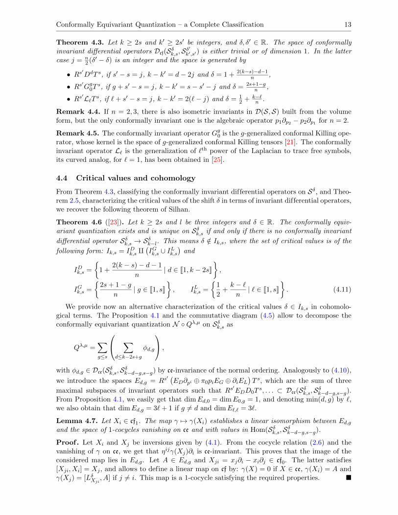
Theorem 4.3. Let k ≥ 2s and k′ ≥ 2s′ be integers, and δ, δ′ ∈ R. The space of conformallyinvariant differential operators Dcf(Sδk,s,Sδ

′k′,s′) is either trivial or of dimension 1. In the latter

case j = n2 (δ′ − δ) is an integer and the space is generated by

• Rs′DdT s, if s′ − s = j, k − k′ = d− 2j and δ = 1 + 2(k−s)−d−1n ,

• Rs′Gg0T s, if g + s′ − s = j, k − k′ = s− s′ − j and δ = 2s+1−gn ,

• Rs′L`T s, if `+ s′ − s = j, k − k′ = 2(`− j) and δ = 12 + k−`

n .

Remark 4.4. If n = 2, 3, there is also isometric invariants in D(S,S) built from the volumeform, but the only conformally invariant one is the algebraic operator p1∂p2 − p2∂p1 for n = 2.

Remark 4.5. The conformally invariant operator Gg0 is the g-generalized conformal Killing ope-rator, whose kernel is the space of g-generalized conformal Killing tensors [21]. The conformallyinvariant operator L` is the generalization of `th power of the Laplacian to trace free symbols,its curved analog, for ` = 1, has been obtained in [25].

4.4 Critical values and cohomology

From Theorem 4.3, classifying the conformally invariant differential operators on Sδ, and Theo-rem 2.5, characterizing the critical values of the shift δ in terms of invariant differential operators,we recover the following theorem of Silhan.

Theorem 4.6 ([23]). Let k ≥ 2s and l be three integers and δ ∈ R. The conformally equiv-ariant quantization exists and is unique on Sδk,s if and only if there is no conformally invariant

differential operator Sδk,s → Sδk−l. This means δ /∈ Ik,s, where the set of critical values is of the

following form: Ik,s = IDk,s q(IGk,s ∪ ILk,s

)and

IDk,s =

{1 +

2(k − s)− d− 1

n| d ∈ J1, k − 2sK

},

IGk,s =

{2s+ 1− g

n| g ∈ J1, sK

}, ILk,s =

{1

2+k − `n| ` ∈ J1, sK

}. (4.11)

We provide now an alternative characterization of the critical values δ ∈ Ik,s in cohomolo-gical terms. The Proposition 4.1 and the commutative diagram (4.5) allow to decompose theconformally equivariant quantization N ◦Qλ,µ on Sδk,s as

Qλ,µ =∑g≤s

∑d≤k−2s+g

φd,g

,

with φd,g ∈ Dce(Sδk,s,Sδk−d−g,s−g) by ce-invariance of the normal ordering. Analogously to (4.10),

we introduce the spaces Ed,g = Rs′ (ED∂pi ⊕ π0piEG ⊕ ∂iEL

)T s, which are the sum of three

maximal subspaces of invariant operators such that Rs′EDD0T

s, . . . ⊂ Dce(Sδk,s,Sδk−d−g,s−g).From Proposition 4.1, we easily get that dimEd,0 = dimE0,g = 1, and denoting min(d, g) by `,we also obtain that dimEd,g = 3`+ 1 if g 6= d and dimE`,` = 3`.

Lemma 4.7. Let Xi ∈ cf1. The map γ 7→ γ(Xi) establishes a linear isomorphism between Ed,gand the space of 1-cocycles vanishing on ce and with values in Hom(Sδk,s,Sδk−d−g,s−g).

Proof. Let Xi and Xj be inversions given by (4.1). From the cocycle relation (2.6) and thevanishing of γ on ce, we get that ηijγ(Xj)∂i is ce-invariant. This proves that the image of theconsidered map lies in Ed,g. Let A ∈ Ed,g and Xji = xj∂i − xi∂j ∈ cf0. The latter satisfies[Xji, Xi] = Xj , and allows to define a linear map on cf by: γ(X) = 0 if X ∈ ce, γ(Xi) = A andγ(Xj) = [LδXji , A] if j 6= i. This map is a 1-cocycle satisfying the required properties. �

14 J.-P. Michel

Proposition 4.8. The relative cohomology space H1(cf, ce; Hom(Sδk,s,Sδ)) changes of dimension

exactly for the critical values δ ∈ Ik,s. Then it rises by one, or two if δ ∈ IGk,s∩ILk,s. In particular,the 1-cocycles

γd : X 7→ ∂i(DivX)∂piDd−1, γg : X 7→ ηij∂i(DivX)Rs−gπ0pjG

g−10 T s,

are nontrivial if and only if the operators Dd and Rs−gGg0Ts are cf-invariant.

Proof. According to the proof of the previous Lemma, if [γ] ∈ H1(cf, ce; Hom(Sδk,s,Sδ)), then

ηij∂iγ(Xj) is ce-invariant. Consequently, the space H1(cf, ce; Hom(Sδk,s,Sδ)) is the direct sum

of the spaces H1(cf, ce; Hom(Sδk,s,Sδk−d−g,s−g)) for g ≤ s and d ≤ k − 2s + g. The spaces ofcorresponding 1-cocycles have just been identified to the spaces Ed,g, whose dimension is knownand independent of δ. The spaces of corresponding 1-coboundaries have a dimension equal tothat of Dce(Sδk,s,Sδk−d−g,s−g) minus the one of the subspaces of cf-invariant elements. The latteris zero generically, except for the critical values δ ∈ Ik,s, hence the result.

For generic δ, the two given maps γd and γg are 1-coboundaries, proportional to the differen-tial of the operators Dd and, respectively, Rs−gGg0T

s. Consequently, they define 1-cocycles forevery δ ∈ R. Since they vanish on ce, they are trivial only if they are of the form X 7→ [A,LδX ],with A ∈ Dce(Sδk,s,Sδk′,s′) for the adapted values of k′ and s′. This space reduces to 0 if Dd and

Rs−gGg0Ts are cf-invariant, leading to the announced result. �

4.5 Resonances and conformally invariant differential operators

The pairs of weights (λ, µ) for which the conformally equivariant quantization exists are com-pletely known only on symbols of degrees 2 and 3 in the momenta [8, 18]. Such a pair is calleda resonance and in the known cases there are a finite number of resonances for a given criticalvalue of the shift δ = µ−λ. We extend those results to the general case and provide a completeclassification for existence of the conformally equivariant quantization.

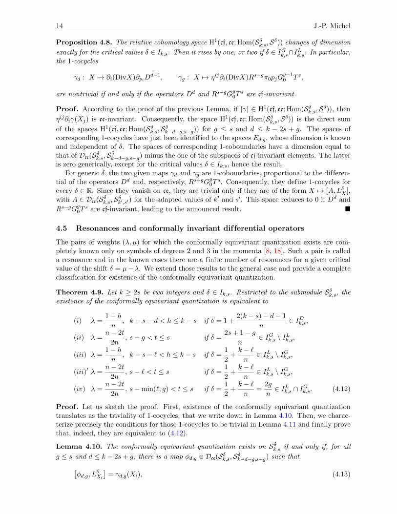
Theorem 4.9. Let k ≥ 2s be two integers and δ ∈ Ik,s. Restricted to the submodule Sδk,s, theexistence of the conformally equivariant quantization is equivalent to

(i) λ =1− hn

, k − s− d < h ≤ k − s if δ = 1 +2(k − s)− d− 1

n∈ IDk,s,

(ii) λ =n− 2t

2n, s− g < t ≤ s if δ =

2s+ 1− gn

∈ IGk,s \ ILk,s,

(iii) λ =1− hn

, k − s− ` < h ≤ k − s if δ =1

2+k − `n∈ ILk,s \ IGk,s,

(iii)′ λ =n− 2t

2n, s− ` < t ≤ s if δ =

1

2+k − `n∈ ILk,s \ IGk,s,

(iv) λ =n− 2t

2n, s−min(`, g) < t ≤ s if δ =

1

2+k − `n

=2g

n∈ ILk,s ∩ IGk,s. (4.12)

Proof. Let us sketch the proof. First, existence of the conformally equivariant quantizationtranslates as the triviality of 1-cocycles, that we write down in Lemma 4.10. Then, we charac-terize precisely the conditions for those 1-cocycles to be trivial in Lemma 4.11 and finally provethat, indeed, they are equivalent to (4.12).

Lemma 4.10. The conformally equivariant quantization exists on Sδk,s if and only if, for all

g ≤ s and d ≤ k − 2s+ g, there is a map φd,g ∈ Dce(Sδk,s,Sδk−d−g,s−g) such that[φd,g, L

δXi

]= γd,g(Xi), (4.13)

Conformally Equivariant Quantization – a Complete Classification 15

where the right hand side is the corestriction of (Lλ,µXi − LδXi

) ◦ (φd,g−1 + φd−1,g) to the subspace

Sδk−d−g,s−g. It is given by

γd,g(Xi) = Gk+1−d−gs+1−g (λ)φd,g−1 + Dk+1−d−g

s−g (λ)φd−1,g, (4.14)

and for any 2s′ ≤ k′ the operators Gk′s′ (λ) : Sδk′,s′ → Sδk′−1,s′−1 and Dk′s′ (λ) : Sδk′,s′ → Sδk′−1,s′

vanish if and only if λ = n−2s′

2n and λ = 1−(k′−s′)n respectively.

Proof. The equation (4.13) is simply the projection of equation (2.8) on the space Sδk−d−g,s−g.Hence, we just have to get the explicit expression of γd,g(Xi). For that, we need to decompose

the operator Lλ,µXi − LδXi

given in (4.2). Let RsQ ∈ Sδk,s, so that Q is in the kernel of T . Using

the decomposition piQ = π0(piQ) + 2ρk−2s+1,1

R∂piQ, where ρk,s = 2s(n + 2(k − s − 1)) is the

eigenvalue of RT and π0 denotes the projection on kerT , we obtain(Lλ,µXi − L

δXi

)(RsQ) = 2s(2nλ+ 2s− n)Rs−1π0(piQ)

+

(2nλ+ 2(k − 1) + 2s

2nλ− 2s− nn+ 2(k − 2s− 1)

)Rs∂piQ.

Both coefficients are affine functions in λ vanishing for the announced values of λ, and we haveRs−1π0(piQ) ∈ Sδk−1,s−1 and Rs∂piQ ∈ Sδk−1,s. Hence, we get the announced expression (4.14)for γd,g(Xi). �

Lemma 4.11. Existence of the conformally equivariant quantization on Sδk,s is equivalent to:

γd,0 = 0, γ0,g = 0 or γ`,`(Xi) has no component in ∂iRs−`L`−1

0 T s if, respectively, Dd, Rs−gGg0Ts

or Rs−`L`T s is conformally invariant.

Proof. Using the preceding lemma, we know that the conformally equivariant quantizationexists if and only if the 1-cocycles γd,g are trivial. But resorting to the proof of Theorem 2.5,this is the case except when there is a conformally invariant operator in Homce(Sδk,s,Sδk−d−g,s−g).Hence, the previous classification of such operators shows that the only nontrivial 1-cocycle isγd,0, γ0,g or γ`,` if respectively Dd, Rs−gGg0T

s or Rs−`L`T s is conformally invariant. Since thepreviously introduced spaces of 1-cocycles Ed,0 and E0,g are unidimensional, Proposition 4.8implies that γd,0 and γ0,g are trivial if and only if they vanish. It remains to handle the caseof γ`,`. We suppose that Rs−`L`T s is conformally invariant for the shift δ. Let us denote by Cδ

′

the space of 1-coboundaries [Homce(Sδ′k,s,Sδ

′k−`,s−`), L

δ′ ]. Generically, γ`,` is a 1-coboundary, so it

pertains to the space limδ′→δ

Cδ′

= Cδ⊕R. The linear form giving the component in ∂iRs−`L`−1

0 T s

vanishes precisely on the subspace of 1-coboundaries Cδ, and thus γ`,` is trivial if and only if itpertains to its kernel. �

We are ready now to prove the theorem. In each of the four cases in (4.12), i.e. for eachcritical value δ, we determine the operators Gk′

s′ (λ) and Dk′′s′′ (λ) which should vanish, so that theprevious constraints on the 1-cocycles γd,0, γ0,g, γ`,` are satisfied.

The instances δ ∈ IDk,s and δ ∈ IGk,s are treated like in the projective case, the concerned space

Homce being unidimensional. In the first case, it exists d ≤ k − 2s such that Dd is conformallyinvariant, and Lemma 4.11 implies that γd,0 = 0. Using equation (4.14), we obtain by inductionthat Dh+s

s (λ) = 0 for some k− s− d < h ≤ k− s, hence the result (i) of (4.12). If δ ∈ IGk,s, then

it exists g ≤ s such that Rs−gGg0Ts is conformally invariant. Similarly we must have γ0,g = 0

and then, by induction, Gk−s+tt (λ) = 0 for some s− g < t ≤ s. The result (ii) of (4.12) follows.

The instance δ ∈ ILk,s is more involved, and relies, as Lemma 4.2, on independence of mono-

mials Gg0Dd0L

`0 for different exponents `. In that case, there exists ` ≤ s such that Rs−`L`T s

16 J.-P. Michel

is conformally invariant and Lemma 4.11 implies that γ`,` must have no component along∂iR

s−`L`−10 T s. We deduce from the formula (4.14) that either Dk+1−2`

s−` = 0 or φ`−1,` has no

component in Rs−`G0L`−10 T s. Then, a straightforward induction proves that all the paths in

the following diagram (4.15) from Id to L`0 have a vanishing label on at least one of its arrows.For simplicity we do not write the appropriate powers of R and T .

IdGks (λ)

yyG0

Gk−1s−1 (λ)

yy

Dk−1s−1 (λ)

$$G2

0

{{

Dk−2s−2 (λ)

%%

L0Gk−2s−1 (λ)

zz· · ·

Gk−`+1s−`+1 (λ)

~~

G0L0

yy $$G`0

Dk−`s−` (λ)��

· · ·

%%

· · ·

{{· · ·

""

G0L`−20

Gk−2l+3s−`+1 (λ)

zz

Dk−2`+3s−`+1 (λ)

##G2

0L`−20

Dk−2`−2s−` (λ) $$

L`−10

Gk−2l−2s−`+1 (λ)

{{G0L

`−10

Dk−2`+1s−` (λ) ##

L`0

(4.15)

Since Dk−ls−l (λ) and Dks(λ) vanish for the same value of λ, as well as Gks(λ) and Gk′

s (λ), we

finally get that, necessarily, Gk−s+tt (λ) = 0 or Dh+s

s (λ) = 0 for respectively s − ` < t ≤ s andk − s− ` < h ≤ k − s. Hence, we end with the results (iii) and (iii)′ of (4.12) for δ ∈ ILk,s \ IGk,s.

At least, we suppose that δ ∈ ILk,s ∩ IGk,s. Then, it exists g, ` ≤ s satisfying the relation

δ = 12 + k−`

n = 2gn . We deduce that λ must satisfy simultaneously the conditions (ii) and

(iii)/(iii)′ in (4.12) and that leads precisely to (iv). �

The last part of the proof of Theorem 4.9 shows that each λ given in (4.12) corresponds to thevanishing of an operator G or D, i.e. to the vanishing of a certain restriction of Lλ,µ − Lδ. TheLemma 3.3 allows then to deduce existence of conformally invariant differential operators on λ-densities, for each resonance λ in (4.12). They organize in two families: the powers of Laplacian

∆t : Fn−2t2n → F

n+2t2n and the operators π0G

h : F1−hn → S

1−hn

h,0 which are built from the operator

G = pi∂i, introduced in (3.5). The latter is dual to the conformal Killing operator G arising inLemma 4.2. By Weyl’s theory of invariants or by the general classification in [2, 3], these are allthe conformally invariant differential operators on λ-densities. Hence, we can reformulate theTheorem 4.9 along the lines of Kroeske’s paradigm. Notice that it is done a posteriori, contraryto the Theorem 2.5.

Conformally Equivariant Quantization – a Complete Classification 17

Theorem 4.12. The conformally equivariant quantization Qλ,µ : Sδk,s ⊗Fλ → Fµ exists and is

unique except when there is a conformally invariant differential operator: Sδk,s → Sδk−l,s−r. Then,

Qλ,µ exists if and only if there is a conformally invariant differential operator from Fλ to sectionsof a homogeneous bundle V, whose principal symbol lies in S−λh,t ⊗Γ(V) with Dce(Sδk,s,Sδh,t) 6= {0}and Dce(Sδk−l,s−r,Sδh,t) = {0}.

Silhan provides in [23] an explicit construction for the conformally equivariant quantizationwhen the shift δ is not one of the critical values (4.11), and also two alternative constructionsin the critical cases. In the next two propositions, we prove that they allow to handle all theremaining cases of existence, when (λ, λ+ δ) is a resonance (4.12).

Proposition 4.13. In the three cases (ii), (iii), (iv) of (4.12), the operator ∆t : Fλ → Fλ+ 2tn

is conformally invariant. The commutative diagram

Sδk,s ⊗Fλ

''

aT t⊗∆t// Sδ−

2tn

k−2t,s−t ⊗Fλ+ 2t

n

Qλ+2tn , µ

��Fµ

defines then a conformally equivariant quantization on Sδk,s for a well-chosen constant a ∈ R.

Proof. The operator a T t above is conformally invariant, and a can be chosen such that theequality aRtT t = Id holds on Sδk,s, ensuring the good normalization. Moreover, the conformally

equivariant quantization Qλ+ 2tn, µ is well defined on Sδ−

2tn

k−2t,s−t by Theorem 4.6. �

Let us introduce a refinement of the filtration of Dλ,µ, which already appears in [7]. Namely,

we denote by Dλ,µk,s the subspace of Dλ,µk given by the image of⊕

0≤s−r≤k−l Sδl,r under the normal

ordering. The expression (4.2) of the action of cf shows thatDλ,µk,s is in fact a cf-submodule ofDλ,µk .

The subspaces Sδl,r arising in its definition are characterized equivalently by Dce(Sδk,s,Sδl,r) 6= 0 or,with the notation of Lemma 4.10, by their presence in the following tree, analogous to previousones (4.6) and (4.15),

Sδk,sGks (λ)

{{ Dks (λ) ""Sδk−1,s−1

Gk−1s−1 (λ)

zz Dk−1s−1 (λ) $$

Sδk−1,sGk−1s (λ)

{{ Dk−1s (λ) ##

· · · · · · · · ·

We can restrict the differential operators obtained by morphism (ια)j , defined in (3.6), to

traceless tensors. The resulting morphism of cf-modules (ια)j0 : Dλ,µk,s → Dλ,µk−h(Sλh,0,Fµ) has

clearly a nontrivial kernel, which is equal to Dλ,µj−1+r,r ⊃ Dλ,µj−1 if r = min(s, j − 1). This leads to

the following result, similar to Proposition 3.4 dealing with the projective case.

18 J.-P. Michel

Proposition 4.14. In the two cases (i) and (iii)′ of (4.12), the operator π0Gh : Fλ → Sλh,0 is

conformally invariant. The commutative diagram

Sδk,s ⊗Fλ

++

Qλ,µk,h⊗Id// Dλ,µk,s /D

λ,µk−h,s ⊗F

λ(ια)h0⊗π0Gh // Dλ,µk−h(Sλh,0,Fµ)⊗ Sλh,0

��Fµ

defines then a conformally equivariant quantization on Sδk,s.

Proof. In view of the definition of h, there is no obstruction to the existence of the partialconformally equivariant quantization Qλ,µk,h . Using the conformal invariance of π0G

h and of (ια)h0 ,we get the result. �

4.6 Example: conformally equivariant quantization of symbols of degree 3

The conformally equivariant quantization as been explicitly determined up to order 3 in themomenta by Loubon Djounga in [18]. We give here for each submodule Sδk,s, with k ≤ 3, theconformally invariant operators acting on it, the corresponding critical values of the shift δ, theresonances (λ, λ+ δ) and the associated conformally invariant operators on Fλ.

Space Op. Inv. on Sδk,s δ λ Op. Inv. on Fλ

Sδ1 D 1 0 G

Sδ2,0 D n+2n − 1

n G2

D2 n+1n − 1

n , 0 G2, G

Sδ2,1 G0T2n

n−22n ∆

L0Tn+22n

n−22n , 0 ∆, G

Sδ3,0 D n+4n − 2

n G3

D2 n+3n − 2

n ,−1n G3, G2

D3 n+2n − 2

n ,−1n , 0 G3, G2, G

Sδ3,1 RDT n+2n − 1

n G2

G0T2n

n−22n ∆

L1Tn+2n

n−22n ,−

1n , 0 ∆, G2, G

Let δ be one of the above critical values. If we consider the conformally equivariant quantizationon the whole space Sδ3⊕Sδ2⊕Sδ1⊕Sδ0 , as in [18], then it will exist only for the values of λ appearingin each row where δ is present. Thus, we recover precisely the result of [18].

5 Prospects

We have proven in the setting of IFFT-equivariant quantization, introduced in [4], that uniqueexistence of the quantization map is lost if and only if there is an invariant differential operator

Conformally Equivariant Quantization – a Complete Classification 19

on the space of symbols. The work of Cap and Silhan [6] allows to trivially extend this resultto IFFT-equivariant quantization with values in differential operators acting on homogeneousirreducible bundles. It remains then to characterize when equivariant quantization exists but isnot unique. We have done it only for projectively and conformally equivariant quantizations,with values in Dλ,µ, in terms of existence of an invariant differential operator on the module Fλof λ-densities. In the light of these both examples we propose the following method to linkresonances with invariant operators on the source space (e.g. Fλ).

• To each invariant differential operator acting on the space of symbols corresponds a non-trivial 1-cocycle γ.

• The latter obstructs the existence of the equivariant quantization except for a finite numberof values of λ.

• For those values, a certain restriction of the operator Lλ,µ − Lδ vanishes.

• An invariant differential operator on the source space can then be built, and we obtain allof them in this way.

• An equivariant quantization can be design from those invariant operators.

We hope that this will lead to the proof of the point (2) in the following conjecture, the point (1)being Theorem 2.6.

Conjecture 5.1. Let g be an IFFT-algebra, V, W be irreducible homogeneous bundles and Ba submodule of Sδk(V,W). The g-equivariant quantization B⊗(Γ(V)⊗Fλ) −→ Γ(W)⊗Fµsatisfiesthe following properties:

1) it does not exist or is not unique if and only if, for 1 ≤ l ≤ k, there is a g-invariantdifferential operator: B → C, with C a submodule of Sδk−l(V,W),

2) for such δ, the g-equivariant quantization exists if and only if there is a g-invariant dif-ferential operator on Γ(V) ⊗ Fλ, whose principal symbol lies in A and satisfies the bothconditions Dg−1⊕g0(B,A) 6= 0 and Dg−1⊕g0(C,A) = 0.

The next step will be to generalize such a result for g-invariant bidifferential pairings, whichare bidifferential operators Γ(V)⊗ Γ(W)→ Γ(T ), where V, W, T are irreducible homogeneousbundles. Let us discuss the peculiar case of the generalized transvectants or Rankin–Cohenbrackets. It has been proved in [22] that there exists a unique conformally invariant bidifferential

operator of order 2k acting on λ- and µ-densities, Bλ,µ2k : Fλ⊗Fµ → Fλ+µ+ 2k

n , if and only if theweights λ and µ do not pertain to the set of exceptional values {n−2k

2n , . . . , n−22n }∪ {

2−2kn , . . . , 0}.

Remarkably they precisely coincide with the resonances of the conformally equivariant quanti-zation. For those exceptional values, we can construct new generalized transvectants from the

conformally invariant operators ∆` and Gg0. Explicitly, they are given by Bλ+ 2`

n,µ

2(k−`) ◦ (∆` ⊗ Id)

if ` ≤ k and λ ∈ {n−2k2n , . . . , n−2

2n }, and by Qλ,µ ◦ (Gg0 ⊗ Id) if g ≤ 2k − 1, µ is generic and

λ ∈ {2−2kn , . . . , 0}. A tight link between bidifferential and differential invariant operators shows

up one more time. The same kind of idea is used in [1], where new conformally invariant tri-linear forms on tensor densities are built from the invariant operators ∆`. To conclude, Kroeske’sparadigm definitely asks for deeper investigations.

Acknowledgements

It is a pleasure to acknowledge Christian Duval, Pierre Mathonet and Valentin Ovsienko forfruitful discussions and the referees for suggesting numerous improvements. I thank the Luxem-bourgian NRF for support via the AFR grant PDR-09-063.

20 J.-P. Michel

References

[1] Beckmann R., Clerc J.L., Singular invariant trilinear forms and covariant (bi-)differential operators underthe conformal group, J. Funct. Anal. 262 (2012), 4341–4376.

[2] Boe B.D., Collingwood D.H., A comparison theory for the structure of induced representations, J. Algebra94 (1985), 511–545.

[3] Boe B.D., Collingwood D.H., A comparison theory for the structure of induced representations. II, Math. Z.190 (1985), 1–11.

[4] Boniver F., Mathonet P., IFFT-equivariant quantizations, J. Geom. Phys. 56 (2006), 712–730,math.RT/0109032.

[5] Boniver F., Mathonet P., Maximal subalgebras of vector fields for equivariant quantizations, J. Math. Phys.42 (2001), 582–589, math.DG/0009239.

[6] Cap A., Silhan J., Equivariant quantizations for AHS-structures, Adv. Math. 224 (2010), 1717–1734,arXiv:0904.3278.

[7] Duval C., Lecomte P., Ovsienko V., Conformally equivariant quantization: existence and uniqueness, Ann.Inst. Fourier (Grenoble) 49 (1999), 1999–2029, math.DG/9902032.

[8] Duval C., Ovsienko V., Conformally equivariant quantum Hamiltonians, Selecta Math. (N.S.) 7 (2001),291–320, math.DG/9801122.

[9] Duval C., Ovsienko V., Projectively equivariant quantization and symbol calculus: noncommutative hyper-geometric functions, Lett. Math. Phys. 57 (2001), 61–67, math.QA/0103096.

[10] Eastwood M., Slovak J., Semiholonomic Verma modules, J. Algebra 197 (1997), 424–448.

[11] Eastwood M.G., Rice J.W., Conformally invariant differential operators on Minkowski space and theircurved analogues, Comm. Math. Phys. 109 (1987), 207–228, Erratum, Comm. Math. Phys. 144 (1992),213.

[12] Fuks D.B., Cohomology of infinite-dimensional Lie algebras, Contemporary Soviet Mathematics, ConsultantsBureau, New York, 1986.

[13] Kobayashi S., Nagano T., On filtered Lie algebras and geometric structures. I, J. Math. Mech. 13 (1964),875–907.

[14] Kroeske J., Invariant bilinear differential pairings on parabolic geometries, Ph.D. thesis, University of Ade-laide, 2008, arXiv:0904.3311.

[15] Kroeske J., Invariant differential pairings, Acta Math. Univ. Comenian. (N.S.) 77 (2008), 215–244,math.DG/0703866.

[16] Lecomte P.B.A., On the cohomology of sl(m + 1,R) acting on differential operators and sl(m + 1,R)-equivariant symbol, Indag. Math. (N.S.) 11 (2000), 95–114, math.DG/9801121.

[17] Lecomte P.B.A., Ovsienko V.Y., Projectively equivariant symbol calculus, Lett. Math. Phys. 49 (1999),173–196, math.DG/9809061.

[18] Loubon Djounga S.E., Modules of third-order differential operators on a conformally flat manifold, J. Geom.Phys. 37 (2001), 251–261.

[19] Mathonet P., Radoux F., Cartan connections and natural and projectively equivariant quantizations,J. Lond. Math. Soc. (2) 76 (2007), 87–104, math.DG/0606556.

[20] Mathonet P., Radoux F., Existence of natural and conformally invariant quantizations of arbitrary symbols,J. Nonlinear Math. Phys. 17 (2010), 539–556, arXiv:0811.3710.

[21] Nikitin A.G., Prilipko A.I., Generalized Killing tensors and the symmetry of the Klein–Gordon–Fock equa-tion, Preprint no. 90.23, Institute of Mathematics, Kyiv, 1990, 59 pages, math-ph/0506002.

[22] Ovsienko V., Redou P., Generalized transvectants-Rankin–Cohen brackets, Lett. Math. Phys. 63 (2003),19–28, math.DG/0104232.

[23] Silhan J., Conformally invariant quantization – towards complete classification, arXiv:0903.4798.

[24] Weyl H., The classical groups. Their invariants and representations, Princeton Landmarks in Mathematics,Princeton University Press, Princeton, NJ, 1997.

[25] Wunsch V., On conformally invariant differential operators, Math. Nachr. 129 (1986), 269–281.