ISRN LUTMDN/TMHP-17/5391-SE

ISSN 0282-1990

Transient model of a driven

compressor

LUND UNIVERSITY

Rasmus Johnsson

Sebastian Norén

Thesis for the Degree of Master of Science

Division of Thermal Power Engineering

Department of Energy Science

Lund Institute of Technology | Lund University

Transient model of a driven compressor

Transient model of a driven compressor

by Rasmus Johnsson and Sebastian Norén

Thesis for the Degree of Master of ScienceThesis advisors: Assoc. Prof. Marcus Thern, Anna Sjunnesson

This thesis for the degree of Master of Science in Engineering has been conducted atthe Division of Thermal Power Engineering, Department of Energy Sciences, LTH –Lund University and at Siemens Industrial Turbomachinery AB. Supervisor at SiemensIndustrial Turbomachinery AB: Anna Sjunnesson; supervisor at LU-LTH: Assoc. Prof.Marcus Thern; examiner at LU-LTH: Prof. Magnus Genrup.

© Rasmus Johnsson and Sebastian Norén 2017

Division of Thermal Power Engineering, Department of Energy ScienceBox 118, 221 00 Lundwww.energy.lth.se

issn: <0282-1990>

Printed in Sweden by Media-Tryck, Lund University, Lund 2017

”Education is what remains after one has forgotten what one has learned in school”- Albert Einstein

Abstract

Industrial gas turbines are widely used in different applications. These can be dividedinto two main categories; power generation (PG) and mechanical drive (MD). To beable to predict the performance of the system, Siemens has during the years developedsimulation models for both steady state and transient operation. These models are mainlydesigned for PG, so there is a need for new MD models. An MD model includes a gasturbine, a driven component, in this case a compressor, and auxiliary systems whichensures stable operation and avoid rotating stall and surge in the compressor.

The purpose of this thesis is to develop a transient model of a driven compressor basedon characteristics and connect it with the existing dynamic gas turbine model of theSiemens Gas Turbine 750 (SGT-750) in Dymola. Auxiliary systems are developed forboth the compressor system and for the compressor train in order to reflect the realityand get reliable simulation results. An analysis is performed to study the behaviour ofthe compressor train when controller and physical parameters are changed.

The developed compressor model is based on the existing basic compressor modeldeveloped by Siemens. Compressor maps from the reference project El-Encino wereimplemented in the model and were verified against data sheets and the model was thenconnected to the existing SGT-750 model in Dymola. New controllers were developedto ensure reliable operation of the compressor train and the complete model was thentuned in and verified towards measured data from two different sites with the SGT-700as the driving component. Different cases were simulated to assure stable operation forvarying starting conditions and to study the behaviour of the compressor train.

The verification shows that the developed model corresponds to reality with deviationswithin the approved area, with regard of the limitations of the project. The model nowmakes it possible to study the gas turbine behaviour in an MD application with theSGT-750 as the driving component. The configuration of the gas turbine control systemmakes it possible to use it in different applications with different gas turbines, bothfor PG and MD. The behaviour analysis shows that a lower fuel ramp during start-upincreases the stability of the compressor train. It also indicates that the power turbineacceleration controller could be redundant for certain cases but further analysis is neededin the matter. Due to the focus of the project and limitations in Dymola, more work isneeded to ensure accuracy of all parameter values. There are improvement opportunitiesin the program’s basic thermodynamic functions, which is a part of the future work.

Keywords: gas turbine, modelling, Dymola, SGT-750, mechanical drive, compressortrain, thermodynamics, performance.

i

Sammanfattning

Industriella gasturbiner används i många olika applikationer och tillämpningar. Dessakan delas in i två huvudkategorier; Kraftgenerering (PG) och mekanisk drift (MD). Föratt kunna förutsäga systemens prestanda har Siemens genom åren utvecklat simulerings-modeller för både steady state och transienta förlopp. Dessa modeller är huvudsakligenavsedda för PG, så det finns ett behov av nya MD-modeller. En MD-modell innehållervanligtvis en gasturbin, den drivna komponenten, i detta fall en kompressor, samt hjälp-system. Hjälpsystemen till modellen ska säkerställa stabil drift och undvika Rotatingstall och Surge i kompressorn.

I detta examensarbete utvecklas en transient modell av en driven kompressor baseradpå karaktäristik, som sammankopplas med den befintliga dynamiska gasturbinmodellenför Siemens Gas Turbine 750 (SGT-750) i Dymola. Hjälpsystem utvecklas för bådekompressorsystemet och kompressortåget för att återspegla verkligheten och erhållapålitliga simuleringsresultat. En analys utförs för att se hur kompressortåget svarar påändringar av fysiska parametrar och parametrar i kontrollsystemet.

Kompressormodellen som utvecklas baseras på den befintliga baskompressormodellenutvecklad av Siemens. Kompressorkartor från referensprojektet El-Encino implemente-rades i modellen som därefter verifierades med hjälp av datablad och sammankoppladesmed den befintliga SGT-750 modellen i Dymola. Nya regulatorer utvecklades för attfå tillförlitliga simuleringar av kompressortåget, den slutliga modellen trimmades se-dan in och verifierades mot uppmätta data från två olika siter med SGT-700 som dendrivande komponenten. Olika fall simulerades för att säkerställa stabil drift vid olikastartförhållanden och för att studera beteendet hos kompressortåget.

Verifieringen visar att modellen motsvarar verkligheten med avvikelser inom ett godkäntområde, med tanke på begränsningarna i projektet. Modellen gör det möjligt att studeragasturbinens beteende i enMD-applikationmed SGT-750 som den drivande komponenten.Styrsystemets utformning gör det möjligt att använda det i andra applikationer och medandra gasturbiner, både för PG och MD. Beteendeanalysen visar att en lägre bränslerampger en stabilare start av kompressortåget. Den indikerar också att regulatorn somkontrollerar accelerationen av kraftturbinen är överflödig i vissa fall. Dock bör dettaanalyseras vidare. På grund av arbetets avgränsningar samt begränsningar i Dymolabehövs mer arbete för att kunna säkerställa noggrannheten av alla parametervärden.Förbättringsmöjligheter finns i programmets grundläggande termodynamiska funktionervilka bör utvecklas ytterligare.

Nyckelord: gasturbin, modellering, Dymola, SGT-750, mekanisk drift, kompressortåg,termodynamik, prestanda.

ii

Acknowledgements

There are many people that have made this project possible, both at Siemens IndustrialTurbomachinery AB (SIT) and at Lund University (LU). If all is to be mentioned the listwould be very long.

Our biggest gratitude goes to Anna Sjunnesson, our supervisor at SIT. She has helped usfrom the first day and led us through the whole project. It has been an honour to be guidedby her knowledge and experience, when meeting both silly and complex challenges.

We would like to thank the department manager Lennart Näs for giving us the opportunityto be a part of the performance department, and including us in the everyday work,Dr. Klas Jonshagen for his patient and understandable way of explaining complexthermodynamic problems.

We would also like to thank the whole performance department for their help andguidance throughout the project and for making us feel welcome at Siemens.

Many thanks to Prof. Magnus Genrup, who first introduced us to the world of turbinesand created the opportunity to write this master thesis at SIT. We also want to thank oursupervisor at LU, Assoc. Prof. Marcus Thern, for his guidance throughout the project.Our gratitude also goes to all employees at LU that have given us the knowledge neededin this project and in our future life as Mechanical Engineers.

Last but not least, thanks to our families and loved ones for all the support during theyears!

Rasmus Johnsson Sebastian NorénFinspång 2017-06-12 Finspång 2017-06-12

iii

Nomenclature

Latin symbols Unit Description

A [m2] Area

C [m s−1] Velocity

cθ [m s−1] Tangential speed

cp [J kg−1 K−1] Specific heat capacity, constant pressure

cv [J kg−1 K−1] Specific heat capacity, constant volume

D [m] Diameter

E [kJ] Energy

H [J] Enthalpy

h [J kg−1] Specific enthalpy

J [kg m2] Rotational inertia

M [kg mol−1] Molar mass

m [kg] Mass

Ûm [kg s−1] Mass flow

N [rpm] Rotational speed

n [-] Number of inlet guide vanes

np [-] Number of purges required

P [W] Power

p [bar] Pressure

Q [J] HeatÛQ [kJ s−1] Heat flow

R [J kg−1 K−1] Gas constant

R [J mol−1 K−1] The universal gas constant

r [m] Radius

s [J kg−1 K−1] Specific entropy

T [K] Temperature

U [J] Internal energy

iv

Unit Description

u [J kg−1] Specific internal energy

Vw [m s−1] Tangential velocity

VGT [m3] Volume of the gas turbine

VpurgeE xsys [m3] Volume of the exhaust systemÛVpurgeE xsys [m3 s−1] Air flow through exhaust system during purgeÛVpurgeGT [m3 s−1] Air flow through gas turbine during purge

v [m3 kg−1] Specific volume

W [J] Work

Z [m3 s−1] Compressibility

Greek symbols Unit Description

γ [-] Ratio between cp and cv

∆ [-] Difference

η [-] Efficiency

ρ [kg m−3] Density

σ [-] Slip factor

τ [N m] Torque

ψ [-] Power input factor

Ω [rad s−1] Angular velocity

v

Contents

Abstract . . . . . . . . . . . . . . . . . . . . . . . . . . . . . . . . . . . . . iSammanfattning . . . . . . . . . . . . . . . . . . . . . . . . . . . . . . . . . iiAcknowledgements . . . . . . . . . . . . . . . . . . . . . . . . . . . . . . . iiiNomenclature . . . . . . . . . . . . . . . . . . . . . . . . . . . . . . . . . . iv

1 Introduction 11.1 Background . . . . . . . . . . . . . . . . . . . . . . . . . . . . . . . . 11.2 Objectives . . . . . . . . . . . . . . . . . . . . . . . . . . . . . . . . . 2

1.2.1 Problem definition . . . . . . . . . . . . . . . . . . . . . . . . 21.3 Limitations . . . . . . . . . . . . . . . . . . . . . . . . . . . . . . . . 21.4 Method . . . . . . . . . . . . . . . . . . . . . . . . . . . . . . . . . . 31.5 Tools . . . . . . . . . . . . . . . . . . . . . . . . . . . . . . . . . . . . 4

2 Theory 52.1 System description . . . . . . . . . . . . . . . . . . . . . . . . . . . . 5

2.1.1 Mechanical Drive . . . . . . . . . . . . . . . . . . . . . . . . . 52.1.2 Compressor system . . . . . . . . . . . . . . . . . . . . . . . . 5

2.2 Compressor . . . . . . . . . . . . . . . . . . . . . . . . . . . . . . . . 62.3 Centrifugal compressor . . . . . . . . . . . . . . . . . . . . . . . . . . 72.4 Energy and mass balance . . . . . . . . . . . . . . . . . . . . . . . . . 72.5 Ideal gas model . . . . . . . . . . . . . . . . . . . . . . . . . . . . . . 92.6 The momentum equation and the Euler work equation . . . . . . . . . . 102.7 Work done . . . . . . . . . . . . . . . . . . . . . . . . . . . . . . . . . 122.8 Compressor characteristics . . . . . . . . . . . . . . . . . . . . . . . . 132.9 Rotating stall and surge . . . . . . . . . . . . . . . . . . . . . . . . . . 172.10 Polytropic efficiency using the sT-method . . . . . . . . . . . . . . . . 182.11 Gas turbine . . . . . . . . . . . . . . . . . . . . . . . . . . . . . . . . 192.12 Heat transfer . . . . . . . . . . . . . . . . . . . . . . . . . . . . . . . . 212.13 System control . . . . . . . . . . . . . . . . . . . . . . . . . . . . . . . 22

2.13.1 Anti-surge control . . . . . . . . . . . . . . . . . . . . . . . . . 232.13.2 PID-controller . . . . . . . . . . . . . . . . . . . . . . . . . . . 23

2.14 Start-up sequence . . . . . . . . . . . . . . . . . . . . . . . . . . . . . 252.15 Purge . . . . . . . . . . . . . . . . . . . . . . . . . . . . . . . . . . . 262.16 Natural gas . . . . . . . . . . . . . . . . . . . . . . . . . . . . . . . . 272.17 El-Encino . . . . . . . . . . . . . . . . . . . . . . . . . . . . . . . . . 27

2.17.1 SGT-750 . . . . . . . . . . . . . . . . . . . . . . . . . . . . . . 28

vii

2.17.2 STC-SV . . . . . . . . . . . . . . . . . . . . . . . . . . . . . . 282.18 Tools . . . . . . . . . . . . . . . . . . . . . . . . . . . . . . . . . . . . 28

2.18.1 Dymola . . . . . . . . . . . . . . . . . . . . . . . . . . . . . . 282.18.2 SVN/GITLab . . . . . . . . . . . . . . . . . . . . . . . . . . . 292.18.3 STA-RMS . . . . . . . . . . . . . . . . . . . . . . . . . . . . . 292.18.4 WebPlotDigitizer . . . . . . . . . . . . . . . . . . . . . . . . . 292.18.5 VLE Flash . . . . . . . . . . . . . . . . . . . . . . . . . . . . . 29

3 Methodology 313.1 Literature study . . . . . . . . . . . . . . . . . . . . . . . . . . . . . . 313.2 Dymola model of compressor system . . . . . . . . . . . . . . . . . . . 32

3.2.1 Compressor . . . . . . . . . . . . . . . . . . . . . . . . . . . . 323.2.1.1 Basic Model . . . . . . . . . . . . . . . . . . . . . . 333.2.1.2 Characteristics . . . . . . . . . . . . . . . . . . . . . 33

3.2.2 Medium . . . . . . . . . . . . . . . . . . . . . . . . . . . . . . 353.2.3 Compressibility . . . . . . . . . . . . . . . . . . . . . . . . . . 353.2.4 Anti-surge loop . . . . . . . . . . . . . . . . . . . . . . . . . . 36

3.2.4.1 Control valve . . . . . . . . . . . . . . . . . . . . . . 363.2.4.2 Control system . . . . . . . . . . . . . . . . . . . . . 37

3.2.5 Check valve . . . . . . . . . . . . . . . . . . . . . . . . . . . . 383.2.6 Cooler . . . . . . . . . . . . . . . . . . . . . . . . . . . . . . . 383.2.7 Source, Sink and Volumes . . . . . . . . . . . . . . . . . . . . 393.2.8 Ideal gas model . . . . . . . . . . . . . . . . . . . . . . . . . . 39

3.3 Dymola model of gas turbine control system . . . . . . . . . . . . . . . 393.3.1 Starter motor . . . . . . . . . . . . . . . . . . . . . . . . . . . 413.3.2 Start controller - STC . . . . . . . . . . . . . . . . . . . . . . . 413.3.3 Gas generator speed limiter - NGGL . . . . . . . . . . . . . . . 413.3.4 Power turbine acceleration controller - PAC . . . . . . . . . . . 413.3.5 Frequency and load controller/Speed controller - FLC/SC . . . . 423.3.6 Mass flow controller - MFC . . . . . . . . . . . . . . . . . . . 423.3.7 Exhaust temperature limiter - T0800L . . . . . . . . . . . . . . 433.3.8 Load loss detection - LLD . . . . . . . . . . . . . . . . . . . . 433.3.9 Gas generator acceleration control - GAC . . . . . . . . . . . . 443.3.10 Flame sustain control - FSC . . . . . . . . . . . . . . . . . . . 443.3.11 Gas generator deceleration control - GDC . . . . . . . . . . . . 443.3.12 Bleed valve controller - BVC . . . . . . . . . . . . . . . . . . . 45

3.4 Implementation - Connecting the compressor system with the SGT-750 . 45

4 Verification and analysis 474.1 Verification of the compressor system . . . . . . . . . . . . . . . . . . 47

4.1.1 Compressor verification . . . . . . . . . . . . . . . . . . . . . . 484.1.2 The ideal gas model . . . . . . . . . . . . . . . . . . . . . . . . 494.1.3 Start-up . . . . . . . . . . . . . . . . . . . . . . . . . . . . . . 504.1.4 Steady state . . . . . . . . . . . . . . . . . . . . . . . . . . . . 54

4.2 Verification of the compressor train . . . . . . . . . . . . . . . . . . . . 58

viii

4.2.1 Individual plots . . . . . . . . . . . . . . . . . . . . . . . . . . 584.2.2 Compressor maps . . . . . . . . . . . . . . . . . . . . . . . . . 624.2.3 Site verification . . . . . . . . . . . . . . . . . . . . . . . . . . 64

5 Behaviour analysis 675.1 Fuel ramp in STC - a) . . . . . . . . . . . . . . . . . . . . . . . . . . . 675.2 Rotational inertia - b) . . . . . . . . . . . . . . . . . . . . . . . . . . . 695.3 Deactivation of PAC - c) . . . . . . . . . . . . . . . . . . . . . . . . . 725.4 Gas generator acceleration in NGGL - d) . . . . . . . . . . . . . . . . . 73

6 Discussion 756.1 Compressor model . . . . . . . . . . . . . . . . . . . . . . . . . . . . 756.2 Compressor train . . . . . . . . . . . . . . . . . . . . . . . . . . . . . 756.3 Verification . . . . . . . . . . . . . . . . . . . . . . . . . . . . . . . . 76

6.3.1 Compressor system . . . . . . . . . . . . . . . . . . . . . . . . 766.3.2 Compressor train . . . . . . . . . . . . . . . . . . . . . . . . . 776.3.3 Compressor maps . . . . . . . . . . . . . . . . . . . . . . . . . 776.3.4 Eischleben and Port Said . . . . . . . . . . . . . . . . . . . . . 776.3.5 Behaviour analysis . . . . . . . . . . . . . . . . . . . . . . . . 78

7 Conclusions 798 Future work 819 References 83

ix

1. Introduction

For decades Finspång has been a center for industrial manufacturing. The first millstarted in the 16th century and flourished with the De Geer family in charge for over 200years. After a long period of being a major cannon producer for armies in Sweden andEurope the mill had to close in the early 20th century due to competition and the estatewas divided into several parts. Two brothers named Birger and Fredrik Ljungström hadjust founded the company STAL (Svenska Turbinfabrik AB Ljungström) in Stockholmduring this time. The brothers saw the potential of Finspångs favorable location and theunused facilities and competence in the area, so they started the production of steamturbines in Finspång. This was the start of the turbine production era in Finspång [1].In 1953 the first gas turbine order was initiated at STAL and a new business area grewwithin the company. Many company configurations have followed since then but in2003 Siemens acquired the company and formed Siemens Industrial Turbomachinery,SIT. In 2013, 100 years since the start of STAL, the company had produced around2300 steam turbines, 700 gas turbines and consisted of almost 3000 employees [2]. Themain business of SIT today is production, development, service and maintenance of gasturbines.

1.1 Background

The most common use of an industrial gas turbine is to produce electricity, in a so calledpower generation (PG) application. Another area of use is to let the gas turbine drivea compressor system and create a compressor train. These compressor trains are usedin different applications all over the world. It is common to use compressor trains fortransportation of gases, one example of that is transportation of natural gas in pipelines.The gas needs high pressure to be able to travel through the pipeline, and it is desirableto have as long distance between the pump stations as possible. This is why compressorstations with high power output is advantageous. These compressors are in most casesdriven by one or several gas turbines, but they can also be driven by an electrical motor.The characteristic preference for both these drivers are that their speed can vary overa large range. This is one of the reasons of why it is important to be able to predict

1

Objectives

the systems performance with transient operation, which partly is done in simulationprograms [3].

Siemens has during the years developed many transient gas turbine models for calculatingperformance parameters as temperature, pressure, mass flow and power during transientcourses. These are modelled for PG, and not for applications. The MD causes variationsof power turbine speed, which changes the system behaviour. A new model for this willmake it possible to answer future questions about transient performance in compressorapplications and optimize its control system.

During start-up of a compressor driven by a gas turbine there are some phenomena thatneeds to be avoided. One of this is surge, which occurs when the mass flow is too lowand the compressor is unable to produce the required discharge pressure which willemphasize a thermal block in the compressor. The surge phenomena will be explainedin detail later in this report. Surge is very harmful for the machine and could cause fatalmaterial damages and large costs. A reliable simulation which gives accurate informationabout a correct start-up sequence can prevent this and is therefore indispensable.

1.2 Objectives

The purpose of this thesis is to develop a transient model of a driven compressor, basedon characteristics. This model will be implemented by connecting it with the model forSiemens Gas Turbine 750 (SGT-750) in order to analyse the behaviour of a completecompressor train during start-up.

1.2.1 Problem definition

The following questions will be analysed and answered in this thesis:

• How well does the developed model correspond to reality?

• How will the gas turbine respond to changes of controller and physical parametersduring start-up?

1.3 Limitations

The limitations of the project are listed below:

• The compressor model will mainly be used for simulating the gas turbine behaviourand the compressor models requirement will be put with respect to this.

2

1. INTRODUCTION

• The compressor model that will be built is adapted for one specific gas turbine.Despite this, the model will be designed in a way that makes it easy to adapt witha different gas turbine model. This might be advantageous for the future.

• Only necessary changes will be made in the gas turbine model to implement thecompressor in this project.

• Only chosen components of the compressor’s auxiliary system, which affect theperformance of the gas turbine, will be modelled.

• Only components of the control system that affect the running of the compressoror control of the gas turbine will be modelled.

1.4 Method

1. Literature studyIt will be investigated if similar models have been done before, both internaland external. The information shall include both the thermodynamic model ofthe compressor and auxiliary system, as control systems and valves, for both thecompressor system and compressor train.

2. ModellingFirst a thermodynamic model of a driven compressor will be modelled based oncharacteristics. Second, the control system and valves will be modelled to enablerunning of the compressor system and later the complete compressor train, in acorrect manner. The modelling will be made in Dymola and use Siemens internallibrary and Modelica’s Media and fluid library. The control system model willbe modelled according to specifications from the compressor producer. Existingvalve models will be evaluated and adapted to fit the application.

3. ImplementationThe models that will be designed will be added to the internal version managementsystem, SVN. First step is to design a test model to validate the compressor modelwithout a control system. When the compressor model and control system aredesigned, the gas turbine will be added for simulation of a complete compressortrain.

4. VerificationThe compressor model will be verified at steady state and the result will becompared with calculations from the compressor producer. Data from a suitablesite will be used to verify the compressor train during a chosen transient, tentativelya start-up.

3

Tools

5. Behaviour analysisThe verified model will be used to simulate changes of controller parameters andthe result will be analysed. The parameters will be chosen based upon how muchthey affect the gas turbine behaviour.

1.5 Tools

• Dymola - Modelling program

• SVN/GITLab - Version management system

• STA-RMS - System for getting measured data from site

• WebPlotDigitizer

• VLE Flash

4

2. Theory

A compressor train consists of many components, not only the compressor. In thischapter the theory of the compressor train and the vital components will be described.The chapter also includes information about tools used in the project.

2.1 System description

2.1.1 Mechanical Drive

Mechanical drive (MD) applications of a gas turbine can be found both on and offshore [4]. The largest area of utilization is in pipeline service [5], but they are also widelyused in petrochemical industrial complexes. The machines are often aero-derivatives,turbines that were originally designed for aircraft application [4]. These engines havefeatures that suits pipeline applications well; adjustable speed, low operating costs, highreliability and low maintenance costs. Because of these attributes, gas turbines havebeen used in pipeline applications since the 1950’s [5].

All gas turbines follow a specific start-up sequence that is optimized with respect toparameters as rotational speed, surge, torque and fuel flow. Normally a starting enginecontrols the speed up to approximately 50 %, or before the gas turbine reaches a speedwhere it can produce the torque to accelerate on its own. The design of the start-upcharacteristics often differ depending on what application the turbine is used in [6].

2.1.2 Compressor system

A compressor system is used to raise the pressure of a medium. Figure 2.1 shows anexample of a compressor system. As [3] writes, a compressor system is often driven by atwo shaft gas turbine but a variable speed electric engine can be used for the same purpose.The medium has a low pressure when it enters the compressor, which raises the pressureand temperature of the medium. The cooler is in this case placed directly after the

5

Compressor

Gas

turbine

Feed

Drain

Compressor Recycle

valve

Cooling medium Check valve

Figure 2.1: A general compressor system.

compressor and have the purpose to cool the medium to its inlet temperature. After thecooler a recycle valve is placed which can be opened when needed. This valve controlsthe anti-surge loop, which has the purpose to avoid surge. Surge is a phenomena thatwill be described further later in the report. During start-up the anti-surge valve is fullyopened and all compressor gas is led to the compressor inlet. In the end of the system, atthe drain, a check valve is placed to avoid reverse flow from the downstream pipeline.This can occur during start-up and surge, when the pressure after the compressor is belowthe system back pressure.

2.2 Compressor

There are four main types of compressors; rotary, reciprocating, centrifugal and axialcompressors. The rotary compressor occurs in different types, but the most commonconsists of two screw-formed parallel axes, rotating against each other. The screws forcesthe medium through, reduces the area and thereby increase the pressure of the medium [7].The reciprocating compressor works in i similar way and have a basic design not sodifferent from the piston engine, see Figure 2.2. The medium flows through an inletvalve, compresses with the energy from the piston and exits with a higher pressure [8].The axial compressor has, unlike the reciprocating compressor, axial flow through thewhole process. The compressor consists of several stages of stators and rapidly rotatingimpellers. The impellers increase the velocity of the medium and the stators transformthe velocity into pressure rise [4]. The centrifugal compressor is the compressor used inthis project. This type consists of a rotating and a diffusing part that is perpendicular tothe flow inlet [4] and will be described in detail in section 2.3 Centrifugal compressor.

6

2. THEORY

Figure 2.2: Basic function of reciprocating compressor (Figure: [8])

2.3 Centrifugal compressor

The centrifugal compressor is a continuous flow compressor and consists of inlet guidevanes, an inducer, a rotating impeller, a number of stationary diverging passes called thediffuser and a volute. Figure 2.3 shows a sketch of a typical centrifugal compressor. Thesize of a centrifugal compressor varies in the range of pressure ratio 3:1 per stage to ashigh as 12:1 which has been achieved in experimental models. In petrochemical industryhowever, the pressure ratio is normally below 3.5:1 [4].

The main parts of the compressor are the impeller and the diffuser, which are thecomponents where the pressure rise is achieved. The incoming gas enters the compressorthrough an intake duct and if Inlet Guide Vanes (IGV) are used, the gas is pre-whirledbefore being sucked into the inducer. The gas often enters the impeller axially withrespect to the drive shaft and its speed and pressure is increased by the rotating impeller.When going through the vanes of the impeller the flow direction changes from axial toradial and the static pressure of the gas is increased from the eye to the tip of the impeller.The gas then flows into the diffuser, where the velocity is decreased approximately to thesame velocity of the gas at the inducer. This will further increase the static pressure ofthe gas. According to [9], a centrifugal compressor is often designed so that half of thepressure rise occurs in the impeller and half in the diffuser. After the diffuser the gasleaves the compressor stage through the volute and discharges with a significantly higherpressure.

2.4 Energy and mass balance

When calculating thermodynamic relations for a compressor, a control volume can beput as in Figure 2.4. According to [11] the change in total energy in the system can

7

Energy and mass balance

Figure 2.3: Centrifugal compressor illustration. (Figure: [10])

be expressed with equation (2.1), where KE represents the kinetic energy and PE thepotential energy. Equation (2.2) shows a explanatory version of the equation.

Figure 2.4: Control volume over compressor.

Ein − Eout = ∆Esystem (2.1)

[U + KE + PE]in − [U + KE + PE]out = [U + KE + PE]system (2.2)

Since it is a stationary system the changes in potential and kinetic energy are zero, the sameapplies to the mass flow (∆KE = ∆PE = ∆ Ûm = 0). This gives Uin −Uout = ∆Esystem.The control volume does not absorb any potential energy, which means that the initialand final states are identical, ∆Esystem = E2 − E1 = 0.

8

2. THEORY

Energy can be transferred to and from a system in three ways; heat (Q), work (W) andmass (m). The mass balance is defined in equation (2.3), and transforms equation (2.2)into equation (2.4).

Ûmin − Ûmout = ∆ Ûmsystem (2.3)

[Q +W + Emass]in − [Q +W + Emass]out = ∆Esystem = 0 (2.4)

In the analyse of a compressor it is assumed that Qin = Qout = Wout = 0. This givesequation (2.5) where h denotes the enthalpy, h = u + pv, [11].

Win + Emass, in + Emass, out = 0⇒ Win + [mh]in + [mh]out = 0

⇒ Win + Ûm(∆h) = 0(2.5)

2.5 Ideal gas model

As [12] writes, the ideal gas model is given by

pv = ZRT (2.6)

where R is defined as

R =RM

(2.7)

where R = 8.314. The compressibility factor for the gas, Z , does affect the accuracy ofthe ideal gas model and is defined as

Z =vpR

RTR(2.8)

where the reduced pressure pR = p/pc and reduced temperature TR = T/Tc. pc and Tcrepresent the critical pressure and temperature. The relation between Z , pR and TR canbe seen in Figure 2.5. When pR, is small and TR is large the value of Z is close to 1. Ifso, equation (2.6) can be rewritten to equation (2.9) [12].

pv = RT (2.9)

9

The momentum equation and the Euler work equation

Figure 2.5: Compressibility factor Z. (Figure: [12])

2.6 The momentum equation and the Euler work equa-tion

A much useful principle in mechanics is Newton’s second law of motion, the momentumequation. The equation relates the total forces acting on a fluid element to its acceleration.Applying the equation in turbomachinery it describes the forces acting on turbine orcompressor blades caused by deflection or acceleration of fluid passing the blades. In asystem that consists of mass m, the sum of all forces acting on m along a given directionis equal to the change of total momentum of the system in time, along the given direction:

ΣFx =ddt(mcx) (2.10)

where Fx and cx is the force and velocity in the given direction. For a one-dimensionalsteady flow process the momentum equation becomes:

ΣFx = Ûm(cx2 − cx1) (2.11)

The second law can form equation (2.12) which describes the torque of all external forcesacting on an axis A− A fixed in space. r denotes the distance to the mass center from theaxis of rotation measured along the normal to the axis and cθ the perpendicular velocityto both the radius and the axis.

τA = mddt(rcθ) (2.12)

10

2. THEORY

This form of Newton’s second law is important in analyzing the amount of energy beingtransferred in a turbomachine process. Equation (2.12) can be written as equation (2.13)for a one-dimensional steady flow process with notations shown in Figure 2.6.

τA = Ûm(r2cθ2 − r1cθ1) (2.13)

Figure 2.6: Control volume for a turbomachine (Figure: [13])

The Euler compressor equation can be derived using equation (2.13), the blade speed,U = Ωr , where Ω is the angular velocity.

ÛWc = τAΩ = Ûm(U2cθ2 −U1cθ1) (2.14)

The equation describes the rate at which the rotor does work on the fluid. The specificwork done in a pump or compressor is derived as

∆Wc =ÛWc

Ûm = (U2cθ2 −U1cθ1) > 0. (2.15)

Equation (2.15) is called the Euler’s pump equation and for a turbine, where the fluiddoes work on the rotor the equation is reversed.

∆Wt =ÛWt

Ûm = (U1cθ1 −U2cθ2) > 0. (2.16)

Thus, the equation above is called the Euler’s turbine equation [13].

11

Work done

Figure 2.7: Centrifugal compressor nomenclature. (Figure: [9])

2.7 Work done

The work done in the compressor is solely in the impeller and therefore all the energyabsorbed by the gas can be determined by the inlet and outlet conditions of the impeller.The Euler pump equation (2.15) describes the theoretical amount of work imparted bythe gas as it goes through the impeller, and with the notation in Figure 2.7 the equation ismodified into equation (2.17).

∆Wc =ÛWc

Ûm = τΩ = U2Vw2 −U1Vw1 (2.17)

With an axial inlet (Vw1 = 0) the equation transforms into equation (2.18).

∆Wc = U2Vw2 (2.18)

The work done on the gas can also be described by the slip factor, σ, according toequation (2.19).

∆Wc = σU22 (2.19)

Slip occurs when the gas that is trapped between the vanes is being reluctant to movewith the impeller due to its inertia. This resulting in a difference between the impellerspeed, U2, and the tangential component Vw2, i.e a deviation from the ideal conditions.How large this deviation is depends on the number of impeller vanes, a greater numberof vanes means a smaller slip. Though, a greater number of vanes lead to a decrease inflow area and thereby an increase in friction, due to an increase in velocity for a constantmass flow. The slip factor is defined as Vw2/U and for radial vanes impellers σ can beapproximated with equation (2.20).

12

2. THEORY

σ = 1 − 0.63πn

(2.20)

where n is the number of vanes. Introducing the power input factor, ψ, which representsfriction and other losses the work done can be written as equation (2.21).

∆Wc = ψσU22 (2.21)

With no energy being added in the diffuser and with the isentropic efficiency taken intoaccount, the amount of work used in the compressor to raise the stagnation pressure ratiocan be written as equation (2.22) where γ is the ratio between the specific heats cp andcv.

p03p01=

(T ′03T01

) γγ−1

=

[1 +

ηis(T03 − T01)T01

] γγ−1

=

[1 +

ηisψσU2

cpT01

] γγ−1

. (2.22)

The stagnation temperatures in and out of the diffuser is unchanged, T03=T02, thus,T03 − T01 = T02 − T01 and the isentropic efficiency is assumed according to equation(2.23). The indices 01 and 02 indicates the inlet and outlet of a compressor respectivelyin equation (2.23) [9].

ηis =T ′02 − T01

T02 − T01=

(p02p01

) γ−1γ

− 1(T02T01

)− 1

(2.23)

Equation (2.23) also shows the connection between temperature and pressure during acompression or expansion process and the T-S diagram for a typical compression processis shown in Figure 2.8. The dotted line represent an isentropic compression and the filleda real compression.

2.8 Compressor characteristics

The performance of a centrifugal compressor can be described in many ways, one way isto plot the outlet pressure and temperature against mass flow for various fixed rotationalspeeds of the rotor. To describe the compressor in such a way is however not the mostcommon way to do it because of the dependence of other variables such as inlet conditionsand gas properties of the working medium. Therefore the technique of dimensionalanalysis is often used where the variables are formed into smaller dimensionless groups,which enables the performance of various machines to be compared to each other. The

13

Compressor characteristics

T

S S

𝑝2

𝑝1

Figure 2.8: Temperature-entropy diagram for a pressure rise.

characteristics of a compressor can then be specified by the curves shown in Figure 2.9.The dimension analysis, which is further described in [9], results in four commondimensionless groups, with definitions according to nomenclature:

p02p01

,T02T01

,Ûm√

RT01

D2p01,

ND√

RT01

Accordingly, the performance of a machine regarding variations in outlet pressure andtemperature with mass flow, rotational speed and inlet conditions can be expressed asa function of the dimensionless groups. When a machine of fixed size is viewed anda certain gas is compressed, the variables gas constant, R and the diameter, D, can beoverlooked which results in equation (2.24).

f(

p02p01

,T02T01

,Ûm√

T01p01

,N√

T01

)= 0 (2.24)

The two groups Ûm√(T01)/p01 and N/

√T01 are usually called the non-dimensional mass

flow and rotational speed and are represented in a typical plot as the x-axis and the variousfixed parameter, respectively, which can be seen in Figure 2.9. This is a common way toexpress the compressor characteristics, though, any combination of two dimensionlessgroups can be plotted against each other, for a third group with various fixed values.Instead of the non-dimensional mass flow and rotational speed the equivalent flow,Ûm√θ/δ and equivalent speed, N/

√θ can be used, where θ = T01/Tre f and δ = p01/pre f .

The reference values are usually atmospheric pressure and 288 K. The non-dimensionalmass flow and rotational speed can also be interpreted as based on Mach-numbers andwritten as equation (2.25) and (2.26) respectively.

14

2. THEORY

Figure 2.9: Compressor map. Figure (a) shows the non-dimensional mass flowagainst the pressure ratio for different rotational speeds. Figure (b)shows the non-dimensional mass flow against the isentropic efficiencyfor different rotational speeds. (Figure: [9])

Ûm√

RTD2p

=ρAC√

RTD2p

=pAC√

RTRT D2p

∝ C√

RT∝ MF (2.25)

ND√

RT=

U√

RT∝ MR (2.26)

The equations above shows that the parameters can be regarded as a flow Mach number,MF , and rotational speed Mach number, MR.

If the stagnation temperature ratio is plotted in the same way as the stagnation pressureratio it is possible to construct Figure 2.9b where the efficiency is plotted against the

15

Compressor characteristics

non-dimensional mass flow and rotational speed. The isentropic efficiency can beexpressed as equation (2.23).

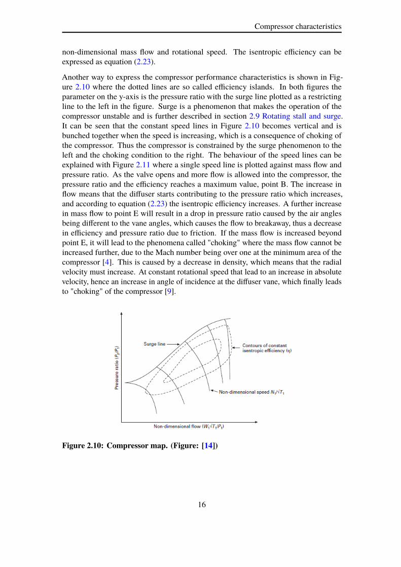
Another way to express the compressor performance characteristics is shown in Fig-ure 2.10 where the dotted lines are so called efficiency islands. In both figures theparameter on the y-axis is the pressure ratio with the surge line plotted as a restrictingline to the left in the figure. Surge is a phenomenon that makes the operation of thecompressor unstable and is further described in section 2.9 Rotating stall and surge.It can be seen that the constant speed lines in Figure 2.10 becomes vertical and isbunched together when the speed is increasing, which is a consequence of choking ofthe compressor. Thus the compressor is constrained by the surge phenomenon to theleft and the choking condition to the right. The behaviour of the speed lines can beexplained with Figure 2.11 where a single speed line is plotted against mass flow andpressure ratio. As the valve opens and more flow is allowed into the compressor, thepressure ratio and the efficiency reaches a maximum value, point B. The increase inflow means that the diffuser starts contributing to the pressure ratio which increases,and according to equation (2.23) the isentropic efficiency increases. A further increasein mass flow to point E will result in a drop in pressure ratio caused by the air anglesbeing different to the vane angles, which causes the flow to breakaway, thus a decreasein efficiency and pressure ratio due to friction. If the mass flow is increased beyondpoint E, it will lead to the phenomena called "choking" where the mass flow cannot beincreased further, due to the Mach number being over one at the minimum area of thecompressor [4]. This is caused by a decrease in density, which means that the radialvelocity must increase. At constant rotational speed that lead to an increase in absolutevelocity, hence an increase in angle of incidence at the diffuser vane, which finally leadsto "choking" of the compressor [9].

Figure 2.10: Compressor map. (Figure: [14])

16

2. THEORY

Figure 2.11: Plot of one speed line.

2.9 Rotating stall and surge

When the compressor is driven at a fixed speed, the flow is steady and there are smalldeviations in pressure and velocity. There are nevertheless circumstances that will makethe flow profile very unstable and unpredictable. Two phenomena that will cause thisare called rotating stall and surge [15]. Let us start with describing how rotating stall isinitiated.

As [14] writes, reduced mass flow gives an increased rotor inlet air angle. This can causeflow separating as it passes over blades, see Figure 2.12. Part of the flow that was meantfor channel C, goes through channel B instead and forces channel B to stall. This patternmoves along the impeller and rotates, relative to the rotor, in opposite direction withapproximately half the speed of the rotor, initiating rotating stall [14]. The phenomenacauses large vibratory stresses in the blading of the compressor and can lead to high bladestress levels [15]. Rotating stall decreases the efficiency of the stage, but the compressorcan in some cases still be able to perform. A danger with rotating stall is that it can leadto surge, which has negative effect on both the performance and the mechanical parts ofthe compressor [14].

Figure 2.12: This figure shows how air is pushed over channels, and can introducerotating stall. (Figure: [14])

17

Polytropic efficiency using the sT-method

Suppose the mass flow by any reason is reduced and rotating stall is initialized. The stalldevelops circularly and finally covers the whole flow annulus. This causes a significantreduction in efficiency and the compressor is no longer able to perform the requiredpressure rise. Because of the higher back pressure of the compressor the flow will bereversed and start to go backwards. The reversed flow will lower the downstream pressureand at some point the flow will return to its normal flow direction. Nevertheless, if theconditions that first initialized surge remains, the surge can re-occur. This change of flowdirection can occur with a high frequency and be very destructive for the compressor [14].The high pressure gradients contributes to high temperature gradients which has anadverse effect on the blade life expectancy [16].

2.10 Polytropic efficiency using the sT-method

In simple calculations the efficiency is calculated for the turbine or compressor as awhole. In fact this may lead to misleading calculation results when performing cyclecalculations. As can be seen in Figure 2.8 the isobars diverge as entropy increases. Thisresults in that the vertical distance between pressure lines (= temperature rise in eachinterval) differ throughout the process. As the efficiency depends on temperature risethe difference will increase with the number of stages in the compressor. To handle thisdifferently another efficiency is used, the polytropic efficiency. The polytropic efficiencyis defined as the isentropic efficiency of an infinitesimal small stage in the process, whichis a more accurate definition than the isentropic efficiency of the whole compressor [9].

As [17] writes, the polytropic efficiency is normally calculated with equation (2.27). Noderivation of this equation will be given here, hence it can be further studied in [17].

1 −(

p2p1

) γ−1ηpol ·γ

=1 −

(p2p1

) γ−1γ

ηis(2.27)

Equation (2.27) assumes that the gas is an ideal gas with constant cp. In performanceprograms that are used in this project the gas is handled as an semi ideal gas with a cpthat depends on temperature but not pressure. Due to this issue it would be advantageousto calculate the polytropic efficiency in a more accurate way. The sT-method is presentedby [17] and is the one used in this project. In this method the entropy is used, and notthe pressure as above. The efficiency is calculated with equation (2.28), with definitionsaccording to Figure 2.13. sT is the entropy for the outlet temperature at inlet pressure.

ηpol =sT − s2sT − s1

(2.28)

18

2. THEORY

T

S S

𝑝2

𝑝1

Figure 2.13: Definition of parameters for the sT-method.

2.11 Gas turbine

The gas turbine is a powerful and efficient power source. It transforms the energy in liquidor gaseous fuels into mechanical work. Historically the aerospace engines have beenthe leaders in this technology, due to the hard demands on the engines. They have to bedurable for high performance, high reliability and last for many start-up sequences. In the1990s the aero-derivative gas turbines were introduced, which improved the performanceof industrial gas turbines. In early 1950s the efficiency was around 15 %, but today it canbe as high as 45-50 %. Industrial gas turbines were between 1960s and 1980s mainlyused for peak-load, but as technology developed it became a great competitor againstother power sources, even at base-load [4].

Figure 2.14 shows the working principle of a single-shafted gas turbine. The medium isfirst flowing through the compressor were the energy from the shaft increase the pressureof the medium. The medium is then heated in the burner, where fuel is injected to increasethe temperature. In the turbine the pressure and temperature energy is transformed intorotational energy. Some of the energy is absorbed by the compressor and the excessenergy is used by the load through a mechanical shaft. The four thermodynamic stagesin the process are defined in the ideal Brayton cycle which can be seen in Figure 2.15.The numbers 1-4 represent the different components of the gas turbine. The two (ideal)isobaric processes represent the combustor and cooler, the isentropic represent thecompressor and turbine. In the general model there is no cooler for the outlet flow,instead this is represented by the ambient environment [4].

If a single-shaft gas turbine is used for MD there is often a need to unload the drivencomponent during start-up to reduce the torque needed [6]. A multi-shaft turbine has theadvantage that the gas generator and power turbine are not connected with a shaft andthereby are able to rotate with different speeds. This makes it easier to start the turbine

19

Gas turbine

with the driven load connected [18].

Feed

Load Compressor

Drain

Turbine

Combustor

1

2 3

4

Fuel input

Figure 2.14: Gas turbine working principle.

P

V

T

S

1

2 3

4 1

2 4

3

Figure 2.15: The Brayton cycle.

As seen in Figure 2.14 this gas turbine only have one shaft. Though, gas turbines can bedivided into two different groups, single-shafted and multi-shafted gas turbines. Theworking principle of a multi-shafted gas turbine is similar to a single-shafted, with thenatural difference that there is more than one shaft, see Figure 2.16. The single-shaftgas turbine is often used in purpose of PG, while the multi-shaft could be used for bothPG and in MD applications. In a multi-shaft gas turbine one shaft is connected to thecompressor and one to the load which allows the two shafts to rotate at different speeds.The multi-shaft cycle has advantages when it comes to part load and load variationsdue to its high torque at low rotational speeds, which is why they often appear in MDapplications [4].

20

2. THEORY

Feed

Load Compressor

Drain

Tu

rbin

e

Combustor

Fuel input

Tu

rbin

e

Figure 2.16: Gas turbine working principle, two-shafted.

2.12 Heat transfer

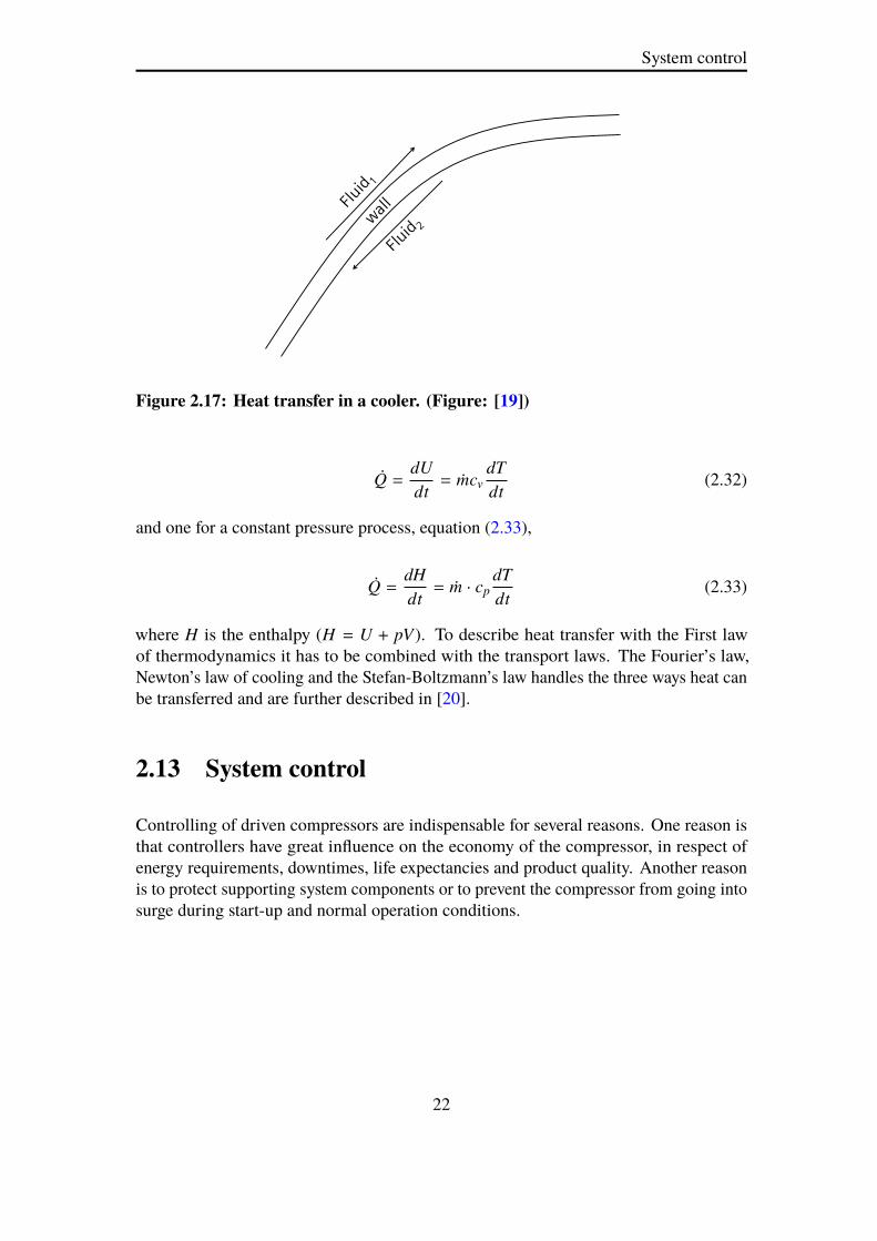
The concept of heat transfer is described in [19] as energy being transferred from thehot to the cold part of a substance, or from a body with a higher temperature to a bodywith a lower temperature. The bodies do not have to be in touch with each other, thougha temperature difference has to exist for the heat transfer to take place. Heat can betransferred in three ways: conduction, convection and radiation. The principle of heattransfer in a cooler, or heat-exchanger, is shown in Figure 2.17.

The heat transfer in a cooler can be written as equation (2.29)

ÛQ = HTC · A · ∆Tm (2.29)

where HTC is the overall heat transfer coefficient, A the area over which heat transferoccurs and Tm the mean temperature difference. Two ways to analyse a heat exchanger isthe LMTD-method and the ε-NTU method which are further described in [19]. Equation(2.30) states the first law of thermodynamics for a closed system.

ÛQ = Wk +dUdt

(2.30)

where ÛQ is the heat transfer rate, W k is the work transfer rate and the derivative dU/dtis the rate of change of internal energy. In a cooler where no work is done except pdVthe transforms into equation (2.31).

ÛQ = pdVdt+

dUdt. (2.31)

Equation (2.31) has two cases, one for a constant volume process, equation (2.32),

21

System control

Figure 2.17: Heat transfer in a cooler. (Figure: [19])

ÛQ = dUdt= Ûmcv

dTdt

(2.32)

and one for a constant pressure process, equation (2.33),

ÛQ = dHdt= Ûm · cp

dTdt

(2.33)

where H is the enthalpy (H = U + pV). To describe heat transfer with the First lawof thermodynamics it has to be combined with the transport laws. The Fourier’s law,Newton’s law of cooling and the Stefan-Boltzmann’s law handles the three ways heat canbe transferred and are further described in [20].

2.13 System control

Controlling of driven compressors are indispensable for several reasons. One reason isthat controllers have great influence on the economy of the compressor, in respect ofenergy requirements, downtimes, life expectancies and product quality. Another reasonis to protect supporting system components or to prevent the compressor from going intosurge during start-up and normal operation conditions.

22

2. THEORY

2.13.1 Anti-surge control

As mentioned above, surge is an undesirable phenomena, why recycle valves often areused. The recycle valve redirects some of the flow at the outlet of the compressor to theinlet in order to keep the flow through the compressor above the surge limit. Because ofrapid changes in system parameters safety measures are required and a control line isoften used. The control line is normally stipulated at a distance of 5-10 % to the rightof the surge line, i.e at 5-10% higher than the surge mass flow for a constant rotationalspeed. When the control line is reached, the recycle valve (see Figure 2.1) opens and theoperating point is moved away from surge. The surge margin can be calculated as (2.34)

SM =Ûmop − Ûms

Ûms(2.34)

where Ûmop and Ûms is the mass flow at the operating point and the mass flow on the surgeline respectively. For calculating with volume flow, Ûm is simply replaced with ÛV . Thedisadvantage of having a recycle line is the fact that the natural gas has to go through thecompressor several times, which increase the energy consumed by the compressor, thus,decreases the efficiency. Though the recycle valve can be seen as economical comparedto the damages that could arise [21].

2.13.2 PID-controller

A very common controller in the process industry is the PID-controller. The PID-controller works as a control loop feedback mechanism and has the ability to eliminateoffsets through integral action and to predict the future through derivative action. Theprinciple of a feedback controller is shown in Figure 2.18. The feedback of this typeis normally called negative feedback where y represents the operating value, ysp theset-point value, e = ysp − y the control error and u the control variable in the figure.When an error is present in the controller loop, it has to be eliminated in the best manner.One way in achieving this is the use of a PID-controller. The PID-algorithm can bedescribed as equation (2.35),

u(t) = K(e(t) + 1

Ti

∫ b

ae(τ) dτ + Td

de(t)dt

)(2.35)

where the three terms represents the P-term, the I-term and the D-term respectively. TheP-term is proportional to the error, the I-term is proportion to the integral of the errorand the D-term proportional to the derivative of the error. K is the proportional gain, Tithe integral time, Td the derivative time, t is the time and τ is the variable of integration.The PID-algorithm can also be represented by the transfer function (2.36).

23

System control

G(s) = K(1 +

1sTi+ sTd

)(2.36)

Σ Controller Process 𝑒 𝑢 𝑦𝑠𝑝

−1

𝑦

Figure 2.18: Block diagram of a simple feedback mechanism.

The simplest form of the PID-controller is the P-only controller which reduces equation(2.35) to equaton (2.37).

u(t) = Ke(t) + ub. (2.37)

The control action of the P-only controller is proportional to the error. When the controlerror is zero the control variable, u(t), becomes equal to ub(the bias or reset), which ischosen in a way so that the control error is zero at a given set-point or as a fixed value of(umax − umin)/2. A high value of K gives a faster control and a smaller control error, butwith the possibility of instability in the system which is illustrated in Figure 2.19.

If it is necessary to eliminate the error completely, the addition of the integral term isneeded, which gives us the PI-controller. The integral term assures that the process outputagrees with the set-point due to the integration of the error over time. The PI-controlleris described by equation (2.38)

u(t) = K(e(t) + 1Ti

∫ b

ae(τ) dτ). (2.38)

For large values of Ti the response of the system is slower in approaching the set-point,but with less oscillations and instability which can be seen in Figure 2.20.

24

2. THEORY

Figure 2.19: The upper diagram shows the set-point, ysp = 1, and the processoutput, y. The lower diagram shows the control signal u for differentgain values, K . (Figure: [22])

Figure 2.20: The upper diagram shows the set-point, ysp = 1, and the processoutput, y. The lower diagram shows the control signal u for differentintegral times, Ti, with K = 1. (Figure: [22])

The derivative part can be added to improve the stability of the closed loop, whichmakes the PID-controller complete and forms equation (2.35). With the use of thederivative of the error the controller predicts the behaviour of the error and will be ableto respond more quickly than a controller without derivative action. Different valuesof the derivative time, Td is shown in Figure 2.21, where the larger Td value dampensthe oscillations at first but further increasing of Td decreases the damping. For mostprocesses the PID-controller is sufficient and a more complex controller is not needed. Aproblem that follows with the PID-controller is the tuning of the parameters. This can bedone in several ways, for example with the Ziegler-Nichols methods [22].

2.14 Start-up sequence

As stated by [4], the start-up sequence is one of the major functions of a control system.Normally the start-up sequence is in charge of the operation up to 50 % of the maximumrotating speed. In the compressor train simulated in this project there is one controller

25

Purge

Figure 2.21: The upper diagram shows the set-point, ysp = 1, and the processoutput, y. The lower diagram shows the control signal u for differentderivative times, Td , with K = 3 and Ti = 2. (Figure: [22])

for the compressor and one for the gas turbine, and they have different tasks duringstart-up. How the start sequence is designed depends on many factors such as compressormanufacturer, model and if it is driven by a gas turbine or electrical engine [4].

If a compressor system is equipped with an anti-surge loop the valve is normally fullyopen during start-up, as mentioned. The mechanisms that control the inlet flow, as guidevanes or inlet throttles, are in their minimum position to keep a low inlet flow. This isdue to the low torque at low rotational speeds. The anti-surge loop strives to have a highmass flow through the compressor. When the start-up procedure is finished the anti-surgevalve closes and another control system takes over the operation of the system [21].

The gas turbine has in turn its own start-up sequence, designed according to firingtemperature, torque at low speeds and many other parameters [4]. How the sequence isdesigned depends on the configuration, if it is a single- or multi-shafted turbine and ifit is a PG or MD application. An electrical starter engine is used from stationary to acertain speed level, and the power of this engine may vary a lot. Power requirements for a150 MW gas turbine can be as high as 5 MW, and for a gas turbine of 30 MW with a freepower turbine the requirements can be as small as 20 kW. The power requirements for agas turbine with free power turbine is always less than for a single-shafted, because the gasgenerator being the only part being accelerated and not the whole rotor [9]. The controlsystem that controls the start-up sequence till be further described in chapter 3.3 Dymolamodel of gas turbine control system.

2.15 Purge

In the gas turbine there are explosive fluids, as the fuel, which can cause fatal damages ifburning or exploding at the wrong time and wrong place. Before start these fuels canexist in shape of liquid or vapour in places where it is not supposed to be. To solve thisproblem the gas turbine is purged with ambient air before start. The purge process can

26

2. THEORY

for example be designed according to the National Fire Protection Association (NFPA)85: Boiler and Combustion Systems Hazards Code (2011), which is a code that sets”design, installation, operation, maintenance, and training” standards for ”safe equipmentoperation” [23].

In NFPA 85 some requirements are stated. The purge shall for example be at least fivevolume changes and last for more than five minutes. Also, the mass flow during purgehave to be at least 8 % of full power mass flow [23]. The purge time is calculated withequation (2.39) [24]. NFPA 85 is an American standard and the purge values can bechanged depending on the site. When modelling in Dymola the purge speed level, timeand other parameters can be set manually.

tpurge = np ·(

VGTÛVpurgeGT

+VE xsys

ÛVpurgeE xsys

)(2.39)

2.16 Natural gas

Natural gas is a fossil fuel that was produced by nature millions of years ago. Just as coaland oil it consists of remains of plants and animals that have been transformed becauseof pressure and heat in layers deep down in the ground. The gas often occurs in naturalpores in the bedrock and in coal deposits, which is called coal bed methane [25].

The natural gas contains mainly of methane (80 to 95 %), and small amounts of ethaneand other hydrocarbons [26]. When analysing natural gas it is often defined as a dry gas,but in reality the gas is never free from liquids. Water condensate in the pipeline andliquids from the lubrication systems in pumping stations makes it a wet gas [4].

Transportation of natural gas is a great challenge. The gas is transported from producingareas to areas with high demand. The efficient and effective way to do this is withpipelines. The network of pipelines worldwide is huge and can cross whole countries,for example east-west pipeline in USA and Russia. Pump stations are placed in thesenetworks to give the gas the pressure needed for transportation [27].

2.17 El-Encino

The El-Encino project is an ongoing Siemens project still under construction and it isused as a reference project in this thesis for verification and evaluation purposes. The siteis located in Mexico and will be a part of the "La Laguna" pipeline that will run a totalof 465 km between El-Encino and La Laguna. The compressor station, that Siemens hasa vital role in constructing, will have three parallel compressor trains consisting of the

27

Tools

SGT-750 as the driving component and the STC-SV as the driven component. In thisthesis the data used in the compressor system verification is retrieved from El-Encino.

2.17.1 SGT-750

The SGT-750 is an industrial gas turbine with the weight advantages of an aero-derivativegas turbine and the robustness and flexibility of an industrial gas turbine. It wasdesigned for long operating times and is easy to maintain and with a high availabilityand reliability. Because of the low downtimes for planned overhaul and maintenance theSGT-750 achieves a high availability which makes it useful both for PG but especiallyfor MD purposes. SGT-750 is a twin-shaft axial gas turbine with a two stage free powerturbine which delivers 41 MW in MD applications. The gas generator consists of anaxial compressor with 13-stages and an overall pressure ratio of 24.3. The gas turbinecompressor is driven by a two staged turbine which consists of an inlet stator with guidevanes where the first stage is cooled by both convective and film cooling. The SGT-750has an efficiency of 40.3% for PG and 41.6 in MD applications and is suitable for bothliquid and gaseous fuels [28].

2.17.2 STC-SV

The compressor used in the El-Encino project is a compressor of the STC-SV series.The compressor is a single shafted centrifugal compressor with vertically split casingand there could be up to ten impellers in a single casing. The STC-SV is a diversifiedcompressor that can be used in both standard and high-pressure applications. With itsrobust design it allows high nozzle loads and compression of gases with any molecularweight. The STC-SV is optimized for applications with low molecular weight and highpressure [29].

2.18 Tools

2.18.1 Dymola

The main software used in this report is the simulation and modeling tool Dymola,DynamicModeling Laboratory, which makes it possible to handle complex and integrateddynamic systems. The software is based on the Modelica language which is an object-oriented, declarative, multi-domain modeling language. Modelica uses equations todescribe physical systems instead of algorithms which makes it easy to use and tounderstand. When the governing equations have been stated for a system, Dymolatranslates the equations into a code. Dymola has two modes in terms of modelling, the

28

2. THEORY

text or code editor, and the graphical editor. The graphical editor in Dymola is a dragand drop editor in which it is possible to connect different parts into complex systemswhich is a convenient way to create models without having any deeper knowledge in theModelica language. Dymola and the Modelica language offers the possibility to createnew models from scratch, but also, there is the option of modifying existing models intothe system by adding new code or new components to it. Except for the two modelingmodes mentioned, Dymola also consists of a simulation mode. In the simulation modethe equations are solved and the user has the possibility to visualize the system by plottingthe dynamic behaviour [30].

2.18.2 SVN/GITLab

SVN and GITLab are two version management systems used at Siemens where updatedDymola models are checked in and made available for all employees. The system isglobal which make the models available from Siemens sites all over the world.

2.18.3 STA-RMS

STA-RMS (Siemens Turbomachinery Applications - Remote Monioring System) isa database consisting of raw data retrieved from all Siemens sites around the world.In RMS-View the user can study and download performance data from as late as theprevious day for any machine active on site. The STA-RMS is used in this thesis toretrieve data for MD sites in order to verify the behaviour of the compressor train model.

2.18.4 WebPlotDigitizer

WebPlotDigitizer is a tool used to extract numerical data out of plots and images. Thetool can handle different kinds of 2-D plots and allows the user to calibrate the axes andthen choose the points of interest in the plot. The data can then be exported to Excel forfurther use.

2.18.5 VLE Flash

VLE Flash is a tool developed for the natural gas & petroleum industry by Flow Phase Inc.The tool calculates thermodynamic properties and draws phase envelopes and vapourfraction lines of different fluid mixtures which can be exported to Excel. The programconsists of a database of 215 components, mostly hydrocarbons, and mixtures of up to20 components can be studied [31].

29

3. Methodology

This section treats the different steps that have been carried out during the project. Itprovides information of how the compressor model was constructed and includes theassumptions and decisions that were made when modelling different components.

The first step of the project was to perform a literature study where reports and articleswere reviewed. From this study the chapter Theory were created. The literature study isrepresented in the theory section. Equations and methods on how a compressor systemcould be modelled were found in the literature and created a base for the compressormodel and auxiliary systems. The compressor system was modelled in Dymola part bypart in order to ensure stability of the system. When the model fulfilled the specificationsand requirements needed, the model was implemented by connecting it to the existingDymola model of the SGT-750.

3.1 Literature study

During the first steps of the literature study available literature were reviewed andcategorized according to topic and relevance. The literature was both internal withinSiemens and external. The categorizing system made it easy to retrieve literature later inthe project and find information about a specific topic. By doing this the literature studywere performed continuously during the project as new components were modelled.

The literature study gave basic knowledge related to the project, such as governingequations and information about auxiliary systems as valves and control systems. Bylooking at similar projects the set-up for the simulation could be optimized to give thebest result.

31

Dymola model of compressor system

3.2 Dymola model of compressor system

During the years SIT engineers have designed their own Dymola Model Library,containing several basic models that can be used in more complex systems. Theserepresent a variety of components and are specially designed to fit the company’sapplications well. Some examples of modelled components are valves, pipes andcompressors. When designing the compressor train in this project these basic modelsoften represent a platform to start from, even though many components are designedfrom scratch.

The compressor system was modelled as the first part of this project and consists of anumber of components, which can be seen in Figure 3.1 below. The components will bedescribed further in the following sections.

Figure 3.1: The compressor system modelled in Dymola.

3.2.1 Compressor

The compressor modelled in this thesis is based upon the existing basic compressormodel developed by Siemens, with features rebuilt for the specific application. Thissection describes how the basic model is constructed and how it has been adjusted in thisthesis.

32

3. METHODOLOGY

3.2.1.1 Basic Model

The basic model developed by Siemens is a thermodynamic compressor model based oncharacteristics. The model uses three governing equations to describe the behaviour ofthe compressor, the energy balance, the mass balance and the substance mass balance.These can be written as equation (3.1), (3.2) and (3.3) respectively.

Ein − Eout = ∆Esystem (3.1)

Ûmin − Ûmout = ∆ Ûmsystem (3.2)

ÛmXi,in − ÛmXi,out = ∆ ÛmXi,system (3.3)

The process is assumed in the model to be adiabatic, continuous and with constant massfractions which changes the above equations to:

Win + Ûm(∆h) = 0 (3.4)

Ûmin − Ûmout = 0 (3.5)

ÛmXi,in − ÛmXi,out = 0. (3.6)

To calculate variables of interest the basic model make use of control volumes describedin section 2.2 Compressor. It also uses the ideal gas model according to 2.5 Ideal gasmodel. The medium in the model consists of different substances and retrieves baseproperties as enthalpy, entropy, inner energy and molar mass by using the ideal gas databased on NASA Glenn coefficients. It is a library containing thermodynamic data forover 2000 solid, liquid and gaseous species for temperatures between 200 and 20000K. The NASA Glenn coefficients will not be further described in this thesis but can bestudied in [32].

3.2.1.2 Characteristics

The compressor characteristics implemented in the model differs from the characteristicsdescribed in 2.8Compressor characteristics. The characteristics is visualized in Figure 3.2,where the x-axis is standard volume flow, the y-axis is discharge pressure and instead ofisentropic efficiency the discharge temperature is plotted in the characteristics as the blue

33

Dymola model of compressor system

lines. The normalized speed is still the fixed parameter as described in 2.8 Compressorcharacteristics. A single map covers only the performance at a specific compressor inletpressure. In MD applications the inlet pressure to a compressor train varies which iswhy two maps as the one in Figure 3.2 for different inlet pressures were implemented inthe model to increase the accuracy.

Volume flow [ [MMSCFD60F]

Guar. ControllinePower Requir.PiDischarge Temperature

105.0 %100.0 %

90.0 %

80.0 %

70.0 %

60.0 %

50.0 %

Out

let P

ress

ure

[psi

A]

Figure 3.2: The compressor characteristics used in the model. The volume flowgiven in MMSCFD60F (million standard cubic feet per day at 60Fahrenheit and 1 bar) and the pressure in PsiA. The straight lines rep-resent the power needed and the dotted ones represent the dischargetemperature.

The compressor maps were added to the model through reading of the values in the actualmap, due to values not being available in table form. The pressure and volume flowwere added with the program WebPlotDigitizer and the temperatures were estimated byhand. Since the compressor maps are created down to 50% of nominal speed the lowerspeeds had to be extended by hand and manually put in to the Dymola code. The mapsare used in the model as a sequence of inter- and extrapolation depending on the actualconditions. These are performed in 3D between different inlet pressure maps, in 2Dbetween speed lines and in 1D on the actual speed line. Inputs to the characteristics areinlet pressure, rotational speed and discharge pressure. The outputs are volume flow,surge factor and discharge temperature, which can be seen in Figure 3.3 below. Thevolume flow is converted to mass flow in the model with a reference density at pressure

34

3. METHODOLOGY

and temperature of 1 bar and 60 F. The Variable Guide Vane input to the compressormap is not used in this project due to limitations, however it is still in the model due tothe fact that it could be used in future models at Siemens.

Figure 3.3: The Dymola model of the compressor.

3.2.2 Medium

The medium in the compressor model in Dymola was created according to the naturalgas specified in the El-Encino project. The gas composition can be seen in Table 3.1.

3.2.3 Compressibility

In this report the medium to compress was natural gas, that mainly consist of methane.The parameters for methane is given in Table 3.2. In this report the pressure is in therange [50, 80] bar and [289, 373] K, which gives a pR in the range of [1.09, 1.74]and TR in the range of [1.51, 1.95]. By using Figure 2.5 it can be found that the fourcombinations of pR and TR gives a Z of Z1 = 0.9, Z2 = 0.97, Z3 = 0.85 and Z4 = 0.95.That means that in the worst case scenario Z = 0.85. In the modelling it only affects thecalculation of density and inner energy, but does not change the value of the referencemedium when converting between units (from MMSCFD60F to kg s−1). The referencemedium has a pressure of 1 bar and temperature of 60 F which gives Z = 1. The resultof this is that Z will not affect the calculations or result in a significant way. In the

35

Dymola model of compressor system

Table 3.1: Composition of the Natural Gas in the model.

Substance M [kg/kmol] Mol%

Methane 16.04 93.665

Oxygen 32.00 0.149

Carbondioxide 44.01 0.955

Nitrogen 28.02 0.149

Water 18.02 0

Ethane 30.07 4.815

Propane 44.09 0.218

n-Butane 58.12 0.02

Isobutane 58.12 0.021

n-Pentane 72.15 0.002

Isopentane 72.15 0.003

n-Hexane 86.17 0.003

original Dymola functions the gas is handled as an ideal gas with a compressibility factorequal to 1. Due to that, the Z-value was added as a parameter in the compressor and inthe medium for future development of the model.

Table 3.2: Equations for gas properties. Table: [12]

Substance M [kg/kmol] R [kJ/kgK] pR [MPa] TR [K]

Methane, CH4 16.04 0.518 4.6 191

3.2.4 Anti-surge loop

The compressor system in this project is equipped with an anti-surge loop. This loopconsists of a control valve that is controlled by a control system. The purpose of theloop is to avoid surge in the compressor, and its components are further described infollowing sections.

3.2.4.1 Control valve

The anti-surge valve is one of two valves used in the compressor model in order to controlthe flow. The characteristic of the valve was set as linear which means that 10 % openinggives a 10 % flow of maximum [12]. The valve was designed according to specificationsof the El-Encino project and have a Kv value of 1650. The Kv is known as the flow

36

3. METHODOLOGY

coefficient and states the number of cubic meters of water flowing through the valve perhour, with a pressure loss of one bar. The opening and closing of the valve is controlledby an input signal from the control system described below.

3.2.4.2 Control system

The anti-surge control system is used to control the operation of the anti-surge controlvalve. When opening the control valve the flow is redirected to the inlet of the compressor,and the mass flow through it increases. The system can be seen in Figure 3.4. It consistsof a PI-controller that responds to the surge margin, calculated according to equation(2.34), and the set point which is the surge limit chosen by the user. The controllerwas modelled to cover two main operating cases, start-up and normal operation. Thecompressor speed, normalized to the nominal speed (6100 rpm), is used as an input tothe controller to cover the start-up case where the anti-surge valve is fully open. Duringnormal operation the control system switches to the PI-controller when the minimumcontinuous speed is reached, which is the speed where the gas turbine can operate anddrive the load on its own. In order to avoid unstable behaviour a hysteresis was added tothe controller and a ramper was added to control the opening and closing time of thevalve.

Figure 3.4: The Dymola model of the anti-surge loop control system.

37

Dymola model of compressor system

3.2.5 Check valve

A check valve was modelled at the outlet to prevent reversed flow from the downstreampipeline. An example of a check valve is the swing valve, as can be seen in Figure 3.5.Unlike the control valve the check valve is either totally open or totally closed and do nothave to be controlled in the same extent as the control valve, thus no control system ismodelled for this component. Despite this, all types of check valves acts differently andthey all got unique characteristics [12].

Figure 3.5: Swing check valve. (Figure: [33])

3.2.6 Cooler

According to equation (2.23) the pressure rise contributes to a temperature rise of themedium. Because of the surrounding circumstances it is required to maintain a lowtemperature of the medium, 16 C. This applies to the outlet of the system, but also to theanti-surge loop. During start-up the recycling valve will be open, and without a coolerthe temperature in the loop would increase successively. For this reason the cooler wasplaced after the compressor.

The task of a standard cooler is to exchange heat between mediums. Figure 3.6 showsan example of a cooler, a Shell-and-Tube heat exchanger. One fluid is passing in thetubes, one in the surrounding shell and heat is transferred between them. The largertemperature difference and heat transfer area in the exchanger, the larger amount of heatis transferred [12]. However, the heat exchanger in this project was not modelled as astandard heat exchanger. Instead it was modelled as a simplification where the outlettemperature was set to 16 C and the transferred heat flow, ÛQ, was added to the energybalance according to equation (3.7). By doing this the heat exchanger does not need anycold medium or any controlling of the cooler outlet temperature.

Ûm(∆h) − ÛQ = 0 (3.7)

38

3. METHODOLOGY

Figure 3.6: Example of a Shell-and-Tube heat exchanger. (Figure: [34])

3.2.7 Source, Sink and Volumes

A source and a sink were also added in the model. They represent the upstream anddownstream of the pipeline and can be seen as an infinitely large volume containingnatural gas. In order for the system to be dynamic volumes had to be added as well.The values of the volumes were set according to the El-Encino case and represent thevolumes of piping between components, and the components themselves.

3.2.8 Ideal gas model

When the verification of the compressor system was performed it was noticed thatDymola only handles ideal gases, therefore an investigation of how this affects theaccuracy of the model were performed. The main issue were the inaccurate enthalpycalculation performed by Dymola. It was investigated if Dymola only calculates theenthalpy with respect to temperature. The enthalpy for the main substance, Methaneat 48 C, was retrieved from [35] and compared with the enthalpy from Dymola. Thesoftware VLE Flash was used to calculate the enthalpy for natural gas treated as a realgas at the same operation points as in the verification of the compressor system.

3.3 Dymola model of gas turbine control system

To be able to run a gas turbine in a correct manner, all turbines are equipped with acontrol system. This system has three fundamental functions: start-up and shutdownsequencing, steady-state control during operation and protection of the gas turbine [4].When using a gas turbine in an MD application instead of a PG application the controlsystem had to be modified. In general the control system looks the same, but somecomponents were added or replaced. This will be further described in the respective

39

Dymola model of gas turbine control system

section. Unless the opposite is stated, the controller works in the same way for bothapplications.

There are two main types of control systems - closed or open loop system. The opensystem induces a control signal for the system without any measurements. The closedsystem is controlled with a measured signal from the system itself. By calculatingthe deviation between the measured signal and a set point, the control signal can bechanged [4].

The control system for the SGT-750 mainly consists of closed loops and contains manycontrollers who together control different parameters and values of the gas turbine. Theyall have their own tasks and limits, for example one controller controls the gas generatorspeed which has a maximum value and another controls the speed of the power turbine.The controllers are activated automatically when they are closest to its limit and thenassume control of the operation. In the SGT-750 control system there are many differentcontrollers, but in this report only the ones that are vital for this project are mentioned.Figure 3.7 shows a graphic view of the controllers in Dymola. The three controllers inthe MD box were the ones modelled in this project and during MD operation the FLCcontroller was deactivated to ensure the right control of the gas turbine.

Figure 3.7: The modelled control system for SGT-750. The controllers in the greenbox are specially designed for MD applications.

40

3. METHODOLOGY

3.3.1 Starter motor

The starter motor has two main purposes: to drive the gas turbine through a purge processand to accelerate the gas generator up to a speed where it got enough mass flow to provideitself with power. The starter motor is an electrical engine and its size depends on thetype and size of gas turbine.

3.3.2 Start controller - STC

The start controller is the first controller to take over from the starter motor duringstart-up. When chosen rotational speed is reached the STC starts the ignition and thenactivates a fuel ramp to the burner which causes the firing temperature to rise and thegas generator to accelerate. The purpose of the STC is to get good starting reliability andto avoid engine damage. By limiting the rotor acceleration, the STC prevents too highthermal stress of the turbine. The STC is active until the gas generator reaches a certainspeed, around half way through the acceleration, where NGGL takes over the operation,see section 3.3.3 Gas generator speed limiter - NGGL [24].

3.3.3 Gas generator speed limiter - NGGL

When the NGGL is in operation it uses a PID-controller to accelerate the gas generatorwith a constant ramp. The value of the ramp changes at a certain speed. The controllerlimits the gas generator speed to avoid engine damage. For a PG application the NGGLis active until operation speed is reached, which is when the generator has the samefrequency as the grid (50 Hz in Sweden). Though, for an MD application NGGL isactive until just before min. continuous speed is reached, which depends on the operationsituation [24].

3.3.4 Power turbine acceleration controller - PAC

This was the first controller modelled in this project. For an MD application it ismore important to have a PAC which limits the acceleration of the PT, because of itslower inertia. A too high acceleration can damage the power turbine. The feedback forPID-controller in the PAC is the derivative of the PT speed, which is limited to a givenvalue [24]. If the PAC is active it gives the power turbine speed this constant derivative.The PAC is active during start-up and up to a set point close to the min. continuousspeed, just as NGGL. This means that PAC is active at the same time as both STC andNGGL. The design of the PAC can be seen in Figure 3.8.

41

Dymola model of gas turbine control system

Figure 3.8: Dymola design of PAC - power turbine acceleration controller

3.3.5 Frequency and load controller/Speed controller - FLC/SC

In PG applications the FLC is active until idle speed is reached during start-up. It canbe set to either frequency control or load control depending on the situation. In thisproject the FLC is inactive and replaced with the SC. The SC takes over from NGGL andPAC during start-up just before min. continuous speed. It uses a PID controller to keepthe PT speed at a required level. Even if the controller focus on the speed, the powerturbine acceleration is limited due to a table in [24]. This table give loading restrictionsin rpms−1 based on gas turbine compressor discharge pressure. The design of the SCcan be seen in Figure 3.9.

3.3.6 Mass flow controller - MFC

Even if the SC controls the PT speed (and thereby the speed of the driven component), itis not practical for the operator to control the gas turbine in such a way. That is why itoften is advantageous to add another controller. In this project it was desirable to controlthe system on mass flow through the driven compressor, which is why the MFC wasmodelled. The MFC uses a PID controller to control the PT speed by measuring thedeviation of the actual mass flow and the mass flow set point. The model was designedso that the user easily can deactivate the MFC controller and use the SC instead. Thedesign of the MFC can be seen in Figure 3.10.

42

3. METHODOLOGY

Figure 3.9: Dymola deisgn of SC - Speed controller

3.3.7 Exhaust temperature limiter - T0800L

At full load operation the T0800L controller limits the exhaust temperature, T0800.The purpose of this is to limit the turbine inlet temperature, TIT, due to materialcharacteristics [24]. The controller measures both TIT and T0800 and compares themwith their maximum values.

3.3.8 Load loss detection - LLD

The purpose of the LLD is to have a high sensibility when instant load drops occur. Ifone should occur the LLD reduces the fuel down to flame sustain level and opens thebleed valves according to a prescribed table [24]. This controller is not modified in thisproject.

43

Dymola model of gas turbine control system

Figure 3.10: Dymola deisgn of MFC - mass flow controller

3.3.9 Gas generator acceleration control - GAC

The GAC controls the upper limit of the fuel flow to avoid overheating and compressorsurge. The fuel flow limit is set by the actual normalized compressor speed [24]. Thiscontroller is not modified in this project.

3.3.10 Flame sustain control - FSC

This controller is very important and gives a lower limit of the fuel flow. This limit is thelowest possible flow to sustain the flame, though the other controllers can call for a fuelflow below this. In case of a flameout the flame has to be re-lit, which takes time and isbad for the performance [24]. This controller is not modified in this project.

3.3.11 Gas generator deceleration control - GDC

The GDC is also used to avoid flameout, it controls the minimum fuel flow based on thenormalized gas generator speed. The lower limit is also depending on PG or MD. Foran MD application the lower limit is increased with required fuel flow to match load atminimum PT speed [24]. This controller is not modified in this project.

44

3. METHODOLOGY

3.3.12 Bleed valve controller - BVC

The BVC controls the compressor bleeds, that are used to lead away some of the air in thegas turbine compressor. This is done to manage differences in stage compression causedby speed variations. This allows the compressor stage to operate at low speeds withoutstalling, because of choked subsequent stages [24]. This controller is not modified inthis project.

3.4 Implementation - Connecting the compressor sys-tem with the SGT-750

One of the main objectives in this project was to connect the compressor model withthe existing SGT-750 model at Siemens and then simulate a starting sequence. In orderto achieve this several changes had to be made in the SGT-750 model. The SGT-750model were previously built to simulate dynamic behaviour during PG and therefore hadto be adapted to the MD application. The compressor model and the modified SGT-750model can be seen in the Figure 3.11 below. The features including the frequency ofthe generator had to be changed to power turbine speed in order to be able to controlthe compressor train in a correct manner. New controllers were added to the SGT-750controller which has been described in the previous sections.

45

Implementation - Connecting the compressor system with the SGT-750

Figure 3.11: The SGT-750 system connected with the compressor system.

46

4. Verification and analysis

To be able to analyse the gas turbine behaviour in a MD application one have to ensurethat the thermodynamic model corresponds to reality. This is done with the verificationprocess presented in this chapter. The verification is visualized in normalized graphsdue to company secrecy. The graphs were normalized with the final or maximum valuefor the studied sequences. The verification was divided into two sections. Firstly theverification of the compressor model was performed, with data from the compressormanufacturer. Secondly, when the compressor system and the gas turbine were connectedinto a compressor train, the entire compressor train’s performance was verified in threesteps that will be further described in the current section.

4.1 Verification of the compressor system

As a part of the verification of the compressor system, simulations were performed attwo steady state operation points with the purpose of verifying the compressor. Thechosen points represent two scenarios from two different compressor maps, i.e. differentcompressor inlet pressures. The results of the simulations were compared with data sheetsfrom the compressor manufacturer. The deviation for each parameter was calculated withequation (4.1), where Xsimulation is the parameter value from the simulation and Xdata isthe given parameter value from the compressor manufacturer. The average deviation ofthe two scenarios was calculated with equation (4.2) where X1 is the deviation from onescenario and X2 from the other.

deviation =(

Xsimulation

Xdata− 1

)· 100 (4.1)

average deviation =X1 + X2

2(4.2)

Parameters that were compared with the data sheet were inlet volume flow, compressoroutlet temperature, polytropic efficiency, power and polytropic head. The volume flow

47

Verification of the compressor system

and temperature were retrieved in the model as outputs from the compressor map, thepolytropic efficiency was calculated according to 2.10 Polytropic efficiency using the sT-method, the power according to equation (4.3) and the polytropic head as equation (4.4).The polytropic head denotes the amount of work required per kilogram of compressedgas.

P = ∆h · Ûm (4.3)

Headpoly = Znaturalgas · Rinlet · Tinlet ·γinlet

γinlet − 1

(poutlet

pinlet

γinlet−1γinlet − 1

)(4.4)

The anti-surge loop was an important part to verify when verifying the compressorsystem. Focus were on the control system of the control valve, i.e. to ensure that the surgemargin were kept above the chosen limit and that the control system behaved as intended.Two different simulations were performed, a start-up and a steady state to verify bothcases mentioned in 3.2.4.2 Control system. During the verification the anti-surge loopcontrol system was tuned in, in order to keep a steady and accurate control of the surgemargin.

4.1.1 Compressor verification

To verify the compressor, the two steady state operational points mentioned in 4.1 Veri-fication of the compressor system, were simulated. The input data for the two scenarioscan be seen in Table 4.1, under ”Input”. The deviation for each parameter was calculatedwith equation (4.1), and the average deviation was calculated with equation (4.2). Theaverage deviations can be seen in Table 4.1 under ”Avg. dev.”.

Table 4.1: Verification results for the compressor system. ”2023” means ”Scenario1A, 2023, 1 train” and ”2024” means ”Scenario 1A, 2024, 1 train”. SI-units are not used since the data sheets from manufacturer were inAmerican units.

Input Output

Parameter 2023 2024 Parameter Avg. dev. [%]

Inlet pressure [psiA] 733.7 799.4 Inlet volume flow [MMSCFD60F] 0.1

Outlet pressure [psiA] 1025.2 1131.5 Comp. outlet T [C] 1.6

Comp. inlet T [C] 16 16 Polytropic efficiency [%] 2.8

Comp. rotational speed [rpm] 4643 4828 Power [kW] 15

Polytropic head [kJ kg−1] 0.7

48

4. VERIFICATION AND ANALYSIS

As can be seen in Table 4.1 the deviations in general can be considered small. Thepower has a larger deviation due to miscalculated enthalpy in Dymola. This phenomenais described in chapter 3.2.8 Ideal gas model. As mentioned, the temperature wasmanually put into the model, which contributes to the deviation of the compressor outlettemperature and the polytropic efficiency.

4.1.2 The ideal gas model

The result of the ideal gas model investigation can be seen in Figure 4.1 and in Table 4.2.In Figure 4.1 the blue line represents the enthalpy retrieved from [35] and the red linethe enthalpy calculated in Dymola for Methane. The enthalpies have different referencestates which causes a greater difference between the lines in the figure. It can be seenthat the enthalpy has a clear pressure dependency during circumstances with this highpressure. Table 4.2 shows that the average deviation of the power was decreased from 15% to 3.72 % when using the real enthalpy instead of the enthalpy from Dymola. Theenthalpies shown in the figure

550

650

750

850

950

1050

0 50 100 150 200 250 300

Enth

alpy [

kJ/

kg]

Pressure [bar]

Real enthalpy

Dymola

Figure 4.1: The figure shows the enthalpy retrieved from [35] and the enthalpyfrom Dymola for Methane as a function of pressure.

49

Verification of the compressor system

Table 4.2: Table showing the average deviation of the compressor power whenusing the enthalpy retrieved from VLE Flash for the two cases used inthe verification of the compressor system. SI-units are not used sincethe data sheets from manufacturer were in American units.

Case pcomp. inlet pcomp. outlet ∆h Dev Avg. dev

[psiA] [psiA] [kJ/kg] [%] [%]

2023 733.7 1025.2 63.75 3.743.72

2024 799.4 1131.5 67.90 3.71

4.1.3 Start-up

To verify the control system two different sequences were simulated, the first one was thestart-up sequence.

Figure 4.2 shows the compressor speed during the start-up sequence, starting from almostzero rpm up to nominal speed of the compressor.

0

0,2

0,4

0,6

0,8

1

1,2

0 50 100 150 200

Norm

aliz

ed r

ota

tional

spee

d

Time [s]

Figure 4.2: Compressor speed during start-up of the compressor system.

Figure 4.3 shows the opening level of the anti-surge valve during the start-up sequence.The valve follows the prescribed closing time according to [21].

50

4. VERIFICATION AND ANALYSIS

0

0,2

0,4

0,6

0,8

1

1,2

0 50 100 150 200

Val

ve

open

ing

Time [s]

Figure 4.3: Opening of the anti-surge valve during start-up of the compressorsystem.

Figure 4.4 shows how the surge margin varies during a starting sequence. As the speedstarts to increase the surge margin increases quite unevenly due to the inaccuracy ofthe map for speeds below the min. continuous speed. When this speed is reached thecontrol valve starts to close as can be seen in Figure 4.3, and the surge margin decreases.When reaching 10 % the PI-controller keeps the margin at this limit and as the speed stillincreasing it will increase the mass flow, thus increase the surge margin.

51

Verification of the compressor system

0

0,1

0,2

0,3

0,4

0,5

0,6

0,7

0,8

0,9

0 50 100 150 200

Surg

e m

argin

[%

/100]

Time [s]

Figure 4.4: Surge margin during start-up of the compressor system.

In Figure 4.5 the mass flow of the start-up sequence can be seen. As the speed increases,the mass flow increases. When reaching min. continuous speed the anti-surge valvecloses and the mass flow through the loop decreases. Since the pressure is still below theback pressure in the sink the mass flow in the loop is the same as through the compressor.As the valve closes entirely the outlet mass flow increases when the back pressure isreached.

52

4. VERIFICATION AND ANALYSIS

0

0,2

0,4

0,6

0,8

1

1,2

0 50 100 150 200

Norm

aliz

ed m

ass

flow

Time [s]

Loop

Outlet

Figure 4.5: Loop and outlet mass flow during start-up of the compressor system.

The pressure have a clear dependency of the opening of the anti-surge valve which canbe seen in Figure 4.6. As speed is increasing a small amount of pressure is building up,but as the valve closes pressure starts to build up rapidly. In order to reach a dischargepressure higher than the sink pressure the valve closes as much as it is allowed duringstart-up of the compressor system.

53

Verification of the compressor system

0,4

0,5

0,6

0,7

0,8

0,9

1

1,1

0 50 100 150 200

Norm

aliz

ed p

ress

ure

Time [s]

Compressor outlet

Sink

Figure 4.6: Outlet and sink pressure during start-up of the compressor system.

4.1.4 Steady state

A steady state case was simulated as a negative ramp of the rotational speed in order toverify that the anti-surge loop control system starts to act when the surge limit is reached.

Figure 4.7 shows the speed ramp for the steady-state simulation, going from full speeddown to 97.5 %.

54

4. VERIFICATION AND ANALYSIS

0,96

0,97

0,98

0,99

1

1,01

0 50 100 150 200

Rota

tional

spee

d [

rpm

]

Time [s]

Figure 4.7: Compressor speed during the steady state sequence.

Figure 4.8 shows the opening of the anti-surge valve during the steady state sequence.The control of the valve shows no indications of oscillations or unsteady behaviour.

0

0,05

0,1

0,15

0,2

0,25

0 50 100 150 200

Val

ve

open

ing

Time [s]

Figure 4.8: The opening of the anti-surge valve during the steady state sequence.

55

Verification of the compressor system

0

0,05

0,1

0,15

0,2

0,25

0,3

0 50 100 150 200

Surg

e m

argin

[%

/100]

Time [s]

Figure 4.9: The surge margin during the steady state sequence.

As the speed decreases the surge margin is decreasing as well. The surge margin is thenkept at 10 % as can be seen in Figure 4.9 by the control system, as intended.

Figure 4.10 shows how the mass flow through the loop, the outlet and the compressorchanges during the simulation. As can be seen in Figure 4.8 the valve starts to openwhich increases the mass flow through the loop and decreases the mass flow through theoutlet of the system in order to keep the compressor mass flow constant, thus avoidingsurge.

56

4. VERIFICATION AND ANALYSIS

0

0,2

0,4

0,6

0,8

1

1,2

0 50 100 150 200

Norm

aliz

ed m

ass

flow

Time [s]

Compressor

Outlet

Loop

Figure 4.10: The loop, outlet and compressor mass flow during the steady statesequence.

Figure 4.11 shows how the pressure decreases during the simulation. It can be seen thatas the valve opens the negative slope is increased, until the opening level is stable. Thecompressor outlet pressure still being above the sink pressure corresponds to the factthat mass flow still leaves the system.

57

Verification of the compressor train

0,97

0,98

0,99

1

1,01

0 50 100 150 200

Norm

aliz

ed p

ress

ure

Time [s]

Compressor

outlet

Sink

Figure 4.11: The outlet and sink pressure during the steady state sequence.

4.2 Verification of the compressor train

To verify that the compressor train behaved as expected and with accuracy, both duringstart-up and steady state operation, the Dymola compressor train model was verified inthree steps. First the chosen parameters was plotted individually for two different cases,in order to see how the model responded and thereby be able to tune the model to act asintended for more than one case. Then the operating line was plotted in two compressormaps and lastly the results were compared with measured data from the sites Port Saidand Eischleben.

Even if theMD control system is based upon the control system for PGmanymodificationshave been made. To get the controllers to behave as intended some parameter values hadto be changed, for example the parameters k, Ti and Td (all mentioned in 2.13.2 PID-controller).

4.2.1 Individual plots

Table 4.3 shows the two simulated cases that the compressor train model was verifiedwith. The cases correspond to the two chosen scenarios (1A 2023 and 1A 2024) fromthe data sheets given by the manufacturer.

58

4. VERIFICATION AND ANALYSIS

Table 4.3: Verification cases for compressor train. Case 1 corresponds to scenario1A 2023 with a positive mass flow ramp and case 2 corresponds toscenario 1A 2024.

Case pcomp. inlet pcomp. outlet Ûmset point Ûmramp Jcomp

[psiA] [psiA] [kg s−1] [kg s−1] [kg m2]

1 733.7 1025.2 231.29 100 100

2 799.4 1131.5 269.57 ´´ ´´

In Figure 4.12 the results for case 1 can be seen. This plot covers the time span from startto 2200 s. By looking at the graph the general behaviour can be analysed. Sequence 1represents the purge until ignition occurs at 2. This starts a fuel ramp that accelerates thesystem until the curves flattens at point 3, where operation speed is reached. In sequence4 the mass flow set point is ramped and accelerates the system to its final level.

0

0,2

0,4

0,6

0,8

1

1,2

0 500 1000 1500 2000

Norm

aliz

ed v

alues

Time [s]

Gas generator speed

Power turbine speed

Exhaust temperature

Turbine inlet temperature

Compressor system outlet

mass flowShaft power

1 2 3 4

Figure 4.12: Simulation results for Case 1, 2200 s. The numbers represent se-quences mentioned in the text.

To be able to analyse the start-up sequence Figure 4.13 is a close-up at a time span from0 to 600 s for case 1. Here it can be seen that the power turbine has a small accelerationduring purge. After ignition the turbine inlet and exhaust temperature start to rise. Whenthe gas generator has reached a certain speed and the turbine inlet temperature is highenough, the power turbine starts to accelerate. Due to this the shaft power increases.

59

Verification of the compressor train

As showed in chapter 4.1 Verification of the compressor system, the compressor needsto reach a certain rotational speed before the mass flow out of the compressor systemincreases.

0

0.2

0.4

0.6

0.8

1

1.2

0 100 200 300 400 500

Norm

aliz

ed v

alues

Time [s]

Gas generator speed

Power turbine speed

Exhaust temperature

Turbine inlet temperature

Compressor system outlet

mass flowShaft power

Figure 4.13: Simulation results for Case 1, 600 s

Figure 4.14 shows which controller is active during the simulation. The PAC interfereswith the STC operation when the acceleration of the PT is too high just after ignitionof the gas turbine has occurred. When the acceleration rate is below the limit the PACdeactivates and the STC activates again. As the GG speed of 6000 is reached the NGGLcontrols the acceleration of the GG until the SC takes over operation when the PT reachesmin. continuous speed, 2745 rpm. The behaviour of the control system is steady with norapid changes between different controllers.

60

4. VERIFICATION AND ANALYSIS

0

1

2

3

4

5

6

7

0 100 200 300 400 500

Contr

oll

er i

n o

per

atio

n

Time [s]

Figure 4.14: Simulation results for Case 1, 600 s, showing which controller is activeat a certain time. 1 indicates STC, 2 NGGL, 3 STC, 4 T0800L, 5 LLDand 6 the PAC.

Figure 4.15 shows case 2 which has a higher mass flow set point. It also has higher inletand outlet pressure, corresponding to scenario 1A 2024. This gives a higher speed forboth the gas generator and the power turbine. The behaviour is more unstable comparedto case 1, which is most obvious for the TIT. The acceleration of the PT differs also as itcan not be clearly divided into three sections as for case 1. For case 1 three differentslopes can be spotted, one for the STC, one for the NGGL and one for the SC between300 and 450 seconds.

61

Verification of the compressor train

0

0.2

0.4

0.6

0.8

1

1.2

0 100 200 300 400 500

Norm

aliz

ed v

alues

Time [s]

Gas generator speed

Power turbine speed

Exhaust temperature

Turbine inlet temperature

Compressor system outlet

mass flowShaft power

Figure 4.15: Simulation results for Case 2, 600 s

4.2.2 Compressor maps

To analyse how the simulation is performed with respect to the compressor maps theoperation line is plotted in them. Figure 4.16 shows the operation line in the compressormap for scenario 1A 2023 and Figure 4.17 for scenario 1A 2024. In both cases it can beseen that the operation line has a great distance to the surge line during the first part of thestart-up, when the graph is almost horizontal. As described in chapter 4.1 Verification ofthe compressor system, the surge margin decreases when the anti-surge valve closes. Inthese figures this is visualized by the operation line moving closer to the dotted red surgemargin line. When surge margin increases the operation line is moved away from thesurge line again. After reached the (orange) operation point the mass flow (and speed)ramp takes the graph further to the right.

62

4. VERIFICATION AND ANALYSIS

0.1 0.3

0.5

0.7

0.9

1.0

1.05

0.8

40 °C 50 °C

60 °C 70 °C

80 °C

90 °C

100 °C C

om

pre

sso

r outl

et p

ress

ure

Volume flow

Surge Line

Surge Margin

OperationLine

Figure 4.16: Compressor map for case 1 with blue operation line added. Thesolid black lines are speed lines and the dotted black lines representthe discharge temperature. The orange dot represents the operationpoint for the chosen scenario.

0.1 0.3

0.5

0.7

0.8

0.9

1.0

1.05

40 °C 50 °C

60 °C 70 °C

80 °C

90 °C

100 °C

Com

pre

ssor

outl

et p

ress

ure

Volume flow

Surge Line

Surge Margin

Operation Line

Figure 4.17: Compressor map for case 2 with blue operation line added. Thesolid black lines are speed lines and the dotted black lines representthe discharge temperature. The orange dot represents the operationpoint for the chosen scenario.

63

Verification of the compressor train

4.2.3 Site verification

STA-RMS was used to find data from MD sites with the SGT-700 as the driving source.The reason of using data from the SGT-700 is simply that there were yet no data availablefor the SGT-750 in MD applications and therefore the SGT-700 was used as the bestalternative. Two sites were used in the verification process, Port Said in Egypt andEischleben in Germany.

The goal of the verification was to compare the GG and PT rotational speeds. Though, itwas not focused on the parameter values due to the fact that two different gas turbinemodels were compared, but more on the shape of the plots. Therefore the verification ofthe compressor train can be said to be a way to establish guidelines for the model and notsomething that had to agree entirely.

Figure 4.18 shows the rotational speeds from the simulation and from the site Eischleben,Germany. The red graphs, which show the gas generator speeds, have great similarity,which indicates accuracy of the model. Even if the actual speeds may not be equal,these normalized values are almost equal. The black graphs, which represent the powerturbine speeds, have a larger deviation. This deviation is due to mechanical variationsbetween the model and the machine on site. It is not sure that the driven component isthe same as in the simulation, and there are many physical parameters that affect thisstart-up behaviour, such as inlet pressure, outlet pressure and mass flow for the drivencompressor. By extension the gas turbine start sequence is strongly dependent on thestart sequence of the driven compressor.

0

0.2

0.4

0.6

0.8

1

1.2

0 100 200 300 400 500

Norm

aliz

ed r

ota

tional

spee

d

Time [s]

Gas generator speed

[simulation]

Gas generator speed

[Eischleben]

Power turbine speed

[simulation]

Power turbine speed

[Eischleben]

Figure 4.18: Gas generator speed and power turbine speed from simulation resultsand from site Eischleben.

64

4. VERIFICATION AND ANALYSIS

0

0.2

0.4

0.6

0.8

1

1.2

0 100 200 300 400 500 600 700 800

Norm

aliz

ed r

ota

tio

nal

spee

d

Time [s]

Gas generator speed

[simulation]

Gas generator speed

[Port Said]

Power turbine speed

[simulation]

Power turbine speed

[Port Said]

Figure 4.19: Gas generator speed and power turbine speed from simulation resultsand from site Port Said.

In Figure 4.19 the same comparison is done with data from site Port Said, Egypt. Justas for the comparison with Eischleben, the simulated gas generator speed follows themeasured data well. The deviation for the power turbine speed is larger, and the samereasoning can be taken in this case as for Eischleben.

65

5. Behaviour analysis

When the model was verified and considered to correspond to reality it could be used toanalyse how the gas turbine behaviour responds to changes of controller parameters. Byrunning simulations with various values of interesting control system parameters it waspossible to see how they affect the gas turbine behaviour. The chosen parameters werethe fuel ramp in the STC, rotational inertia for the driven component, deactivation ofthe PAC and gas generator acceleration in NGGL. The simulations are presented in thefollowing paragraphs. The controllers were described under 3.3 Dymola model of gasturbine control system.

Table 5.1: The cases that were simulated to study how the parameters affect thegas turbine behaviour.

Case Original case Changed parameter Figure to compare with

a) 2 STC f uel ramp increased 4.15

b) 1 Rotational inertia increased 4.13

c) 1 PAC deactivated 4.13

d) 1 NGGLgas generator acceleration decreased 4.13

5.1 Fuel ramp in STC - a)

To see how the gas turbine behaviour is affected by the fuel ramp in the STC, the modelis simulated with different values of the fuel ramp. Figure 5.1 shows the behaviourwith a steeper ramp, the value recommended by [24], which is higher than in the othersimulated cases.

67

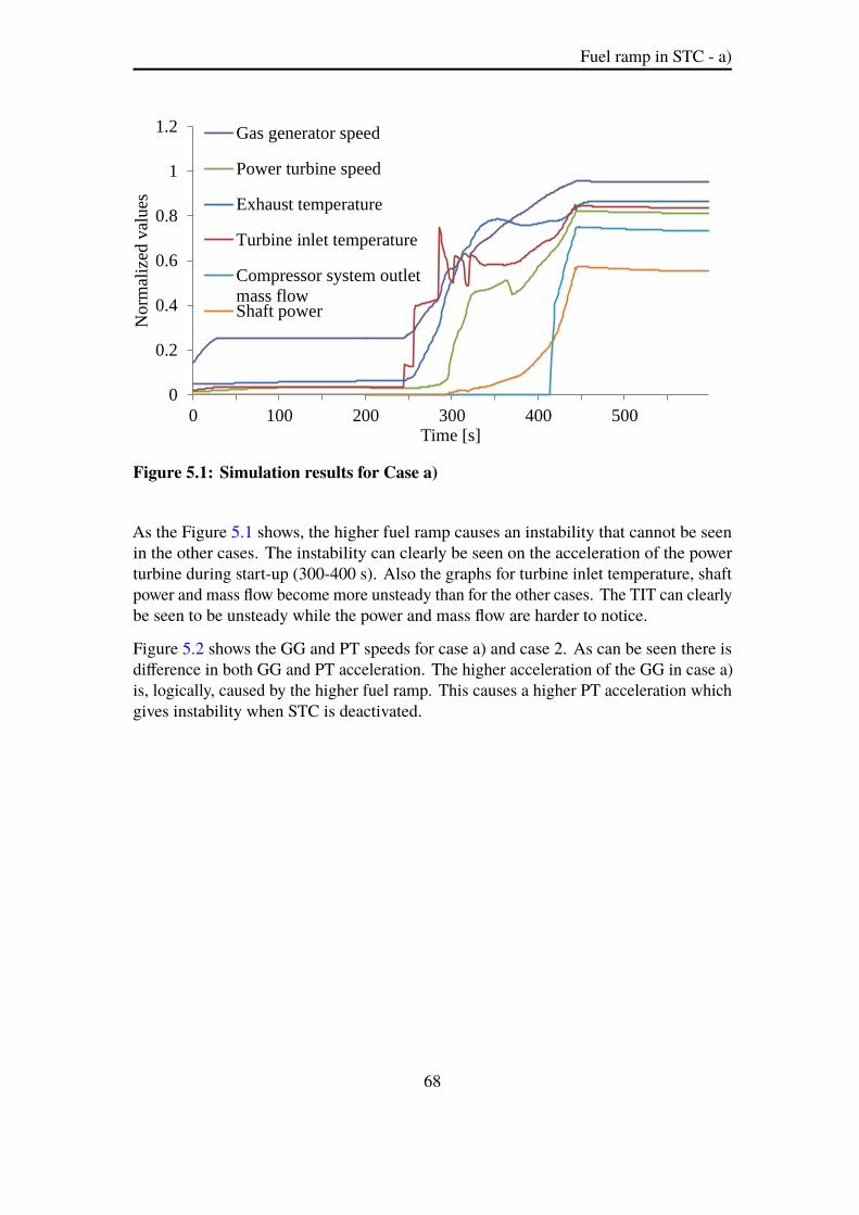
Fuel ramp in STC - a)

0

0.2

0.4

0.6

0.8

1

1.2

0 100 200 300 400 500

Norm

aliz

ed v

alues

Time [s]

Gas generator speed

Power turbine speed

Exhaust temperature

Turbine inlet temperature

Compressor system outlet

mass flowShaft power

Figure 5.1: Simulation results for Case a)

As the Figure 5.1 shows, the higher fuel ramp causes an instability that cannot be seenin the other cases. The instability can clearly be seen on the acceleration of the powerturbine during start-up (300-400 s). Also the graphs for turbine inlet temperature, shaftpower and mass flow become more unsteady than for the other cases. The TIT can clearlybe seen to be unsteady while the power and mass flow are harder to notice.

Figure 5.2 shows the GG and PT speeds for case a) and case 2. As can be seen there isdifference in both GG and PT acceleration. The higher acceleration of the GG in case a)is, logically, caused by the higher fuel ramp. This causes a higher PT acceleration whichgives instability when STC is deactivated.

68

5. BEHAVIOUR ANALYSIS

0

0,2

0,4

0,6

0,8

1

1,2

0 100 200 300 400 500

Norm

aliz

ed v

alues

Time [s]

Gas generator speed case a)

Gas generator speed case 2

Power turbine speed case a)

Power turbine speed case 2

Figure 5.2: Rotational speeds for case 2 and case a)

5.2 Rotational inertia - b)

Depending on what type of component the gas turbine drives, the rotational inertia varies.A higher inertia affect the acceleration of the component, and because the component isdirectly connected to the PT, it affects the PT acceleration as well. Figure 5.3 shows caseb), where this phenomena can be studied. It can be seen that the general behaviour issimilar to case 1, both during start-up and when ramping the mass flow set point.

69

Rotational inertia - b)

0

0.2

0.4

0.6

0.8

1

1.2

0 500 1000 1500 2000

Norm

aliz

ed v

alues

Time [s]

Gas generator speed

Power turbine speed

Exhaust temperature

Turbine inlet temperature

Compressor system outlet

mass flowShaft power

Figure 5.3: Simulation results for Case b)

Figure 5.4 shows case b), the same case as Figure 5.3 but with a zoomed view. One effectof the higher inertia is that the power turbine has a slower acceleration in the beginning,both during purge and just after ignition. Though it accelerates faster in the end of thestart-up due to its higher inertia and experiences a bit of an overshoot of the set value.This can also be seen in Figure 5.5, which shows the GG and PT speed for case b) andcase 1.

70

5. BEHAVIOUR ANALYSIS

0

0.2

0.4

0.6

0.8

1

1.2

0 100 200 300 400 500

Norm

aliz

ed v

alues

Time [s]

Gas generator speed

Power turbine speed

Exhaust temperature

Turbine inlet temperature

Compressor system outlet

mass flowShaft power

Figure 5.4: Simulation results for Case b), 600 s

0

0,2

0,4

0,6

0,8

1

1,2

0 100 200 300 400 500

Norm

aliz

ed v

alues

Time [s]

Gas generator speed case b)

Gas generator speed case 1

Power turbine speed case b)

Power turbine speed case 1

Figure 5.5: Rotational speeds for case 1 and case b)

71

Deactivation of PAC - c)

5.3 Deactivation of PAC - c)

As described in section 3.3 Dymola model of gas turbine control system, the PACcontrols the acceleration of the power turbine. Figure 5.6 shows a simulation with thePAC inactive.

0

0,2

0,4

0,6

0,8

1

1,2

0 100 200 300 400 500

Norm

aliz

ed v

alues

Time [s]

Gas generator speed

Power turbine speed

Exhaust temperature

Turbine inlet temperature

Compressor system outlet

mass flowShaft power

Figure 5.6: Simulation results for Case c)

In the figure that shows case c) it can be hard to compare the deviations between case 1(active PAC) and case c) (inactive PAC). For that reason Figure 5.7 shows a comparisonbetween the rotational speeds in the two cases. Even if the deviation is barely viewablethis indicates that the PAC does affect the start-up sequence. The reason to why theydiffer during such a small interval is that it is only during this time the PAC is active. Asthe figure shows the PAC lowers the acceleration slightly in this interval, as intended.The TIT is also seen to be more steady when the PAC is deactivated.

72

5. BEHAVIOUR ANALYSIS

0

0,2

0,4

0,6

0,8

1

1,2

0 100 200 300 400 500

Norm

aliz

ed v

alues

Time [s]

Gas generator speed case c)

Gas generator speed case 1

Power turbine speed case c)

Power turbine speed case 1

Figure 5.7: Rotational speeds for case 1 and case c)

5.4 Gas generator acceleration in NGGL - d)

As described in section 3.3 Dymola model of gas turbine control system, the NGGLcontrols the acceleration of the gas generator. In this case the limit of this acceleration isdecreased. This gives a slower acceleration for the gas generator during the time whenNGGL is active, at around 350 to 450 s. The simulation results can be seen in Figure 5.8.

73

0

0,2

0,4

0,6

0,8

1

1,2

0 100 200 300 400 500

Norm

aliz

ed v

alues

Time [s]

Gas generator speed

Power turbine speed

Exhaust temperature

Turbine inlet temperature

Compressor system outlet

mass flowShaft power

Figure 5.8: Simulation results for Case d)

Figure 5.9 shows a comparison between case d) and 1. This figure shows clearly how thegas generator acceleration differ between the cases. This causes the same difference forthe power turbine, as also can be seen in the figure.

0

0,2

0,4

0,6

0,8

1

1,2

0 100 200 300 400 500

Norm

aliz

ed v

alues

Time [s]

Gas generator speed case d)

Gas generator speed case 1

Power turbine speed case d)

Power turbine speed case 1

Figure 5.9: Simulation results for Case 1 and case d)

74

6. Discussion

The objective of this project was to design a model in Dymola that corresponds to realityand can be used in future work. The verification determined how large and what kind ofdeviations there were between reality and the model. In this section these deviations andrelationships are discussed.

6.1 Compressor model

The design of the compressor maps used as input caused inaccuracy for some parameters.Firstly, they have a limited range of speeds, why they had to be extended for speedsunder 50 %. To make the compressor model more accurate and complete it wouldbe advantageous to use maps with a wider range of speeds. Secondly, the dischargetemperature scale in the compressor maps causes deviations. Because it had to bemanually read and put into the model there is an uncertainty of the temperature outputand hence the polytropic efficiency. In this model it has been done as good as possible,according to the authors, but for future use a change of the compressor map design orformat would make it easier to add the data in the model and thereby make the outputfrom the compressor maps more accurate.

As mentioned in 3.2.3 Compressibility, the compressibility factor is included in themodel, though, it has to be manually added in two different locations which is notfavourable. The compressibility factor should be computed by Dymola instead to get theright density and inner energy.

6.2 Compressor train

The compressor train can be seen as a general model that can be used as a basic model torepresent different compressors, connected to a gas turbine. The aim was to agree asmuch as possible with the site El Encino, Mexico, where the general design originatesfrom. This does not mean that all parameters are tuned after this site. Many parameters

75

Verification

of for example the PID-controllers, has been chosen to fit this model specifically. Tomake the model more reliable more time has to be spent on various components. Asmentioned in 1.3 Limitations, focus has been to study the gas turbine behaviour, notspecific parameter values.

The control system of the gas turbine was carefully modified, to have the ability to usethe same control system in different applications. For example it is possible for the userto either choose PG or MD mode, and still use the same control system. Despite this,small changes had to be done in the gas turbine using this control system. This is notoptimal but the changes were necessary to be able to run the system in a MD mode.

6.3 Verification

6.3.1 Compressor system

When modelling the compressor system some limitations in Dymola were discoveredthat makes the thermodynamic calculations inaccurate. As mentioned in 4.1 Verificationof the compressor system, the enthalpy functions are not thermodynamically correct.Dymola calculates the enthalpy only with respect to temperature, which is a reasonableapproximation when calculating performance of a gas turbine. In this project however,the compressor inlet pressure is somewhere in the region of 50 bar instead of one barwhich then causes the model to behave inaccurate. The result of this was a low accuracyof the compressor power, which affects the shaft power of the gas turbine. To solve thisproblem major programming modifications needs to be done in Dymola, an objective toobig to include in this project. This is not a major problem though, because the purposeof the project was not to have exact values but to verify the behaviour of the system,which can be seen as accomplished. Due to the fact that the gas turbine only operates inregions far from critical regions it can be assumed that the enthalpy difference does notaffect the gas turbine behaviour.

The other verification parameters of the compressor system were in a reasonable range,according to the authors, when considering the limitations of the project. They differ lessthan 3 % which is acceptable as the temperature of the maps were difficult to implementin the model.

The verification of the compressor system was also about verifying the function of theanti-surge loop for the two cases. As illustrated in the previous chapter the surge marginis kept at 10 % by the anti-surge control system and the opening and closing of theanti-surge valve follows the prescribed times according to [21]. Since no data for thedriven unit could be found the behaviour of the compressor system was hard to tune in,in order to reflect reality and no further verification was performed.

76

6. DISCUSSION

6.3.2 Compressor train

The compressor train model is acting in a logical manner when analysing the figures inthe previous chapter. It serves its purpose as a model for the MD application with anSGT-750.

The activation of the different controllers can be seen in Figure 4.14. There are nounnecessary changes between the controllers which makes the model fast and stable.Of course there could be improvement in the different set points of the controllers toget an even smoother transition between them. As can be seen in Figure 4.13 the TITexperiences a quite unsteady behaviour, which could be dampened with tuning of thecontrollers. Though the TIT in reality never experiences these kinds of fluctuationsbecause of system inertia, but in the model the temperature is calculated and thereforebehaves in such an unstable manner. The controllers also fulfils their purpose of keepingdifferent critical parameters at, or above, their limits and the compressor train is thereforenever in any danger of entering surge or being accelerated too quickly during start-up.

Case 2 shows that the model can handle different inlet pressures in the compressorsystem, which is a case important for the validity of the model since the circumstancesof the pipeline, i.e. the inlet conditions of the compressor system changes over time.

6.3.3 Compressor maps

The compressor maps, Figure 4.16 and 4.17, show the operation line of case 1 and 3. Inboth cases the surge margin is decreased to the surge limit during start-up, this is doneto build up pressure in the driven compressor. It is unclear if that is the common wayduring start-up or if the valve is closed differently in order to keep a greater distance tothe surge limit. Since no measured data could be found for the surge margin, no furthertuning of the anti-surge valve was performed.

6.3.4 Eischleben and Port Said

As mentioned the machines compared were not the same and differs in their behaviourand performance so the shape of the curves were of more interest. The acceleration ofthe GG is similar to both sites while the PT speed differs more. A reason for this is ofcourse the fact that they are driving different compressors with different characteristicsand that the whole compressor train differs. Another reason could be the fact that theengine control differs between the machines. Different fuel ramps and different set pointsfor the different controllers contribute to the difference. The simulated PT speed startsfrom a higher speed than both Eischleben and Port Said which could be caused by theinaccuracy of the compressor and PT maps at speeds below 50 % of nominal speed.

77

Also the model is not able to start at too low speeds which is why there is a higher speedof the PT before ignition.

The start time of the simulation differs a bit from the start time of Port Said. Port Saidreaches its operating speed at approximately 800 seconds while the simulation reaches itat 500 seconds. This could be caused by different values of the controller parameters orthat they are different compressor trains as mentioned before. Though the start time ofEischleben is quite similar to the simulation which indicates that the start time can varyfrom machine to machine and that the model starts within a reasonable time space.

6.3.5 Behaviour analysis

The higher fuel ramp in case a) is seen to give a more unstable variation of the TIT,an uneven acceleration of the power turbine and a more unstable control of the systemwhich can be seen in Figure 5.1. This might be an indication that a lower fuel rampcould be advantageous during start-up for a compressor train with the SGT-750.

As the inertia was increased in case b) the model behaves in a similar way, but withslightly smaller transients which is what could be expected as the system gets slower inreacting to changes.

Case c), where the PAC is deactivated the behaviour of the TIT is more stable thanwhen the PAC is active. The unsteady behaviour is caused when the PAC decreasesthe temperature and the STC is activated once again and increases it, as can be seenin Figure 4.14. The simulations indicates that the PAC in this case has a small impacton the GG and PT speed acceleration. If so, the benefit of having the PAC can bequestioned. A deactivation gives a more stable and faster simulation but it is importantto note that the PAC may be necessary for other cases, depending on inertia and otherphysical limitations of the machine. For a machine with low inertia it would probably benecessary with an active PAC.

When changing the ramp of the NGGL in case d) the acceleration is of course slowerduring start-up and gives a slower starting of the compressor train. Except for that thereare small differences from case 1 and the time is the main parameter affected due to thischange.

78

7. Conclusions

• The objectives of the project was to create a model that corresponds to realityand can be connected to a gas turbine model. The verification shows that thecompressor system serves this purpose when connected to the gas turbine. Theauthors consider that the existing deviations is within approved area to regard it asa reliable compressor train model considering the limitations.

• As mentioned under 1.3 Limitations, the focus has been on analysing the behaviourof the gas turbine and only model the parts that affect the running of either the gasturbine or the compressor system. Thus, if the model is to be used for analysingspecific parameter values, the system components can be tuned in for that specificcase.

• The gas turbine control system is made as general as possible which makes itapplicable to different gas turbines and applications, both for PG and MD.

• The behaviour analysis shows that the lower fuel ramp affects the compressor trainin a positive manner for the simulated cases. It also shows that a deactivation ofthe PAC affects the compressor train in a positive manner for these specific cases.This indicates that the PAC might be redundant, but for other cases with differentinertia and physical behaviour it might be necessary to have a PAC. The ramp ofthe NGGL mainly affects the starting time and if a fast start is desired it should beas high as possible.

• With this model it is now possible to study how the gas turbine design can beoptimized for a MD application.

79

8. Future work

To further develop this project the following action points are suggested:

• Improve the medium handling in Dymola. To ensure correct enthalpy the functionsshould be modified to handle real gases where the enthalpy depends on bothtemperature and pressure.

• Add the compressibility factor in Dymola. The compressibility factor is in thisproject handled as a user input, where the user has to set the value in two differentlocations. This is not optimal and as future work the factor should be implementedinto the functions of the model and thereby be generated by Dymola.

• Simulate more scenarios. To make sure the model can handle a wide range ofpressures, mass flows and speeds more cases can be done. To be able to do this ina correct way more compressor maps should be implemented into the model. Thisaction needs digitalized compressor maps that easily can be used as input.

• Simulate larger systems. Considering the fact that many sites consist of severalcompressor trains it would be interesting to simulate this in Dymola. Connectingcompressor train models makes it possible to predict performance parameters for awhole compressor site.

81

9. References

[1] Kulturarv-Östergötland. Finspång. http://www.kulturarvostergotland.se/img/html_pobfin/html/finsp_indhi.html, 2003. Accessed: 2017-02-01.

[2] Kulturarv-Östergötland. Asea-stal. http://web.archive.org/web/20080207010024/http://www.808multimedia.com/winnt/kernel.htm,2003. Accessed: 2017-02-01.

[3] Rainer Kurz and Klaus Brun. Site performance test evaluation for gas turbine andelectric motor driven compressors, 2005.

[4] Meherwan P. Boyce. Gas Turbine Engineering Handbook. Gulf ProfessionalPublishing, third edition, 2006.

[5] R. L. Casper and R. E. Spector. The lm6000 gas turbine as a mechanical drivepower source. GE Marine & Industrial Engines, General Electric Company, 1992.

[6] P. E. Garrison T. E. Ekstrom. Gas turbines for mechanicaldrive applications. https://powergen.gepower.com/content/dam/gepower-pgdp/global/en_US/documents/technical/ger/ger-3701b-gas-turbines-mechanical-drive-applications.pdf.Accessed: 2017-04-06.

[7] Vivek Bhardwaj. Rotary compressors and types | work-ing principle | engineering explained. http://aermech.com/rotary-compressors-and-typesworking-principleengineering-explained,2015. Accessed: 2017-03-13.

[8] Peyman J. Positive displacement compressors: Re-ciprocating compressor. http://scopewe.com/positive-displacement-compressors-reciprocating-compressor/,2013. Accessed: 2017-03-13.

[9] H. Saravanamuttoo, G. Rogers, H. Cohen, and PV. Straznicky. Gas Turbine Theory.Pearson Education Ltd, sixth edition, 2009.

83

References

[10] Mecholic. Centrifugal compressor schematic dia-gram. http://www.mecholic.com/2016/07/centrifugal-compressor-parts-pressure-velocity-variation-curve.html, 2016. Accessed: 2017-03-13.

[11] Michael A. Boles Yunus A. Çengel. Thermodynamics - An Engineering Approach.McGraw-Hill, sixth edition, 2007.

[12] Frank Kreith. Mechanical Engineering Handbook. CRC Press LLC, first edition,1999.

[13] S.L. Dixon. Fluid Mechanics, Thermodynamics of Turbomachinery. Butterworth-Heinemann, fourth edition, 1998.

[14] A.M.Y Razak. Industrial gas turbines - Performance and operability. WoodheadPublishing Limited, first edition, 2007.

[15] E. M. Greitzer. Review - axial compressor stall phenomena. Journal of FluidsEngineering, 102:134–136, 6 1980.

[16] E. M. Graitzer. Surge and rotating stall in axial flow compressors. Journal ofEngineering for Power, pages 190–191, 1976.

[17] Christer von Wowern. PM about calculating polytropic efficiency with sT-method.Siemens Internal, 2012.

[18] Anna Sjunnesson. Interview. 4 2017.

[19] Bengt Sundén. Värmeöverföring. Studentlitteratur, Lund, 2006.

[20] John H. Lienhard IV and John H. Lienhard V. A Heat Transfer Textbook. PhlogistonPress, Massachusetts, third edition, 2005.

[21] Unknown. A surge philosophy. Siemens Internal, 2015.

[22] Karl Åström and Tore Hägglund. PID Controllers: Theory, Design, and Tuning.Instrument Society of America, second edition, 1995.

[23] PEDavid S.Moelling and Tetra Engineering Group Inc Peter S. Jackson, PE. Startuppurge credit benefits combined cycle operations. http://www.powermag.com/startup-purge-credit-benefits-combined-cycle-operations/, 2012.Accessed: 2017-05-23.

[24] Marie Kvilleng. SGT-750 Engine Control Specification. Siemens IndustrialTurbomachinery, f edition, 2016.

[25] Natural Gas Supply Association. Natural gas explained. https://www.eia.gov/energyexplained/?page=natural_gas_home, 2016. Accessed: 2017-03-14.

84

9. REFERENCES

[26] Editor E.W. McAllister. Pipeline, Rules of Thumb. Gulf Professional Publishing,fifth edition, 2002.

[27] Natural Gas Supply Association. The transportation of natural gas. http://naturalgas.org/naturalgas/transport/, 2013. Accessed: 2017-03-14.

[28] Siemens AG. Gas turbine sgt-750. http://www.energy.siemens.com/br/pool/hq/power-generation/gas-turbines/sgt-750/SGT-750_factsheet_en.pdf, 2016. Accessed: 2017-03-13.

[29] Siemens AG. Single shaft vertical split turbocompressors. http://www.energy.siemens.com/co/en/compression-expansion/product-lines/single-shaft-vertical-split/stc-sv.htm#content=Benefits, 2017.Accessed: 2017-04-07.

[30] Dassault Systems. Catia systems engineering - dymola. https://www.3ds.com/products-services/catia/products/dymola. Accessed: 2017-03-15.

[31] Flow Phase Inc. Vleflash. http://www.flowphase.com/Products/flash.html. Accessed: 2017-05-22.

[32] Bonnie J. McBride, Michael J. Zehe, and Sanford Gordon. Nasa glenn coefficientsfor calculating thermodynamic properties of individual species. https://www.grc.nasa.gov/WWW/CEAWeb/TP-2002-211556.pdf, 2002. Accessed: 2017-04-12.

[33] Pumps & Systems. Swing check valve. http://www.pumpsandsystems.com/images/stories/valves/val-maticfig1.jpg. Accessed: 2017-03-14.

[34] Alexandra Foley. How to model a shell and tube heat exchanger. https://www.comsol.com/blogs/how-model-shell-and-tube-heat-exchanger/,2013. Accessed: 2017-03-14.

[35] M.O. McLinden E.W. Lemmon and D.G. Friend. Thermophysical properties offluid systems in nist chemistry webbook, nist standard reference database number69, eds. p.j. linstrom and w.g. mallard, national institute of standards and technology,gaithersburg md, 20899, doi:10.18434/t4d303. Accessed: 2017-05-16.

85