7th aiaa/ceas aeroacoustics a01-30936 conferenceacoustique.ec-lyon.fr/publi/aiaa_2001_2226.pdf ·...

(c)2001 American Institute of Aeronautics & Astronautics or Published with Permission of Author(s) and/or Author(s)' Sponsoring Organization.

A01-309367th AIAA/CEAS AeroacousticsConference

28-30 May 2001 Maastricht, Netherlands

AIAA 2001-2226

Computation of the noise radiated by a subsonic cavityusing direct simulation and acoustic analogy *

Xavier Gloerfeltj" Christophe BaillyWd Daniel Juve§

Laboratoire de Mecanique des Fluides et d'AcoustiqueEcole Centrale de Lyon & UMR CNRS 5509

BP 163, 69131 Ecully cedex, France.

Abstract

The goal of this paper is to investigate the acoustic fieldgenerated by the flow over a cavity using two differentand complementary numerical methods. First, a DirectNumerical Simulation (DNS) of the 2-D compressibleNavier-Stokes equations is performed to obtain directlythe acoustic field. Second, this reference solution is com-pared to solutions provided by hybrid methods usingthe flowfield computed inside the cavity combined withan integral formulation to evaluate the far-field noise.Two integral methods are studied: the acoustic analogyof Ffowcs Williams and Hawkings (FW-H) and a waveextrapolation method based on FW-H equation. Bothshow a good agreement with DNS but the first one ismore expensive owing to an additional volume integral.The extrapolation method from a surface is more effi-cient and provide a complementary tool to extend CAAnear-field to very far field. These methods help the anal-ysis of wave patterns, by separating the direct wavesfrom the reflected ones.

1. Introduction

The computation of flow noise is a challengingproblem insofar as there are large disparities be-tween fluctuations in the flow and in the sound field.Energy radiated through the acoustic farfield is in-deed smaller than the one of the aerodynamic near-field by O(M4), and the involved length scales arevery different between the eddy scale and the acous-tic wavelength. The propagative nature of sounddiffers also greatly from the vortical behaviour of

* Copyright @ 2001 by the Authors. Published by theAmerican Institute of Aeronautics and Astronautics, Inc.,with permission.

tph. D. Candidate* Assistant Professor, Member AIAA§ Professor, Member AIAA

the flow. That's why approaches specific to aeroa-coustics have been developed. The first group ofapproaches separates the aerodynamic calculationand the noise propagation problem in order to ap-ply at each step the most appropriate method. Ba-sic difficulties in these so-called hybrid methods arethe modelling of the source terms from aerodynamicfluctuations and the ability of the wave operator toinclude complex acoustic-flow interactions. One ofthe first theories on aerodynamic noise generationwas given by the acoustic analogy of Light hill.1 Itwas extended by Ffowcs Williams and Hawkings2

(FW-H) to take the effects of solid boundaries intoaccount. This powerful analytical tool can be usedin connection with numerical methods to evaluatenoise radiation. Another relevant issue is the useof a surface integral formulation, like Kirchhoff's orporous FW-H methods, for prediction of the acous-tic field. These two approaches have similar an-alytical insights based on Green function formal-ism and suffer both from the limitation of the ob-server in a uniform flow. Linearized Euler Equa-tions (LEE) can provide a more complete propa-gation operator for acoustics in non-uniform me-dia. The coupling of these equations with a Navier-Stokes equations solver was demonstrated by Fre-und3 but offers only poor gain compared to directcalculation. Bailly et al.4 have introduced sourceterms in LEE with success for different free shearflows. The main difficulty is the modelling of thesource terms in more complex configurations. Wepropose here to study numerical issues of two in-tegral formulations: the Ffowcs Williams-Hawkingsanalogy and a wave extrapolation method (WEM)from a surface, sometimes called the porous FW-H integral method. However these two hybrid ap-proaches do not account for the aero dynamic-acous-tic coupling and they lack the modelling of the non-uniform flow effects.

1American Institute of Aeronautics and Astronautics


Turning to account the fact that both fluctu-ations are solutions of compressible Navier-Stokesequations, it is possible to obtain acoustic and aero-dynamic fields in the same calculation. However,owing to the great disparities between these twoquantities, in classical CFD (Computational FluidDynamics), acoustics is either not resolved accu-rately or not resolved because of the numerical sche-mes used and inadequate grid cell size or time step.Moreover, reflections due to the boundary conditionscan shade the physical acoustic wave field. That'swhy specific algorithms and appropriate boundaryconditions have been developed. We then talk aboutCAA (Computational Aero Acoustics). The CAAcodes essentially rest upon high order explicit sche-mes minimizing dispersion and dissipation of acous-tic waves. These choices are numerically expensivebut it is the price to make the aerodynamic flow andthe acoustic field coexist. CAA has already beenable to reproduce sound radiation from free flowslike a 3-D round jet5 with qualitatively and quanti-tatively good agreement with experimental data.

In this paper we focus our attention to imping-ing shear layer, which gives rise to intense coherentoscillations as well as associated noise radiation ina wide range of applications.6 The chosen test caseis a 2-D rectangular cavity, as well for its geometri-cal simplicity as for its relevance to many practicalconcerns. However, geometrical simplicity does notimply flow simplicity, and cavity flows provide anassortment of interesting theoretical questions andexperimental observations. The cavity flow, char-acterized by a severe acoustic environment withinand outside the cavity, arises from a feedback loop,locked in by the geometry and the flow characteris-tics. Despite numerous prior investigations, there re-main some central questions which must be adressedif an understanding of the self-sustained mechanismis to be achieved. We hope that aeroacoustic sim-ulations can provide a new tool to investigate howthe deformation of flow structures, their interactionswith the upstream edge, the dynamic of the sepa-rated shear layer, the internal recirculating flow orthe changes of flow regime with changing geometryand flow parameters are related to the intense radi-ated noise.

The aim of this paper is to study two integral hy-brid methods with direct computation as referenceand to evaluate their practical interest and comple-mentarity. In particular, for the case of cavity flowit is shown how these different tools can help us toanalyse the radiated acoustic field. In the first partof this paper, we shall present the direct computa-

tion of Navier-Stokes equations for a two-dimensio-nal rectangular cavity with aspect ratio of 2, pay-ing particular attention to the comparison betweenthese numerical results and Krishnamurty's exper-iments.7 In the second part, we shall describe thetwo integral methods based on FW-H equation andcompare the results to the DNS. We shall show howthese simulations can help the understanding of thenature of the acoustic radiations.

2. Direct computation of cavity noise

2.1 Introduction

Despite the amount of numerical studies pub-lished on cavity flows, few deal with radiated noise.Initial attemps have been made in supersonic cases.These first CFD computations of compressible cav-ity flows used the two dimensional unsteady RANS(Reynolds Averaged Navier-Stokes) equations with aturbulence model.8 The effectiveness of such mod-els for separated flows remains an open question.Slimon9 et al. have found that RANS simulationsshow a strong sensitivity to the choice of turbulencemodels. Tarn et al.10 showed that the results areaffected by high values taken by the turbulent vis-cosity. They even noticed better results for the es-timation of the time-averaged surface pressure fieldwith a zero-equation turbulence model. That's whyRona and Dieudonne11 preferred to study laminarflow motion. The absence of an eddy viscosity anda second-order algorithm give a moderate dispersionand dissipation. However, this choice, as well as theone of a relaxation length, is often made on an ad-hocbasis. To compute the broadband nature of cavitynoise at high Reynolds numbers, it is important totake account of the turbulent mixing. Zhang12 de-veloped an approach coupling the unsteady RANSequations and a k - u model including compressibil-ity corrections. But all these applications were per-formed with supersonic flows, simplifying the prob-lem.

The first computations of acoustic radiation froma cavity with a subsonic grazing flow have been car-ried out recently by Colonius13 et a!., and Shieh& Morris14 using 2-D Direct Numerical Simulation(DNS) at a Reynolds number based on cavity depthRep ~ 5000. These simulations show a transition toa new flow regime when the ratio L/60 of the cav-ity length over the momentum thickness becomeslarge. This mode is characterized by the sheddingof a single vortex which occupies all the cavity. Theperiodic ejection of this structure is associated with

American Institute of Aeronautics and Astronautics


an increase of the cavity drag. A similar transitionwas noted in the experiments of Gharib & Roshko15

in a water tunnel. The new regime was called wakemode because of the drag increase. However, thepresence of the wake mode has not been seen in ex-periments of compressible cavity flows at subsonicspeeds. The same numerical bifurcation has alsobeen noted by the authors.16 Does it result fromthe very low Reynolds numbers imposed by DNS orfrom the two-dimensional approach? To investigatehigher Reynolds numbers (Rep — 2 x 105), Shieh &Morris17 applied CAA tools to solve unsteady RANSwith a turbulence model: the one equation Spalart-Allmaras turbulence model and Detached Eddy Sim-ulation have been implemented. The transition to awake mode is still observed, indicating that it couldbe related to the 2-D behaviour rather than to theReynolds number. When the cavity length is largecompared to the thickness of the incoming boundarylayer, Najm & Ghoniem18 show in the same mannerthat the recirculation zone takes the form of a large-scale eddy that breaks away and migrates down-stream, overshadowing the role of the usual smaller-scale vortices. However, this too strong recirculatingflow is fed by the two-dimensional inverse cascade ofenergy. Vortex stretching, necessarily 3-D, shouldmodify significantly the turbulent mixing betweenthe clipped part of the shear layer and the corre-sponding counter-rotating vortex produced by theconservation of vorticity at the downstream edge.This turbulent mixing would prevent untimely tran-sition to wake mode. In our 2-D simulation, a shortaspect ratio and a relatively thick incoming bound-ary layer are chosen to ensure the shear layer modeof oscillations.

We try to reproduce numerically Krishnamurty'sexperiment7 with the same dimensions as in the ex-periment. The latter studied the acoustic radiationfrom two-dimensional rectangular cavities cut into aflat surface at low Reynolds numbers. The acousticfields were investigated by means of Schlieren obser-vations, interferometry, and hot-wire anemometer.The measurement used a cutout spanning the 4 by10 inch transonic wind tunnel and ending by a mov-ing plate to obtain cavities of various length L, thedepth D being the same for all of them, fixed at0.1 inch. We present here the simulation of the casewhere the length-to-depth ratio is 2 (L = 5.18 mmand D — 2.54 mm) where the boundary layer aheadof the cavity is laminar and the freestream Machnumber is 0.7. The Reynolds number based on cav-ity depth is Re& = 41000. The choice of a highsubsonic speed is interesting because the frequency

increases slightly with Mach number and the cavityis no more compact relatively to the acoustic wave-length. Moreover, the test case is more relevant forintegral methods because mean flow effects on soundpropagation become important.

2.2 Numerical methods

Governing equations

A Direct Numerical Simulation (no model) ofthe 2-D compressible Navier-Stokes equations is per-formed. The conservative form of these equations ina Cartesian coordinate system can be written as:

dU (9Ee <9Fe

dt dxi dx2

(9EV <9FV

8x2= 0

where:

U =

Ee =Fe =

Fv = (0,721, 722, Ml 721 + U2T22 + £2)*

The quantities p, p, HI are the density, pressure,and velocity components, while e and h are the to-tal energy and total enthalpy per mass unit. For aperfect gas,

h = e + p/pp = rpT

where T is the temperature, r the gas constant, and7 the ratio of specific heats. The viscous stress ten-sor nj is modelled as a Newtonian fluid and the heatflux component ^ models thermal conduction in theflow with Fourier's law:

+ _ k3 IJ dxk J

dT

where // is the dynamic molecular viscosity, a thePrandtl number, and cp the specific heat at constantpressure.

Algorithm

When the above equations are solved numeri-cally, it is imperative that, as the frequency is var-ied, neither the wave amplitude nor its propagation



speed be altered by the numerical scheme. That'swhy, following the work of Bogey,19 high order al-gorithms are implemented. The equations are ad-vanced in time using an explicit 4th order Runge-Kutta scheme.

The Dispersion-Relation-Preserving scheme de-veloped by Tarn and Webb20 is used to obtain spatialderivatives. A selective damping has also to be intro-duced in order to filter out non physical short wavesresulting from the use of finite differences and/ortreatment of boundary conditions.

Q 4

Figure 1: Computational grid for cavity L/D = 2(shown every other ten points). •: data sampling lo-cations for directivity evaluation. ( — — — ): locationof the progressive additional sponge zone.

Boundary treatment

This is the second key point of an aeroacous-tic simulation. We need nonreflecting conditions toavoid spurious reflections which can superpose tophysical waves. To this end, the radiation boundaryconditions of Tarn and Dong,21 using a polar asymp-totic solution of the linearized Euler equations in theacoustic far-field, is applied to the inflow and upperboundaries. At the outflow, we combine the out-flow boundary conditions of Tarn and Dong, wherethe asymptotic solution is modified to allow the exitof vortical and entropic disturbances, with a spongezone to dissipate vortical structures in the regionwhere the shear layer leaves the computational do-main. This sponge zone, represented in figure 1, usesgrid stretching and progressive additional dampingterms. Bogey et al.22 have shown its efficiency insituations where large amplitude non linear distur-bances must exit the domain without significant nu-merical reflections.

Along the solid walls, the nonslip condition ap-plies. The wall temperature Tw is calculated usingthe adiabatic condition. We keep centered differenc-

ing at the wall to ensure sufficient robustness usingghost points. This overspecification at the wall cangenerate spurious high-frequency waves which areeliminated by artificial damping.

Numerical specifications

The computational mesh, displayed in figure 1, isbuilt up from nonuniform Cartesian grid with 147 x161 points inside the cavity and 501 x 440 outside,highly clustered near the walls. The minimum stepsize corresponds to A?/^n = 0.8 in order to re-solve the viscous sublayer. The computational do-main extends over 8.5D vertically and Y1D hori-zontally to include a portion of the radiated field.The upstream and downstream boundaries are suf-ficiently far away from the cavity to avoid possibleself-forcing. The spacing between two points reachesa value Aymax = 2.9 x 10~5 m in the cavity andAymax = 5.6 x 10~5 m in the acoustic region.

The initial condition is a polynomial expressionof the laminar Blasius boundary layer profile for aflow at Mach 0.7. The initial boundary layer thick-ness at the cavity leading edge is SQ ~ 0.2D; itcorresponds to a ratio L/60 ~ 50, where L is thecavity length and SQ the momentum thickness. Thefreest ream air temperature T^ is 298.15 K and thestatic pressure p^ is taken as 1 atm.

Owing to the strong anisotropic computationalmesh, we have a very stiff discretized system. Forexplicit time marching schemes, an extremely smalltime step has to be used in order to satisfy thestability CFL criterion: A£ — 0.7 x A^^/COO =6.06 x 10~9 s. The mesh Reynolds number of theselective damping is chosen as RS = 4.5. This ar-tificial dissipation is applied a second time near thewalls and especially near the two edges.

The computation is 4 hours long on a Nee SX-5,with a CPU time of 0.4 //s per grid point and periteration.

2.3 Results and discussion

Far-field results

Figure 2 gives a monitored pressure history atx/D = —0.04 et y/D = 2D in the beginning of theacoustic region. The flow reaches a self-sustainedoscillatory state after a time of about 25D/t/oo butis still irregular until 65D/[/oo- During the first pe-riod, the natural cavity modes grow in amplitudeand saturate. Then transient is going on during thetime needed by the recirculating flow to get installedin the cavity.

The corresponding sound pressure level spectrum



5000

2500

r-~ oL

-2500

-50000 10 20 30 40 50 60 70 80

t*U/D

Figure 2: Pressure history versus time at x/D = —0.04and y/D = 2D.

160

140

-100

603St

Figure 3: Spectrum of pressure fluctuations at x/D—0.04 and y/D = 2D versus the Strouhal number St

is depicted in figure 3. It displays one principalpeak at St= 0.68, which corresponds to the periodicimpingement of coherent structures at frequency j3.Several secondary peaks are observable. The peaksat St= 1.39 and St= 2.14 are the first 2/3 and sec-ond 3/3 harmonics of principal frequency /3. Thelow-frequency component at /3/2 (St= 0.38) can beassociated with a low-frequency modulation by therecirculating zone, which alters periodically the av-erage trajectory of the incident vortex. Most ofthe noise energy is concentrated at the resonant fre-quency and its first harmonics. A Schlieren visu-alization, corresponding with vertical gradients ofdensity, shows the structure of the radiated fieldin figure 4(a). Two wave patterns are visible forthe positive gradients (dark), which interfer duringpropagation. Their strong upstream directivity ischaracteristic of high speed convection by the freestream. These radiations are in qualitatively goodagreement with the Schlieren picture of Krishna-murty (fig. 4(b)). The experimental Strouhal num-ber of oscillations is St= 0.71, corresponding to anerror of 5% on the frequency /3 found in our simu-lation. The Rossiter semi-empirical formula23 pro-vides St= 0.71 for this configuration with always twovortices in the shear layer.

Krishnamurty7 measured the intensity of acous-tic radiation through interferometry. He found thatthe acoustic field could be very intense with valuesgreater than 163 dB. These high intensity levels arealso found in the present simulation, with a magni-tude of sound pressure levels about 160 dB.

Q 4

Figure 4: Schlieren pictures corresponding to transver-sal derivative of the density: (a) present simulation, (b)Krishnamurty's experiment.7

Near-field results

The near-field is now investigated to try to iden-tify the noise generation mechanism, and in partic-ular to determine the origin of the two waves pat-terns noted previously. Figure 5 presents the vor-ticity field over one period of well-established self-sustained oscillations. In figure 5(a), the shear layeris seen to reattach at the trailing edge and two vor-tical structures can be identified in the shear layer.The first one is just shed from the leading edge sepa-ration. This rolled-up vortex travels downstream inthe next pictures, growing with convection. The sec-ond structure is located just upstream of the down-stream edge. As it impinges the edge (fig. 5(b)), theincident vortex is clipped at its centre. Part of thevortex spills over the cavity and is convected down-strean, increasing the thickness of the reattachedboundary layer. The other component is swept down-wards into the cavity creating recirculating regions(fig. 5(c)). In figure 5(d), the vortex generatedat the leading edge in the first picture arrives atthe trailing edge, sustaining the vortex impingementprocess.

The corresponding time matched pressure field isdepicted in figure 6. It is not easy to identify originsof noise generation because three different patternsare superposed. The first one is associated with thetwo coherent structures evolving in the shear layer.Low pressure regions in the shear layer identify vor-



(c)

(d)

Figure 5: Instantaneous vorticity contours at four timesduring one cycle. 16 contours between uiD/Uoo = —10.5and 1.36: (——— ) negative contours, (——— ) positivecontours. Zoom in and around the cavity.

3 4

Figure 6: Instantaneous pressure contours at four timesduring one cycle. 22 contours between —104 and 104

Pa: (——— ) positive contours, (---•---- ) negative contours.Zoom in and around the cavity.

tices, separated by high pressure regions. The twolow-pressure centers are clearly visible in fig. 6(d).The first one is associated with the vortex roll-upat the leading edge. The second one correspondsto the second vortex convected by the flow beforeit impinges the upsteam edge. The second pressurepattern represents the recirculating flow in the cav-ity. As seen in the vorticity snapshots, a principalrecirculation zone is located in the second half ofthe cavity, corresponding with the low pressure re-gion inside the cavity, identifiable in fig. 6(b) et 6(c).This large-scale region is not a single vortex but isactually made up of several smaller vortices, aris-ing from the clipping process, and its central regionis vorticity free. Endly, the third group of pressurewaves is the acoustic radiation generated by the flow.Figure 6 shows the birth of a positive pressure wavein the impingement process. The previously gener-ated wave, located at the leading edge in fig. 6(a),escapes from the cavity in fig. 6(d). In the latter

picture, the pressure wave seems to result from thesuperposition of two acoustic radiations. It is yetdifficult to identify the two sources in the presenceof interferences. This point will be discuss again inthe next part.

3. Validation of integral methods

3.1 Introduction

In the present simulation, the acoustic part ofthe mesh represents more than the half of the to-tal number of grid points, corresponding only to6 cavity depths. In order to ensure the six pointsper wavelength required by Tarn & Webb's sten-cil for the smallest acoustic wavelength present inthe computational domain (occuring here when adirect acoustic ray interfers with the reflected one),we have an acoustic cut-off Strouhal number Stc =fminL/Uov = L/(6A2/acousMoo) ~ 21. A reason-able calculation can then include only few wave-



lengths whereas realistic problems require observersat a distance of about two or three orders of magni-tude greater than the cavity length. For these dis-tances, it is certainly not discerning to perform adirect acoustic calculation.

The integral methods, instead, permit one to ob-tain the acoustic pressure at any points of the field,with a computational time independent of the ob-server distance. Typical calculations are carried outin two steps: an aerodynamic code based on CFD/CAA algorithms is used to evaluate the flow field,and then an integral formulation is applied to propa-gate the pressure disturbances in the farfield. Nume-rous integral methods are nowadays available. Theyrest upon two principal physical backgrounds: first,the acoustic analogies which split the computationaldomain in an aerodynamic region, where source ter-ms responsible for noise generation are built up, froman acoustic region governed by a linear wave equa-tion; second, the wave extrapolation methods whichallow the evaluation of the far-field once some quan-tities are known on a control surface. From a phys-ical point of view, it is important to notice that theextrapolation methods like Kirchhoff's formula arevalid for any phenomena governed by the linear waveequation like optics, acoustics or electromagnetismwhile the acoustic analogy is based on the conser-vation laws of mass, momentum, and energy and isthus dedicated to aeroacoustics.

Recent advances in integral methods were essen-tially developed for the reduction of helicopter rotornoise24 and have been recently applied for the pre-diction of jet noise.25'26 Zhang, Rona, and Lilley27

have used Curie's spatial formulation to obtain far-field spectra of cavity noise but no validation wereproposed.

3.2 Acoustic analogyThe acoustic analogy was proposed by Lighthill1

and was extended by Curie28 and Ffowcs Williamsand Hawkings2 to include the effects of solid sur-faces in arbitrary motion. The FW-H equation isan exact rearrangement of the continuity equationand Navier-Stokes equations into the form of an in-homogeneous wave equation with two surface sourceterms and a volume source term. The use of general-ized functions to describe flow quantities permits oneto embed the exterior flow problem in unboundedspace. An integral solution can thus be obtained byconvoluting the wave equation with the free-spaceGreen function.

A serious restriction is that the observation re-gion is assumed at rest. It is difficult to extend

the propagation operator to include more complexflows. Only the case of a uniform flow is satis-factorily treated. Ffowcs Williams and Hawkingsproposed the use of a Lagrangian coordinate trans-form assuming the surface is moving in a fluid atrest. Goldstein29 preferred to take the convectioneffects in the wave equation. In the same man-ner, in the case of a motion with constant velocityUQO = (t/i,0), the application of the Galilean trans-formation from the observer position (x,£) to (77,?),

r]i = Xi + Uit, t — t

leads to the convected FW-H equation30:

JL (3(77,+ (i)where the modified source terms including convec-tion can be written as:

fij = p(ui - Ui)(uj - Uj) + [p - clop] 8ij - nj (2)dfFi = [p00UiUj+p8ii-nj]

Q = \-P~U*}

(3)

(4)

H is the Heaviside function and the function / = 0defines the surface E outside of which the densityfield is calculated. / is scaled so that df/drjj — %,the j-component of the unit normal vector pointingtoward the interior of E. For a rigid body, we havesimplified the surface source terms using the non-penetrating condition un — u.n = 0.

For bidimensional geometries, it is more conve-nient to resolve this equation in the spectral do-main.30 The frequency domain formulation avoidsthe evaluation of the retarded time in three-dimen-sional problem, which can be a critical point. Thegain over the time-domain applications is enhancedin 2-D because of the weaker properties of the Heav-iside function which replaces the Dirac function in 2-D Green functions. Whereas the Dirac leads to a re-tarded time expression removing the temporal inte-gration, the Heaviside function can only change theupper limit of the integration to a finite value, thelower limit remaining infinite. The spectral formu-lation removes this time constraint by solving FW-H equation harmonically. With application of theFourier transform

-fJ — c(x,t)e~iujt dt (5)



equation (1) becomes

(6)

where M« = Ui/Coo. A Green function for this in-homogeneous convected wave equation is obtainedfrom a Prandtl-Glauert transformation of the 2-Dfree-space Green's fonction in the frequency domain:

i(Mk(rll-yl)/!32

= — e

where r2 - (771 - yi)2 + /32(r?2 - 2/2)2, #Q2) is the

Hankel function of the second kind and order zero,and /3 = v 1 — M2 is the Prandtl-Glauert factor,M< 1. The integral solution of equation (6) is thengiven by:

r ~Jf=or .• I iu

Jf=0

J J f>0

^G(rj\y)

y)

(7)

In 2-D, the volume integral is restricted to thesurface So (/ > 0) including the aerodynamic sourcesTij and the surface integrals are calculated on thesolid lines which represent rigid boundaries. We ap-plied the spatial derivatives on the Green function toavoid the evaluation of derivatives of aerodynamicquantities. It is formally equivalent to the trans-formation in temporal derivatives as performed byDiFrancescantonio31 or Farassat and Myers.32

3.3 Wave extrapolation method

This kind of methods permits one to solve lin-ear wave propagation problem once some flow quan-tities are given on a closed fictitious surface sur-rounding all the sources. The most famous one isthe Kirchhoff 's method which makes a parallel withelectromagnetism by using KirchhofFs formula. Themain advantage with respect to acoustic analogy ap-proaches is that only surface integrals have to beevaluated because all non linear quadrupolar sourcesare enclosed in the control surface. The problem is

thus reduced by one dimension, which is particularlyinteresting in a numerical point of view. However,this approach suffers from the restriction that Kirch-hoff's surface must strictly be in the linear acousticregion. Brentner and Farassat33 and Singer34 et al.show some misleading results when Kirchhoff's for-mulation is applied respectively to a hovering rotorblade and to the flow past a circular cylinder byusing a control surface too close to the sources orcrossing a shear layer.

A very clear analysis given by Brentner24 showsthat a wave extrapolation method based on the FW-H equation is relatively unaffected by the placementof the integration surface unlike Kirchhoff's formula-tion. We note FW-H WEM the Wave ExtrapolationMethod based on the FW-H formulation (7) by ne-glecting the volume integration (quadrupole sourceterm Ty). This FW-H WEM can combine the flex-ibility of the Kirchhoff's method and the physicalinsights of the FW-H equation.

FW-H and Kirchhoff formulations solve the samephysical problem, the differences between the twowritings being due to some choices made in the deriva-tion process. In particular, the volume term of theKirchhoff's formula include strictly all nonlinear as-pects whereas a part of these aspects is moved inthe dipole and monopole surface integrals in FW-Hformulation. As a result, the two formulations workwell when the control surface is in the far-field regionbut if it lies in a not-fully linear region, the Kirch-hoff's results are erroneous and the FW-H WEMis more efficient. This method is sometimes calledporous FW-H because it coincides with the applica-tion of FW-H analogy on a fictitious porous surface.The analytical developments are the same that thoseof FW-H analogy but the non-penetration conditionun — 0 is no more required, and, in order to obtaincorrect results, one has to allow a fluid flow acrossS.

For a two-dimensional problem with uniform sub-sonic motion, FW-H WEM is given by equation (7)without the volume integral:

- I iJf=0

with the two source terms:

Q^^-p^jL

) W )G( i j | y )dE (8)

•H-rii]^- (9)3 n Ox, v '

(10)



3.4 Numerical implementation

I D • — - — • — - — • — • — .•—- — -.--0.5 D- . . . . . . . . . . . . . . ; . . .0.2 D------------.---

-5 D -2 D

V • •^1

S2si

O D 2D

Figure 7: Schematic of the different line and surfacesources for evaluation of integral formulations.

The fact that the FW-H equation can be the ba-sis for either an acoustic analogy or a wave extrap-olation method permits us to develop a single code.The choice of the method is made by neglectingthe volume integral or imposing the non-penetrationcondition.

From an algorithmic point of view, there is al-most no difference between the two approaches con-sidered here. The first step is the recording of theaerodynamic quantities during one period of the DNScomputation, using the pseudoperiodic behaviour ofthe oscillations in the cavity. The acoustic time stepis 40 times the DNS time step corresponding to 131points per wavelength. The variables (ui,u<2,p,p)are recorded on three fictitious lines of the meshgridfor wave extrapolation method, and on the walls ofthe cavity and the surface around it for the acousticanalogy application as reported in figure 7.

Then the source terms are calculated and trans-formed in the frequency-domain using the Fouriertransform defined by (5) for the positive frequen-cies. The contribution of the negative counterpartis equal and can be taken in account by doublingthe final result. The integrals are then evaluatedfor each point of an acoustic meshgrid. This regu-lar cartesian grid of 176 x 184 points covers a areaof (-5£>;5£>) x (-1D;8£>), corresponding with themain part of acoustic domain of DNS. Endly, an in-verse Fourier transform is used to recover the acous-tic signal in time-domain.

3.5 Results of porous FW-H

The extrapolation is performed from three linesspanning the longitudinal direction, of 501 points.The first line LI is chosen in the acoustic region aty = ID where a Kirchhoff's method would also havebeen applied. The second line L2 is in the near-fied region at y = 0.5.D, and the third line Z/3 isstill closer to the shear at y = O.2.D. The results ofintegration over LI, L2, and L3 with source termsdefined by (9), and (10), and with M^ = 0.7 in

Figure 8: Pressure field calculated at the same time by(a) FW-H WEM from LI, (b) FW-H WEM from L2, (c)FW-H WEM from L3, (d) DNS.

the observer domain are compared in figure 8. Thethree pressure fields obtained are consistent with theDNS. The contour plots are sharper when the sur-face is farther from sources. This is confirmed by thepressure profile of figure 9, and by the overall soundpressure directivity of figure 10. The three profilespredicted by the FW-H WEM are in good agreementwith the DNS result. The small differences could beattributed to the fact that not all of the quadrupolarsources are taken into account when the integrationsurface is too close to the walls.

3.6 Results of FW-H analogy

When we apply FW-H analogy, the surface inte-grals are evaluated on the physical rigid walls of thecavity (solid lines of figure 7). The good results ofporous FW-H method on L3 placed at y - 0.2£> in-dicates that the volume sources above this line wouldbe negligible. In the present evaluation, the chosenvolumes are depicted in figure 7: 52 is the surfaceinside the cavity, and 5i the surface above it. S\ isID high, and extends from — 2D to 5L> in stream-wise direction. However, the evaluation of volumeintegrals of Tij are sensible to truncature effets, es-pecially in the streamwise direction where the sourceterms decrease slowly. It is due to the presence of ad-vected vortices, ejected from the cavity during the


(c)2001 American Institute of Aeronautics & Astronautics or Published with Permission of Author(s) and/or Author(s)1 Sponsoring Organization.

4000

-4000

r/D

Figure 9: Pressure profile along the line x-2D=-y ob-tained by: ( - - - - ) FW-H WEM from LI, ( • • • • • • )FW-H WEM from L2, (- - - ) FW-H WEM fromL3,

60 80 100 1206 (deg)

160 180

Figure 10: Overall sound pressure level as function of 9measured from streamwise axis, evaluated on the sensorsreported in figure 1. Same legend as fig. 9

clipping process, in the reattached boundary layeron the downstream wall.

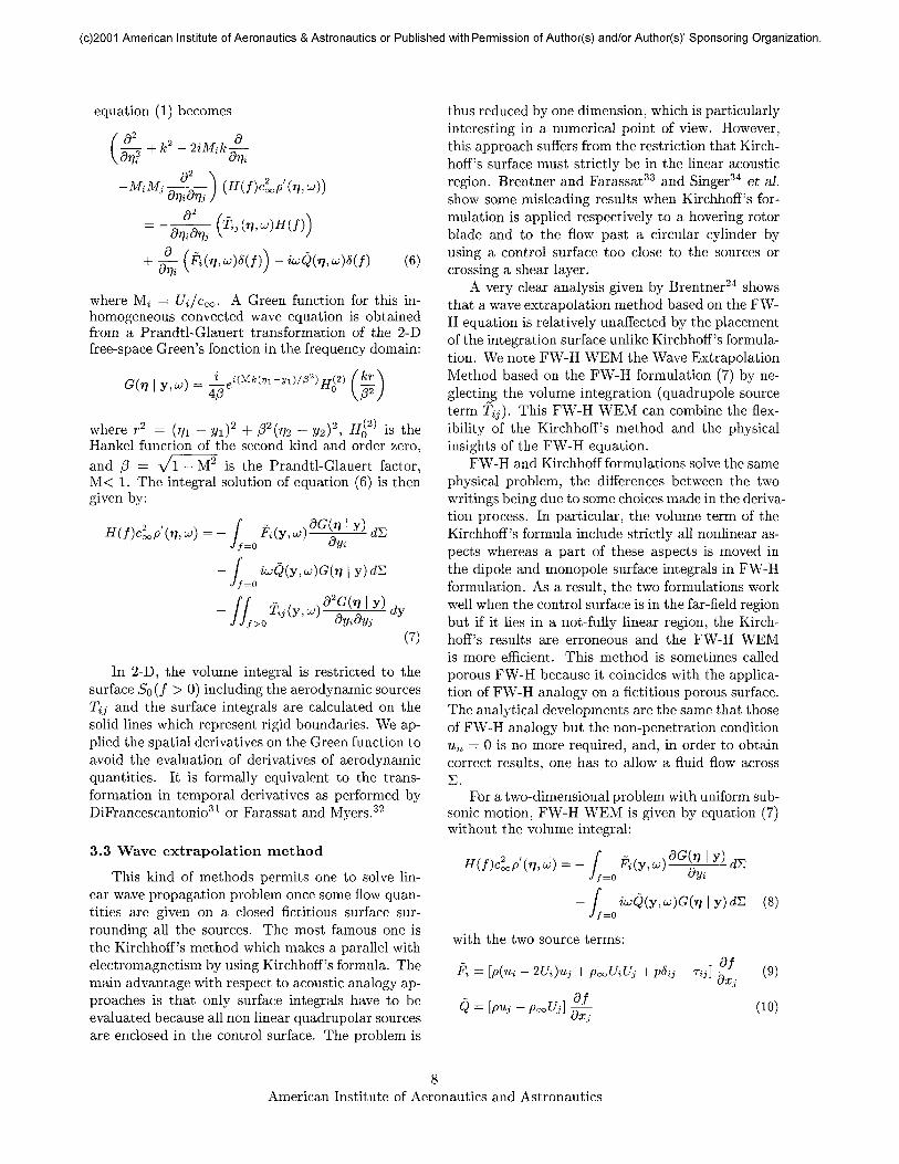
To obtain the volume integral part of the radi-ated sound field, we add the contributions of Si and52 (figure 11 (a)). The surface integration is per-formed on cavity walls with source terms defined by(3) and (4), with MOO =0.7. The result is depictedin figure ll(b). Following reflection theorem of Pow-ell,35 we can argue that volume integrals representthe direct radiated field, and surface integrals showessentially the reflected part of the field due to cavitywalls. By summing the volume and surface contri-butions (fig. 12(a)), we reconstruct the total soundfield in reasonably good agreement with the DNSreference solution of figure 12(b). Figure 13 showsthat the pressure profile along the line x + y = IDis consistent with direct calculation.

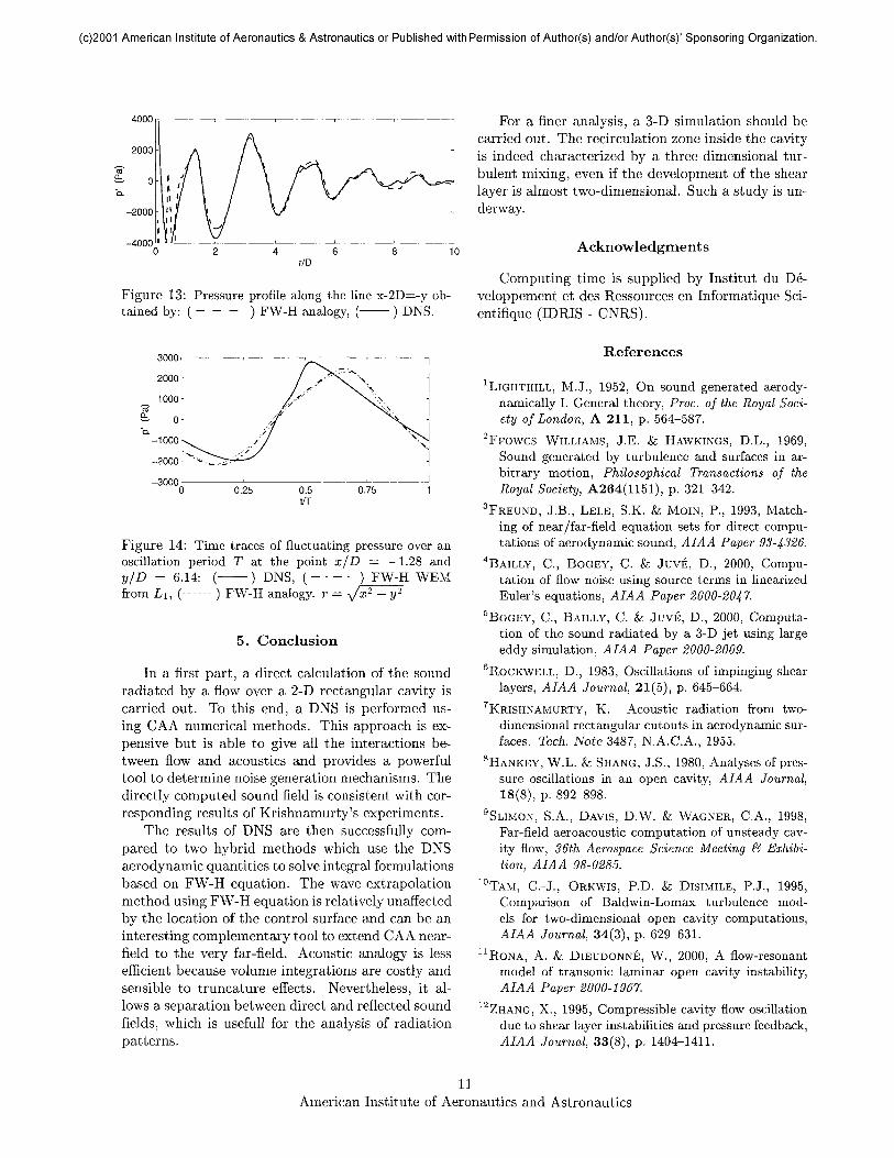
Figure 14 presents the temporal evolutions of thepressure over one period using the three methods.DNS results show a very stiff slope for the temporalevolution, which indicates a non-linear propagation.The two integral formulations time traces have a si-nusoidal shape. The non-linear effects are indeednot taken into account in integral methods since the

Figure 11: Pressure field obtained corresponding to: (a)volume integral part of FW-H analogy, and (b) surfaceintegral part of FW-H analogy.

volume integral is neglected in FW-H WEM and thevolume integral does not include all the non-linearregion in FW-H analogy.

Figure 12: Pressure field calculated at the same timeby (a) FW-H analogy (surface + volume integrals), (b)DNS reference solution.

The FW-H analogy provides more informationsthan the WEM but is more expensive in CPU timebecause of the evaluation of volume integral (surfaceintegral in 2-D) whereas wave extrapolation methodsneed only surface integral (line integral in 2-D). Forexample, the computation time needed by the FW-H WEM is around 13 minutes, whereas the FW-Hanalogy requires 17 hours, on a Dec a computer. Forthe purpose of comparison, the DNS would take 320hours on this machine.

FW-H analogy allows a better understanding ofthe structure of the radiated field than WEM. Inparticular, the direct and reflected sound field canbe separated. These two fields at the same frequencygive an interference figure where the two waves pat-terns are still distinguishable in our case because thecavity is not compact at the oscillation frequency(L/A = 0.47).



4000

2000

^ oL

-2000

-4000

Q.

10r/D

Figure 13:tained by: (

Pressure profile along the line x-2D=-y ob-- - - ) FW-H analogy, (——— ) DNS.

For a finer analysis, a 3-D simulation should becarried out. The recirculation zone inside the cavityis indeed characterized by a three-dimensional tur-bulent mixing, even if the development of the shearlayer is almost two-dimensional. Such a study is un-derway.

Acknowledgments

Computing time is supplied by Institut du De-veloppement et des Ressources en Informatique Sci-entifique (IDRIS - CNRS).

3000

2000

1000

I 0

-1000

-2000

-30000.25 0.5

\fT0.75

Figure 14: Time traces of fluctuating pressure over anoscillation period T at the point x/D = —1.28 andy/D = 6.14: (———) DNS, ( - - - - )_FW-H WEMfrom LI, (•- FW-H analogy, r —

5. Conclusion

In a first part, a direct calculation of the soundradiated by a flow over a 2-D rectangular cavity iscarried out. To this end, a DNS is performed us-ing CAA numerical methods. This approach is ex-pensive but is able to give all the interactions be-tween flow and acoustics and provides a powerfultool to determine noise generation mechanisms. Thedirectly computed sound field is consistent with cor-responding results of Krishnamurty's experiments.

The results of DNS are then successfully com-pared to two hybrid methods which use the DNSaerodynamic quantities to solve integral formulationsbased on FW-H equation. The wave extrapolationmethod using FW-H equation is relatively unaffectedby the location of the control surface and can be aninteresting complementary tool to extend CAA near-field to the very far-field. Acoustic analogy is lessefficient because volume integrations are costly andsensible to truncature effects. Nevertheless, it al-lows a separation between direct and reflected soundfields, which is usefull for the analysis of radiationpatterns.

References

^IGHTHILL, M.J., 1952, On sound generated aerody-namically I. General theory, Proc. of the Royal Soci-ety of London, A 211, p. 564-587.

2Frowcs WILLIAMS, J.E. & HAWKINGS, D.L., 1969,Sound generated by turbulence and surfaces in ar-bitrary motion, Philosophical Transactions of theRoyal Society, A264(1151), p. 321-342.

3FREUND, J.B., LELE, S.K. & MOIN, P., 1993, Match-ing of near/far-field equation sets for direct compu-tations of aerodynamic sound, AIAA Paper 93-4326.

4BAiLLY, C., BOGEY, C. & JUVE, D., 2000, Compu-tation of flow noise using source terms in linearizedEuler's equations, AIAA Paper 2000-2047.

5BoGEY, C., BAILLY, C. & JUVE, D., 2000, Computa-tion of the sound radiated by a 3-D jet using largeeddy simulation, AIAA Paper 2000-2009.

6ROCKWELL, D., 1983, Oscillations of impinging shearlayers, AIAA Journal, 21(5), p. 645-664.

7KRISHNAMURTY, K. Acoustic radiation from two-dimensional rectangular cutouts in aerodynamic sur-faces. Tech. Note 3487, N.A.C.A., 1955.

8HANKEY, W.L. & SHANG, J.S., 1980, Analyses of pres-sure oscillations in an open cavity, AIAA Journal,18(8), p. 892-898.

9SLiMON, S.A., DAVIS, D.W. & WAGNER, C.A., 1998,Far-field aeroacoustic computation of unsteady cav-ity flow, 36th Aerospace Science Meeting & Exhibi-tion, AIAA 98-0285.

10TAM, C.-J., ORKWIS, P.D. & DISIMILE, P.J., 1995,Comparison of Baldwin-Lomax turbulence mod-els for two-dimensional open cavity computations,AIAA Journal, 34(3), p. 629-631.

11RONA, A. & DIEUDONNE, W., 2000, A flow-resonantmodel of transonic laminar open cavity instability,AIAA Paper 2000-1967.

12ZHANG, X., 1995, Compressible cavity flow oscillationdue to shear layer instabilities and pressure feedback,AIAA Journal, 33(8), p. 1404-1411.



13CoLONius, T., BASU, A.J. & ROWLEY, C.W., 1999,Numerical investigation of the flow past a cavity,AIAA Paper 99-1912.

14SniEH, C.M. & MORRIS, P.J., 1999, Parallel numericalsimulation of subsonic cavity noise, AIAA Paper 99-1891.

15GHARIB, M. & ROSHKO, A., 1987, The effect of flowoscillations on cavity drag, J. Fluid Mech., 177, p.501-530.

16GLOERFELT, X., BAILLY, C. & JUVE, D., 2000, Calculdirect du rayonnement acoustique d'un ecoulementaffleurant une cavite, C. R. Acad. Sci., t. 328, Serielib.

17SHIEH, C.M. & MORRIS, P.J., 2000, Parallel computa-tional aeroacoustic simulation of turbulent subsoniccavity flow, AIAA Paper 2000-1914.

18NAJM, H.N. & GHONIEM, A.F., 1991, Numerical sim-ulation of the convective instability in a dump com-bustor, AIAA Journal, 29(6), p. 911-919.

19BOGEY, C. Calcul direct du bruit aerodynamique etvalidation de modeles acoustiques hybrides. PhD the-sis, Ecole Centrale de Lyon, 2000. No 2000-11.

20TAM, C.K.W. & WEBB, J.C., 1993, Dispersion-relation-preserving finite difference schemes for com-putational acoustics, J. Comput. Phys., 107, p. 262-281.

21TAM, C.K.W. & DONG, Z., 1996, Radiation and out-flow boundary conditions for direct computation ofacoustic and flow disturbances in a nonuniform meanflow, J. Comput. Acous., 4(2), p. 175-201.

22BOGEY, C., BAILLY, C. & JUVE, D., 2000, Numericalsimulation of sound generated by vortex pairing in amixing layer, AIAA Journal, 38(12), p. 2210-2218.

23RossiTER, J.E. Wind-tunnel experiments on the flowover rectangular cavities at subsonic and transonicspeeds. Technical Report 3438, Aeronautical Re-search Council Reports and Memoranda, 1964.

24BRENTNER, K.S., 2000, Modeling aero dynamicallygenerated sound: Recent advances in rotor noise pre-diction, AIAA Paper 2000-0345.

25CoLONius, T. & FREUND, J.B., 2000, Applicationof Lighthill equation to a Mach 1.92 turbulent jet,AIAA Journal, 38(2), p. 368-370.

26BoGEY, C., BAILLY, C. & JUVE, D., 2001, Noise com-putation using LighthilPs equation with inclusionof mean flow - acoustics interactions, AIAA Paper2001-2255.

2 7ZHANG, X., RONA, A. & LILLEY, G.M., 1995, Far-fieldnoise radiation from an unsteady supersonic cavity,AIAA Paper 95-040.

28CuRLE, N., 1955, The influence of solid boundariesupon aerodynamic sound, Proc. of the Royal Societyof London, A 231, p. 505-514.

29GOLDSTEIN, M.E., 1976, Aeroacoustics, McGraw-Hill,New York.

30LocKARD, D.P., 2000, An efficient, two-dimensionalimplementation of the Ffowcs Williams and Hawk-ings equation, J. Sound Vib., 229(4), p. 897-911.

31Di FRANCESCANTONIO, P., 1997, A new boundary in-tegral formulation for the prediction of sound radia-tion, J. Sound Vib., 202(4), p. 491-509.

32FARASSAT, F. & MYERS, M.K., 1988, Extension ofKirchhoff's formula to radiation from moving sur-faces, J. Sound Vib., 123(3), p. 451-460.

33BRENTNER, K.S. & FARASSAT, F., 1998, An analyticalcomparison of the acoustic analogy and Kirchhoff for-mulation for moving surfaces, AIAA Journal, 36(8),p. 1379-1386.

34SiNGER, B.A., BRENTNER, K.S., LOCKARD, D.P. &LILLEY, G.M., 2000, Simulation of acoustic scatter-ing from a trailing edge, J. Sound Vib., 230(3), p.541-560.

35POWELL, A., 1960, Aerodynamic noise and the planeboundary, J. Acoust. Soc. Am., 32(8), p. 982-990.


7th aiaa/ceas aeroacoustics a01-30936 conferenceacoustique.ec-lyon.fr/publi/aiaa_2001_2226.pdf ·...

Documents