774 kcmil accr sag and amp

7/27/2019 774 Kcmil ACCR Sag and Amp

http://slidepdf.com/reader/full/774-kcmil-accr-sag-and-amp 1/18

To: Dr. Colin McCullough

Specialty Materials DivisionComposite Conductor Program3M Company3130 Lexington Ave SoEagan, MN 55121USA

KINECTRICS NORTH AMERICA INC. TEST REPORTFOR 3M COMPANY TO DETERMINE THE SAG – TEMPERATURE – TENSION

PERFORMANCE OF 774 KCMIL 3MTM COMPOSITE CONDUCTOR

Kinectrics North America Inc. Report No.: K-422132-RC-0001-R00September 26, 2005

C.J. PonTransmission and Distribution Technologies Business

INTRODUCTION

A Sag – Temperature – Tension Test was performed for 3M Company on their 3MTM CompositeConductor, which is also known as Aluminium Conductor Composite Reinforced (ACCR)Conductor. This test is part of a larger series of tests to demonstrate the viability of ACCRconductors for use on overhead electric power transmission lines. The tests were performed byKinectrics North America Inc. personnel at 800 Kipling Avenue, Toronto, Ontario, M8Z 6C4,Canada. 3M owns all data and copyright to this information.

A sag-tension-temperature study on 774 kcmil ACCR showed a knee-point transition in the

region of 60°C. The “compressive stress parameter” or “built-in tensile stress parameter” shouldbe set at -1.45 ksi (-10 MPa) for the line design software programs. The line design softwareprograms such as Alcoa Sag10TM software and STESS predict the sag-tension-temperaturebehaviour very well.



TEST OBJECTIVE

The objective of the Sag – Temperature – Tension Test was to determine the sag and tension ofthe 774 kcmil ACCR conductor when subjected to increasing temperatures. The compositecore of 3M’s ACCR conductors has a lower coefficient of thermal expansion and higherconductivity than the steel core in conventional ACSR conductors. The Sag – Temperature –

Tension Test tests would provide information on whether these differences affect the thermaland physical response of the ACCR conductors.

Additional information on the current-temperature relationship for the conductor was obtained byselecting several arbitrary current levels and measuring the resulting temperature. Thesemeasurements were performed at known conditions so the results could be compared toampacity calculations based on IEEE Std 738. The known conditions would be no wind, no sun,ambient temperature and altitude. The conductor was essentially in “new” condition so theemissivity and absorptivity could be estimated to produce a best fit to the calculations.

TEST CONDUCTOR

The conductor tested was designated ACCR-774-T53, 46/37 manufactured by 3M Company.The construction of this conductor has 46 heat-resistant aluminum-zirconium alloy wires in 2layers surrounding 37 core wires in 3 layers. The outside diameter of the conductor is 1.254inches (28.1mm). The rated tensile strength (RTS) of the conductor is 71,010 lbf (32,210 kgf).This particular conductor construction has a high core fraction (33% core by area), and is anexample of a construction intended for use in long span crossings.The data sheet on the 774 kcmil ACCR conductor used in the sag – temperature – tension testis contained in Appendix A.

Approximately thirty-nine (39) meters of the conductor was prepared. The conductor wasterminated as shown in Figure 1. Each end of the conductor was passed through aluminum

housings. The conductor strands were splayed apart within a cone-shaped cavity inside thealuminum housing. High-temperature epoxy resin was poured into the cavity to “lock” allstrands of the conductor together. The strands were reformed outboard of the aluminumhousing and a compression terminal was compressed on the end of the conductor to allowcurrent to be passed through the sample.

Figure 1 Epoxy Dead-end

2 K-422132-RC-0001-R00



TEST SET-UP

Test Apparatus

The Sag – Temperature – Tension Test was carried out at Kinectrics’ Conductor Dynamics

Laboratory. The laboratory is temperature controlled to 22ºC ±2ºC with minimal air movement. A schematic of the setup is shown in Figure 2. The maximum span length (i.e. tension eye totension eye) was 39.9 m. The actual conductor length was shorter than this to accommodateend hardware such as the tensioning dead-ends, insulators, load cells and other links. Thesample was tensioned horizontally about 2.44m (8 feet) above the ground.

A-A Overall span length (68.8 m) G North Load CellB-B Span length between North and South Sag Measurement H North Insulator (4 skirt)C-C Sag at mid-span J North epoxy dead-end assemblyD-D Sag at North end just inboard of hardware K South Load CellE-E Sag at South end just inboard of hardware L South Insulator (6 skirt)F Strain Plate M South epoxy dead-end assembly

Figure 2 Schematic of Test Setup

A current transformer provided the circulating current to heat the cable. One end of theconductor was connected to a tap of the current transformer. The opposite end of the conductorwas connected to two large ACSR conductors, (return conductor) to complete the circuit back tothe current transformer. The return conductors were untensioned and were positioned oninsulating pads on the floor.

Instrumentation

Conductor Tension

A strain gauge load cell measured the tension in each conductor during the test. The load cellwas installed between the insulator and the dead-end structure so that it would be electrically

isolated from the conductor. The signal from the load cells were amplified by optically isolatedsignal conditioners to provide a 0 to 5 volt signal for the data acquisition system.

Conductor Temperature

The temperature of the conductor was measured at two(2) locations using thermocouples. Onelocation was at the centre of the span the other location was at halfway between the centre andone dead-end (¼ point). The core, middle aluminum layer, and outer aluminum layer were

3 K-422132-RC-0001-R00



measured at each location. The following summarizes the thermocouple positions at eachlocation.

Thermocouple #1 – In the coreThermocouple #2 – Between the core and aluminum-alloy wire in the middle layerThermocouple #3 – Between two aluminum-alloy wires in the middle layer

Thermocouple #4 – Between two aluminum-alloy wires in the outer layer

The thermocouples were optically isolated from other instrumentation to prevent electricalinterference into the data acquisition system.

A typical thermocouple installation is shown in Figure 3.

Figure 3 Typical Thermocouple Installation (example is f rom a di fferent conductorconstruction)

Conductor Sag

The ends of the conductor were not fixed in space during the heating and cooling because theconductor end fittings were part of the tensioned span. It was therefore necessary to measurethe vertical and longitudinal position at both ends of the conductor as well the vertical position atmidspan. Pull wire potentiometers were used to make these measurements for each conductor.

For the vertical measurements, the potentiometer housings were mounted on fixed supportsabove the conductors. The pull wire was attached to the conductor and would extend from thehousing as the sag increased when the conductor was heated and would retract into thehousing as the sag decreased when the conductor cooled. Three (3) potentiometers werelocated at three (3) positions along the conductor, one at midspan and one at each end of thespan.

For the longitudinal measurements, the potentiometers were mounted on fixed supports locatedinboard of the end fitting attachment points. The pull wire was attached to the conductor andwould extend from the housing as the sag increased when the conductor was heated and wouldretract into the housing as the sag decreased when the conductor was cooled. Two (2)potentiometers were located at each end of the span. This setup is shown in Figure 4.

4 K-422132-RC-0001-R00



Figure 4 Test Setup Near Dead-end

Data Acquisiti on and Control

A Labview-based data logging system recorded all temperatures, sag or clearance and tensiondata. The system sampled every 2 seconds and saved data at a user-selected interval. Thedata was saved every 6 seconds when the change in sag-temperature was greater, andreduced to every 30 seconds when the conductors were at steady-state temperature.

To achieve the target conductor temperature of 240ºC the circulating current was established byconnecting the conductor to the appropriate taps on the current transformer. The actual currentand resulting temperature was determined by the loop impedance of the electrical circuit.

TEST PROCEDURE

The 774 kcmil conductor was initially tensioned to 14,250 lbf (6,464 kgf) or 20% RTS at roomtemperature. The pull-wire potentiometers were “zeroed” at this condition.

The current transformers were turned “ON” and left “ON” until the test conductor reached the

target temperature of 240°C. The whole conductor was considered to have reached the target

temperature as soon as the highest reading thermocouple measured at least 240°C. Thecuurent was left on for sufficient time to let the conductor attain a thermal equlibrium. Thecurrent was then turned “OFF” and the conductors were allowed to cool by natural convection toroom temperature. . The details of the cycle is listed in Table 1.

5 K-422132-RC-0001-R00



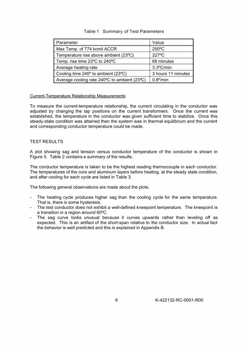
Table 1 Summary of Test Parameters

Parameter Value

Max Temp. of 774 kcmil ACCR 250ºC

Temperature rise above ambient (23ºC) 227ºC

Temp. rise time 23ºC to 240ºC 68 minutes Average heating rate 3.3ºC/min

Cooling time 240º to ambient (23ºC) 3 hours 11 minutes

Average cooling rate 240ºC to ambient (23ºC) 0.8º/min

Current-Temperature Relationship Measurements

To measure the current-temperature relationship, the current circulating in the conductor wasadjusted by changing the tap positions on the current transformers. Once the current wasestablished, the temperature in the conductor was given sufficient time to stabilize. Once this

steady-state condition was attained then the system was in thermal equilibrium and the currentand corresponding conductor temperature could be made.

TEST RESULTS

A plot showing sag and tension versus conductor temperature of the conductor is shown inFigure 5. Table 2 contains a summary of the results.

The conductor temperature is taken to be the highest reading thermocouple in each conductor.The temperatures of the core and aluminum layers before heating, at the steady state condition,and after cooling for each cycle are listed in Table 3.

The following general observations are made about the plots.

- The heating cycle produces higher sag than the cooling cycle for the same temperature.That is, there is some hysteresis.

- The test conductor does not exhibit a well-defined kneepoint temperature. The kneepoint isa transition in a region around 60ºC.

- The sag curve looks unusual because it curves upwards rather than leveling off asexpected. This is an artifact of the short-span relative to the conductor size. In actual factthe behavior is well predicted and this is explained in Appendix B.

6 K-422132-RC-0001-R00



Sag and Tension vs. Temperature

20% RTS Starting Tension

0

2000

4000

6000

8000

10000

12000

14000

16000

0 50 100 150 200 250 300

Temperature, degrees C

T e n s i o n ,

l b F

0

5

10

15

20

S a g ,

i n

Tension

SagHeating

Cooling

Heating

Cooling

Figure 5 Conductor Sag and Tension vs. Temperature

Table 2 Summary of High Temperature Test Results

23ºC

(Before Heating)250ºC Net Change

Sag1.9 inch

(48mm)

18.0 inch

(457 mm)

16.1 inch

(409 mm)

Tension14251 lbf

(6464 kg)

1506 lbf

(583 kg)

12745 lbf

(5781 kg)

Tension(%RBS)

20% 2.1% 17.9%

7 K-422132-RC-0001-R00



Table 3 Temperatures of Core and Aluminum Layers

Core BetweenCore-InnerLayer

BetweenTwo Innerlayerstrands

Betweentwo Outerlayerstrands

Before heating 23 23 23 23

At steady state 250 252 251 245

After cooling 23 22 23 23

Analysis

Data was analyzed by Dr. Stephen Barrett of Barrett Research to look at how the data comparesto predictions from transmission line design software such as Sag10TM software and STESS(Strain Summation method). Both calculate sag using the Alcoa graphical method. Theseanalyses are shown in Appendix B and were performed independently of Kinectrics Inc. The“compressive stress parameter” or “built-in tensile stress parameter” should be set at –1.45 ksi (-10 MPa) for the line design software programs.

Current-Temperature Relationship Measurements

Seven (7) different currents were circulated through the conductor. They were 1630 A , 1502 A,1290 A, 1070 A, 700 A, 564 A, and 420 A.

The corresponding steady-state conductor temperatures, including the condition at 250C, areshown in the following table.

Steady-State CurrentSteady-State Conductor

Temperature

1630 2521502 210

1290 165

1070 122

700 66

564 49

420 36

A plot showing the steady-state currents versus conductor temperatures are shown in Figure 7.The temperature plotted is the hottest of the measured thermocouples. An exponential curve isfitted through the points.

8 K-422132-RC-0001-R00



0

50

100

150

200

250

300

200 400 600 800 1000 1200 1400 1600 1800

Current, Amps

T e m p e r a t u r e ,

d e g C

Figure 7 Conductor Temperature vs. Circulating Current

The predicted ampacity was supplied by 3M Company using RateKitTM software and selecting theIEEE 738 Transient Ampacity Method. The comparison with the measured data is shown inFigure 8. Since the experiment was performed indoors, the parameters selected for the modelinputs included no solar effects, zero wind speed, and an ambient temperature of 25°C for <1200amps and 35°C for > 1200 amps. There is reasonable agreement between the data and themodel prediction.

9 K-422132-RC-0001-R00



0

100

200

300

0 200 400 600 800 1000 1200 1400 1600 1800

Current, A

T e m p e r a t u r e ,

C

Measured T, C

Computed using 0.3 emissivity

Figure 8 Predicted and Measured Conductor Temperature vs. Circu lating Current

CONCLUSIONS

1. A sag-tension-temperature study on 774 kcmil ACCR showed a knee-point transition in

the range of 60°C.2. The “compressive stress parameter” or “built-in tensile stress parameter” should be set at

–1.45 ksi (-10 MPa) for the line design software programs.3. The line design software programs such as Alcoa Sag10TM software and STESS predict

the sag-tension-temperature behaviour very well.

10 K-422132-RC-0001-R00



Prepared by: __________________________________________________C.J. PonPrincipal Engineer

Transmission and Distribution Technologies Business

Approved by: ___________________________________________________Dr. J. KuffelGeneral ManagerTransmission and Distribution Technologies Business

CJP:JC

ACNOWLEDGEMENTS AND DISCLAIMER

Kinectrics North America Inc. has prepared this report in accordance with, and subject to, the termsand conditions of the contract between Kinectrics North America Inc. and 3M Company, dated

August 9, 2004.

This material is based upon work supported by the U.S. Department of Energy under Award No.DE-FC02-02CH11111. Any opinions, findings, and conclusions or recommendations expressedin this material are those of the author(s) and do not necessarily reflect the views of theDepartment of Energy.

11 K-422132-RC-0001-R00



13 K-422132-RC-0001-R00



APPENDIX B

Report on774 kcmil T53 (46/37) ACCRHeat-Run Tests at Kinectrics

October 1, 2005

Prepared by:Stephen Barrett, Barrett Research

Barrett Research, 93 Thomas Blvd. SS3 Elora, Ont. Canada NOB [email protected]

14 K-422132-RC-0001-R00



774 kcmil T53 (46/37) ACCRTested by Kinectr ics on September 14, 2005

Analysis by Barret t Research, October 1, 2005

Introduction

Kinectrics tested a 123 ft. span of 774 kcmil T53 (46/37) ACCR (Rated Tensile Strength =

71,010 lbf), which has a large core for river-crossing purposes. The tension was 14,251 lb (20%

RTS) @ 23.7°C at the start of the test at 14:13 on September 14, 2005.

Because the span is so short, the weight and length of the dead-ends and any small “poledeflection”. has a large effect on sags and tensions. For this reason, Kinectrics used string

transducers to measure the varying span length throughout the test. The vertical displacements

were also measured at mid-span and at the mouths of the two dead-ends, so that the sag

contribution from drooping dead-ends could be removed from the test. The measured sag wasequal to the mid-span height minus the average of the heights at the mouths of the dead-ends.This sag was found to be in good agreement with sag computed from the tension.

A fit to the rising-temperature curve has been added to Kinectric’s graph of span length:

Data from Pull-wire Transduc ers at Deadends

20% RTS Starting Tension

122.99

123

123.01

123.02

123.03

123.04

123.05

123.06

1000 3000 5000 7000 9000 11000 13000 15000 17000

Tension, lbs

S p a n

L e n

g t h ,

f e e t B - B (

F i g

1 )

Measured Span Length

Fit

15 K-422132-RC-0001-R00



The fit is described by:

H H

Span6

21075.1

000,60025.123 −

×−+=

where span is in feet and tension H is in lbf. The first term is caused by the droop of the dead-ends at high temperatures (low tensions) and the second term is a small but significant elastic

deflection in the end hardware.

The following graph is Kinectrics’ graph of tension and sag vs temperature. Temperature is the

maximum of six thermocouples, which turns out to be the core temperature. The model

calculations were performed for both a fixed span (dashed lines) and a span varying according tothe equation above. The default compressive load of –1.45 ksi (-19 MPa) was used. Stress-

strain and creep properties of the core and aluminum were taken to be the same as 3M’s 1272

kcmil ACCR. Sag tension calculations were performed using STR4 (Version 4 of the Strain-

Summation Method, a descendant of STESS).

Sag and Tension vs. Temperature

20% RTS Starting Tensi on

0

2000

4000

6000

8000

10000

12000

14000

16000

0 50 100 150 200 250 300

Temperature, degrees C

T e n s i o n ,

l b F

0

5

10

15

20

25

S a g ,

i n

Measured TensionModel Tension - Fixed Span -1.45 ksiModel Tension - Varying Span -1.45 ksiMeasured SagModel Sag - Fixed Span -1.45 ksiModel Sag - Varying Span -1.45 ksi

Tensio

Sa

Heating

Cooling

Heating

Cooling

16 K-422132-RC-0001-R00



Results The model calculations are in good agreement with the measured values of tensions and sags forrising temperature. (The variation of span was fitted to the rising-temperature span-length curve

in the previous graph.)

The sag curves look unusual because they curve upwards rather than levelling off as expected.The reason is that the span length is very short, which produces a flat catenary, which, in turn,

leads to a concave-upwards shape of the sag-temperature curve. For longer spans, this concavity

is limited to the lower portion of the curve. The concavity is caused by elastic contraction of theconductor as the tension drops. This contraction counteracts part of the thermal elongation. The

counteracting effect is greater at low temperatures where the rate of change of tension is highest.

The concave upward shape can mask the knee-point which can be seen in the model curves at

approximately 60°C. The knee-point is not very visible in the measured curves because

variability of tension in the aluminum wires tends to smooth out the knee-point.

Conclusions

The behaviour of the conductor is very close to what the model predicts. The model has not been “fitted” to the measured curve. Its predictions are based only on the usual material properties of the ACCR materials, using the default value of compressive aluminum stress. The

effect of the latter is small in any case because of the large core. The only other inputs were the

starting temperature and tension and the measured variability of span length. For long spans, theappearance of the sag-temperature graph will have a more normal appearance and corrections for

variation of span length are not normally required. The test was very well executed and there is

no need to repeat it.

17 K-422132-RC-0001-R00



DISTRIBUTION

Dr. Colin McCullough (2) 3M CompanyComposite Conductor Program2465 Lexington Ave. SouthMendota Heights, MN55120USA

Mr. C. Pon Kinectrics Inc., KB104

18 K-422132-RC-0001-R00

774 kcmil accr sag and amp

Documents