7 oktober 2009

Challenge the future

DelftUniversity ofTechnology

Modelling the Climate“a modelling perspective on climate change”

Part 2 AE4-E40 Climate Change

A. Pier SiebesmaKNMI & TU DelftMultiscale Physics DepartmentThe NetherlandsContact: siebesma@knmi.nl

2Climate modeling

Previous Lecture

• Simple Energy Balance Models (0-dimensional models)

• Concept of Radiative Forcing (1-dimensional models)

• How to “translate” this in a temperature change in a static climate

• Architecture of climate models (3-dimensional models)

Today

• Model Predictability

• Model Skill

• Model Sensitivity

• Future Climate Scenario’s (Global and Regional)

3Climate modeling

1.Predictability

4Climate modeling

Ed Lorenz (1918-2008)

Founder of ”the chaos theory”

Predictability for weather forecasting

Toy model for weather: Lorenz-model

5Climate modeling

Two time series for the x-component from nearly identical initial conditions

6Climate modeling

Does the flap of a butterfly’s wings in Brazil set off a tornado in Texas? Lorenz (1972)

x

yThe butterfly effect is the sensitive dependence on initial conditions, where a small difference in initial conditions in a deterministic nonlinear system results large differences to a later state.

7Climate modeling

Ensemble prediction in the Lorenz Attractor

UK MetOffice

8Climate modeling

Ensemble prediction in a operational Weather Forecast Model

9Climate modeling

Ensemble Prediction for the Bilt

from WEdnesday January 9

10Climate modeling

Ensemble Prediction for the Bilt

from Thursday

January 10

11Climate modeling

Remarks

• Predictability horizon for “weather” is now between 5 and 15 days (dependent on the initial state)

• Predictability horizon can be extended through • More accurate estimate of the initial state (more observations)• Improved model formulation (resolution and parameterizations)

• Error growth in non-linear systems is exponential. It becomes therefore increasingly more difficult to extend the predictability horizon.

12Climate modeling

Question

Can we make any reliable statements on changes in weather and climate on time scales beyond 15 days? (seasonal, decadal, century ………)

Free after often received complaints at KNMI:

“ Why are those assholes at KNMI waisting our money on climate predictions if they cannot even predict the weather of tomorrow”

13Climate modeling

Hint

Weather (atmospheric) prediction is essentially a initial value problem:

timescale boundary conditions >> timescale prediction period (15 days)e.g. Continents, Glaciers, Atmospheric Composition, vegetation, solar constant, ocean temperatures can be kept constant!

Atmosphere loses its “memory” after two weeks – any predictability beyond two weeks residing in initial values must arise from predictability from slowly varying boundary conditions

14Climate modeling

Long lasting sea surface temperature (SST) anomalies: El Nino

On timescales ofseasons to years:

15Climate modeling

….. and is influencing the precipitation

16Climate modeling

El Niño Teleconnections

But only at certain areas in the world……..

17Climate modelingTAC 42 Verification 2010

Seasonal forecast – Nino SST, annual range

EUROSIP forecasts of SST anomalies over the NINO 3.4 region of the tropical Pacific from July 2009, December 2009 and May 2010. Showing the individual ensemble members (red); and the subsequent verification (blue)

18Climate modeling

Predictions at a seasonal scale

• Extension beyond the 15 days predictability horizon is possible through the thermal inertia of oceans, snow, soil

• Requires coupling of the atmosphere with the ocean (which is the most important source of inertia)

• So far only “somewhat” successful in the tropics. Outside the tropics the coupling between atmosphere and ocean is weak. In Europe there is little skill on the seasonal scale*

• Note that the problem is slowly shifting from a initial value problem (weather prediction) to a boundary condition (climate prediction) problem

*therefore any seasonal numerical prediction of a horror winter in Europe does not have any skill.

19Climate modeling

Two types of predictions• Edward N. Lorenz (1917–

2008)

• Predictions of the 1st kind• Initial-value problem• Weather forecasting• Lorenz: Weather forecasting

fundamentally limited to about 2 weeks

• Predictions of the 2nd kind• Boundary-value problem• IPCC climate projections

(century-timescale)• No statements about individual

weather events• Initial values considered

unimportant; not defined from observed climate state

20Climate modeling

Climate “Predictions”

• decadal (10yrs) to centennial is possible through changes of the boundary conditions of the atmosphere:

•through the ocean (1 to 10 year),

•through change in greenhouse gases (10+ years)

21Climate modeling

2.Example : The Challenge Project

22Climate modeling

1900 1940 2000 2080Historical concentrations of Greenhouse gases, sulphate, aerosols, solar variations and vulcanic aerosols

Greenhouse gases according to a‘Business-as-usual’ (BAU) scenario

62 simulatiesStochastic perturbations in temperature (<0.1%)

Dutch Challenge Project

“Simulate with one global climate model the “Earth’s Climate” a large number of times with small perturbations in the initial conditions”

www.knmi.nl/research/CKO/Challenge

23Climate modeling

Variations in Solar Constant

External Forcings

24Climate modeling

Variations in Natural Aerosols: Vulcanic Eruptions

External Forcings

Pinatubo (1991), Filipijnen

El Chichón (1982), Mexico

Agung (1963), IndonesiëSanta Maria (1902), Guatemala

Novarupta (1912), Alaska

25Climate modeling

Variations in Greenhouse Gases

External Forcings

26Climate modeling

Start of the development of the temperature in de Bilt

Atmosphere slowly “forgets” its initial state

Limited predictability of weather

An ensemble of developments of the climate sytem

27Climate modeling

World Averaged Annual Temperature

observed

Model average

28Climate modeling

Winter temperatures in the Netherlands

•Larger variations on a smaller scale

•Cold winters will still happen in the 21st century but the probability gets increasingly smaller

29Climate modeling

3.Skill of Climate and Weather

Models

30Climate modeling

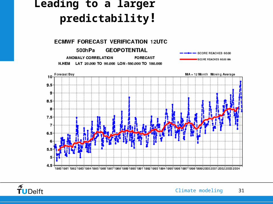
Skill of Weather Prediction Models (ECMWF)

Improvement of weather predictions through: • model (processes, resolution

• initialisations (satellites)

Predictive skill >60%

31Climate modeling

Leading to a larger predictability!

ECMWF DA/SAT Training Course, May 2010 32

Significant increase in number of observations assimilated

Conventional and satellite data assimilated at ECMWF 1996-2010

33Climate modeling

But what is the skill of a Climate Model?

or

How well do climate models simulate today’s climate?

34Climate modeling

No commonly accepted skill metrics for climate models yet because:

• Unlike for weather prediction models a limited set of observables (pressure fields) may not be sufficient.

• Opportunities to test climate model skills is limited

• Lack of reliable and consistent observations for present climate

A skill metrics would be desirable because:

• To objectively measure progress in climate model development

• To be able to set a standard for climate models that can participate in future climate model scenario’s such as for IPCC

35Climate modeling

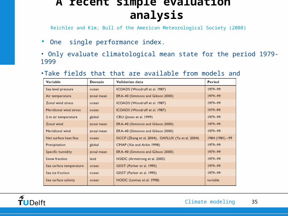
A recent simple evaluation analysisReichler and Kim; Bull of the American Meteorological Society (2008)

• One single performance index.

• Only evaluate climatological mean state for the period 1979-1999

•Take fields that that are available from models and observations

36Climate modeling

Model output from 3 different climate model intercomparison projects (CMIPS)

•CMIP1 : 18 different climate models (1995)

•CMIP2 : 17 different climate models (2003)

•CMIP3 : 22 different climate models (2007)

Method

Normalized error variance for each variable v for model m:

Rescale e2 by the average error found in the CMIP3 ensemble:

Take the mean over all climate variables:

37Climate modeling

Results of Performance index I

Best performing models have low I

Grey circles indicate the average I of a model group

Black circles indicate multimodel mean

Take home messages: •Improvement of climate models over the years

•Multimodel mean outperforms any single model

38Climate modeling

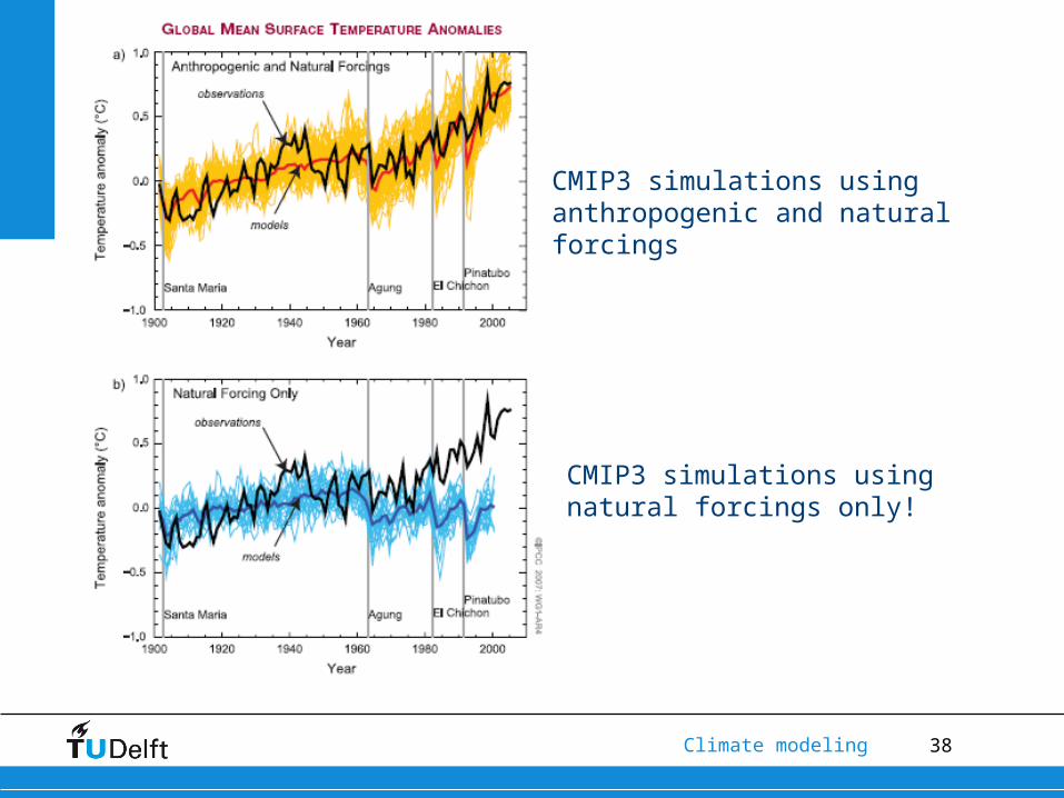
CMIP3 simulations using anthropogenic and natural forcings

CMIP3 simulations using natural forcings only!

39Climate modeling

Same picture for regional trends

40Climate modeling

4.Climate Model Sensitivity:

41Climate modeling

Uncertainties in Future Climate model Predictions with different climate

models

2.5-4.3°CIPCC 2007

Past FuturePresent190

0

42Climate modeling

Climate Model Sensitivity

temperature radiative forcing

Water vapour

With feedbacks:

Snow albedo

clouds

43Climate modeling

Dufresne & Bony, Journal of Climate 2008

Radiative effects only

Water vapor feedback

Surface albedo feedback

Cloud feedback

Cloud effects “remain the largest source of uncertainty”in model based estimates of climate sensitivity IPCC 2007

2XCO2 Scenario for 12 Climate Models

44Climate Modelling

Primarily due to marine low clouds

“Marine boundary layer clouds are at the heart of tropical cloud feedback uncertainties in climate models”

(duFresne&Bony 2005 GRL)

Stratocumulus

Shallow cumulus

45Climate Modelling

• Definition: temperature change resulting from a perturbation of 1 Wm -2

• Radiative forcing for 2XCO2 3.7 Wm-2 (R)

• Temperature response of climate models for 2XCO2 2~4.3 K (T)

• Climate model sensitivity: 0.5-1.2 K per Wm-2 (T/R)

• The climate model sensitivity is not (very) dependent on the source of the perturbation (radiative forcing)

• Main reason for this uncertainty are the representation of (low) clouds

• Reducing uncertainty of climate models can only be achieved through a more realistic representation of cloud processes and is one of the major challenges of climate modelling

Climate Model Sensitivity

46Climate modeling

5.Future Global Climate Scenario’s

47Climate modeling

Emission scenarios from IPCC, includes also air pollution giving aerosols

ppm

EXPERIMENT TYPES

48Climate modeling

Projections of global temperature change

Source : IPCC

+2K

49Climate modeling

IPCC 2007

50Climate modeling

Projections for surface temperatures

51Climate modeling

Future seasonal mean Precipitation Changes

“the wet get wetter and the dry get dryer”

52Climate modeling

Remarks

• Increase of precipitation at high latitudes

• Decrease of precipitation at the subtropical land regions

• Due to increased transport of water vapour from the lower latitudes poleward.

• Note that Netherlands is on the borderline.

53Climate modeling

6.Future Regional Climate Scenario’s

54Climate modeling

Global Climate Models have their limitations

GCMs have a coarse resolution (150~300 km)

• Land-sea mask• Topography• Convection, clouds, precipitation• Land atmosphere interaction

RCM

GCM

How can we increase the resolution ?

55Climate modeling

Dynamical downscaling with regional climate

models (RCMs)

•RCMs “are” GCMs, but:• higher resolution (10km)• limited domain

• Purpose: Better local representation

• RCM needs to be feeded at the boundaries with data from a GCM

•Acts like a looking glass.

•But….. which GCM should be used for downscaling????

56Climate modeling

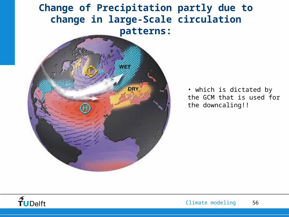
Change of Precipitation partly due to change in large-Scale circulation patterns:

• which is dictated by the GCM that is used for the downcaling!!

57Climate modeling

1 RCM with 2 GCM (boundaries)

GC

M1

GC

M2

58Climate modeling

4 scenario’s for the Netherlands

Gematigd+verandering

+ 1 °C + 2 °C

Luchtstromingspatronen

WereldTemperatuur

Warm+verandering

Gematigd Warm

gew

ijzig

do

ng

ewijz

igd

in 2050 t.o.v. 1990

59Climate modeling

KNMI 2007 Scenario’s

http://www.knmi.nl/klimaatscenarios/

Winter precip increases, also extremes.

Summer precip decreases (probably); increase extremes

60Verstoorde wolken in een opwarmend klimaat

Fractional Uncertainty for future global climate (%)

2000 2100Time

Model uncertainty (e.g. clouds)

Scenario uncertainty (Societal)

Internal Variability (Ocean Initialisation)

Hawkins and Sutton (2009)

61Climate modeling

The Road Ahead……..

• Better Observations (initialisation, monitoring, evaluation)

• Better Models ( Through process studies of relevant process studies e.g. clouds)

• Emissions : Couple Carbon cycle with GCM’s but ultimately this remains a societal and ethical problem (economics, politics)

62Climate modeling

Examples of Questions1 a) Describe the greenhouse effect.1b) Describe how the greenhouse effect is affected by increase of CO2

3) What are the main components that are needed in a 3-dimensional climate model. Explain why they are necessary

4) What are parameterizations? Why do they need to be included in climate models. What would happen if you would run a climate model without parameterizations of clouds.

5) Explain the concept of radiative forcing. Which are the main contributors. Which ones are the source of the largest uncertainties in the radiative forcing.

6) What defines the predictability of a numerical weather model. Why is it possible that we can still make climate model predictions on much longer timescales? Discuss the differences.

7) What is climate model sensitivity? Which are the most important sources for uncertainty in climate model sensitivity? Explain why.

8) How are regional climate models used for future climate scenario’s?

Describes the pro’s and con’s