7. multirate dsp - weebly · dsp-7 (multirate) 1 of 58 dr. ravi billa digital signal processing –...
TRANSCRIPT

DSP-7 (Multirate) 1 of 58 Dr. Ravi Billa
Digital Signal Processing – 7 November 16, 2009
7. Multirate DSP
(Deleted in 2007 Syllabus).
2007 Syllabus: Decimation, Interpolation, Sampling rate conversion, Filter design and
Implementation of sampling rate conversion.
Contents:
7.1 Time and frequency scaling in continuous-time systems
7.2 Transformation of the independent variable
7.3 Down-sampling
7.4 Up-sampling
7.5 Cascading sampling rate converters
7.6 Identities
7.7 FIR implementation of sampling rate conversion
7.8 Polyphase structures
7.9 Polyphase structure for a decimator
Discrete-time systems with different sampling rates at various parts of the system are called
multirate systems. They are linear and time-varying systems. Integer sampling rate converters
change the sampling frequency by an integer factor and rational sampling rate converters by a
rational number. Here is a sampling of sampling rates in commercial applications (Mitra):
Sampling Rates
Digital Audio Video
Broadcasting – 32 kHz
CD – 44.1 kHz
DAT – 48 kHz
Composite Video Signal
NTSC – 14.3181818 MHz
PAL – 17.734475 MHz
Digital Component Video Signal
Luminance – 13.5 MHz
Color difference – 6.75 MHz
www.jntuworld.com
www.jntuworld.com

DSP-7 (Multirate) 2 of 58 Dr. Ravi Billa
7.1 Time and frequency scaling in continuous-time systems
Illustration An audio signal recorded on cassette tape at a certain speed could be played back at
a higher speed than that at which it was recorded. This is called time scaling, in particular,
compression in the time domain, and results in an inverse effect in the frequency domain, i.e., an
expansion of the frequency spectrum. Similarly when the audio signal is played back at a slower
speed than the recording speed we have expansion in the time domain resulting in a
corresponding compression of the spectrum in the frequency domain.
Given the signal x(t) and its Fourier transform X(Ω), represented notationally by
x(t) ↔ X(Ω)
then time scaling results in
x(at) ↔ a
1X(Ω/a)
If a > 1 the scaling corresponds to compression in time. If, for instance, a = 2, we may visualize
a new signal y1(t) = x(2t); with t = 1, for instance, the value of x, that is, x(2) that occurred at 2
seconds occurs at 1 second in the case of y1, that is, y1(1) – which is compression in time.
x(t)
t 1 0
B
A
X(Ω)
Ω C –C 0
x(2t)
0 1/2 t
B
1
X(Ω/2)
Ω C –2C 0 2C
A
B
0 2 1
x(t/2)
t
X(2Ω)
Ω C –C/2 0 C/2
www.jntuworld.com
www.jntuworld.com

DSP-7 (Multirate) 3 of 58 Dr. Ravi Billa
If x(t) is an audio signal recorded on tape then x(2t) could be the signal x(t) played back at twice
the speed at which x(t) was recorded. The signal x(2t) varies more rapidly than x(t) and the
playback frequencies are higher.
If a < 1 the scaling corresponds to expansion in time. If, for instance, a = 1/2, then x(t/2)
is the signal x(t) played back at half the speed at which x(t) was recorded. The signal x(t/2) varies
slower than x(t) and the playback frequencies are lower. Again, we may visualize this as a new
signal y2(t) = x(t/2); the value of x(.) that occurred at t/2 occurs at t in the case of y2(.) – which is
expansion in time.
Time expansion and frequency compression is found in data transmission from space
probes to receiving stations on earth. To reduce the amount of noise superposed on the signal, it
is necessary to keep the bandwidth of the receiver as small as possible. One means of doing this
is to reduce the bandwidth of the signal: store the data collected by the probe, and then transmit it
at a slower rate. Since the time-scaling factor is known, the signal can be reproduced at the
receiver.
The corresponding operations in the case of discrete-time systems are not quite so
straight forward owing to
1. The need to band limit the continuous-time signal prior to sampling, and
2. The need to avoid aliasing in the process of sampling
Example 1.1 Consider the 4 Hz signal x(t) = cos 2π4t which is obviously band-limited to Fmax =
4 Hz. It is sufficient to sample it at 8 Hz. Alternatively, the signal can be sampled at, say, 16 Hz
or 20 Hz etc. Suppose that it has been over-sampled by a factor of, say, 6 at Fs = 48 Hz to give
x(n) = cos 2π4n(1/48) = cos (πn/6).
(a) If it is desired subsequently to generate from x(n) another signal x1(n) that is a
discrete-time version of x(t) sampled at Fs1 = 16 Hz ( sampling rate reduced by a
factor of 3), then can we do this by simply dropping two samples of x(n) for every
sample that we keep? That is x1(n) = x(3n). This is called down-sampling.
(b) How do we generate from x(n) another signal x2(n) that is a discrete-time version of
x(t) sampled at, say, Fs2 = 96 Hz ( sampling rate doubled)? This is called up-
sampling.
(c) Can we generate from x(n) another signal x3(n) that is a discrete-time version of x(t)
sampled at Fs3 = 6 Hz?
We pick up on this problem again after covering transformation of the independent variable.
7.2 Transformation of the independent variable
Time scaling (Refer also to Section 7.5 of Signals and Systems, Oppenheim and Willsky.) Given
the sequence x(n), the sequence y(n) = x(2n) is obtained by skipping odd-numbered samples in
x(n) and retaining the even-numbered ones. The extension to y(n) = x(Mn) means we retain
sample numbers 0, M, 2M, 3M, …, and skip the intervening M–1 samples between those we
keep. The original sequence x(n) is obtained by sampling a continuous signal x(t) at a certain rate
(perhaps over-sampling). The signal y(n) = x(Mn) is then obtained by reducing the sampling rate
by a factor of M on the continuous-time signal x(t). This is known as down-sampling or
decimation or sampling rate compression.
Similarly the process of constructing the sequence y(n) = x(n/L) from the sequence x(n)
means we derive y(n) by inserting (L–1) sequence points with zero value between points of x(n).
This is called up-sampling or interpolation or sampling rate expansion. (Inserting (L–1) zeros is
www.jntuworld.com
www.jntuworld.com

DSP-7 (Multirate) 4 of 58 Dr. Ravi Billa
just one way of interpolating. It is also possible for the up-sampler to be followed by a digital
system that replaces the inserted zeros with more appropriate values based on a linear
combination of the x(n) samples.)
In general, the result of time scaling a discrete-time signal is not just a stretched or
compressed version of the original but possibly a totally different sequence/waveform.
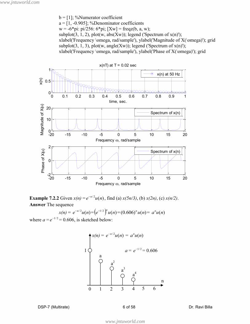
Example 7.2.1 Given that x(t) = )(5 tue t is sampled at 50 Hz, find an expression for x(n). Plot
x(t), x(n) and x(2n). Sketch the spectrum of x(n).
Solution The sampling time is T = 0.02 sec. Replacing t with nT we get x(nT) = )(5 nTue nT , or
x(n) = )(1.0 nuen = )()905.0( nun .
We show below three plots: (1) The continuous-time signal x(t), (2) The sampled (at 50 Hz)
version x(n), and (3) x(2n), the 2-fold down-sampled version of x(n); this is equivalent to
sampling x(t) at 25 Hz.
t = 0 : 1/512: 1; xt = exp (-5*t); %x(t) evaluated at 512 points
subplot(3, 1, 1), plot(t, xt); legend ('x(t) = exp(-5t)');
xlabel ('time, sec.'), ylabel('x(t)'); grid; title ('x(t) – Continuous-time')
%
t1 = 0 : 0.02: 1; xn = exp (-5*t1); %Sampled at 50 Hz.
subplot(3, 1, 2), stem(t1, xn); legend ('x(n) at 50 Hz');
xlabel ('time, sec.'), ylabel('x(n)'); grid; title ('x(nT) at T = 0.02 sec')
%
t2 = 0 : 0.04: 1; xt2 = exp (-5*t2); %Sampled at 25 Hz
subplot(3, 1, 3), stem(t2, xt2); legend ('2-fold down-sampled');
xlabel ('time, sec.'), ylabel('x(2n)'); grid; title ('x(nT) at T = 0.04 sec.')
0 0.1 0.2 0.3 0.4 0.5 0.6 0.7 0.8 0.9 10
0.5
1
time, sec.
x(t
)
x(t) – Continuous-time
x(t) = exp(-5t)
0 0.1 0.2 0.3 0.4 0.5 0.6 0.7 0.8 0.9 10
0.5
1
time, sec.
x(n
)
x(nT) at T = 0.02 sec
x(n) at 50 Hz
0 0.1 0.2 0.3 0.4 0.5 0.6 0.7 0.8 0.9 10
0.5
1
time, sec.
x(2
n)
x(nT) at T = 0.04 sec.
2-fold down-sampled
www.jntuworld.com
www.jntuworld.com

DSP-7 (Multirate) 5 of 58 Dr. Ravi Billa
Note that X(s) = ℒ )(5 tue t = )5(1 s . Shown below is the MATLAB plot of the
magnitude spectrum |X(jΩ)| of the continuous-time signal x(t) using the function plot. Omega is a
vector, consequently we use “./” instead of “/” etc. The main point to be made here is that X(jΩ)
extends asymptotically to ∞, so, strictly speaking, x(t) is not band-limited. Consequently, the
spectrum X(ω) of the sampled signal x(n) (shown later below) has some built-in aliasing.
t = 0 : 1/512: 1; xt = exp (-5*t); %x(t) evaluated at 512 points
subplot(3, 1, 1), plot(t, xt); legend ('x(t) = exp(-5t)');
xlabel ('time'), ylabel('x(t)'); grid; title ('x(t) – Continuous-time')
%
Omega = -6*pi: pi/256: 6*pi; X = 1./(5.+ j .*Omega);
subplot(3, 1, 2), plot(Omega, abs(X), 'k'); legend ('Spectrum of x(t)');
xlabel ('Omega, rad/sec'), ylabel('|X(Omega)|'); grid; title ('Magnitude')%
subplot(3, 1, 3), plot(Omega, angle(X), 'k'); legend ('Spectrum of x(t)');
xlabel ('Omega, rad/sec'), ylabel('Phase of X(Omega)'); grid; title ('Phase')
0 0.1 0.2 0.3 0.4 0.5 0.6 0.7 0.8 0.9 10
0.5
1
time
x(t
)
x(t) – Continuous-time
-20 -15 -10 -5 0 5 10 15 200
0.1
0.2
Omega, rad/sec
|X(O
mega)|
Magnitude
-20 -15 -10 -5 0 5 10 15 20-2
0
2
Omega, rad/sec
Phase o
f X
(Om
ega) Phase
x(t) = exp(-5t)
Spectrum of x(t)
Spectrum of x(t)
Coming to the discrete-time signal, the spectrum of x(n) = )(nuan = )()905.0( nun is its
DTFT
)( jeX =
0n
njn ea =
jea 1
1 =
je 905.01
1
The MATLAB segment is
t1 = 0 : 0.02: 1; xn = exp (-5*t1); %Sampled at 50 Hz.
subplot(3, 1, 1), stem(t1, xn); legend ('x(n) at 50 Hz');
xlabel ('time, sec.'), ylabel('x(n)'); grid; title ('x(nT) at T = 0.02 sec')
%
www.jntuworld.com
www.jntuworld.com
DSP-7 (Multirate) 6 of 58 Dr. Ravi Billa
b = [1]; %Numerator coefficient
a = [1, -0.905]; %Denominator coefficients
w = -6*pi: pi/256: 6*pi; [Xw] = freqz(b, a, w);
subplot(3, 1, 2), plot(w, abs(Xw)); legend ('Spectrum of x(n)');
xlabel('Frequency \omega, rad/sample'), ylabel('Magnitude of X(\omega)'); grid
subplot(3, 1, 3), plot(w, angle(Xw)); legend ('Spectrum of x(n)');
xlabel('Frequency \omega, rad/sample'), ylabel('Phase of X(\omega)'); grid
0 0.1 0.2 0.3 0.4 0.5 0.6 0.7 0.8 0.9 10
0.5
1
time, sec.
x(n
)
x(nT) at T = 0.02 sec
-20 -15 -10 -5 0 5 10 15 200
10
20
Frequency , rad/sample
Magnitude o
f X
()
-20 -15 -10 -5 0 5 10 15 20-2
0
2
Frequency , rad/sample
Phase o
f X
()
x(n) at 50 Hz
Spectrum of x(n)
Spectrum of x(n)
Example 7.2.2 Given x(n) = )(2/ nue n , find (a) x(5n/3), (b) x(2n), (c) x(n/2).
Answer The sequence
x(n) = )(2/ nue n = )(2/1 nuen = )()606.0( nun = )(nuan
where a = 2/1e = 0.606, is sketched below:
0 1 2 3 4 5 6
x(n) = )(2/ nue n = )(nuan
n
1
a2
a3
a4
a a = 2/1e = 0.606
www.jntuworld.com
www.jntuworld.com

DSP-7 (Multirate) 7 of 58 Dr. Ravi Billa
(a) With y(n) = x(5n/3), we evaluate y(n) for several values of n (we have assumed here that x(n)
is zero if n is not an integer):
y(0) = x(5 . 0/ 3) = x(0) = 2/0e = 1
y(1) = x(5 . 1/ 3) = x(5 / 3) = 0
y(2) = x(5 . 2/ 3) = x(10 / 3) = 0
y(3) = x(5 . 3/ 3) = x(5) = 2/5e = 5a
…
y(6) = x(5 . 6 / 3) = x(10) = 2/10e = 10a
…
The general expression for y(n) can be written as
y(n) = x(5n/3) = 2/)3/5( ne , n as specified below
= 6/5ne , n = 0, 3, 6, …
0, otherwise
n = 0 1 2 3 4 5 6 7 8 9 10
y(n) = 1 0 0 a5 0 0 a
10 0 0 a
15 0
The sequence is sketched below:
(b) With y(n) = x(2n), we evaluate y(.) for several values of n:
y(0) = x(2 . 0) = x(0) = 1
y(1) = x(2 . 1) = x(2) = a2
y(2) = x(2 . 2) = x(4) = a4
y(3) = x(2 . 3) = x(6) = a6
…
The general expression for y(n) can be written as
y(n) = x(2n) = e–(2n)/2
, n as specified below
= e–n
, n ≥ 0
0, otherwise
0 1 2 3 4 5 6
y(n) = x(5n/3) = e–5n/ 6
, n = 0, 3, 6, …
0, otherwise
n
1
a5
a10
a = e–1/ 2
= 0.606
www.jntuworld.com
www.jntuworld.com

DSP-7 (Multirate) 8 of 58 Dr. Ravi Billa
n = 0 1 2 3 4 5
y(n) = 1 a2
a4
a6 a
8 a
10
The sequence y(.) is made up of every other sample of x(.). This is down-sampling or
decimation by a factor of 2 (or, compression in time). Note that some of the original sample
values have disappeared. The sequence is sketched below.
(c) With y(n) = x(n/2) = )(4/ nue n , we evaluate y(.) for several values of n (again, we have
assumed here that x(n) is zero if n is not an integer):
y(0) = x(0/2) = x(0) = 1
y(1) = x(1/2) = x(0.5) = 0
y(2) = x(2/2) = x(1) = a
y(3) = x(3/2) = x(1.5) = 0
…
The general expression for y(n) can be written as
y(n) = x(n/2) = e–(n/2)/2
, n as specified below
= e–n/ 4
, n = 0, 2, 4, …
0, otherwise
n = 0 1 2 3 4 5 6
y(n) = 1 0
a
0 a2 0 a
3
The sequence y(.) is constructed by inserting one zero between successive samples of x(.). This is
up-sampling or interpolation by a factor of 2 (or expansion in time). The sequence is sketched
below:
0 1 2 3 4 5 6
n
1
a2
a4
a = e–1/ 2
= 0.606
a6
a8
x(n) = e–n
n ≥ 0
0, otherwise
0 1 2 3 4 5 6
n
1
a2
a = e–1/ 2
= 0.606
a3
x(n) = e–n/ 4
n = 0, 2, …
0, otherwise
a
www.jntuworld.com
www.jntuworld.com
DSP-7 (Multirate) 9 of 58 Dr. Ravi Billa
To get back to the problem raised earlier, given the sequence x(n) obtained from x(t) at a
rate (1/T)
x(t) → x(nT) → x(n), rate (1/T)
we want to obtain the sequence )(nx which corresponds to a sampling rate (1/T ) where T ≠T
x(t) → x(nT ) → )(nx , rate (1/T )
There are two approaches to do this:
1. Convert x(n) to x(t) and resample at (1/T ) to generate )(nx . This is not ideal
because of the imperfections in the A/D-H(z)-D/A originally involved in
generating x(n). Or,
2. Change the sampling rate entirely with discrete-time operations.
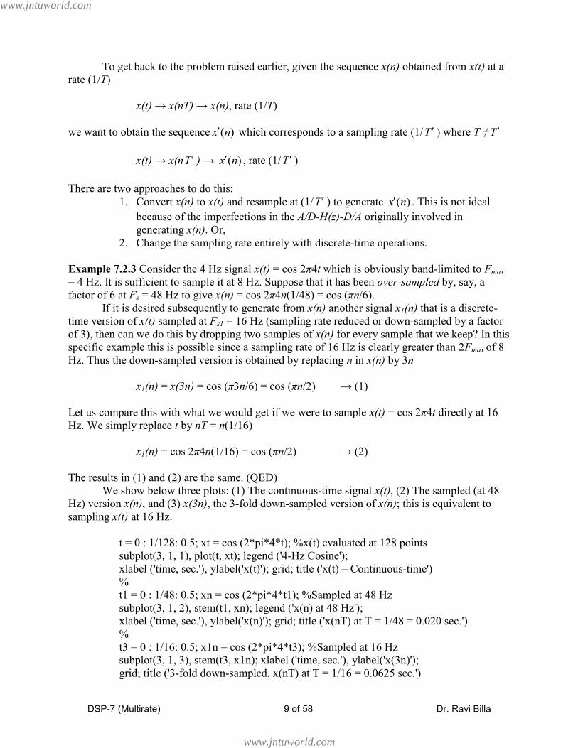
Example 7.2.3 Consider the 4 Hz signal x(t) = cos 2π4t which is obviously band-limited to Fmax
= 4 Hz. It is sufficient to sample it at 8 Hz. Suppose that it has been over-sampled by, say, a
factor of 6 at Fs = 48 Hz to give x(n) = cos 2π4n(1/48) = cos (πn/6).
If it is desired subsequently to generate from x(n) another signal x1(n) that is a discrete-
time version of x(t) sampled at Fs1 = 16 Hz (sampling rate reduced or down-sampled by a factor
of 3), then can we do this by dropping two samples of x(n) for every sample that we keep? In this
specific example this is possible since a sampling rate of 16 Hz is clearly greater than 2Fmax of 8
Hz. Thus the down-sampled version is obtained by replacing n in x(n) by 3n
x1(n) = x(3n) = cos (π3n/6) = cos (πn/2) → (1)
Let us compare this with what we would get if we were to sample x(t) = cos 2π4t directly at 16
Hz. We simply replace t by nT = n(1/16)
x1(n) = cos 2π4n(1/16) = cos (πn/2) → (2)
The results in (1) and (2) are the same. (QED)
We show below three plots: (1) The continuous-time signal x(t), (2) The sampled (at 48
Hz) version x(n), and (3) x(3n), the 3-fold down-sampled version of x(n); this is equivalent to
sampling x(t) at 16 Hz.
t = 0 : 1/128: 0.5; xt = cos (2*pi*4*t); %x(t) evaluated at 128 points
subplot(3, 1, 1), plot(t, xt); legend ('4-Hz Cosine');
xlabel ('time, sec.'), ylabel('x(t)'); grid; title ('x(t) – Continuous-time')
%
t1 = 0 : 1/48: 0.5; xn = cos (2*pi*4*t1); %Sampled at 48 Hz
subplot(3, 1, 2), stem(t1, xn); legend ('x(n) at 48 Hz');
xlabel ('time, sec.'), ylabel('x(n)'); grid; title ('x(nT) at T = 1/48 = 0.020 sec.')
%
t3 = 0 : 1/16: 0.5; x1n = cos (2*pi*4*t3); %Sampled at 16 Hz
subplot(3, 1, 3), stem(t3, x1n); xlabel ('time, sec.'), ylabel('x(3n)');
grid; title ('3-fold down-sampled, x(nT) at T = 1/16 = 0.0625 sec.')
www.jntuworld.com
www.jntuworld.com

DSP-7 (Multirate) 10 of 58 Dr. Ravi Billa
0 0.05 0.1 0.15 0.2 0.25 0.3 0.35 0.4 0.45 0.5-1
0
1
time, sec.
x(t
)
x(t) – Continuous-time
0 0.05 0.1 0.15 0.2 0.25 0.3 0.35 0.4 0.45 0.5-1
0
1
time, sec.
x(n
)
x(nT) at T = 1/48 = 0.020 sec.
0 0.05 0.1 0.15 0.2 0.25 0.3 0.35 0.4 0.45 0.5-1
0
1
time, sec.
x(3
n)
3-fold down-sampled, x(nT) at T = 1/16 = 0.0625 sec.
4-Hz Cosine
x(n) at 48 Hz
Alternatively, assuming x(t) is not available, x1(n) could be obtained as follows:
1. Recover x(t) by passing x(n) through a DAC
2. Sample the resulting x(t) at Fs1 = 16 Hz
We take it, however, that this option is not desirable.
The above analysis assumes that we know the frequency content of the base band signal,
x(t). Generally this is not the case. Given the sequence x(n) that was obtained by sampling at a
rate, say Fs, we do not know what is the maximum frequency, Fmax, contained in the underlying
analog signal, x(t). Assuming it was originally band-limited and properly sampled, it is safest to
assume that the base band signal was band-limited to Fs/2 (= Fmax) and not lower. In such a case
simply dropping one or more samples of x(n) for every sample we keep will not work. If we
want to reduce the sampling rate by a factor of, say, K, then we would have to band-limit the
precursor of x(n) to (Fs/2)/K = (Fs/2K) and then sample it at the K-fold reduced sampling rate to
achieve the required decimation. This amounts to down sampling x(n) by a factor of K. (If the
signal x(t) originally actually contained a maximum frequency of Fs/2 then subsequent down
sampling will result in unavoidable loss of information. But if it was band limited to significantly
less than Fs/2 then down-sampling without loss of information is possible.)
The band-limiting mentioned above may be done either in the continuous-time domain or
in the discrete-time domain. The procedure in the continuous time domain is as follows: Imagine
that x(t) is recovered from x(n); x(t) is then band-limited to Fs/2K by passing it through an ideal
low pass filter described by
H(F) = 1, 0 ≤ F < Fs/2K
0, Fs/2K ≤ F ≤ Fs/2
www.jntuworld.com
www.jntuworld.com

DSP-7 (Multirate) 11 of 58 Dr. Ravi Billa
The band-limited signal, denoted x1(t) is then sampled at the reduced rate of Fs/K to generate
x1(n). This method is generally undesirable because of all the imperfections inherent in originally
generating x(n) from x(t) at a sampling rate of Fs, converting x(n) back into x(t), then band-
limiting x(t) to Fs/2K to generate x1(t) and then sampling x1(t) at a sampling rate of Fs/K to
generate x1(n).
Sampling rate decimation Reducing the sampling rate by an integer factor in the discrete-time
domain is shown in the following block diagram. The down arrow in ↓K indicates down
sampling by a factor of K. The filter H(z) is a digital anti-aliasing filter whose output v(n) is a
low pass filtered version of x(n).
If the filter H(z) is implemented as a linear phase FIR filter with (M+1) coefficients
specified as {br, r = 0 to M}, (some call it “Mth
order”), then
v(n) =
M
r
r rnxb0
)(
We desire the output y(n) to be a down-sampled version of x(n), that is
y(n) = v(Kn) =
M
r
r rKnxb0
)(
Example 7.2.4 Consider the 4 Hz signal x(t) = cos 2π4t which is obviously band-limited to Fmax
= 4 Hz. It is sufficient to sample it at 8 Hz. Suppose instead that it has been over sampled, say,
by a factor of 6 at Fs = 48 Hz to give x(n) = cos 2π4n(1/48) = cos (πn/6).
Can we generate from x(n) another signal x3(n) that is a discrete-time version of x(t)
sampled at Fs3 = Fs/8 = 6 Hz? This is down sampling by a factor of 8. We simply replace t by nT
= n(1/6) to get
x3(n) = cos 2π4n(1/6) = cos (8πn/6) = x(8n) = {x(0), x(8), x(16), …}
In other words, x3(n) is made up of every 8th
sample of x(n). For every sample value of x(n) we
keep we discard the next 7 samples. We know, however, that a sampling frequency of 6 Hz does
not satisfy the sampling theorem; in this case down sampling has been taken too far.
We show below three plots: (1) The sampled (at 48 Hz) version x(n) – this is repeated
from above, (2) x(2n), the 2-fold down-sampled version of x(n); this is equivalent to sampling
x(t) at 24 Hz, and (3) x(8n), the 8-fold down-sampled version of x(n); this is equivalent to
sampling x(t) at the unacceptably low rate of 6 Hz.
t1 = 0 : 1/48: 0.5; xn = cos (2*pi*4*t1); %Sampled at 48 Hz
subplot(3, 1, 1), stem(t1, xn); legend ('x(n) at 48 Hz');
xlabel ('time, sec.'), ylabel('x(n)'); grid; title ('x(nT) at T = 1/48')
%
t2 = 0 : 1/24: 0.5; xt2 = cos (2*pi*4*t2); %Sampled at 24 Hz
x(n) v(n) y(n)
H(z)
↓K
x(t) x1(t) x1(n)
H(F)
Sampler,
Rate = Fs/K
www.jntuworld.com
www.jntuworld.com

DSP-7 (Multirate) 12 of 58 Dr. Ravi Billa
subplot(3, 1, 2), stem(t2, xt2); xlabel ('time, sec.'), ylabel('x(2n)');
grid; title ('2-fold down-sampled, x(nT) at T = 1/24 sec.')
%
t4 = 0 : 1/6: 0.5; x3n = cos (2*pi*4*t4); %Sampled at 6 Hz
subplot(3, 1, 3), stem(t4, x3n); xlabel ('time, sec.'), ylabel('x(8n)');
grid; title ('8-fold down-sampled, x(nT) at T = 1/6 sec.')
0 0.05 0.1 0.15 0.2 0.25 0.3 0.35 0.4 0.45 0.5-1
0
1
time, sec.
x(n
)
x(nT) at T = 1/48
0 0.05 0.1 0.15 0.2 0.25 0.3 0.35 0.4 0.45 0.5-1
0
1
time, sec.
x(2
n)
2-fold down-sampled, x(nT) at T = 1/24 sec.
0 0.05 0.1 0.15 0.2 0.25 0.3 0.35 0.4 0.45 0.5-1
0
1
time, sec.
x(8
n)
8-fold down-sampled, x(nT) at T = 1/6 sec.
x(n) at 48 Hz
Example 7.2.5 To show visually a case of down sampling that is not satisfactory, consider x4(n)
generated from x(n) by down sampling by a factor of 12, i.e., x4(n) = x(12n). This is also
obtained by sampling at 48/12 = 4 Hz:
x4(n) = x(nT) = cos 2π4n(1/4) = cos (2πn) = cos (12πn/6) = x(12n)
In this case cos (2πn) = 1 for all n, so that
x4(n) = 1 for all n
which has no resemblance to x(n), making it visually obvious that down sampling has been taken
too far. Depending on at what point in the cycle the samples are taken, x4(n) equals a constant
(including 0), for all n.
7.3 Down-sampling
www.jntuworld.com
www.jntuworld.com

DSP-7 (Multirate) 13 of 58 Dr. Ravi Billa
Assume that x(n) is obtained from an underlying continuous-time signal x(t) by sampling at Fx
Hz. Assume that x(t) was originally band limited to Fx/2 Hz. On the digital frequency (ω) scale
this amounts to x(n) being band limited to π.
We now wish to generate a signal y(n) by down-sampling x(n) by a factor of M, that is,
we are reducing the sampling rate by a factor of M. This amounts to:
1. Converting x(n) to x(t) using a D/A converter.
2. Band limiting x(t) to Fx/2M Hz. Assume that no information is lost due to this
band limiting.
3. Resampling x(t) at Fx/M Hz. to produce y(n).
Equivalently the above task is accomplished entirely in the digital domain by
1. Band limiting x(n) to π/M. Assume that no information is lost due to this step.
2. Down-sampling the above x(n) by a factor of M to produce y(n).
We may view y(n) as though it were generated by sampling an underlying analog signal y(t) at a
rate Fy = Fx/M Hz. Given the signal x(n) that was obtained at a certain sampling rate the new signal y(n), the
down-sampled version of x(n), with a sampling rate that is (1/M) of that of x(n), obtained from
x(n), is given by:
y(n) = x(Mn)
and is made up of every Mth
sample value of x(n); the intervening (M–1) sample values of x(n)
are dropped. This amounts to
y(0) = x(0), y(1) = x(M), y(2) = x(2M), y(3) = x(3M), …
The time between samples of y(.) is M times that between samples of x(.), or the sampling
frequency of y(.) is reduced by a factor of M from that of x(.). The block diagram of a down
sampler is shown below.
Example 7.3.1 As an example, if x(n) = )(nuan , a < 1, is the sequence:
n = 0 1 2 3 4 5 6 7 8
x(n) = {1 a a2
a3
a4 a
5 a
6 a
7 a
8 . . .}
then y(n) = x(2n), with M = 2, is its 2-fold down-sampled version and is obtained by keeping
every other sample of x(n) and dropping the samples in between:
n = 0 1 2 3 4 5
y(n) = {1 a2
a4
a6 a
8 a
10 . . .}
x(n) y(n) = x(3n) ↓3
x(n) y(n) = x(Mn) ↓M
Down sampler
www.jntuworld.com
www.jntuworld.com

DSP-7 (Multirate) 14 of 58 Dr. Ravi Billa
In this example it is understood that the time between samples of y(n) is twice that between
samples of x(n), or, the sampling rate of y(n) is one-half of that of x(n).
Example 7.3.2 Test the system y(n) = x(Mn), where M is a constant, for time-invariance.
Solution See also Unit I. For the input x(n) the output is
y(n) = T[x(n)] = x(Mn)
Delay this output by n0 to get
y(n–n0) = x(M(n–n0)) = x(Mn–Mn0) → (A)
Next, for the delayed input x(n–n0) the output is
y(n, n0) = T[x(n–n0)] = x(Mn) = x(Mn–n0) → (B)
We see that (A) ≠ (B), that is, y(n–n0) and y(n, n0) are not equal. Delaying the input is not
equivalent to delaying the output. So the system is not time-invariant. In other words the down-
sampling operation is a time-varying system.
Spectrum of a down-sampled signal Given the signal x(n) whose spectrum is X(ω) or X(ejω
) we
want to find the spectrum of y(n), the down-sampled version of x(n), denoted by y(n) ↔ Y(ω).
Consider the periodic train of impulses, p(n), with period M
p(n) = 1, n = 0, ±M, ±2M, …
0, otherwise
The discrete Fourier series representation (see Example 1 in Unit II) of p(n) is
p(n) =
1
0
/2M
k
Mnkj
k eP , 0 ≤ n ≤ M–1
The Fourier coefficients are given by
Pk =M
1
1
0
/2)(M
n
Mnkjenp =
M
1, 0 k M–1
T[.]
y(n) = T[x(n)] = x(Mn) x(n)
M
p(n)
2M –M x(n) n
1
www.jntuworld.com
www.jntuworld.com

DSP-7 (Multirate) 15 of 58 Dr. Ravi Billa
Thus the DFS for p(n) is
p(n) =M
1
1
0
/2M
k
Mnkje , 0 ≤ n ≤ M–1
Define the signal )(nx
)(nx = x(n) p(n) = x(n), n = 0, ±M, ±2M, …
0, otherwise
The sequence )(nx consists of values of x(n) whenever n = 0, ±M, ±2M, …, and zeros in between
those points.
Define the down-sampled version y(n)
y(n) = )(Mnx = x(Mn) p(Mn) = x(Mn)
The signal y(n) consists of values of x(Mn) at n = 0, ±1, ±2, …, but no zeros in between.
With y(n) = )(Mnx = x(Mn) our objective is to find the spectrum Y(ω). Keep in mind that
X(ω) periodic in ω since x(n) is a discrete-time sequence; and the same is true of Y(ω). Now the
z-transform of y(n) is
Y(z) =
n
nzny )( =
n
nzMnx )(
Set Mn = k: then n = k/M and the summation limits n = {– ∞ to ∞} become k = {– ∞ to ∞}. Thus
Y(z) =
k
Mkzkx /)( =
n
Mnznx /)(
Here )(nx = 0 except when n is a multiple of M. Substituting x(n) p(n) for )(nx in the above
equation,
Y(z) =
n
Mnznpnx /)()(
Substituting M
1
1
0
/2M
k
Mnkje for p(n) (from the DFS) in the above equation,
Y(z) =
n
MnM
k
Mnkj zeM
nx /1
0
/21)( =
M
1
1
0
//2)(M
k n
MnMknj zenx
= M
1
1
0
/1/2)(M
k n
nMMkj zenx
= MMkj zeX /1/2
y(n) = )(Mnx = x(Mn) x(n)
p(n)
)(nx ↓M X
www.jntuworld.com
www.jntuworld.com
DSP-7 (Multirate) 16 of 58 Dr. Ravi Billa
= M
1
1
0
/1/2M
k
MMkj zeX
Substituting z = je gives us the DTFT, Y(ω) or )( jeY ,
Y(ω)= jezzY
)( =
M
1
1
0
//2M
k
MjMkj eeX = M
1
1
0
/)2(M
k
MkjeX
= M
1
1
0
2M
k M
kX
www.jntuworld.com
www.jntuworld.com

DSP-7 (Multirate) 17 of 58 Dr. Ravi Billa
where, for simplicity, we have used the notation X(ω) instead of )( jeX . This expression for
)( jeY is a sum of M terms. Note that the function X(ω-2πk) is a shifted (by 2πk) version of
X(ω) and X(ω/M) is a stretched (by a factor M) version of X(ω). Thus )( jeY is the sum of M
uniformly shifted and stretched versions of )( jeX each scaled by the factor (1/M). The shifting
MATLAB. To demonstrate the stretching and shifting of X(ω) to X((ω–2πk)/M) for k = 1
and M =2, that is, X((ω–2π)/2). This is done in 3 steps: (1) X(ω) , (2) X(ω/2), and (3) X((ω–
2π)/2)
w = -2*pi: pi/256: 2*pi;
subplot(3, 1, 1), plot(w, cos(w));
xlabel ('\omega, rad/sample'), ylabel('X(\omega)'); grid; title ('X(\omega)')
%
subplot(3, 1, 2), plot(w, cos(w/2));
xlabel ('\omega, rad/sample'), ylabel('X(\omega /2)'); grid;
title ('Stretched by factor 2: X(\omega /2)')
%
subplot(3, 1, 3), plot(w, cos((w-2*pi)/2));
xlabel ('\omega, rad/sample'), ylabel('X((\omega – 2\pi)/2)'); grid;
title ('And shifted by 2\pi: X((\omega – 2\pi)/2)')
-8 -6 -4 -2 0 2 4 6 8-1
0
1
, rad/sample
X(
)
X()
-8 -6 -4 -2 0 2 4 6 8-1
0
1
, rad/sample
X(
/2)
Stretched by factor 2: X( /2)
-8 -6 -4 -2 0 2 4 6 8-1
0
1
, rad/sample
X((
– 2)
/2)
And shifted by 2: X(( – 2)/2)
www.jntuworld.com
www.jntuworld.com

DSP-7 (Multirate) 18 of 58 Dr. Ravi Billa
in multiples of 2π corresponds to the factor (ω–2πk) in the argument of X(.), and the stretching
by the factor M corresponds to the M in (ω–2πk)/M. Note that the amount of shift is also affected
by the factor M, that is, the amount of shift doesn’t stay at 2πk but ends up being 2πk/M.
The expression for )( jeY contains a total of M versions of )( jeX , one original and (M–
1) shifted replicas. Each of these is also stretched by a factor of M, so )( jeX should have been
preshrunk, that is, band limited, to π/M before undertaking the down-sampling. Writing out the
expression for )( jeY in full, we have
)( jeY =M
1
1
0
2M
k M
kX
=
M
MX
MX
MX
M
)1(2...
121
The first term that makes up )( jeY , that is,
MX
M
1, is shown in the figure below. The figure
implicitly uses M = 2. In general there will be (M–1) shifted replicas of this term.
In particular, for M = 2, we have
)( jeY =2
1
12
0 2
2
k
kX
=
2
2
22
1 XX
=
222
1XX
This is also written in the form
)( jeY = 2
1
12
0
2/)2(
k
kjeX =
2
1 2/)2(2/ jj eXeX
3π –3π
X(ω)
ω π –π/M 0 π/M –π –2π 2π
A
3π –3π
M
MX )/(
ω π –π/M 0 π/M –π –2π 2π
A/M
www.jntuworld.com
www.jntuworld.com

DSP-7 (Multirate) 19 of 58 Dr. Ravi Billa
= 2
1 jjj eXeX 2/2/ = 2
1 2/2/ jj eXeX
To recapitulate, before we decided to down sample X(ω) was originally band limited to π
on the digital frequency scale (that is, Fx /2 Hz). We then band limited it to π/M (that is, Fx /2M
Hz) and down sampled by a factor of M.
Aliasing Down-sampling by a factor of M, in itself, is simply retaining every Mth
sample while
dropping all samples in between. If, therefore, prior to down-sampling, the signal x(n) is indeed
band-limited to π/M then we generate the down-sampled version y(n) by simply taking every Mth
sample of x(n). This process is shown below in block diagram fashion. If in this set-up x(n) is not
band-limited as required then the spectrum of y(n) will contain overlapping spectral components
of x(n) due to stretching, i.e., MX / will overlap MX /2 , etc. This results in aliasing.
Band-limiting x(n) to π/M (if not done already) is done by an anti-aliasing filter (digital
low pass filter) with a cut-off frequency of π/M. The general process of decimation then consists
of filtering followed by down sampling shown in block diagram below.
Unlike an analog anti-aliasing filter associated with an ADC, the filter in this diagram is a digital
anti-aliasing filter specified as
H(ω) = 1, 0 ≤ |ω| < π/M
0, π/M ≤ |ω| ≤ π
Note that π corresponds to Fx/2 and π/M corresponds to Fx/2M where Fx is the sampling
frequency of x(n).
Typically, in order to avoid (delay) distortion, the filter H(z) is a linear phase FIR filter
with (N+1) coefficients {h(r), r = 0 to N}. The output, v(n), of the low pass filter is then given by
convolution
v(n) =
N
r
rnxrh0
)()(
and the decimated signal is
x(n) y(n) ↓M
Down sampler
x(n) v(n) y(n) ↓M
Down sampler
H(z)
Low pass filter
|H(ω)|
1
ω
–π/M π/M
www.jntuworld.com
www.jntuworld.com

DSP-7 (Multirate) 20 of 58 Dr. Ravi Billa
y(n) = v(nM) =
N
r
rnMxrh0
)()(
In summary, in order to down sample a signal by a factor of M:
The signal should have been originally over-sampled by a factor of M (that is
originally band limited to π/M and over-sampled). In this case the signal is down-
sampled straightaway; no pre-filter is needed. OR
The signal, assumed originally band limited to π, should be band-limited to π/M
by a pre-filter; the signal is then down-sampled. In this case there will be some
loss of information.
Example 7.3.3 Consider the signal x(n) = )(nuan , a < 1.
a) Determine the spectrum X(ω)
b) If x(n) is applied to a decimator that reduces the sampling rate by a factor of 2
determine the output spectrum
c) Show that the spectrum in part (b) is simply the Fourier transform of x(2n)
d) Plot the spectra of x(n) and x(2n) for a = 0.905
Solution [See also Unit I]
a) The spectrum of x(n) is given by its DTFT
X(ω) =
n
njenx )( =
0n
njn ea =
0n
njea
=jae1
1, jae < 1
This spectrum is not band-limited but we may pretend it is. This may also be obtained as X(ω)
= jezzX
)( .
b) The spectrum of y(n) = x(2n) is given by
)(Y =M
1
1
0
2M
k M
kX
which, with M = 2, becomes
)(Y =2
1
1
0 2
2
k
kX
=
222
1XX
=
))2/((2/ 1
1
1
1
2
1 jj aeae
=
jjj eaeae 2/2/ 1
1
1
1
2
1
=
2/2/ 1
1
1
1
2
1 jj aeae
= jea 21
1
c) The Fourier transform of y(n) = x(2n) = )2(2 nua n = )(2 nua n is
Y(ω) =
0
2
n
njn ea =
0
2
n
njea =
jea 21
1, jea 2 < 1
d) The spectra.
b = [1]; %Numerator coefficient
a1 = [1, -0.905]; a2 = [1, -0.819]; %Denominator coefficients
w = -pi: pi/256: pi; %A total of 512 points
[X1w] = freqz(b, a1, w); [X2w] = freqz(b, a2, w)
subplot(2, 1, 1), plot(w, abs(X1w)); legend ('Spectrum of x(n)');
x(n) y(n) = x(2n) ↓2
www.jntuworld.com
www.jntuworld.com

DSP-7 (Multirate) 21 of 58 Dr. Ravi Billa
xlabel('Frequency \omega, rad/sample'), ylabel('Magnitude of X1(\omega)'); grid
subplot(2, 1, 2), plot(w, abs(X2w)); legend ('Spectrum of x(2n)');
xlabel('Frequency \omega, rad/sample'), ylabel('Magnitude of X2(\omega)'); grid
-4 -3 -2 -1 0 1 2 3 40
5
10
15
Frequency , rad/sample
Magnitude o
f X
1(
) Spectrum of x(n)
-4 -3 -2 -1 0 1 2 3 40
2
4
6
Frequency , rad/sample
Magnitude o
f X
2(
) Spectrum of x(2n)
www.jntuworld.com
www.jntuworld.com

DSP-7 (Multirate) 22 of 58 Dr. Ravi Billa
7.4 Up-sampling
Assume that x(n) is obtained from the continuous-time signal x(t) by sampling at Fx Hz. We now
wish to generate a signal y(n) by up-sampling x(n) by a factor of L, that is, we are increasing the
sampling rate by a factor of L. This amounts to
1. Converting x(n) to x(t) using a D/A converter.
2. Resampling x(t) at LFx Hz to produce y(n).
We may view y(n) as though it were generated by sampling an underlying analog signal y(t) (or
x(t) for that matter) at a rate Fy = LFx Hz. As in the case of down-sampling we prefer to do this
entirely in the digital domain.
Given the signal x(n) that was obtained at a certain sampling rate we can obtain a new
signal y(n) from x(n) with a sampling rate that is L times that of x(n). The signal y(n), an up-
sampled version of x(n), is given by:
y(n) = x(n/L), n = 0, ±L, ±2L, …
0, otherwise
and is constructed by placing (L–1) zeros between every pair of consecutive samples of x(n). The
time between samples of y(n) is (1/L) of that between samples of x(n), or the sampling frequency
of y(n) is increased by a factor of L from that of x(n). The block diagram of an up-sampler is
shown below.
Example 7.4.1 As an example, if x(n) = )(nuan , a < 1, is the sequence:
n = 0 1 2 3 4 5 6 7 8
x(n) = {1 a a2
a3
a4 a
5 a
6 a
7 a
8 . . .}
then y(n) = x(n/2), with L = 2, is its 2-fold up-sampled version and is obtained by inserting a 0
between each pair of consecutive values in x(n)
n = 0 1 2 3 4 5 6 7 8 9 10
y(n) = {1 0
a
0 a2 0 a
3 0 a
4 0 a
5 . . .}
In this example it is understood that the time between samples of y(n) is one half of that between
samples of x(n), or, the sampling rate of y(n) is twice that of x(n).
Example 7.4.2 Test the system y(n) = x(n/L), where L is a constant, for time-invariance.
x(n) y(n) = x(n/3) ↑3
x(n) y(n) = x(n/L) ↑L
Up sampler
T[.]
y(n) = T[x(n)] = x(n/L) x(n)
www.jntuworld.com
www.jntuworld.com
DSP-7 (Multirate) 23 of 58 Dr. Ravi Billa
Solution See also Unit I. The system y(n) = x(n/L) in itself only partially defines an up-sampler.
But the following goes to show that the up-sampling operation is a time-varying system. For the
input x(n) the output is
y(n) = T[x(n)] = x(n/L)
Delay this output by n0 to get
y(n–n0) = x((n–n0)/L) = x((n/L)–(n0/L)) → (A)
Next, for the delayed input x(n–n0) the output is
y(n, n0) = T[x(n–n0)] = x(n/L) = x((n/L)–n0) → (B)
We see that (A) ≠ (B), that is, y(n–n0) and y(n, n0) are not equal. Delaying the input is not
equivalent to delaying the output. So the system y(n) = x(n/L) is not time-invariant. Therefore the
up sampler defined by
y(n) = x(n/L), n = 0, ±L, ±2L, …
0, otherwise
is not time-invariant; it is a time-varying system.
Spectrum of an up-sampled signal Given the signal x(n) whose spectrum is X(ω) or X(ejω
) we
want to find the spectrum of y(n), the up-sampled version of x(n), denoted by y(n) ↔ Y(ω).
The signal y(n), with a sampling rate that is L times that of x(n), is given by:
y(n) = x(n/L), n = 0, ±L, ±2L, …
0, otherwise
We obtain the z-transform and from it the spectrum:
Y(z) =
n
nzny )( =
...,2,,0
)/(LLn
nzLnx +
egersallkkLthanothern
nz
int
0
=
...,2,,0
)/(LLn
nzLnx
Set n/L = k: this leads to n = kL, and the summation indices n = {0, ±L, ±2L, ±3L, …} become k
= {–∞ to ∞}, so that
Y(z) =
k
Lkzkx )( =
k
kLzkx )( = LzX
Setting z = je gives us the spectrum
)( jeY = jezzY
)( = LjeX or Y(ω) = X(ωL)
Thus Y(ω) is an L-fold compressed version of X(ω); the value of X(.) that occurred at ωL occurs
at ω, (that is, at ωL/L) in the case of Y(.). In going from X to Y the frequency values are pushed in
toward the origin by the factor L. For example, the frequency ωL is pushed to ωL/L, the
frequency π is pushed to π/L, 2π is pushed to 2π/L, etc.
Shown below are the spectra X(ω) and Y(ω) for 2-fold up-sampling, that is, L = 2. Note
that X(ω) is periodic to start with so that the frequency content of interest is in the base range (–π
≤ ω ≤ π) with replicas of this displaced by multiples of 2π from the origin on either side. Due to
www.jntuworld.com
www.jntuworld.com

DSP-7 (Multirate) 24 of 58 Dr. Ravi Billa
up-sampling the frequency content of X(ω) in the range (–π ≤ ω ≤ π) is compressed into the
range (–π/L ≤ ω ≤ π/L) of Y(ω), that is, into (–π/2 ≤ ω ≤ π/2), centered at ω = 0. The first replica
of X(ω) in the range (π ≤ ω ≤ 3π), centered at 2π, is compressed to the range (π/2 ≤ ω ≤ 3π/2) of
Y(ω), centered at π; its counterpart, in (–3π ≤ ω ≤ –π), centered at –2π, is compressed to (–3π/2 ≤
ω ≤ –π/2), centered at –π. If, for the purpose of discussion, we consider the range (0, 2π) as one
fundamental period then the replica in the range (π/2, 3π/2) of Y is an image (spectrum) and
needs to be filtered out with a low pass filter (anti-imaging filter) of band-width π/2. With L = 2
this is the only image in (0, 2π).
Furthermore, while the spectrum X(ω) is periodic with a period = 2π, the spectrum Y(ω),
on account of the image, is a 2-fold periodic repetition of the base spectrum in (–π/2 ≤ ω ≤ π/2);
the image spectrum is actually spurious/unwanted; further the periodicity of Y(ω) is still 2π.
These observations can be extended to larger values of L. For L = 3, for instance, there
will be two image spectra (a 3-fold periodic repetition of the base spectrum in (–π/3 ≤ ω ≤ π/3),
and the anti-imaging filter band width will be π/3.
In general, up-sampling of x(n) by a factor of L involves
Inserting L–1 zeros between successive pairs of sample values of x(n).
The spectrum Y(ω) of the up-sampled signal is an L-fold compressed version of
X(ω). As a result Y(ω) contains L–1 images and is an L-fold periodic repetition of
the base spectrum in (–π/L ≤ ω ≤ π/L).
The anti-imaging filter band width is π/L.
Y(ω)
3π –3π ω
π –π/L 0 π/L –π –2π 2π
A
L = 2
Y(ω) after anti-image filtering
3π –3π ω
π –π/L 0 π/L –π –2π 2π
A
L = 2
X(ω)
3π –3π ω
π –π/L 0 π/L –π –2π 2π
A
www.jntuworld.com
www.jntuworld.com
DSP-7 (Multirate) 25 of 58 Dr. Ravi Billa
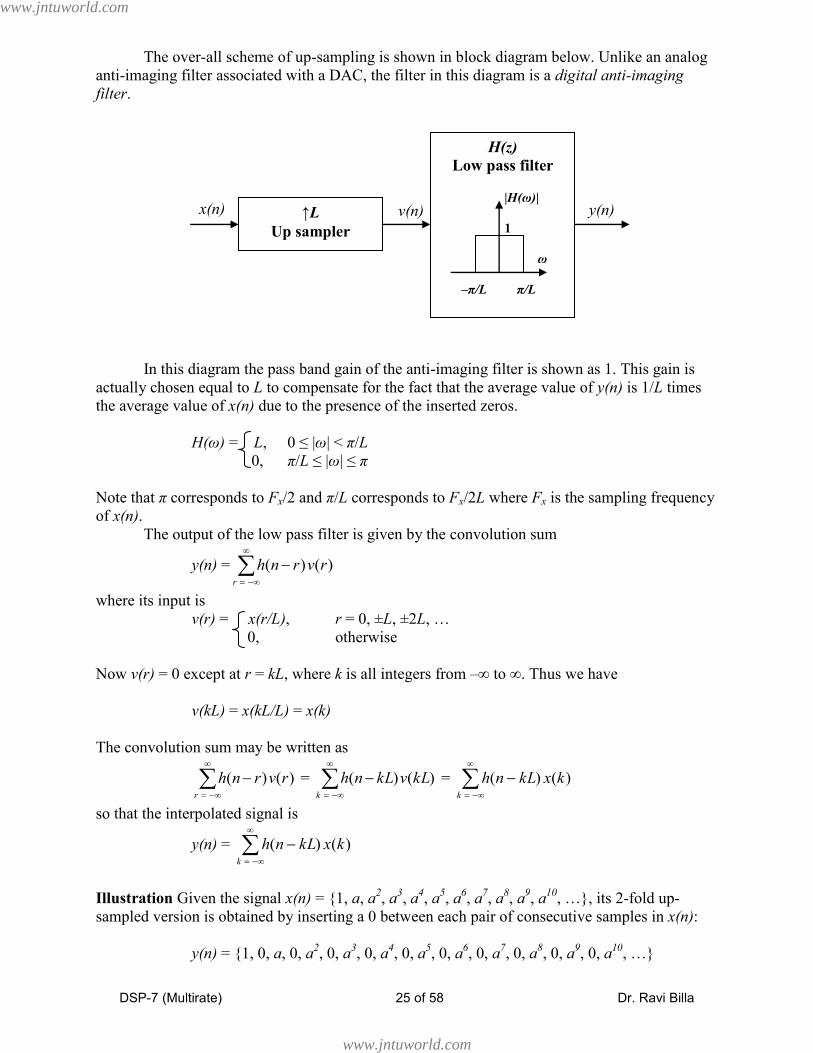
The over-all scheme of up-sampling is shown in block diagram below. Unlike an analog
anti-imaging filter associated with a DAC, the filter in this diagram is a digital anti-imaging
filter.
In this diagram the pass band gain of the anti-imaging filter is shown as 1. This gain is
actually chosen equal to L to compensate for the fact that the average value of y(n) is 1/L times
the average value of x(n) due to the presence of the inserted zeros.
H(ω) = L, 0 ≤ |ω| < π/L
0, π/L ≤ |ω| ≤ π
Note that π corresponds to Fx/2 and π/L corresponds to Fx/2L where Fx is the sampling frequency
of x(n).
The output of the low pass filter is given by the convolution sum
y(n) =
r
rvrnh )()(
where its input is
v(r) = x(r/L), r = 0, ±L, ±2L, …
0, otherwise
Now v(r) = 0 except at r = kL, where k is all integers from –∞ to ∞. Thus we have
v(kL) = x(kL/L) = x(k)
The convolution sum may be written as
r
rvrnh )()( =
k
kLvkLnh )()( =
k
kxkLnh )()(
so that the interpolated signal is
y(n) =
k
kxkLnh )()(
Illustration Given the signal x(n) = {1, a, a2, a
3, a
4, a
5, a
6, a
7, a
8, a
9, a
10, …}, its 2-fold up-
sampled version is obtained by inserting a 0 between each pair of consecutive samples in x(n):
y(n) = {1, 0, a, 0, a2, 0, a
3, 0, a
4, 0, a
5, 0, a
6, 0, a
7, 0, a
8, 0, a
9, 0, a
10, …}
v(n) x(n) y(n) ↑L
Up sampler
H(z)
Low pass filter
|H(ω)|
1
ω
–π/L π/L
www.jntuworld.com
www.jntuworld.com
DSP-7 (Multirate) 26 of 58 Dr. Ravi Billa
Intuitively, even visually, y(n) contains higher (or, more) frequencies than x(n) because of the
inserted zeros. For instance, consider the first two or three samples in each sequence. In the case
of x(n) the changes from 1 to a to a2 are smoother than the fluctuations in y(n) from 1 to 0 to a to
0 to a2; these latter fluctuations are the higher frequencies not originally contained in x(n). It is
these higher frequencies that are represented by the image in the spectrum of y(n) prior to anti-
imaging filtering. The anti-imaging filter removes or smoothes out the higher frequency
fluctuations from the up-sampled version; this smoothing is manifested in the form of the
interpolated zeros being replaced by nonzero values.
7.5 Cascading sampling rate converters
Given a discrete-time signal x(n) we may want to convert its sampling rate by a non integer
factor, in particular, by a rational number. For instance, we may be interested in x(3n/2). This
involves a 2-fold up-sampling and a 3-fold down-sampling for a net down sampling by a factor
of 1.5 (= 3/2). The sequence x(3n/5) involves a 5-fold up-sampling and a 3-fold down-sampling
for a net up-sampling by a factor of 1.67 (= 5/3).
In general, in a cascade of an M-fold down-sampler and an L-fold up-sampler the
positions of the two samplers are inter-changeable with no difference in the input-output
behavior if and only if M and L are co-prime (relatively prime, that is, M and L do not have a
common factor). The sequence x(3n/2) may be generated by cascading the up-sampler and the
down-sampler in either order, that is, down followed by up or vice versa. However, a cascade of
a 6-fold down-sampler (M = 6) followed by a 4-fold up-sampler (L = 4) is not the same as a
cascade of a 4-fold up-sampler followed by a 6-fold down-sampler even though in both cases
M/L = 6/4. This is because M and L have a common factor, that is, the rational number M/L is not
in its reduced form. The ratio M/L should be reduced to 3/2; then the 3-fold down-sampler and
the 2-fold up-sampler are interchangeable in position.
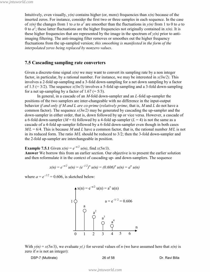
Example 7.5.1 Given x(n) = e–n/2
u(n), find x(5n/3).
Answer We borrow this from an earlier section. Our objective is to present the earlier solution
and then reformulate it in the context of cascading up- and down-samplers. The sequence
x(n) = e–n/2
u(n) = (e–1/2
)n u(n) = (0.606)
n u(n) = a
n u(n)
where a = e–1/2
= 0.606, is sketched below:
With y(n) = x(5n/3), we evaluate y(.) for several values of n (we have assumed here that x(n) is
zero if n is not an integer):
0 1 2 3 4 5 6
x(n) = e–n/2
u(n) = an u(n)
n
1
a2
a3
a4
a
a = e–1/ 2
= 0.606
www.jntuworld.com
www.jntuworld.com

DSP-7 (Multirate) 27 of 58 Dr. Ravi Billa
y(0) = x(5 . 0 / 3) = x(0) = e–0/ 2
= 1
y(1) = x(5 . 1 / 3) = x(5 / 3) = 0
y(2) = x(5 . 2 / 3) = x(10 / 3) = 0
y(3) = x(5 . 3 / 3) = x(5) = e–5/ 2
= a5
…
y(6) = x(5 . 6 / 3) = x(10) = e–10/ 2
= a10
…
The general expression for y(n) can be written as
y(n) = x(5n/3) = e–(5n/3)/2
, n as specified below
= e–5n/ 6
, n = 0, 3, 6, …
0, otherwise
n = 0 1 2 3 4 5 6 7 8 9 10 11 12. . .
y(n) = {1 0 0 a5 0 0 a
10 0 0 a
15 0 0 a
20 . .}
The sequence is sketched below:
We shall recast this problem in terms of cascading the up- and down-samplers. In the
expression y(n) = x(5n/3) there is a 3-fold up-sampling and a 5-fold down-sampling. Since the
numerator 5 is greater than the denominator 3 there is a net down-sampling by a factor of 1.67
(= 5/3). Let us first do a 3-fold up-sampling of x(n) followed by a 5-fold down-sampling of the
resulting sequence. That is, given the sequence x(n)
n = 0 1 2 3 4 5 6 7 8 9 10 . .
x(n) = {1 a a2 a
3 a
4 a
5 a
6 a
7 a
8 a
9 a
10 . .}
0 1 2 3 4 5 6
y(n) = x(5n/3) = e–5n/ 6
, n = 0, 3, 6, …
0, otherwise
n
1
a5
a10
a = e–1/ 2
= 0.606
y(n) = x(5n/3) x(n) yu(n) = x(n/3) ↓5 ↑3
www.jntuworld.com
www.jntuworld.com

DSP-7 (Multirate) 28 of 58 Dr. Ravi Billa
we define yu(n) = x(n/3), and then y(n) = yu(5n) = x(5n/3). The sequences yu(n) and y(n) are given
below.
yu(n) = x(n/3) = e–n/6
u(n/3) = an/3
n = 0, 3, 6, …
0, otherwise
y(n) = yu(5n) = x(5n/3) = e–5n/6
u(5n/3) = a5n/3
n = 0, 3, 6, …
0, otherwise
Alternatively, we may first do a 5-fold down sampling followed by a 3-fold up-sampling:
yd(n) = x(5n) = {1, a5, a
10, a
15, a
20, … }
y(n) = yd(n/3) = x(5n/3) = {1, 0, 0, a5, 0, 0, a
10, 0, 0, a
15, 0, 0, a
20, … }
The net effect is that between the first two terms (1 and a5) of the final output y(.) we
have dropped four original terms and inserted two zeros.
Example 7.5.2 Given x(n) = e–n/2
u(n), find x(3n/5). Here there is a 5-fold up-sampling and a 3-
fold down sampling. Since the denominator is bigger there is a net up-sampling by a factor of
1.67.
x(n) = {1, a, a2, a
3, a
4, a
5, a
6, a
7, a
8, a
9, a
10, …}
Method A Up-sampling followed by down sampling is given below. The 5-fold up-sampled
signal, yu(n), is obtained by inserting 4 zeros shown in bold face between every pair of
consecutive samples in x(n)
yu(n) = x(n/5)
= {1, 0, 0, 0, 0, a, 0, 0, 0, 0, a2, 0, 0, 0, 0, a
3, 0, 0, 0, 0, a
4, 0, 0, 0, 0,
a5, 0, 0, 0, 0, a
6, 0, 0, 0, 0, a
7, 0, 0, 0, 0, a
8, 0, 0, 0, 0, a
9,
0, 0, 0, 0, a10
, …}
The 3-fold down-sampled signal, y1(n), is obtained by keeping every third sample in yu(n) and
discarding the rest (shown underlined)
yu(n) = = {1, 0, 0, 0, 0, a, 0, 0, 0, 0, a2, 0, 0, 0, 0, a
3, 0, 0, 0, 0, a
4, 0, 0, 0, 0,
yu(n) = x(n/3)
n = 0 1 2 3 4 5 6 7 8 9 10 11 12 13 14 15 16 17 . .
yu(n) = {1 0 0 a 0 0 a2 0 0 a
3 0 0 a
4 0 0 a
5 . . . .}
y(n) = yu(5n) = x(5n/3)
n = 0 1 2 3 4 5 6 7 8 9 10 11 12 13 14 15 16 17 . .
y(n) = {1 0 0 a5 0 0 a
10 0 0 a
15 0 0 a
20 0 0 a
25 . . . .}
y(n) = x(5n/3) x(n) yd(n) = x(5n) ↑3 ↓5
www.jntuworld.com
www.jntuworld.com

DSP-7 (Multirate) 29 of 58 Dr. Ravi Billa
a5, 0, 0, 0, 0, a
6, 0, 0, 0, 0, a
7, 0, 0, 0, 0, a
8, 0, 0, 0, 0, a
9,
0, 0, 0, 0, a10
, …}
y1(n) = yu(3n) = x(3n/5)
= {1, 0, 0, 0, 0, a3, 0, 0, 0, 0, a
6, 0, 0, 0, 0, a
9, 0, …}
Method B Down-sampling followed by up sampling is given below. The 3-fold down-sampled
signal, yd(n), is obtained by keeping every third sample in x(n) and discarding the rest (shown
umderlined)
x(n) = {1, a, a2, a
3, a
4, a
5, a
6, a
7, a
8, a
9, a
10, a
11,…}
yd(n) = x(3n) = {1, a3, a
6, a
9, a
12,…}
The 5-fold up-sampled signal, y2(n), is obtained by inserting 4 zeros shown in bold face between
every pair of samples in yd(n)
y2(n) = yd(n/5) = x(3n/5)
y2(n) = {1, 0, 0, 0, 0, a3, 0, 0, 0, 0, a
6, 0, 0, 0, 0, a
9, 0, 0, 0, 0, a
12, …}
= {1, 0, 0, 0, 0, a3, 0, 0, 0, 0, a
6, 0, 0, 0, 0, a
9, 0, 0, 0, 0, a
12, …}
It is seen that y1(n) = y2(n).
Example 7.5.3 Given that x(n) = {1, a, a2, a
3, a
4, a
5, a
6, a
7, a
8, a
9, a
10, …} is the input,
1. Find the output y1(n) of a cascade of a 2-fold up-sampler followed by a 4-fold down
sampler.
2. Find the output y2(n) of a cascade of a 4-fold down sampler followed by a 2-fold up-
sampler.
Solution Note that the down-sampling factor M = 4 and the up-sampling factor L = 2 are not co-
prime since they have a factor in common. The ratio M/L = 4/2, as given, is not in its reduced
form. As a result we do not expect that y1(n) and y2(n) will be equal. Specifically, in the first case
we have
x(n) = {1, a, a2, a
3, a
4, a
5, a
6, a
7, a
8, a
9, a
10, …}
Up-sample by inserting a zero (shown bold face) between consecutive samples of x(n) resulting
in yu(n)
yu(n) = x(n/2) = {1, 0, a, 0, a2, 0, a
3, 0, a
4, 0, a
5, 0, a
6, 0, a
7, 0, a
8, 0, a
9, 0, a
10, …}
Down-sample by keeping every fourth sample of yu(n) and discarding the three samples in
between resulting in y1(n)
y1(n) = yu(4n) = x(4n/2) = {1, a2, a
4, a
6, a
8, a
10, …}
In the second case
x(n) = {1, a, a2, a
3, a
4, a
5, a
6, a
7, a
8, a
9, a
10, …}
yd(n) = x(4n) = {1, a4, a
8, a
12, …}
www.jntuworld.com
www.jntuworld.com

DSP-7 (Multirate) 30 of 58 Dr. Ravi Billa
y2(n) = yd(n/2) = x(4n/2) = {1, 0, a4, 0, a
8, 0, a
12, …}
It is seen that y1(n) ≠ y2(n).
Sampling Rate Conversion by a Rational Factor L/M Here the sampling rate is being
converted by a non-integral factor such as 0.6 or 1.5. That is, given x(n) with a sampling rate of
Fx we want to obtain y(n) with a sampling rate of Fy of, say, 0.6Fx (decimation) or 1.5Fx
(interpolation).
Take, for instance L/M = 3/5. Here the basic approach is to first interpolate (up-sample)
by a factor of L = 3 and then decimate (down-sample) by a factor of M = 5. The net effect of the
cascade of interpolation followed by decimation is to change the sampling rate by a rational
factor L/M, that is,
Fy =
M
LFx =
5
3Fx = 0.6 Fx.
The corresponding signal is given by y(n) = x(5n/3), ignoring the filters involved. (This can also
be done by first down-sampling and then up-sampling).
The block diagram of the scheme where the interpolator precedes the decimator is shown
below.
In general, if L < M we have a rational decimator and if L > M we have a rational
interpolator. In this set-up interpolation is done before decimation in order to work at the higher
sampling rate so as to preserve the original spectral characteristics of x(n). Recall that unless x(n)
was originally over-sampled, decimation in itself or decimation prior to interpolation will modify
the spectrum of x(n) irrecoverably.
The above configuration has an added benefit that the two filters Hu(z) and Hd(z) in series
(which operate at the same sampling rate) can be combined into a single equivalent low pass
filter with a frequency response of H(ω) = Hu(ω)Hd(ω). The simplified configuration is shown
below.
Fx LFx LFx/M
x(n) y(n)
Rational sampling rate conversion
Interpolator
LFx
Hu(z)
↑L
Decimator
LFx
↓M
Hd(z)
LFx/M Fx
x(n) y(n)
Rational sampling rate conversion
v(n) w(n)
LFx
H(z)
↑L
↓M
www.jntuworld.com
www.jntuworld.com

DSP-7 (Multirate) 31 of 58 Dr. Ravi Billa
The bandwidth of the anti-imaging filter Hu(z) is π/L rad., and that of the anti-aliasing
filter Hd(z) is π/M rad., so that the bandwidth of the composite anti-imaging and anti-aliasing
filter H(ω) is
ωc =
ML
,min
and the frequency response is given by
H(ω) = L, 0 ≤ |ω| < ωc
0, ωc ≤ |ω| ≤ π
In the time domain, the output of the up-sampler, v(n), is given by
v(n) = x(n/L), n = 0, ±L, ±2L, …
0, otherwise
and the output of the linear time-invariant filter H(z) is
w(n) =
k
kvknh )()(
Since v(k) = 0 except at k = rL, where r is an integer between –∞ to ∞, we set k = rL. As k goes
from –∞ to ∞, r goes from –∞ to ∞, and v(rL) = x(rL/L) = x(r).
w(n) =
r
rLvrLnh )()( =
r
rxrLnh )()( =
k
kxkLnh )()(
Finally the output of the down sampler is
y(n) = w(Mn) =
k
kxkLMnh )()(
In summary, sampling rate conversion by the factor L/M can be achieved by first
increasing the sampling rate by L, accomplished by inserting L–1 zeros between successive
samples of the input x(n), followed by linear filtering of the resulting sequence to eliminate
unwanted images of X(ω) and, finally, by down-sampling the filtered signal by the factor M to
get the output y(n). The sampling rates are related by Fy = (L/M)Fx. If Fy > Fx, that is, L > M, the
low pass filter acts as an anti-imaging post-filter to the up-sampler. If Fy < Fx, that is, L < M, the
low pass filter acts as an anti-aliasing pre-filter to the down-sampler.
www.jntuworld.com
www.jntuworld.com

DSP-7 (Multirate) 32 of 58 Dr. Ravi Billa
Example 7.5.4 The signal x(t) = cos 2π2t + 0.8 sin 2π4t is sampled at 40 Hz to generate x(n).
a) Give an expression for x(n)
b) Design a sampling rate converter to change the sampling frequency of x(n) by a
factor of 2.5. Give an expression for y(n).
c) Design a sampling rate converter to change the sampling frequency of x(n) by a
factor of 0.4. Give an expression for y(n).
Solution
a) x(n) = cos 2π2nT + 0.8 sin 2π4nT = cos πn/10 + 0.8 sin πn/5
b) The rate conversion factor is L/M = 2.5 = 5/2. We do this by first up-sampling by a factor of 5,
then down-sampling by a factor of 2. Roughly speaking, y(n) = x(2n/5).
The up-sampling requires an anti-imaging LP filter of bandwidth of π/L = π/5 rad., and a
gain of 5. The down-sampling requires an anti-aliasing LP filter of band width π/M = π/2 rad.
When the up-sampler precedes the down-sampler we have the following configuration where the
filter has the smaller of the two band widths, that is, π/5 rad. The gain is 5 and is always
determined by the up-sampler.
Write equations for v(n), w(n), and y(n) based on the above diagram and assuming H(z) is
an FIR filter of N coefficients.
c) The rate conversion factor is L/M = 0.4 = 2/5. We do this by first up-sampling by a factor of 2,
then down-sampling by a factor of 5. Roughly speaking, y(n) = x(5n/2). Band width of filter =
π/5 rad., and gain = 2, once again determined by the up-sampler.
Write equations for v(n), w(n), and y(n) based on the above diagram and assuming H(z) is
an FIR filter N coefficients.
Multistage conversion The composite anti-imaging and anti-aliasing LP filter band width is π/L
or π/M whichever is smaller. That is, the filter band width is determined by the larger number of
L and M. However, if either L or M is a very large number the filter bandwidth is very narrow.
5Fx/2 Fx
x(n) y(n)
Rational sampling rate conversion
v(n) w(n)
5Fx
H(z)
↑5
↓2
2Fx/5 Fx
x(n) y(n)
Rational sampling rate conversion
v(n) w(n)
2Fx
H(z)
↑2
↓5
www.jntuworld.com
www.jntuworld.com

DSP-7 (Multirate) 33 of 58 Dr. Ravi Billa
Narrowband FIR (linear phase) filters can require a very large number of coefficients (see Unit
VI, FIR Filters, Example 6). This can pose problems in
1. Increased storage space for coefficients,
2. Long computation time, and
3. Detrimental finite word length effects
The latter drawback is minimized by using a multistage sampling rate converter where the
conversion ratio L/M is factored into the product of several ratios each of which has its own
smaller L and M values. If, for instance, the ratio L/M is split into the product of two ratios
M
L=
1
1
M
L
2
2
M
L
where the L’s and M’s on the right hand side are smaller, we may implement the rate conversion
in two stages as shown below
Example 7.5.5 [Rational sampling rate converter][CD, DAT] Digital audio tape (DAT) used
in sound recording studios has a sampling rate of 48 kHz, while a compact disc (CD) is recorded
at a sampling rate of 44.1 kHz. Design a sampling rate converter that will convert the DAT
signal x(n) to a signal y(n) for CD recording.
Over-sampling analog-to-digital converter (ADC) [Ref. SKMitra, Sec 4.8.4] A practical
difficulty with analog to digital conversion is the need for a low pass analog anti-aliasing
prefilter to band limit the signal to less than half of the sampling rate. High-order analog filters
are expensive, and they are also difficult to keep in calibration. The combination of over-
sampling followed by down-sampling can be used to transfer some of the anti-aliasing burden
from the analog into the digital domain, and thereby use a simpler low order analog filter.
As an example, a typical compact disk encoding system may employ an over-sampling
sigma-delta A/D converter which over-samples at 3175.2 kHz which is then brought down to the
CD sampling rate of 44.1 kHz. This amounts to over-sampling by a factor of 72 (= 3175.2/44.1).
Suppose the range of frequencies of interest in the signal x(t) is 0 ≤ |F| ≤ FM. Normally
we would band-limit x(t) to the maximum frequency FM with a sharp cut-off analog low pass
filter and sample it at a rate of Fs = 2FM at least (strictly, Fs ≥ 2FM). Suppose that we instead
over-sample x(t) by an integer factor M, at Fs = M (2FM). This significantly reduces the
requirements for the anti-aliasing filter which may be specified more leniently as
Ha(s) = 1, 0 |F| FM
0, MFM |F| < ∞
Stage 1
↑L1 H1(z) ↓M1
Stage 2
↑L2 H2(z) ↓M2
www.jntuworld.com
www.jntuworld.com

DSP-7 (Multirate) 34 of 58 Dr. Ravi Billa
Though this is still an ideal low pass filter in the pass band and stop band, its transition band
width is no longer zero and it may be approximated with an inexpensive first- or second-order
Butterworth filter as shown below.
We are paying the price of a higher sampling rate for the benefit of a cheaper analog
anti-aliasing filter. The result is a discrete-time signal that is sampled at a much higher rate than
2FM. Following the sampling operation, we can reduce this sampling rate to the minimum value
using a decimator. The resulting structure of the over-sampling ADC is shown in the block
diagram below. There are two anti-aliasing filters, a low-order analog filter Ha(s) with cut-off
frequency FM rad/sec., and a high-order digital filter Hd(z), with a cut-off frequency (π/M)
rad/sample.
A second benefit of using the over-sampling ADC is the reduction in quantization noise.
If q is the quantization step size (precision), then the quantization noise in x(n) is 2
x = 122q ,
and the noise appearing in the output y(n) in the above scheme is 2
y = Mx
2 = Mq 122 , a
reduction by a factor of M.
0 F, Hz
|Ha(F)| with over-sampling
1
FM MFM
Pass Transition band
(Unspecified) Stop Band
0 F, Hz
|Ha(F)| without over-sampling
1
FM MFM
Pass Stop Band
2FM
samples/sec
M(2FM)
samples/sec
Over-sampling AD converter
x(t) y(n) x(n) Ha(s) ADC Hd(z) ↓M
www.jntuworld.com
www.jntuworld.com
DSP-7 (Multirate) 35 of 58 Dr. Ravi Billa
7.6 Identities
A sampling rate converter (the ↓M or ↑L operation) is a linear time-varying system. On the other
hand, the filters Hd(z) and Hu(z) are linear time-invariant systems. In general, the order of a
sampling rate converter and a linear time-invariant system cannot be interchanged. We derive
below several identities, two of which are known as noble identities (viz., identities 3 and 6, all
the others being special cases), which help to swap the position of a filter with that of a down-
sampler or up-sampler by properly modifying the filter.
Recall that the input-output description of a down-sampler is
y(n) = x(Mn) ↔ Y(z) = M
1
1
0
/1/2M
k
MMkj zeX ↔ Y(ejω
) = M
1
1
0
/)2(M
k
MkjeX
and the same for an up-sampler is
y(n) = x(n/L), n = 0, ±L, ±2L, … ↔ Y(z) = X(zL) ↔ Y(e
jω) = X(e
jωL)
0, otherwise
which we use in the following development.
Example 7.6.1 Show that the following systems are equivalent.
In the structure on the left the process of generating y(.) consists of multiplying every input
sample x(.) by a and then, in the down-sampling process, dropping (M–1) of these products for
every Mth
one we keep. The structure on the right is more efficient computationally: the (M–1)
samples are dropped first and every Mth
is multiplied by a, that is, only the samples that are
retained are multiplied. The number of multiplications is reduced by M
M )1(100 %.
Example 7.6.2 Show that the following systems are equivalent.
In the structure on the left the process of generating y(.) consists of first up-sampling, that is,
inserting zeros between consecutive points of x(n) and then multiplying by a. In the process the
(L–1) zeros are also multiplied. The structure on the right is more efficient computationally: the
sequence x(n) is first multiplied and then the zeros inserted. The number of multiplications is
reduced by L
L )1(100 %.
v(n) y(n) x(n) a
↓M w(n) y(n) x(n) a
↓M
v(n) y(n) x(n) a
↑L w(n) y(n) x(n) a
↑L
www.jntuworld.com
www.jntuworld.com

DSP-7 (Multirate) 36 of 58 Dr. Ravi Billa
Identity #1 If we use the notation ↓M{.} to mean the down-sampling of the signal in braces, then
we have
↓M{a x1(n) + b x2(n)} = ↓M{a x1(n)} + ↓M{b x2(n)} → (1)
= a ↓M{x1(n)} + b ↓M{x2(n)} → (2)
In words, the result of down-sampling the weighted sum of signals equals the weighted sum of
the down-sampled signals. In other words, the two block diagrams below are equivalent.
In the diagram on the left the weighted sum of two inputs is down-sampled:
w(n) = a x1(n) + b x2(n) ↔ W(ejω
) = a X1(ejω
) + b X2(ejω
)
The output and its spectrum are then given by
y(n) = w(Mn)
Y(ejω
) = M
1
1
0
/)2(M
k
MkjeW
= M
a
1
0
/)2(
1
M
k
MkjeX + M
b
1
0
/)2(
2
M
k
MkjeX → (A)
In the diagram on the right the weighted inputs are down-sampled and added to form the
output.
y1(n) = a x1(Mn) ↔ Y1(ejω
) = M
a
1
0
/)2(
1
M
k
MkjeX
y2(n) = b x2(Mn) ↔ Y2(ejω
) = M
b
1
0
/)2(
2
M
k
MkjeX
The output and its spectrum are given by
y(n) = y1(n) + y2(n)
Y(ejω
) = Y1(ejω
) + Y2(ejω
) = M
a
1
0
/)2(
1
M
k
MkjeX +
M
b
1
0
/)2(
2
M
k
MkjeX → (B)
Equations (A) and (B) are identical. QED.
Eventually, by virtue of Example 6.1, the down-samplers are moved to the upstream side
of the multipliers which would correspond to Eq. (2).
Identity #2 A delay of M sample periods before an M-fold down-sampler is the same as a delay
of one sample period after the down-sampler.
w(n)
x1(n)
x2(n)
a
b
y(n) ↓M
y1(n)
y2(n)
x1(n)
x2(n)
a
b
y(n)
↓M
↓M
www.jntuworld.com
www.jntuworld.com

DSP-7 (Multirate) 37 of 58 Dr. Ravi Billa
In the first case (diagram on the left) we have
y1(n) = x(n–M) ↔ Y1(z) = z–M
X(z) → (1)
and
y(n) = y1(Mn) ↔ Y(z) = M
1
1
0
/1/2
1
M
k
MMkj zeY → (2)
Note from (1) that
MMkj zeY /1/2
1
= MMkj zezzY /1/21
= MMkj zez
M zXz/1/2
)(
= MMkjMMMkj zeXze /1/2/1/2
Substituting this in (2) we have
Y(z) = M
1
1
0
/1/2/1/2M
k
MMkjMMMkj zeXze
= M
1
1
0
/1/2//2M
k
MMkjMMMMkj zeXze = M
1
1
0
/1/211M
k
MMkj zeXz
= z–1
M
1
1
0
/1/2M
k
MMkj zeX → (A)
In the second case (diagram on the right) we have
y2(n) = x(nM) ↔ Y2(z) = M
1
1
0
/1/2M
k
MMk zeX → (3)
y(n) = y2(n–1) ↔ Y(z) = z–1
Y2(z) → (4)
Substituting from (3) into (4) we have
Y(z) = z–1
Y2(z) = z–1
M
1
1
0
/1/2M
k
MMk zeX → (B)
Equations (A) and (B) are identical. QED.
Identity #3 (Noble identity) An M-fold down-sampler followed by a linear time invariant filter
H(z) is equivalent to a linear time invariant filter H(zM
) followed by an M-fold down-sampler.
Note that the second identity is a special case of this identity with H(z) = z–1
and H(zM
) = z–M
.
For the system consisting of the filter followed by the down-sampler we have
Y1(z) = H(zM
) X(z)
y1(n) x(n) y(n) z–M
↓M y2(n) x(n) y(n)
↓M z–1
y1(n) x(n) y(n) H(z
M) ↓M
y2(n) x(n) y(n) ↓M H(z)
www.jntuworld.com
www.jntuworld.com

DSP-7 (Multirate) 38 of 58 Dr. Ravi Billa
Y(z) = M
1
1
0
/1/2
1
M
k
MMkj zeY
Note that
MMkj zeY /1/2
1
= MMkj zezzY /1/21
= MMkj zez
M zXzH/1/2
= MMkjMMMkj zeXzeH /1/2/1/2
= MMkjMMMMkj zeXzeH /1/2//2
= MMkj zeXzH /1/21 = H(z) MMkj zeX /1/2
Thus
Y(z) = M
1
1
0
/1/2)(M
k
MMkj zeXzH
= H(z) M
1
1
0
/1/2M
k
MMkj zeX → (A)
For the system consisting of the down sampler followed by the filter we have
y2(n) = x(nM)
Y2(z) = M
1
1
0
/1/2M
k
MMk zeX
Y(z) = H(z) Y2(z) = H(z) M
1
1
0
/1/2M
k
MMk zeX → (B)
Equations (A) and (B) are identical. Thus the two systems are equivalent.
www.jntuworld.com
www.jntuworld.com

DSP-7 (Multirate) 39 of 58 Dr. Ravi Billa
Identity #4 (This identity contains no summing junction as does identity #1.) Eventually, by
virtue of Example 6.2, the up-samplers are moved to the downstream side of the multipliers.
Identity #5 A delay of one sample period before an L-fold up-sampler is the same as a delay of L
sample periods after the up-sampler.
For the system consisting of the up-sampler preceded by z–1
we have
Y1(z) = z–1
X(z)
Y(z) = Y1(zL) = z
–L X(z
L) → (A)
For the system consisting of the up-sampler followed by z–L
we have
Y2(z) = X(zL)
Y(z) = z–L
Y2(z) = z–L
X(zL) → (B)
Since equations (A) and (B) are identical the two systems are equivalent.
Identity #6 (Noble identity) An L-fold up-sampler preceded by a linear time invariant filter H(z)
is equivalent to a linear time invariant filter H(zL) preceded by an L-fold up-sampler. Note that
the fifth identity is a special case of this identity with H(z) = z–1
and H(zL) = z
–L.
For the system consisting of the filter followed by the up-sampler we have
Y1(z) = H(z) X(z)
Y(z) = Y1(zL) = H(z
L) X(z
L) → (A)
y1(n) x(n) y(n) H(z) ↓L
y2(n) x(n) y(n) ↓L H(z
L)
y1(n) x(n) y(n) z–1
↓L
y2(n) x(n) y(n) ↓L z
–L
y1(n)
y2(n)
x(n)
a
b
v(n) ↑L
v(n)
v(n)
y1(n)
y2(n)
x(n)
a
b ↑L
↑L
www.jntuworld.com
www.jntuworld.com

DSP-7 (Multirate) 40 of 58 Dr. Ravi Billa
For the system consisting of the up-sampler followed by the filter we have
Y2(z) = X(zL)
Y(z) = H(zL) Y2(z) = H(z
L) X(z
L) → (B)
Since equations (A) and (B) are identical the two systems are equivalent.
www.jntuworld.com
www.jntuworld.com

DSP-7 (Multirate) 41 of 58 Dr. Ravi Billa
7.7 FIR implementation of sampling rate conversion
The anti-aliasing filter in a decimator and the anti-imaging filter in an interpolator may each be
either an FIR or an IIR filter, the former being preferred since it offers linear phase. We give here
the FIR implementation.
Implementation of Decimator The process of decimation consists of an anti-aliasing (low pass)
filter followed by a down-sampler. We repeat below the block diagram developed earlier.
Taking the filter H(z) to be an FIR filter, the decimator is implemented as shown below,
using a direct form structure for H(z). Note that the coefficients {bi, i = 0 to (N–1)}, used in
earlier formulations, are the same as {h(i), i = 0 to (N–1)} used in this diagram. Further, the FIR
filter here is implemented with N coefficients rather than (N+1) coefficients.
h(N–2)
h(N–1)
h(1)
h(2)
v(n) x(n) h(0) y(n)
z–1
z–1
z–1
↓M
x(n) v(n) y(n) ↓M
Down sampler
H(z)
Low pass filter
|H(ω)|
1
ω
–π/M π/M
www.jntuworld.com
www.jntuworld.com
DSP-7 (Multirate) 42 of 58 Dr. Ravi Billa
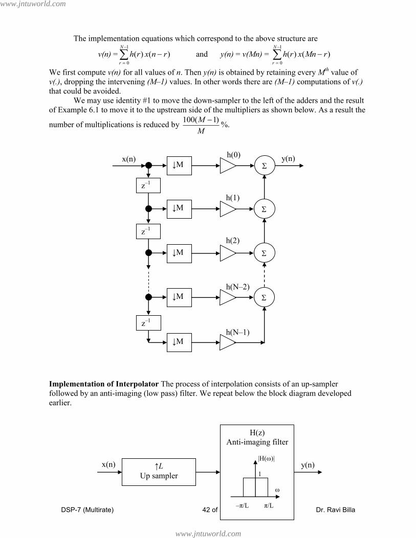
The implementation equations which correspond to the above structure are
v(n) =
1
0
)()(N
r
rnxrh and y(n) = v(Mn) =
1
0
)()(N
r
rMnxrh
We first compute v(n) for all values of n. Then y(n) is obtained by retaining every Mth
value of
v(.), dropping the intervening (M–1) values. In other words there are (M–1) computations of v(.)
that could be avoided.
We may use identity #1 to move the down-sampler to the left of the adders and the result
of Example 6.1 to move it to the upstream side of the multipliers as shown below. As a result the
number of multiplications is reduced by M
M )1(100 %.
Implementation of Interpolator The process of interpolation consists of an up-sampler
followed by an anti-imaging (low pass) filter. We repeat below the block diagram developed
earlier.
h(N–2)
h(N–1)
h(1)
h(2)
x(n) h(0) y(n)
z–1
z–1
z–1
↓M
↓M
↓M
↓M
↓M
x(n) y(n) ↑L
Up sampler
H(z)
Anti-imaging filter
|H(ω)|
1
ω
–π/L π/L
www.jntuworld.com
www.jntuworld.com

DSP-7 (Multirate) 43 of 58 Dr. Ravi Billa
Taking the filter H(z) to be an FIR filter, the interpolator is implemented as shown below,
using a direct form structure for H(z). Note that the coefficients {bi, i = 0 to (N–1)}, used in
earlier formulations, are the same as {h(i), i = 0 to (N–1)} used in this diagram. Further, the FIR
filter here is implemented with N coefficients rather than (N+1) coefficients.
We shall find it more convenient to use the transposed form of the FIR filter rather than
the structure actually shown here, so here follows a digression on the transposed structure.
h(N–2)
h(N–1)
h(1)
h(2)
x(n) h(0) y(n)
↑L
z–1
z–1
z–1
www.jntuworld.com
www.jntuworld.com

DSP-7 (Multirate) 44 of 58 Dr. Ravi Billa
Start of Digression Transposed Structure According to the transposition theorem the transposed form of a filter
has the same transfer function as the filter. The transposed form of a given filter structure is
found as follows:
1. Construct the signal flow graph of the filter.
2. Reverse the direction of arrow on every branch.
3. Interchange the inputs and outputs.
4. Reverse the roles of all nodes: an adder becomes a pick-off point and a pick-off
point becomes an adder.
If we apply this procedure to the FIR structure in the above interpolator the result is the transpose
shown below. The intermediate steps are omitted.
Start of Aside
As an aside note that the FIR structure is simple enough that the following algebraic
manipulation can be used to proceed from the original FIR structure to the transpose structure.
Let the system function be
h(N–2)
h(N–1)
h(1)
h(2)
u(n) h(0) v(n)
z–1
z–1
z–1
Original
h(N–2)
h(N–1)
h(1)
h(2)
u(n) h(0) v(n)
z–1
z–1
z–1
z–1
Transpose
www.jntuworld.com
www.jntuworld.com

DSP-7 (Multirate) 45 of 58 Dr. Ravi Billa
)(
)(
zU
zV = )( zH = )0(h + 1)1( zh + 2)2( zh + 3)3( zh + 4)4( zh + … + )1()1( NzNh
This may be rearranged as
)( zV = )()( zUzH
= )()0( zUh + )()1( 1 zUzh + )()2( 2 zUzh + )()3( 3 zUzh + )()4( 4 zUzh + …
+ )()1( )1( zUzNh N
= )()0( zUh + 1z ( )()1( zUh + 1z ( )()2( zUh + 1z ( )()3( zUh + …
… + 1z ( )()2( zUNh + 1z )()1( zUNh ))))
This last equation, proceeding from right to left, performs the following in the time domain:
Multiply )(nu by )1( Nh , giving )()1( nuNh
Delay by 1 unit, giving )1()1( nuNh
Add to )()2( nuNh , giving )1()1()()2( nuNhnuNh
Delay by 1 unit, giving )2()1()1()2( nuNhnuNh
Add to )()3( nuNh , giving )2()1()1()2()()3( nuNhnuNhnuNh
Delay by 1 unit, giving )3()1()2()2()1()3( nuNhnuNhnuNh
…
Add to )()0( nuh
all of which yields the implementation of the difference equation
)(nv = )()0( nuh + )1()1( nuh + )2()2( nuh + …
…+ )2()2( NnuNh + )1()1( NnuNh
Further, the equation
)( zV = )()0( zUh + 1z ( )()1( zUh + 1z ( )()2( zUh + 1z ( )()3( zUh + …
… + 1z ( )()2( zUNh + 1z )()1( zUNh ))))
also suggests the transpose structure previously developed according to the rules.
End of Aside
End of Digression
www.jntuworld.com
www.jntuworld.com

DSP-7 (Multirate) 46 of 58 Dr. Ravi Billa
Resumption of Implementation of Interpolator Using the transposed form of the FIR filter the
structure of the interpolator appears as below:
“v(n)” “u(n)”
h(N–2)
h(N–1)
h(1)
h(2)
h(0) y(n)
Transpose
x(n)
z–1
z–1
z–1
z–1
↑L
www.jntuworld.com
www.jntuworld.com

DSP-7 (Multirate) 47 of 58 Dr. Ravi Billa
We may use identity #4 and the result of Example 6.2 to move the up-sampler to the right
of the multipliers as shown below. As a result the number of multiplications is reduced by
L
L )1(100 %.
h(N–2)
h(N–1)
h(1)
h(2)
h(0) y(n) x(n)
z–1
↑L
z–1
↑L
↑L
z–1
↑L
z–1
↑L
www.jntuworld.com
www.jntuworld.com

DSP-7 (Multirate) 48 of 58 Dr. Ravi Billa
7.8 Polyphase structures
The polyphase structure for FIR Filters was developed for the efficient implementation of
sampling rate converters; however, it can be used in other applications. Further, the polyphase
structure can be developed for any filter, FIR or IIR. We give below an introduction.
Polyphase Structure for FIR Filters The impulse response of the FIR filter h(n) is of finite
length, N. The system function with N coefficients is
H(z) =
1
0
)(N
n
nznh = )0(h + 1)1( zh + 2)2( zh + 3)3( zh + 4)4( zh + … + )1()1( NzNh
We shall use another parameter M: we shall divide the number of coefficients into M groups (or
branches or phases), modulo M. In other words the N terms in H(z) are arranged into M branches
with each branch containing at most 1/1 MNInt terms.
Type 1 polyphase decomposition For illustration, let N = 11 and M =2 so that one group
contains 6 coefficients and the other 5 as developed below:
H(z) =
10
0
)(n
nznh = )0(h + 1)1( zh + 2)2( zh + 3)3( zh + 4)4( zh + … + 10)10( zh
= )0(h + 2)2( zh + 4)4( zh + 6)6( zh + 8)8( zh + 10)10( zh ← 1st group
+ 1)1( zh + 3)3( zh + 5)5( zh + 7)7( zh + 9)9( zh ← 2nd
group
= )0(h + 2)2( zh + 4)4( zh + 6)6( zh + 8)8( zh + 10)10( zh
+ 1z { )1(h + 2)3( zh + 4)5( zh + 6)7( zh + 8)9( zh }
Define
MNInt /1 = integer part of the argument
P0(z) = )0(h + 1)2( zh + 2)4( zh + 3)6( zh + 4)8( zh + 5)10( zh =
2/111
0
)02(Int
n
nznh
(More generally, P0(z) =
MNInt
n
nzMnh/1
0
)0( )
P1(z) = )1(h + 1)3( zh + 2)5( zh + 3)7( zh + 4)9( zh =
2/111
0
)12(Int
n
nznh (h(11) = 0)
(More generally, P1(z) =
MNInt
n
nzMnh/1
0
)1( )
In this specific case we have
)(
)(
zX
zY = H(z) = )( 2
0 zP + 1z )( 2
1 zP =
1
0
2 )(n
m
m zPz
www.jntuworld.com
www.jntuworld.com

DSP-7 (Multirate) 49 of 58 Dr. Ravi Billa
This decomposition of H(z) is known as type 1 polyphase decomposition. The
corresponding structure is shown below. The functions )( 2
0 zP and )( 2
1 zP can each be
implemented as a direct form.
By observing the expressions for P0(z) and P1(z) we can further generalize the functions
Pm(z) for any m as
Pm(z) =
MNInt
n
nzmMnh/1
0
)( ), m = 0 to (M–1)
Further, the system function becomes
)(
)(
zX
zY = H(z) = )(0
MzP + 1z )(1
MzP + … + )1( Mz )(1
M
M zP =
1
0
)(M
m
M
m
m zPz
Example 7.8.1 As another example, let N = 11 and M =3.
H(z) =
10
0
)(n
nznh = )0(h + 1)1( zh + 2)2( zh + 3)3( zh + 4)4( zh + … + 10)10( zh
= )0(h + 3)3( zh + 6)6( zh + 9)9( zh – 1st group
+ 1)1( zh + 4)4( zh + 7)7( zh + 10)10( zh – 2nd
group
+ 2)2( zh + 5)5( zh + 8)8( zh – 3rd
group
H(z) = )0(h + 3)3( zh + 6)6( zh + 9)9( zh
+ 1z { )1(h + 3)4( zh + 6)7( zh + 9)10( zh }
+ 2z { )2(h + 3)5( zh + 6)8( zh }
Define
MNInt /1 = integer part of the argument
P0(z) = )0(h + 1)3( zh + 2)6( zh + 3)9( zh =
3/111
0
)03(Int
n
nznh
(More generally, P0(z) =
MNInt
n
nzMnh/1
0
)0( )
P1(z) = )1(h + 1)4( zh + 2)7( zh + 3)10( zh =
3/111
0
)13(Int
n
nznh
(More generally, P1(z) =
MNInt
n
nzMnh/1
0
)1( )
x(n) y(n)
z–1
P1(z2)
P0(z2)
www.jntuworld.com
www.jntuworld.com

DSP-7 (Multirate) 50 of 58 Dr. Ravi Billa
P2(z) = )2(h + 1)5( zh + 2)8( zh =
3/111
0
)13(Int
n
nznh (h(11) = 0)
(More generally, P2(z) =
MNInt
n
nzMnh/1
0
)1( )
In this specific case we have
)(
)(
zX
zY = H(z) = )( 3
0 zP + 1z )( 3
1 zP + 2z )( 3
2 zP =
2
0
3 )(m
m
m zPz
x(n) y(n)
z–1
P2(z3)
P0(z3)
z–1
P1(z3)
www.jntuworld.com
www.jntuworld.com

DSP-7 (Multirate) 51 of 58 Dr. Ravi Billa
Generalization As mentioned earlier, in the general case for an arbitrary M (≤ N) we have
Pm(z) =
MNInt
n
nzmMnh/1
0
)( , m = 0 to (M–1)
and
)(
)(
zX
zY = H(z) = )(0
MzP + 1z )(1
MzP + … + )1( Mz )(1
M
M zP =
1
0
)(M
m
M
m
m zPz
This overall operation is known as polyphase filtering.
(M–1)th
Delay
x(n) y(n)
z–1
PM–1(zM
)
z–1
PM–2(zM
)
z–1
Pm(zM
)
P0(zM
)
z–1
P1(zM
)
z–1
P2(zM
)
www.jntuworld.com
www.jntuworld.com

DSP-7 (Multirate) 52 of 58 Dr. Ravi Billa
Type 2 polyphase decomposition Given
)(
)(
zX
zY = H(z) = )(0
MzP + 1z )(1
MzP + … + )1( Mz )(1
M
M zP =
1
0
)(M
m
M
m
m zPz
set m = M–1–k: as m goes from 0 to M–1, k goes from M–1 to 0. Thus
H(z) =
0
1
1
)1( )(Mk
M
kM
kM zPz
Let
)( M
k zQ = )(1
)1( M
kM
kM zPz
This gives us the type 2 polyphase decomposition
H(z) =
0
1
)(Mk
M
k zQ =
1
0
)(M
k
M
k zQ = )(0
MzQ + )(1
MzQ + … + )(1
M
M zQ
Type 3 polyphase decomposition Given
)(
)(
zX
zY = H(z) = )(0
MzP + 1z )(1
MzP + … + )1( Mz )(1
M
M zP =
1
0
)(M
m
M
m
m zPz
set m = –k: as m goes from 0 to M–1, k goes from 0 to –(M–1) to 0. Thus
H(z) =
)1(
0
)(M
k
M
k
k zPz
Let
)( M
k zR = )( M
k
k zPz
www.jntuworld.com
www.jntuworld.com

DSP-7 (Multirate) 53 of 58 Dr. Ravi Billa
Example 7.8.2 For the system
H(z) =
6
0
)(n
nznh = )0(h + 1)1( zh + 2)2( zh + 3)3( zh + 4)4( zh + 5)5( zh + 6)6( zh
= { 0h + 2
2
zh + 4
4
zh + 6
6
zh } + { 1
1
zh + 3
3
zh + 5
5
zh }
= { 0h + 2
2
zh + 4
4
zh + 6
6
zh } + 1z { 1h + 2
3
zh + 4
5
zh }
P0(z) = 0h + 1
2
zh + 2
4
zh + 3
6
zh
P1(z) = 1h + 1
3
zh + 2
5
zh
The structure is shown below (left). As mentioned earlier )( 2
0 zP and )( 2
1 zP can each be
implemented as a direct form.
The structure shown on the right is obtained by moving the delay element 1z to the right of
)( 2
1 zP these two being in series in the second phase. In this latter case the two systems )( 2
0 zP
and )( 2
1 zP can share the same delay elements (that is, storage locations) even though each has its
own set of coefficients, thus resulting in a canonical polyphase realization, shown below.
x(n) y(n)
z–1
P1(z2)
P0(z2)
Canonical polyphase realization
x(n) y(n)
z–1
P1(z2)
P0(z2)
Polyphase realization
)( 2
0 zP
)( 2
1 zP
h0 h2 h4 h6
y(n) x(n)
h1 h3 h5
z–1
z–2
z–2
z–2
www.jntuworld.com
www.jntuworld.com

DSP-7 (Multirate) 54 of 58 Dr. Ravi Billa
Polyphase Structure for IIR Filters The anti-aliasing filter in a decimator and the anti-imaging
filter in an interpolator may each be either an FIR or an IIR filter. The polyphase structure can be
developed for any filter, FIR or IIR, and any finite value of M. We now proceed to the case
where h(n) is an infinitely long sequence:
H(z) =
n
nznh )( = …+ MzMh )( +… 2)2( zh + 1)1( zh
+ )0(h + 1)1( zh + 2)2( zh +…+ )1()1( MzMh
+ MzMh )( + )1()1( MzMh …
Once again we arrange the terms into M groups or branches in a modulo-M fashion. Each branch
contains infinitely many terms. The terms are arranged in tabular form below:
H(z) =
n
nznh )(
1st branch→ … + MzMh )( + )0(h + MzMh )( …
2nd
branch→ … + 1)1( MzMh + 1)1( zh + )1()1( MzMh …
… … + 2)2( zh + )2()2( MzMh …
… … … … …
ith
branch→ … )1()1( iMziMh )1()1( izih )1()1( iMziMh …
… … … … …
… + 2)2( zh + )2()2( MzMh + )22()22( MzMh …
Mth
branch→ … + 1)1( zh + )1()1( MzMh + )12()12( MzMh …
H(z) = […+ MzMh )( + )0(h + MzMh )( + MzMh 2)2( +…] 1st row
+ […+ 1)1( MzMh + 1)1( zh + )1()1( MzMh +…] 2nd
row
+ […] + …
+ […+ )1()1( iMziMh + )1()1( izih + )1()1( iMziMh
+ )12()12( iMziMh +…]
…
+ […+ 2)2( zh + )2()2( MzMh + )22()22( MzMh +…]
+ […+ 1)1( zh + )1()1( MzMh + )12()12( MzMh +…] Mth
row
We factor out 0z from the first row (branch), 1z from the 2nd
row, and, in general, )1( iz from the
ith
row to get
H(z) = […+ MzMh )( + )0(h + MzMh )( + MzMh 2)2( +…] 1st row
+ 1z […+ MzMh )1( + )1(h + MzMh )1( +…] 2nd
row
+ 2z […] + …
+ )1( iz […+ MziMh )1( + )1( ih + MziMh )1( + MziMh 2)12( +…]
…
+ )2( Mz […+ Mzh )2( + )2( Mh + MzMh )22( +…]
+ )1( Mz […+ Mzh )1( + )1( Mh + MzMh )12( +…]
Define
www.jntuworld.com
www.jntuworld.com
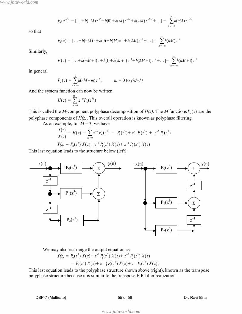
DSP-7 (Multirate) 55 of 58 Dr. Ravi Billa
)(0
MzP = […+ MzMh )( + )0(h + MzMh )( + MzMh 2)2( +…] =
n
nMznMh )(
so that
)(0 zP = […+ zMh )( + )0(h + 1)( zMh + 2)2( zMh +…] =
n
nznMh )(
Similarly,
)(1 zP = […+ zMh )1( + )1(h + 1)1( zMh + 2)12( zMh +…]=
n
nznMh )1(
In general
)( zPm =
n
nzmnMh )( , m = 0 to (M–1)
And the system function can now be written
)( zH =
1
0
)(M
m
M
m
m zPz
This is called the M-component polyphase decomposition of H(z). The M functions )( zPm are the
polyphase components of H(z). This overall operation is known as polyphase filtering.
As an example, for M = 3, we have
)(
)(
zX
zY = )( zH =
2
0
3 )(m
m
m zPz = )( 3
0 zP + 1z )( 3
1 zP + 2z )( 3
2 zP
Y(z) = )( 3
0 zP )( zX + 1z )( 3
1 zP )( zX + 2z )( 3
2 zP )( zX
This last equation leads to the structure below (left):
We may also rearrange the output equation as
Y(z) = )( 3
0 zP )( zX + 1z )( 3
1 zP )( zX + 2z )( 3
2 zP )( zX
= )( 3
0 zP )( zX + 1z { )( 3
1 zP )( zX + 1z )( 3
2 zP )( zX }
This last equation leads to the polyphase structure shown above (right), known as the transpose
polyphase structure because it is similar to the transpose FIR filter realization.
x(n) y(n)
z–1
P2(z3)
P0(z3)
z–1
P1(z3)
x(n) y(n) P0(z
3)
z–1
z–1
P2(z3)
P1(z3)
www.jntuworld.com
www.jntuworld.com

DSP-7 (Multirate) 56 of 58 Dr. Ravi Billa
7.9 Polyphase structure for a decimator
The decimator block diagram is shown below: it consists of an anti-aliasing filter, H(z), which
could be an FIR or an IIR filter, followed by an M-fold down sampler.
We replace the filter H(z) by its M-component polyphase decomposition
)( zH =
1
0
)(M
m
M
m
m zPz
The sub filters )(0
MzP , )(1
MzP , …, )(1
M
M zP could be FIR or IIR depending on H(z). The block
diagram then appears as below.
x(n) v(n) y(n) ↓M
Down sampler
H(z)
|H(ω)|
ω
–π/M π/M
y(n)
(M–1)th
Delay
x(n) v(n)
z–1
PM–1(zM
)
z–1
PM–2(zM
)
z–1
Pm(zM
)
P0(zM
)
z–1
P1(zM
)
z–1
P2(zM
)
↓M
www.jntuworld.com
www.jntuworld.com

DSP-7 (Multirate) 57 of 58 Dr. Ravi Billa
We may use identity #1 to move the down-sampler to the immediate right of )( M
m zP in
each branch, and then use identity #3 to move the down-sampler from the immediate right to the
immediate left of (.)mP while at the same time changing )( M
m zP to )(zPm . The result appears as
below. It can be seen from this diagram that in this structure the number of multiplications is
reduced by a factor of M.
****
**** Continuing with the development, comparing
)( zPm =
r
rzmrMh )(
with the defining equation of the z-transform
)( zPm =
r
r
m zrp )(
we identify
)(rpm = )( mrMh
Note that M is a constant and m is a parameter. Upon substituting for )( zPm in the system function
)( zH =
1
0
)(M
m
M
m
m zPz
we have
y(n) x(n)
(M–1)th
Delay z–1
z–1
PM–1(z)
PM–2(z) ↓M
↓M
z–1
Pm(z) ↓M
z–1
z–1
P0(z)
P1(z)
P2(z)
↓M
0
↓M
www.jntuworld.com
www.jntuworld.com

DSP-7 (Multirate) 58 of 58 Dr. Ravi Billa
)( zH =
1
0
)(M
m r
rMm zmrMhz =
1
0
)()(M
m r
mrMzmrMh
=
1
0
)()(M
m r
mrM
m zrp
The output transform is
)( zY = )()( zXzH =
1
0
)()()(M
m r
mrM
m zzXrp
The output is
y(n) = ʓ-1
1
0
)()()(M
m r
mrM
m zzXrp =
1
0
)(1 )()(M
m r
mrM
m zzXZrp
=
1
0
)()(M
m r
m mrMnxrp
Define
)(rxm = )( mrMx
Note that M is a constant and m is a parameter.
)( rxm = )( mrMx
Shifting the sequence by n units we get
)( rnxm = )( mrMnx
The output now may be written
y(n) =
1
0
)()(M
m r
mm rnxrp
Define the operation of polyphase convolution as
y(m) = )(npm * )(nxm =
r
mm rnxrp )()(
Then
y(n) =
1
0
)(*)(M
m
mm nxnp =
1
0
)(M
m
m ny
This overall operation is known as polyphase filtering.
www.jntuworld.com
www.jntuworld.com