7-calculus and probability-1922-alfred henry.pdf
TRANSCRIPT

7/27/2019 7-CALCULUS AND PROBABILITY-1922-Alfred Henry.pdf
http://slidepdf.com/reader/full/7-calculus-and-probability-1922-alfred-henrypdf 1/170

7/27/2019 7-CALCULUS AND PROBABILITY-1922-Alfred Henry.pdf
http://slidepdf.com/reader/full/7-calculus-and-probability-1922-alfred-henrypdf 2/170

7/27/2019 7-CALCULUS AND PROBABILITY-1922-Alfred Henry.pdf
http://slidepdf.com/reader/full/7-calculus-and-probability-1922-alfred-henrypdf 3/170

7/27/2019 7-CALCULUS AND PROBABILITY-1922-Alfred Henry.pdf
http://slidepdf.com/reader/full/7-calculus-and-probability-1922-alfred-henrypdf 4/170
Digitized by the Internet Archive
in 2008 with funding from
IVIicrosoft Corporation
http://www.archive.org/details/calculusprobabilOOhenrrich

7/27/2019 7-CALCULUS AND PROBABILITY-1922-Alfred Henry.pdf
http://slidepdf.com/reader/full/7-calculus-and-probability-1922-alfred-henrypdf 5/170
CALCULUSAND
PROBABILITY

7/27/2019 7-CALCULUS AND PROBABILITY-1922-Alfred Henry.pdf
http://slidepdf.com/reader/full/7-calculus-and-probability-1922-alfred-henrypdf 6/170

7/27/2019 7-CALCULUS AND PROBABILITY-1922-Alfred Henry.pdf
http://slidepdf.com/reader/full/7-calculus-and-probability-1922-alfred-henrypdf 7/170
CALCULUSAND
PROBABILITYFOR ACTUARIAL STUDENTS
' ' ' ' 1 . *> J ' ]
ALFRED HENRY, F.I.A.
PUBLISHED BY THE AUTHORITT AND ON BEHALF OF
THE INSTITUTE OF ACTUARIES
BY
Charles & Edwin Layton, Farringdon Street, E.C. 4
LONDON
1922
e//// Rig^fs Reserved

7/27/2019 7-CALCULUS AND PROBABILITY-1922-Alfred Henry.pdf
http://slidepdf.com/reader/full/7-calculus-and-probability-1922-alfred-henrypdf 8/170
PRINTED IN GREAT BRITAIN

7/27/2019 7-CALCULUS AND PROBABILITY-1922-Alfred Henry.pdf
http://slidepdf.com/reader/full/7-calculus-and-probability-1922-alfred-henrypdf 9/170
/
INTRODUCTIONActuarial science is peculiarly dependent upon the Theory of
Probabilities, the solution of many of its problems is best effected
by resort to the Differential and Integral Calculus and in practical
work the Calculus of Finite Differences is almost indispensable.
Excellent text-books on these subjects are, of course, available but
none of them has been written with the special requirements of
the actuary in view. In beginning his training the student is,
therefore, confronted by the difficulty of judicious selection and in
the circumstances it has appeared to the Council of the Institute
of Actuaries that a mathematical text-book sufficiently compre-
hensive, with the standard works on Higher Algebra, to provide the
ground-work of an actuarial education would be of great value. At
the request of the Council, Mr Alfred Henry has undertaken the
preparation of such a work and the resulting volume is issued in
the confident expectation that it will materially lighten the toil of
those who essay to qualify themselves for an actuarial career.
A. W. W.
May 1922.
56024C

7/27/2019 7-CALCULUS AND PROBABILITY-1922-Alfred Henry.pdf
http://slidepdf.com/reader/full/7-calculus-and-probability-1922-alfred-henrypdf 10/170
AUTHOE'S PREFACEActuarial science is essentially practical in that, whilst it is based
on the processes of pure mathematics, the object of the worker
must be to produce a numerical result.
For this reason it is necessary for considerable prominence to be
given, in the curriculum of the actuarial student, to the subject of
Finite Differences, and it thus becomes convenient, in the study of
those subjects not included under the heading of Algebra, to deal
with this part of the syllabus first and, notwithstanding certain
theoretical objections, to treat the fundamental propositions of the
Differential and the Integral Calculus as being, substantially,
special cases of similar propositions in Finite Differences. The
subjects enumerated cover so wide a field that it has been necessary
to exercise considerable compression and to include only such
problems as are requisite for a proper knowledge of the subjects
within the syllabus.
In the chapter on Probability it will be seen that the numerical
or frequency theory of probability has been adopted. Having
regard to the practical nature of the actuary's work, it is thought
that strict adherence to this aspect of the subject is necessary if
the student is to acquire sound views from the outset. The subject
of Inverse Probability has been excluded from the examination
syllabus in recent years and for this reason it is not introduced into
the present work.
In conclusion the author would wish to tender his best thanks
to many colleagues and other members of the Institute of Actuaries
for their kind assistance and useful criticisms. In this connection
he is particularly indebted to Mr G. J. Lidstone, who was good
enough to read the chapters relating to Finite Differences and
made many valuable suggestions.
AH.August 1922.
7/27/2019 7-CALCULUS AND PROBABILITY-1922-Alfred Henry.pdf
http://slidepdf.com/reader/full/7-calculus-and-probability-1922-alfred-henrypdf 11/170
CONTENTS
CHAP. PAGE
I. FUNCTIONS. DEFINITION OF CERTAIN TERMS.
GRAPHICAL REPRESENTATION 1
11. FINITE DIFFERENCES. DEFINITIONS. ... 9
III. FINITE DIFFERENCES. GENERAL FORMULAS ANDSPECIAL CASES 13
IV. FINITE DIFFERENCES. INTERPOLATION ... 19
V. FINITE DIFFERENCES. CENTRAL DIFFERENCES . 29
VL FINITE DIFFERENCES. INVERSE INTERPOLATION 40
VII. FINITE DIFFERENCES. SUMMATION OR INTEGRA-
TION . . . . . . . . . . . 45
VIIL FINITE DIFFERENCES. DIVIDED DIFFERENCES . 51
IX. FINITE DIFFERENCES. FUNCTIONS OF TWO VARI-
ABLES 54
X. DIFFERENTIAL CALCULUS. ELEMENTARY CON-
CEPTIONS AND DEFINITIONS 63
XL DIFFERENTIAL CALCULUS. STANDARD FORMS.
PARTIAL DIFFERENTIATION 65
XII. DIFFERENTIAL CALCULUS. SUCCESSIVE DIF-
FERENTIATION 74
XIII. DIFFERENTIAL CALCULUS. EXPANSIONS. TAYLOR'S
AND MACLAURIN'S THEOREMS 77
XIV. DIFFERENTIAL CALCULUS. MISCELLANEOUS AP-
PLICATIONS 82
XV. RELATION OF DIFFERENTIAL CALCULUS TO FINITEDIFFERENCES 88
XVI. INTEGRAL CALCULUS. DEFINITIONS AND ILLUS-
TRATIONS 91
XVIL INTEGRAL CALCULUS. STANDARD FORMS . . 93
XVIIL INTEGRAL CALCULUS. METHODS OF INTEGRATION 97
XIX. INTEGRAL CALCULUS. DEFINITE INTEGRALS. MIS-
CELLANEOUS APPLICATIONS 109
XX. APPROXIMATE INTEGRATION 114
XXI. PROBABILITY . 125
EXAMPLES 139
ANSWERS TO EXAMPLES 160
7/27/2019 7-CALCULUS AND PROBABILITY-1922-Alfred Henry.pdf
http://slidepdf.com/reader/full/7-calculus-and-probability-1922-alfred-henrypdf 12/170
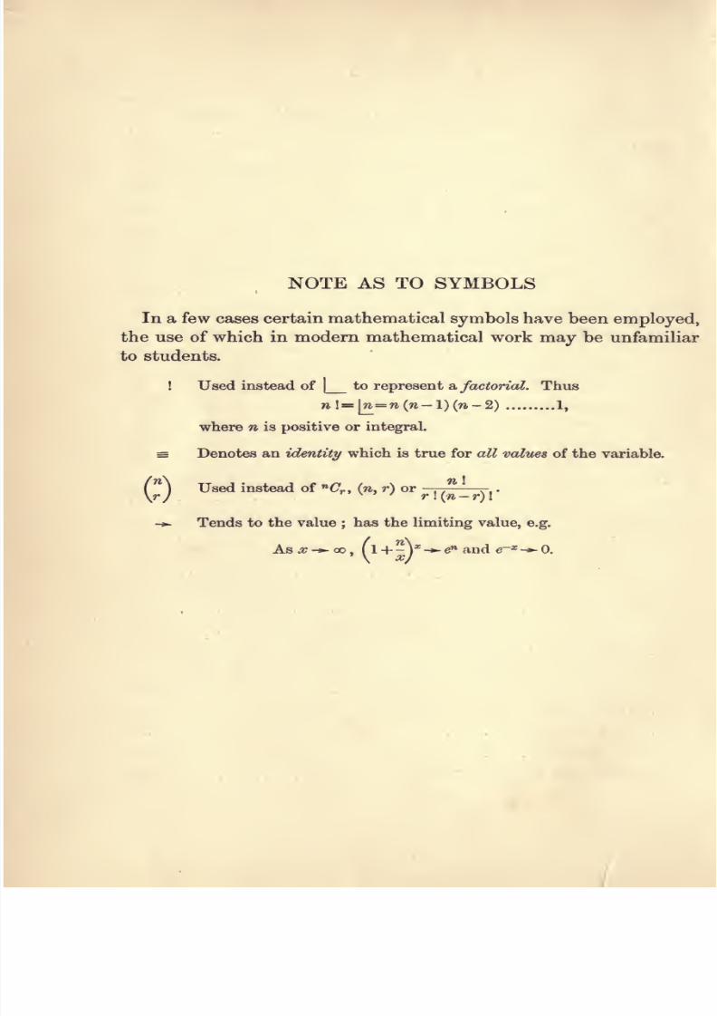
NOTE AS TO SYMBOLS
In a few cases certain mathematical symbols have been employed,
the use of which in modem mathematical work may be unfamiliar
to students.
Used instead of|
to represent & factorial. Thus
n =[71= 71(71-1) (71 -2) 1,
where n is positive or integral.
= Denotes an identity which is true for all valttes of the variable.
n\(] Used instead of C-, (n. r) or ,
rj ^ ' ' r (7i r)V
Tends to the value ; has the limiting value, e.g.
As :p -»- 00 , (1 + - r -» e and e~^ -*- 0.

7/27/2019 7-CALCULUS AND PROBABILITY-1922-Alfred Henry.pdf
http://slidepdf.com/reader/full/7-calculus-and-probability-1922-alfred-henrypdf 13/170
;e«
+ c1 '^
o) ei +
1
;>TT<J >
1 H ^
li;- S T^ -^
+ 1 I
1o
+ ^^ 52 < 3; II 'll
ii
1 lis'^
1
s^
O)
+- ^
:
^ + c?
o'tH
1-0», 1
<-)+
-§ e
9 <Hoc
5^ ^ iH1i -J.
1
++55
%a
>Ql^ +
> S <
T3
+3* S
-«
+ olc. ^-^ s ^ 1
§ '^ •tj
1—
. 1 ^ ^\^ HN «Kn
w
++
o^1 1
^ 8 «8 ^^^ /-»-.
< ^ «rs: 1—^
«ls T *^ .
g
o +k
+
1
m<
w 1—+
,^
II s ^
4-1-1 ]^ tr +
<I
o fH1
'^1
OJ
+-§
-—-^ +
Hoc
+
1
3
8+ ^ +
++
a.^.
1
1
HN S|S
rH~
«or-t
* M
od o H<-H I—
«o 1 S•g
03 •1
S
^o
9«o 00
o1—
s
^ §«o Vi i-H ^ ^ •2 H O
§«i-t ^ ,_ ^ ^
1
oo tH^ aS- W5 o ^fH04
5^ giH c- 00 a» rH
rH iH rH
iz; d ji (i d d d d d

7/27/2019 7-CALCULUS AND PROBABILITY-1922-Alfred Henry.pdf
http://slidepdf.com/reader/full/7-calculus-and-probability-1922-alfred-henrypdf 14/170

7/27/2019 7-CALCULUS AND PROBABILITY-1922-Alfred Henry.pdf
http://slidepdf.com/reader/full/7-calculus-and-probability-1922-alfred-henrypdf 15/170
CHAPTER I
FUNCTIONS. DEFINITION OF CERTAIN TERMS.
GRAPHICAL REPRESENTATION
1. When the value of a certain quantity y depends upon, or
bears a fixed relation to that of another quantity, x, y is said to be
di. function of x, and the relationship is written as y=f(x).
[Other notations used are u^-yVx, < > (x\ etc.]
Thus, we may have y — x^, y — a^, y — sin a?, y = log x. The
quantities forming the right-hand sides of the equations are all
functions of x.
When expressed in this way the relationship of y to a? is said to
be explicit But if, for example, aa^ + 2hxy + cy ^ = 0, it is clear that,
whilst the value of 3/ depends upon that of a?, it cannot be determined
in any case by direct substitution of the value of x. The relation-
ship in such circumstances is said to be implicit. In this particular
example the relationship can, of course, be made explicit by solving
the equation for y in terms of x.
The quantities x and y are called variables.
The quantity x is called the independent variable since it may
assume any value, whereas y is called the dependent variable since
its value depends upon that of x.
The independent variable is sometimes referred to as the argu-
ment
2. Functions may, of course, involve more than one variable.
For example we may have y — a?2^ ox u— ^-^; and all these
variables may be involved implicitly. A function of more than one
variable would be denoted by /(a;, y, z), vbx.yy ^tc.
If we have a function w, such that
u = aP'y^zf^ + af-'y^'sf^' + ...
and a + 6 + c = a' + 6' + c' = . . . = n,
then u is said to be a homogeneous function ofn dimensions,
H. T.B.I. 1
7/27/2019 7-CALCULUS AND PROBABILITY-1922-Alfred Henry.pdf
http://slidepdf.com/reader/full/7-calculus-and-probability-1922-alfred-henrypdf 16/170
2 .••.«. V :;.•• FUNCTIONS
-• •*-••«« <<<<< .'.•«««•••,««•••• « • •*,•««•«•§« «,*• • «f '
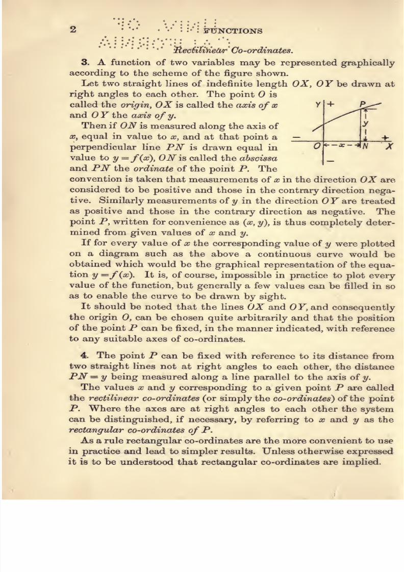
3. A function of two variables may be represented graphically
according to the scheme of the figure shown.Let two straight lines of indefinite length OX, F be drawn at
right angles to each other. The point is
called the origin, OX is called the axis of x
and Y the axis of y.
Then if ON is measured along the axis of
X, equal in value to x, and at that point a
perpendicular line
PNis drawn equal in
value to 2/= f{x), ON is called the abscissa
and PN the ordinate of the point P. The
convention is taken that measurements of x in the direction OX are
considered to be positive and those in the contrary direction nega-
tive. Similarly measurements of y in the direction OF are treated
as positive and those in the contrary direction as negative. The
point P, written for convenience as (x, y), is thus completely deter-
mined from given values of x and y.
If for every value of x the corresponding value of y were plotted
on a diagram such as the above a continuous curve would be
obtained which would be the graphical representation of the equa-
tion y =f{x). It is, of course, impossible in practice to plot every
value of the function, but generally a few values can be filled in so
as to enable the curve to be drawn by sight.
It should be noted that the lines OX and OY, and consequently
the origin 0, can be chosen quite arbitrarily and that the position
of the point P can be fixed, in the manner indicated, with reference
to any suitable axes of co-ordinates.
4. The point P can be fixed with reference to its distance fi om
two straight lines not at right angles to each other, the distance
PN= y being measured along a line parallel to the axis of y.
The values x and y corresponding to a given point P are called
the rectilinear co-ordinates (or simply the co-ordinates) of the point
P. Where the axes are at right angles to each other the system
can be distinguished, if necessary, by referring to x and y as the
rectangular co-ordinates of P.
As a rule rectangular co-ordinates are the more convenient to use
in practice and lead to simpler results. Unless otherwise expressed
it is to be understood that rectangular co-ordinates are implied.
7/27/2019 7-CALCULUS AND PROBABILITY-1922-Alfred Henry.pdf
http://slidepdf.com/reader/full/7-calculus-and-probability-1922-alfred-henrypdf 17/170
GRAPHICAL REPRESENTATION 3
5. The following examples give simple cases of the graphical
representation of explicit functions.
(i) The equation x = a clearly represents a straight line parallel
to the axis of y and at distance a from it; for the value of x at any
point is constant and equal to a.
(ii) The equation y = 7nx represents a straight line passing
through the origin and making an angle 6 with the axis of x, where
tan 6=^m\ since at any point the ratio y :x \^ constant and equal
to tan 6.
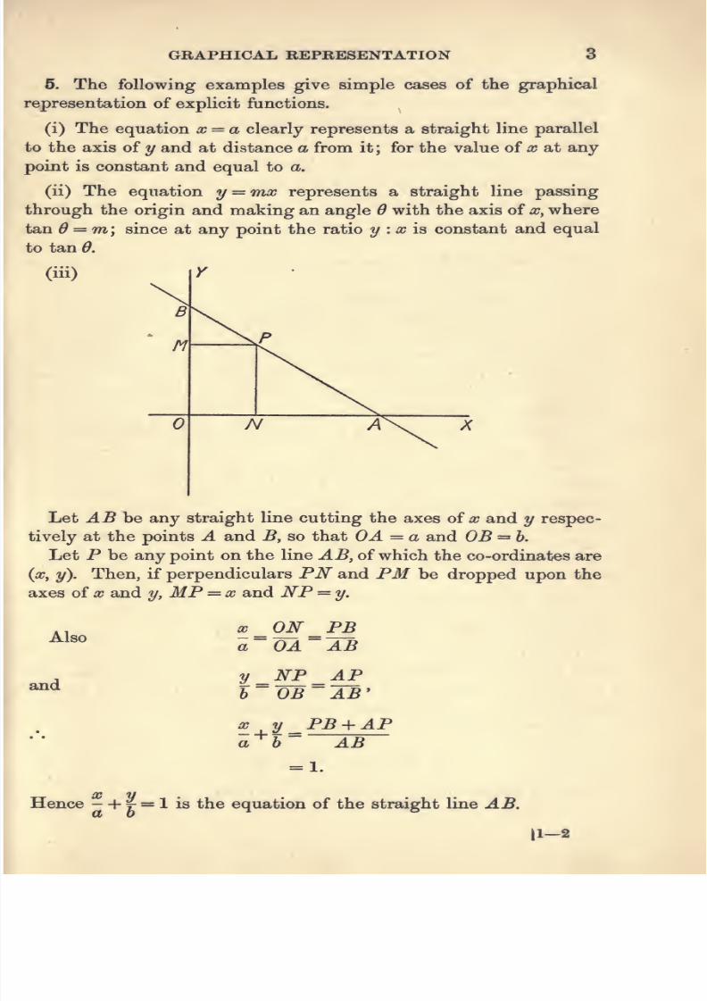
(iii)
B
M
Y
P
\s/ >l\ X
Let ilJ5 be any straight line cutting the axes oi x and y respec-
tively at the points A and 5, so that OA — a and OB = h.
Let P be any point on the line AB, of which the co-ordinates are
(a?, y). Then, if perpendiculars PN and PM be dropped upon the
axes of X and y, MP — x and NP — y.
Also
and
X ON PBa
~ 0A~~ AB
I-
NPOB
AP==AB^
X
^i-'-
^B + APa AB
= L
^ . yHence - + f = 1 is the equation of the straight line AB.
|1~2

7/27/2019 7-CALCULUS AND PROBABILITY-1922-Alfred Henry.pdf
http://slidepdf.com/reader/full/7-calculus-and-probability-1922-alfred-henrypdf 18/170
4 FUNCTIONS
6. An implicit function can be similarly represented. For ex-
ample, it is obvious from the ordinary properties of the circle that
the implicit relationship x^ + y^ — o? represents a circle of radius a
with its centre at the origin.
Note. The function y = a + hx-^ ca? -k- da? + . . . is sometimes
called a parabolic function, since the equation y^a + bx-\-cx^
is represented graphically by a curve which is known as a
parabola.
7. It does not follow that for every value ofxthere will always
be a real value of y.
Thus, consider the function y^^(x — a) (x — b)(x— c), where
c>b> a. If a; is negative, the right-hand side of the equation is
negative and y can have no real value. If x is positive and < a, the
position is the same. If, however, x> a and < 6, then the right-
hand side is positive and y has a real value; but when x>b and
< Cy y is again unreal and remains so until x>c when a real value
of y results for each value of x.
The form of the curve is shown below, where OA = a, OB = b
and 00 = c.
In circumstances such as these,
where one or more parts of a
curve are isolated from the
others, the function and the
curve representing it are said to
be discontmuous.
8. It is convenient here to
introduce the conception of the
limiting value of a function, or simply a limit.
If y=if(x) and y continuously tends towards a certain value and
can be made to differ by as little as we please from that value, by
assigning a suitable value to x, say a, then /(a) is said to be the
limiting value off(x) when x tends to the value a.
A convenient notation is as follows
y-*-f(p) when x-*-a.
Also /(a) would be expressed as Lt f(x).

7/27/2019 7-CALCULUS AND PROBABILITY-1922-Alfred Henry.pdf
http://slidepdf.com/reader/full/7-calculus-and-probability-1922-alfred-henrypdf 19/170
GEAPHICAL REPRESENTATION 5
Thus let y = . By writing y in the form 1— we see thatoc cc
by making x indefinitely great, we can make the value of y differ
from unity by as little as we please.
Thus
9. We will now give an example of another form of discontinuity,
=(—x — aj shownnd for this purpose we will take the curve y
below.
Here it will be seen that as a?-^ a, the value of y -^ oo . Similarly
if a? -*-oo, y -^1.
Thus if we draw two lines, one
PN parallel to the axis of y and at
distance a from it, and the other
QM parallel to the axis of x and at
unit distance from it, the curve will
continuously approach these lines
but will not actually touch them
except at an infinite distance from the origin.
Such lines are called asymptotes to the curve.
In general, actuarial functions are finite and continuous ; but in
mathematical work, as will be seen later, attention to these points
is necessary in the consideration of certain problems.
Y
j
v_-^^ J N ^
10. Explicit functions involving two variables, and implicit
functions of three variables, can be expressed in a diagram of three
dimensions. Thus if we have z=f{x, y) or f{x, y,z)-0 we may
measure x, y and z by reference to their perpendicular distance, not
from two lines, but from three planes at right angles to each
other.
A useful simile is that of the floor and two adjacent walls of
a rectangular room of indefinite size. Any point in space is fixed
by reference to its perpendicular distance from the two walls and
the floor, x. and y being the respective distances from the walls,
and z that from the floor. The conventions as to positive and
negative values are similar to those previously explained.

7/27/2019 7-CALCULUS AND PROBABILITY-1922-Alfred Henry.pdf
http://slidepdf.com/reader/full/7-calculus-and-probability-1922-alfred-henrypdf 20/170
FUNCTIONS
11. As an example, if ^ = x^y^, the values of the function for unit
intervals in the values of x and y are shown in the following table
Value
oft/
Value of X
1 2 3 4 ...
1
2
3
4
1
4
9
16
4
16
36
64
9
36
81
144
16
64
144
256
We will conceive the floor as being covered with a linoleum of
chess-board pattern, the sides of the squares being at unit distance
apart. The perpendicular distance from the floor of all points in
these squares is nil and, therefore, z has the value 0. The corners
of these squares will thus represent the various points (0, 0, 0),
(0, 1, 0), (1, 1, 0), (1, 0, 0), (2, 1, 0), etc. If we were to erect at each
corner a peg of height equal to the appropriate figure taken from
the above table, the tops of the pegs would give points on the surface
representing the equation z = x^y'\ If the value of z were plotted
for every possible combination of values of x and y, we should,
of course, obtain the continuous surface corresponding to z = x^y\
Polar Co-ordinates.
12. An alternative method of defining a point in a plane surface
is as follows.
Let an origin be taken and a fixed line OX be drawn fi-om it
then the position of any point P is known if the distance OP and
the angle XOP are given.
Thus if OP = r and Z XOP = 6,r and 6 are known as the polar
7/27/2019 7-CALCULUS AND PROBABILITY-1922-Alfred Henry.pdf
http://slidepdf.com/reader/full/7-calculus-and-probability-1922-alfred-henrypdf 21/170
GRAPHICAL REPRESENTATION 7
co-ordinates of P, and the point P can be written as (r, 6). The
distance OP is called the radius vector and the angle XOP is called
the vectorial angle.
The convention adopted is that the angle XOP is reckoned
positive if measured from OX in a direction contrary to that in
which the hands of a clock revolve, and negative if measured in the
reverse direction.
Further, the radius vector is considered positive if measured
from along a line bounding the vectorial angle, and negative if
measured in the opposite direction. To illustrate this system, let
PO be produced to a point Q such that 0Q = OP = r. Then the
point Q may be written alternatively as (r, tt + ^) or (— r, 6).
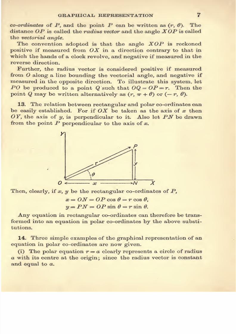
13. The relation between rectangular and polar co-ordinates can
be easily established. For if OX be taken as the axis of x then
OYy the axis of y, is perpendicular to it. Also let PN be drawn
from the point P perpendicular to the axis of x.
Then, clearly, if x, y be the rectangular co-ordinates of P,
x=: ON = OP cos e = r cos 6,
y = Pi\r = OP sin (9 = r sin 6.
Any equation in rectangular co-ordinates can therefore be trans-
formed into an equation in polar co-ordinates by the above substi-
tutions.
14. Three simple examples of the graphical representation of an
equation in polar co-ordinates are now given.
(i) The polar equation r = a clearly represents a circle of radius
a with its centre at the origin; since the radius vector is constant
and equal toa.

7/27/2019 7-CALCULUS AND PROBABILITY-1922-Alfred Henry.pdf
http://slidepdf.com/reader/full/7-calculus-and-probability-1922-alfred-henrypdf 22/170
8 FUNCTIONS
(ii) In the diagram shown in § 13, if ON = a andPN be produced
indefinitely in either direction, then the polar equation of the
straight line so obtained will be
r cos ^ = a,
since ifP be any point in the line
OP cos (9= r cos 6 = ON = a.
(iii) Let OA be a diameter of a circle OPA of radius a. Then
if P be any point on the circle such that OP = r and lAOP^Q,0P = 0A cose = 2acoad.
The polar equation of the circle, if be the origin, is therefore
r = 2a cos 6,

7/27/2019 7-CALCULUS AND PROBABILITY-1922-Alfred Henry.pdf
http://slidepdf.com/reader/full/7-calculus-and-probability-1922-alfred-henrypdf 23/170
CHAPTER II
FINITE DIFFERENCES. DEFINITIONS
1. The subject or calculus of Finite Differences deals with the
changes in the values of a function (the dependent variable) arising
from finite changes in the value of the independent variable (see
Chapter I, § 1).
Many questions arise which can be dealt with on systematic lines,
but probably the most important problems which require to be
solved in actual practice, and with which we are concerned at this
stage of the subject, are the summation of series, and the insertion
of missing terms in a series of which only certain terms are given.
It will be convenient to proceed in the first place to some ele-
mentary conceptions and definitions.
2. If we have a series consisting of a number of values of a
function, corresponding to equidistant values of the independentvariable, and from each term of the series we subtract the algebraic
value of the immediately preceding term, we shall obtain a further
series of equidistant terms. The process is known as differencing
the terms of the series, and the terms of the new series are known
as the first differences of the original terms. By repeating the pro-
cess with the terms forming the first differences, we shall obtain
afurther series forming the second differences ofthe
original function,
and so on. Thus if we have f{x) for the first term of the series
and/(a7 + ^) for the second term, the first difference oi f{x) is
f{x-\-h)-f{x) and is designated ^f{x). The second difference of
f{x) is A/ (a; + ^) - ^f(x) and is designated ^^f{x). This may be
set out as in the following scheme
Function First Differences Second Differences Third Differences
/(^)
/(^+2A)
/(^+3A)
fix+h)-fix)
f{x+2k)-fix+ h)
f{x+Zh)-f{x+ 2h)
/(^•+4A)-/(^+3A)
f{x+2h)-2f{x+h)
f{x-^3h)-2f{x+2h)
f{x+U)-2f{x+3h)+f{x+2h)
/(a:+ 3A)-3/(:r+2A)
+ 3/(^+A)-/(a;)
/(^+4A)-3/(^+3A)
+ 3/(a;+2A)-/(a;+A)

7/27/2019 7-CALCULUS AND PROBABILITY-1922-Alfred Henry.pdf
http://slidepdf.com/reader/full/7-calculus-and-probability-1922-alfred-henrypdf 24/170
10 FINITE DIFFERENCES
The first term of the series is known as the leading term and the
terms in the top line of differences are known as the leading dif-
ferences of the series.
It must be clearly understood at the outset that A is merely a
symbol representing the operation of differencing f{x) once ; it is
in no sense a coefiicient by which f{x) is multiplied. This point is
dealt with again in § 5.
3. An examination of the character of the series which ultimately
results from the process of differencing repeatedly, leads to the
development of certain important theorems. Before proceeding
further, it will be helpful to give a practical example.
Example 1. Obtain the differences of the series given hyf{x) = af^,
where x has all integral values from 1 to 6.
/(^)Firpt Second Tliird Fourth
Differences Differences Differences Differences
1 1 7 12 6
2 8 19 18 6
3 27 37 24 6
4 64 61 30
5 125 91
6 216
It will be observed in the above example that the fourth and,
therefore, all higher differences are zero ; it will be seen later that
this would equally have been the case had more terms of the series
been taken. We can therefore construct all the remaining terms
of the series by a process of continuous addition.
4. Although most functions with which the actuary has to deal
are not of the simple character of that shown above, yet it will
usually be found that the differences of the function for which
further values are required tend to the value zero and are sus-
ceptible to treatment by methods which will be developed subse-
quently.
The student should obtain confirmation of this fact and insight
into the character of certain series by taking out the differences of
tabulated functions such as logarithms, annuity-values, etc.

7/27/2019 7-CALCULUS AND PROBABILITY-1922-Alfred Henry.pdf
http://slidepdf.com/reader/full/7-calculus-and-probability-1922-alfred-henrypdf 25/170
DEFINITIONS 11
5. Before proceeding to the consideration of the various problems
which arise, it is necessary to develop certain fundamental formulas.
In § 2 A has already been defined as the symbol of the operation
by means of which the value of f(x + h)—f{x) is obtained.
Similarly, it is customary to use the symbol E as representing
the operation by which the value of /(a?) is changed to the value
f{(c + A), so that
Ef{x) =/(^ + h) =f(x) + Af(x).
It must be carefully remembered that these symbols represent
operations only and must be interpreted accordingly. Thus E^a^ is
clearly not the equivalent of (Exf; the former expresses the result
of operating twice upon the function xf^ in the manner indicated
above, giving a value (x + 2hy, whereas in the latter case the opera-
tion is applied once to the function x and the resulting term (x + h)
is squared.
6. If, then, these symbols are found to obey the ordinary alge-
braical laws, they can be dealt with algebraically provided always
that the results are interpreted symbolically in relation to the
function which is the subject of the operation. This principle is
known as that of Separation of Symbols or Calculus of Operations.
The algebraic laws referred to above comprise
(1) The Law of Distribution.
(2) The Law of Indices.
(3) The Law of Commutation.Taking these laws in succession
(1) The symbol A is distributive in its operation, for
= [/i (x+h) -AW] + [/s (^+ h) -/, (x)]
+ [A(^ + h)-Mx)]-h...
= A/(a;) + A/,(^) + A/3(a;)-H....
Similarly the symbol E is distributive, for
£ [Ma:)-\-A{x)+Mx)+...]^[f,(x + h)+Mx-hh)^Mx-\-h)+...]
==EMx) + EMx)-^EMx)-\-....
(2) The symbol A obeys the law of indices, for in the case of
positive integers the symbol A '/ (a;) represents the operation,
repeated m times, of differencing f(x).

7/27/2019 7-CALCULUS AND PROBABILITY-1922-Alfred Henry.pdf
http://slidepdf.com/reader/full/7-calculus-and-probability-1922-alfred-henrypdf 26/170
12 FINITE DIFFERENCES
Thus A »/(a;) = (AAA ... m times)/(a;),
.-. A'»A */(a;) = (AAA ...n times) (AAA . . . m times) /(a;)
= (AAA . . . (m + 7i) times) /(a?)
= A + »/(a;).
Similarly it may be shown that the symbol E obeys the law of
indices.
(3) The symbol A is commutative in its operation as regards
constants, for, if c be a constant,
A[cf(x)] = c/(x + h)-cf(x)
^cAf(x).The like result can be deduced as regards E.
7. It follows that, since
Ef{x) = (l-^A)f(x),
therefore E= l+Aand A = J5;-1.
The two operators are thus connected by a simple relation, which
will be found later to lead to important results.
8. As an example of the manner in which the relationship
between the operations represented by E and A can be utilised in
the solution of problems, we may take the following
Example 2. Prove that
/(0) + ^/(l) + J/(2) + g/(3) + ...
= ^ [/(O) + a;A/(0) +J AV(0) +...].
Since
/(I) = E/(0) = (1 + A)/(0); /(2) = E'/(0) = (1 + A)V(O), etc.,
we have /(O) + xf(l) +J/(2)
+J /(3) + J.
= [l +^(1 + A) + |-J(l + A)« + ...]/(0)
= [«' +''>]/(0)
= e-[e-^]/(0)
/(O)A'
l+xA + a^j^ + ..
/(0)+^A/(0) + jAy(0)+...].
7/27/2019 7-CALCULUS AND PROBABILITY-1922-Alfred Henry.pdf
http://slidepdf.com/reader/full/7-calculus-and-probability-1922-alfred-henrypdf 27/170
CHAPTER III
FINITE DIFFERENCES. GENERAL FORMULASAND SPECIAL CASES
1. Starting from the relationship proved in Chapter II, § 7, it is
now possible to develop two formulas of the utmost importance.
2. To express /(a; + mh) in terms of f(x) and its leading dif-
ferences.
By definition f(a) + mh) = E^f(x)
= (l + A)-/(^),
since by Chapter II, § 7, ^ = 1 + A.
Expanding the above expression by the Binomial Theorem we
have
/(a, + mA) = [l + mA + (™) A^ +(;:)
A»+ . . . + (^ A^'jfix)
=/(«:) + m^f(a^) + (^) AV(a.) + Q) A'f(cc) + ...
+ C)^ '/W (D-
Bearing in mind that the symbol A obeys the ordinary algebraic
laws and that the Binomial Theorem holds for all values of the
index, positive, fractional or negative, it will be realised that the
above proof is perfectly general.
It is instructive, however, to show how the formula may be
deduced for fractional and for negative values of m.
3. Fractional value. Let — be a positive proper fraction, and
let the interval between the given terms of the series be h. It is
required to find the value of f(x-^—h].
Also let f(x + h) -f(x) = A/(a;),
and /(^ + J)-/W = VW.
7/27/2019 7-CALCULUS AND PROBABILITY-1922-Alfred Henry.pdf
http://slidepdf.com/reader/full/7-calculus-and-probability-1922-alfred-henrypdf 28/170
14 FINITE DIFFERENCES
In the second case, the unit of differencing has been altered to
- and, bearing in mind that n is a positive integer, we may write
at once from the theorem in the preceding article
therefore (1 + A)/(^) = (1 + Byf(x\
and (1 + ^ff(x) = (1 + B)f(x).
Since m is also an integer, it follows that
(1 + Srf(x) =/
(a; +^
a) = (1 + A)V(^)
=/(^)+^ Af(w) + AY(x)+ . ..
4. Negative value. It is desired to find the value oif{x — mh).
Now, from the preceding theorems, it is clear that
i\ + ^rf{x-mh)^f{xltherefore
/(a;-TOA) = (l + A)- '/W
= [l + (-m)A + (-^)A'+. ..]/(:.)
=/(^) +(-m)A/W + (-;)AV(«)+....
The above proofs show that the theorem holds universally and
illustrate how the principle of Separation of Symbols can be applied
whenever the symbols of operation obey the ordinary laws of algebra.
5. To express A^f(x) in terms of f(x) and its successive values.
A-^f{x) = (E-irf(x)
= [^ » - mE' -- ^ +(2 )
^ ^' -...+(- ) »] f(x)
=/(a; + mh) - mf(x + ^^T^lA) + ( 2 )/(^ + m-2A) -. .
+ (-l)-/W (2).
Alternatively both the above formulas can be easily proved by
the ordinary methods of induction.
Formula (1) also follows directly from the ordinary formula of
Divided Differences (see Chapter VIII). This method has the
advantage of showing directly the application of formula (1) to cases
where m has a fractional or a negative value.

7/27/2019 7-CALCULUS AND PROBABILITY-1922-Alfred Henry.pdf
http://slidepdf.com/reader/full/7-calculus-and-probability-1922-alfred-henrypdf 29/170
GENEBAL FORMULAS AND SPECIAL CASES 15
6. The above formulas are expressed in a form which applies in
the most general way, i.e. when the interval of differencing is h and
the leading term is /(a?). It is clear, however, that by altering the
unit of measurement the formula will be simplified although the
result is not affected. Similarly by changing the leading term
(which process corresponds to shifting the origin ) so that the
leading term is expressed as /(O) a further simplification in form
is made.
If, therefore, the interval of differencing becomes unity and the
leading term can be represented by /(O), the first formula can be
written
/«=/(0) + nA/(0)+(2)AV(0)+ (3).
An example will make this clear.
Having given the values of/(10), /(15),/(20), etc. it is desired
to express /(17) in terms of /(lO) and its leading differences.
The original formula (1) gives the value of /(lO + 1'4A), where
A = 5, and therefore we write
/(lO + 1'4A) =/(10) + 1-4A/(10) + ^-i^^^^AV(lO) 4- ...
where A, A'^, ... are taken over the interval h.
But the same result is secured if the unit of measurement is
changed from 1 to 5 and if at the same time /(lO) is made the
initial term of the series, for then /(lO), /(lo), /(20), ... can be
written as^(0),
F{1), F(2), ... and the required value, viz./(l7),
becomes F(l'4i) which by formula (3) is equal to
i^(0) + 1-4AF(0) +^^^^^ A'^i^CO) + ....
7. The above formulas are of general application if sufficient
terms of the series are known, but it is convenient at this stage to
consider the particular forms taken by the differences of certain
special functions.
8. f{x) = ax^
The result of differencing has been, therefore, to change the term
involving the highest power of so from ax^ to anx ^'^ (thus reducing
its degree in x).

7/27/2019 7-CALCULUS AND PROBABILITY-1922-Alfred Henry.pdf
http://slidepdf.com/reader/full/7-calculus-and-probability-1922-alfred-henrypdf 30/170
16 FINITE DIFFERENCES
Similarly a further process of differencing will reduce the degree
of a; to n — 2 and the coefficient of the highest power of x will be
an (n — 1). By repeating the process we arrive at the result that
the nth difference of ax ^ is independent of x and is equal to a.n\.
The (n + l)th difference is therefore zero.
Corollary. It follows that the nth difference of
ax'^-\-bx'^^ + cx'^-^+ ... +k
is constant and equal to a . w .
9. f(x) = X (x - 1) (x - 2) ,.. (x - m -\^ 1).
This expression is usually denoted by x^*^\
Af(x)^(x+l)x(x-l)...(x'-m + 2)-x(x-'l)(x-2)...(x-m+l)
= mx (x—l),..(x — m + 2)
— 'mx^^~^\
Similarly Ay (a?) = m (m - 1) a;^ ^^)^
By repea,ting the process we arrive at the result
A */(a;) = m ,
which is otherwise obvious from the preceding article since /(a?) is
of the 7^ith degree in x,
10. f{x) =^ (^ + 1) (^ ^ 2) . . . (a; + m - 1)
•
Corresponding to the notation already used, this can be denotedby ajt-* ).
^^^^^ (a;+l)(a? + 2)...(a? + m) x{x-\-l){x-\-2) ...(x + m-\)
— ma; (a? + 1) (ic + 2) . . . (a? + m)
= — 77ia;^~ *+^^
Similarly Ay(a;) = m (m + 1) a;(-^»+>)
and so on.
11. /(^) = a^
A/ (a:) = a*+i - o*
= a*(a-l).
Whence Ay(a?) ^a'^ia- ly.

7/27/2019 7-CALCULUS AND PROBABILITY-1922-Alfred Henry.pdf
http://slidepdf.com/reader/full/7-calculus-and-probability-1922-alfred-henrypdf 31/170
GENERAL FORMULAS AND SPECIAL CASES 17
12. For many purposes it is convenient to have a table of the
leading differences of the powers of the natural numbers. These
can be represented as the differences of [aj*»]a,=o and are sometimes
known as the Differences of 0.
The following table gives a number of values of the first term
and leading differences of l^'^x^]x=o, which, for convenience, can
be written as ^ ^O'*
n /(O) A A2 A3 A4 A6 A«
1
2 2 —3 6 6 —4 14 36 24 —5 30 150 240 120
13. A working formula for constructing a table such as the
above by a continuous process may be obtained as follows:
[See formula (2).]
Therefore, when f(x) — x^,
whence, puttinga?
= 0,
= n [n* - - (n - 1) (n - l)'^-i + ( ^2 ^) (71 - 2) *-^ - . .
.]
= w [(1+ n-Vf-'^ - (w - 1) (1 4-^ir:2)^-i
= 71 [A«-ia; »-i]a.=i (4).
But /(l)=/(0) + A/(0),
and A'^-^/ri) = A'^-i/(0) + AV(0).
Therefore
[^n-i^w-i]^^^= [A -iar »-i]x=o + [A a;^-^J„=o
H. T.B.I.

7/27/2019 7-CALCULUS AND PROBABILITY-1922-Alfred Henry.pdf
http://slidepdf.com/reader/full/7-calculus-and-probability-1922-alfred-henrypdf 32/170
18 FINITE DIFFERENCES
Hence A'»0»»» = n [A^-^O^^^ + A'^O *- ] (5).
It follows that the differences of [oj'^Jajrro can be constructed from
those of [x^~%^Q, and soon.
To take an example from the table given above,
A*0» = 4[A»0*4-A*0^]
= 4 [36 + 24] = 240.
14. By using the result given in § 9, it is possible to expand
f(x) in terms of ic<°^ x^^\ x^^\—Let f(x) = ilo + ^loo^'^ + ^aa^^'^ + ^sa;^'^ +
• • • •
Then, putting a; = 0, we' see that
/(0) = A.
Differencing both sides of the equation, we get
Af(x) = A, + 2A,x^'^ + SA,x^'^ + . . .
Again putting a; = 0, we find
A/(0) = ^,.
By repeating the above processes, we obtain successively
Ay(0) = 2 ^, AV(0) = 3 .l3,... AY(0) = n ^„,
whence
A=/(0), A = A/(0). A =^4f->....
A.=^,and
f(x) =/(0) + xAfiO) +J A»/(0) + ... +5 A»/(0) + ... (6).

7/27/2019 7-CALCULUS AND PROBABILITY-1922-Alfred Henry.pdf
http://slidepdf.com/reader/full/7-calculus-and-probability-1922-alfred-henrypdf 33/170
CHAPTER IV
FINITE DIFFERENCES. INTERPOLATION
1. The subject of interpolation is one of the most important in
Finite Differences and may be enunciateid as follows.
It frequently happens that we have given a number of values of
f{x) corresponding to different values of x, and we wish to find
a value of the function for some other value of x. If the form
of the functionis
knownor
can be deduced from the given values,the problem is, of course, simple, although in many cases it is more
convenient to proceed by the methods of Finite Differences. But it
is frequently the case, especially in actuarial work, that the function
cannot be expressed, algebraically or otherwise, in any simple form,
and resort must be had to other devices.
2. Looked at from the point of view of a problem in graphs, we
may regard the given values of the function as representinga numberof isolated points on a curve, and it is desired to plot a further point
corresponding to a given value of the abscissa.
It follows that if the form of the function (i.e. the equation of
the curve) is unknown, some assumption must be made as to the
relationship between the different values. The formulas of finite
differences assume that this relationshipcan be expressed in the form
y=^a-\-hx + cx^-\-dc(^+ ... ^kx^'K
This assumes (see Chapter III, § 8) that all orders of differences
higher than the {n — l)th vanish, but, as pointed out in Chapter II,
§ 4, this assumption can be made without introducing important
errors in practically all cases where actuarial functions are involved.
3. The above equation contains n constants, and therefore n
values of the function must be known if the values of the constants
are to be determined. Conversely, if n values only are known and
the methods of finite differences are to be applied, it must be
assumed implicitly that all orders of difierences higher than the
rn — l)th vanish.
4. The most obvious method of procedure is to obtain the n
equations given by the n values of the function and to find the
values ofthe constants therefrom. The assumed form of the function
Sl-2

7/27/2019 7-CALCULUS AND PROBABILITY-1922-Alfred Henry.pdf
http://slidepdf.com/reader/full/7-calculus-and-probability-1922-alfred-henrypdf 34/170
20 FINITE DIFFERENCES
is then completely determined and the value corresponding to any
value of X can be obtained.
In the majority of cases, however, this is not the most simple
method of working, for other devices can be adopted which will
materially shorten the arithmetical work. It is important to note,
however, that alternative formulas, in which the same values of the
function are used, lead to identical results.
In some cases there is scope for the exercise of the ingenuity of
the solver, but usually the problems fall into the main categories
which are illustrated in the following examples.
5. Example 1. When n equidistant values ofa function are given
and it is required to find the valueofsome intermediateterm or terms.
This can be done readily by the application of formula (1) of
Chapter III, or by the simpler formula (3). From the given values
the successive orders of differences are calculated, and the result is
obtained by direct substitution.
Thus, taking the numbers living by the H^ table at ages 45,
60, 55, 60 and 65, it is required to find the value for age 57.
In conformance with formula (3) the given values can be denoted
by/(0),/(l), ..., so that the required value is/(2-4). Then
/(2-4) =/(0) + 2-4 A/(0) + ?^i|^^Ay(0)
24
The working is as follows:
X /(^) A/(x) AV(^) A3/(x) AV(^)
1
2
3
4
77918
72795
66566
58842
49309
-5123
-6229-7724-9533
-1106-1495-1809
-389-314
+ 75
From above:
/(2-4) = 77918 + 2-4 (- 5123) + 1-68 (- 1106)
+ -224 (- 389) - -0336 (+ 75)
= 77918 - 12295-2 - 18581 - 87*1 - 25
= 636751.
The value given by the table is 63677.

7/27/2019 7-CALCULUS AND PROBABILITY-1922-Alfred Henry.pdf
http://slidepdf.com/reader/full/7-calculus-and-probability-1922-alfred-henrypdf 35/170
INTERPOLATION 21
The difiference between the interpolated value and the true value
is due to the fact that the interpolation curve, which is based on
the assumption that all differences of higher order than the fourth
vanish, represents only approximately the true function.
6. Example 2. When the values given and the value sought
constitute a series of equidistant terms.
If there are n terms given of which n — 1 are known, then, as
explained in § 3, it must be assumed that the {n — l)th order of
differences is zero.
Thus, using formula (2) of Chapter III, we have
A—/(0) = 0=/(«-l)-(«-l)/(H-2)+( -')/(n-3)-...
+(-i) -7(0).
In this equation there is only one unknown quantity and its
value can, therefore, be readily obtained.
For example, if
/(0)= log 3-50 = -54407,
/(I) = log 3-51 = -54531,
/(2) = log 3-52 = -54654,
/(4) = log 3-54 = -54900,
and it is required to find log 3*53, i.e./(3).
From above:
AV(0) = =/(4) - 4/(3) + 6/(2) - 4/(1) +/(0),
whence f^^^Ji^)^m^)-¥il)^m= -54777,
which agrees with the true value to five decimal places.
7. Example 3. If more than one term is missing from the com-
plete series, a somewhat similar process may be followed. Thus, if
two terms are missing, only {n—2) terms are known and the (w— 2)th
order of differences must be assumed to vanish. It is then possible
to construct two equations:
An-./(0) =/(n _ 2) - (71 - 2)/(n - 3) 4- . . . + (- 1)~-»/(0) = 0,
A--/(l)=/(;i-l)-(7i-2)/(n-2) + ...+(-l)--«/(l) = 0.
From these equations, the values of the two unknowns can be
calculated.
Similarly if a larger number of terms is missing, the method
can be extended.

7/27/2019 7-CALCULUS AND PROBABILITY-1922-Alfred Henry.pdf
http://slidepdf.com/reader/full/7-calculus-and-probability-1922-alfred-henrypdf 36/170
22 FINITE DIFFERENCES
8. Example 4. If several equidistant values are given, together
with one isolated term.
For instance, if three values /(O), /(I) and /(2) are given, to-
gether with a further value f{h). Having four values of the function
it must be assumed that the fourth order of differences is zero and
it remains to find the values of the other three leading differences.
The first two leading differences are obtained at once by differencing
the first three terms of the series, and the value of the third dif-
ference is then given by the equation
m=/(0)+ AA/(0)+ (*) A«/(0) + (*) Ay(0).
For example, taking the numbers living by the H^ table at ages
45, 46, 47 and 50, it is required to find values for ages 48 and 49.
A A«
-954 -32
-986
/(0) = 77918
/(I) = 76964
/(2)=: 75978
/(5) = 72795
/(5) =/(0) + 6A/(0) + 10A7(0) + 10A'/(0),
^,y (0)= /(5)-[/(0) + 5A/(0)^10A7(0)]
_ 72795 - [77918 - 4770 - 320]
10= -3-3.
The table is then completed by addition. Thus:
Age
X /(^) A A2 A3
45 77918 - 954 -32 -3-3
46 76964 - 986 -35-3 -3-3
47 75978 - 1021-3 -38-6 -3 3
48 74956-7 - 1059-9 -41-9
49 73896-8 -1101-8
50 72795-0
The work is checked by the reproduction of the value for age 50.
The tabular values for ages 48 and 49 are 74957 and 73896
respectively.

7/27/2019 7-CALCULUS AND PROBABILITY-1922-Alfred Henry.pdf
http://slidepdf.com/reader/full/7-calculus-and-probability-1922-alfred-henrypdf 37/170
INTERPOLATION 23
Values precisely the same as those obtained above would have
been given if the two missing terms had been inserted by the
method described in Example 3. It is instructive to confirm this
by actual calculation and to compare the two methods of procedure.
9. Example 5. Subdivision of Intervals.
This problem arises when a series of equidistant terms of a series
is given (usually every fifth term or every tenth term) and it is
desired to find by interpolation the values of all the intermediate
terms.
The simplest method of procedure is to calculate from the given
values the differences corresponding to the individual terms of the
series (the subdivided differences) and thence to construct the table
by summation. The calculation is checked by the reproduction of
the values of the original terms.
Thus assume that the given terms are /(O), /(I), .../(5) and it
is desired to complete the series /(O), /(i), /(f), etc. It is con-
venient to adopt the notation
/(l)-/(0) = A/(0),
and /a)-/(0) = 8/(0).
The problem then becomes to express Bf (0), 8 / (0), ... in terms
ofA/(0),Ay(0)
Writing y (1), /(2), ... in terms of the subdivided differences,
/(0)= /(0)/(l)=/(0)+ 58/(0)+ 10S2/(0)+ 1083/(0)+ 584/(0)+ 8^/(0)
/(2)=/(0) +
108/(0)+ 4582/(0)+ 12083/(0)+ 2108^/(0)+ 2528^/(0)
/(3)= /(0) + 158/(0)+ 10582/(0)+ 45583/(0)+ 13658^/(0)+ 30038^/(0)
/(4) = /(0) + 208/(0) + 19082/(0) + 114083/(0)+ 48458V(0) + 1550486/(0)
/(5)= /(0) + 258/(0)+ 30082/(0) + 2300S3/(0) + 1265084/ (0)+ 5313086/(0)
Differencing successively both sides of the equation, we have
A/(0)= 58/(0)+ 1082/(0)+ 1083/(0)+ 58^/(0)+ 8^/(0)
A/(l)= 58/(0)+ 3582/(0)+ 11083/(0)+ 2058^/(0)+ 2518^(0)
A/(2)= 58/(0)+ 6082/(0)+ 33583/(0) + 11558^/(0)+ 275186/(0)
A/(3)= 58/(0)+ 8582/(0)+ 68583/(0) + 34808^/(0)+ 125018^/(0)
A/(4)= 58/(0)+ 11082/ (0) + 1160S3/(0)+ 780584/(0)+ 3762686/(0)
a2/(0)= 2582/(0)+ 10083/(0)+ 2008y(0)+ 2508^/(0)
a2/(1)= 2582/(0)+ 22583/(0)+ 95084/ (0)+ 25008^/(0)
a2/(2)= 2582/(0)+ 35083/(0) + 2325SY(0)+ 97508^/(0)
a2/(3)= 2582/(0)+ 47583/(0) + 432584/(0)+ 25125S6/(0)
A3/(0)= 12583/(0)+ 75084/(0)+ 22508^/(0)
A3/(1)= 12583/(0)+ 137584/(0)+ 72508^/(0)
a3/(2)= 12583/(0)+ 200084/(0)+ 153758^/(0)
a4/(0)= 62584/(0)+ 500085/(0)
A4/(1)= 62584/(0)+812586/(0)
A6/(0)= 312586/(0)

7/27/2019 7-CALCULUS AND PROBABILITY-1922-Alfred Henry.pdf
http://slidepdf.com/reader/full/7-calculus-and-probability-1922-alfred-henrypdf 38/170
24 FINITE DIFFERENCES
Whence the values of Bf(0\ 8^(0), ... B'f(0) can readily be
obtained.
10. Alternatively the formulas for S, B\ ... can easily be written
down by using the method of Separation of Symbols.
Thus (1 + Syf (x) = (1 + A)/ (cc).
Therefore (1 + 5)/ (a?) = (1 + A)^ / (x),
and S/(^) = [(l + A)^-l]/(^)
= [-2A - -08 A=^ + '04>8A'...]f(x).
Hence ^Vi^) = ['2A - '08 A^ + -048A^...]^f (x)
= [-04A»- -032 A« + -0256 A* ...]/(«;)
and so on.
For convenience the coefficients of A, A*, . . . occurring in the
values of B, 8^ ... are given, for the intervals 5 and 10, in the fol-
lowing tables.
Subdivision into 5 intervals
Value of
Coefficient of
A A» A3 A* A»
d
8*
86
+ •2 -•08
+ -04
+ •048
-•032
+ •008
- -0336
+ •0256
-•0096+ ^0016
+ ^025536
-•02112
+ -00960- -00256
+ -00032
Subdivision into 10 intervals
Value of
Coefficient of
A A2 A3 A* A»
8
82
83
84
8^
+ -1 --045
+ •01
+ -0285
-•009
+ •001
- -0206625
+ -007725
- -00135
+ •0001
+ •01611675
- ^0066975
+ ^0014625
- •ooois
+ •00001

7/27/2019 7-CALCULUS AND PROBABILITY-1922-Alfred Henry.pdf
http://slidepdf.com/reader/full/7-calculus-and-probability-1922-alfred-henrypdf 39/170
INTERPOLATION 25
11. The following example gives an illustration of the method
of working.
Given the present values, at 3 per cent, interest, of an annuity of
1 per annum for 20, 25, . . . 45 years, it is required to find the inter-
vening values.
We have
X f{^) A A2 A3 A* A5
20 14-8775 2-5356 - -3483 •0478 -•0065 •0007
25 17-4131 2-1873 --30O5 •0413 --005830 19-6004 1-8868 - -2592 -0355
35 21-4872 1-6276 - -2237
40 23-1148 1-4039
45 24-5187
Applying the factors given in the former of the above tables, we
have
¥(20) = [•2A - •08A=' + •048A3 - 'OSSGA^ 4- •025536A»]/(20)
= -2 X 2-5356 + -08 x -3483 + '048 x 0478 + -0336 x -0065
4- -025536 X -0007
= •5375146752.
g<=- -000012192,
p = -000000224.
Similarly
S2 = _ -015642784,
B' = -000451520,
The table is then constructed by addition from these leading
differences as shown below.
It is necessary to consider how many decimal places should be
retained in the working. This depends, in the first place, on the
degree of accuracy desired in the result. Thus if four decimal
places are required in f{ai), our result must be given to at least
one place more. Further, the range of the formula is 25 terms, and
in the final term the values of S, 3^, ... S** are multiplied respectively
^y(i)' (2)' ---(s)'which are respectively equal to 25, 300,
2300, 12650, 53130. In view of the magnitude of these coefficients,
we shall need to retain at least six decimal places more in the value
of 8° than are required in the final value of /(a;). Since the co-
efficients of the lower orders of differences are smaller than 53130,

7/27/2019 7-CALCULUS AND PROBABILITY-1922-Alfred Henry.pdf
http://slidepdf.com/reader/full/7-calculus-and-probability-1922-alfred-henrypdf 40/170
26 FINITE DIFFERENCES
a correspondingly smaller number of decimal places can be retained.
In practice, however, there is little to be gained by cutting down,
unless only a rough result is required.
The working of the first five terms in the example is shown
below. It will be noticed that the accuracy of the work up to this
stage is checked by the exact reproduction of the value of /(25).
The interpolated values agree exactly with the true values to four
places of decimals.
X /(^) d (58 83 5* 5°
20 14-8775 •5375147 - -01564278 •000451520 -•000012192 -000000224
21 15-415015 -5218719 1519126 439328 11968 224
22 15-936887 •5066806 1475193 427360 11744 224
23 16-443568 •4919287 1432457 415616 11520 224
24 16-935497 •4776041 1390895 404096 11296 224
26 17-413101 •4636951 1350485 392800 11072 224
12. Example 6. Lagrange's Theorem.
We have now to consider the construction of an interpolation
formula which will apply when the given terms of the series are
not equidistant.
Let n values of the function be given, namely
/(a),/(6)./(c)..../(n).
Then the function must be assumed to be a parabolic function of
X of degree (n — 1). (See § 3.) Assume therefore that the function
can be represented as
f(x) = A{x'-b)(x-c) ...(x — n)
-\- B {x-^a){x — c) ...{x — n)
+ C (x — a) (x — b) . . . (x — n)
+ etc.,
there being n terms in all, each composed of (n — 1) factors multi-
plied by a constant, the values of the constants having yet to be
determined. It is clear that the right-hand side of the equation
is of degree (n — l).
To find the values of the constants we proceed as follows:
Put x = a.
Then /(a) = ^(a-6)(a-c) ... (a - n-).

7/27/2019 7-CALCULUS AND PROBABILITY-1922-Alfred Henry.pdf
http://slidepdf.com/reader/full/7-calculus-and-probability-1922-alfred-henrypdf 41/170
Therefore A=^
INTERPOLATION 27
f{o)
(a — b)(a — c) . . .{a — n)*
Similarly ^ = (b -a){b-c)...(b-ny
and so on.
Substituting these values of ^, jB, ... in the original equation
we have
fr^\ - f(n\(a?-6)(a?-c)...(^-n) , {x-a){x-c)..,{x-n)
(x-a){x-h)(x-c)..,^ '^J^''\n-a)in-h){n-c)... '^^^'
By an obvious transformation, the formula can be put in a some-
what simpler form for calculations, namely
/(^) fi^{x-a){x-h)...{x-n) {x - a) (a -h){a- c) .., (a- n)
/(6) /(ri)
'^(b-a){x-b),,.{b-n)'^ ''^{n-a)(n-b){n-c)..,(x-n)
(2).
In memorising the formula it should be noted that the denomi-
nators are made up of the product of the algebraic differences of
the values of the variable, the term {a — a) being replaced by (x — a)
and so on.
13. The formula is somewhat laborious to apply, and careful
attention to signs is required, but it is convenient to use where only
one or two unknown values of the function are required. Since the
assumptions underlying it are precisely similar to those previously
explained, its use in any particular case will give identical results
with those which can be obtained by the use of the ordinary
methods of Finite Differences where a sufficiently high order of
differences has been taken into account.
To illustrate this point and to provide an example of the use
of the formula, we will calculate by Lagrange's formula the value
for age 49 in Example 4. In this case we have
/(0) = 77918, /(I) = 76964, /(2) = 75978, /(5) = 72795,
and it is required to find the value of/(4).

7/27/2019 7-CALCULUS AND PROBABILITY-1922-Alfred Henry.pdf
http://slidepdf.com/reader/full/7-calculus-and-probability-1922-alfred-henrypdf 42/170
28 FINITE DIFFERENCES
We have accordingly
/(4) /(O)
(4_0)(4-l)(4-2)(4-5) (4-0)(0-l)(0-2)(0-5)
/(I) /(2)+ (l-0)(4-l)(l-2)(l-5) + (2~0)(2-l)(4-2)(2-5)
,
/(5)
^(5-0)(5-l)(5-2)(4-6)*
or, - ,V/W = - A/(0) + ^f(l) - A/(2) - fV/(5).
Whence we find/(4) = 73896*8, as before.
It should be noted, as a check on the formula, that the sum of
the coefficients of the terms on the right-hand side of the equation
must equal the coefficient of the term on the left-hand side of the
equation.
14. Problems of interpolation between terms at unequal inter-
vals can also be dealt with in a simple way by the formulas of
Divided Differences (see Chapter VIII).
7/27/2019 7-CALCULUS AND PROBABILITY-1922-Alfred Henry.pdf
http://slidepdf.com/reader/full/7-calculus-and-probability-1922-alfred-henrypdf 43/170
CHAPTER V
FINITE DIFFERENCES. CENTRAL DIFFERENCES
1. It has already been stated that in interpolating between given
values of a function the form of the expression connecting these
values is assumed to be parabolic, and that this assumption is usually-
only an approximation to the truth. It remains therefore to beconsidered by what methods the best result can be obtained by the
processes of Finite Differences.
2. In developing the formulas of this chapter, it will be assumed
that a number of equidistant values of the function are given.
Let us assume further that it is desired to interpolate a value /(a?)
intermediate between /(O) and /(I). It is clear that our knowledge
of the shape of the curve on which the points lie is increased if we
are given values of the function lying on both sides of /(O), and
that generally the best value of /(a?) will be obtained, if a limited
number of terms is to be used, when the required value occupies
as nearly as possible a central position in regard to the terms used
in the interpolation.
The formulas of Central Differences are designed to give effect
to these considerations.
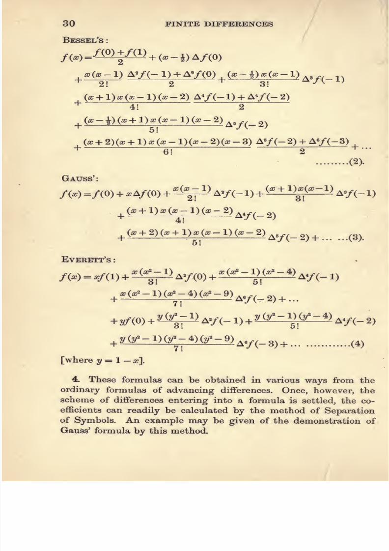
3. The more familiar formulas of Central Differences are as
follows
Stirling's :
x(^-l) A»/(- 1) + A'/(- 2) ai'ix'-l) . .
+ 3j 2^ 4 ' '
x(_a^-l)(a^-4,) A'/(- 2) + A'/(- 3)• 52
^^(^-l)(^-4)
^.^^_3^^ (1).
7/27/2019 7-CALCULUS AND PROBABILITY-1922-Alfred Henry.pdf
http://slidepdf.com/reader/full/7-calculus-and-probability-1922-alfred-henrypdf 44/170
30 FINITE DIFFERENCES
Bessel's :
/W=-^^^^> + (-i)A/(0)
.x(x-l) A'f(-l) + ^'f(0) (x-i)x(x-l)2 2 3
•'^
,
(x+ l)x{x-l)(x-2) A'f(-l)+ A'f(-2)*4 2
_^(a;-|)(a: + l)a;(a;-l)(a:-2)
^.^^_ ^^
.
(a;
+2)(a;
+l)a;(a;-l)(g-2)(a -3) A'/(-2) + A«/(-3)
* 6 2 ^'(2).
Gauss':
fix) =/(0) + ^A/(0) +?^> A'/(-l) + (^ + iy-l) A»/(-l)
o
Everett's :
f{x) = »/(i) +^<^ A»/(0)'^(^-iK^-4)Ay(- 1)
+a^(0)+^-^Ay(-i)+y^y'-y^'-^)
Ay(-2)
^y(y^-l)(y»^-4)(y^-9)^y^_3^^^^^
[where y = 1 - a?].
4. These formulas can be obtained in various ways from the
ordinary formulas of advancing differences. Once, however, the
scheme of differences entering into a formula is settled, the co-
efficients can readily be calculated by the method of Separation
of Symbols. An example may be given of the demonstration of
Gauss' formula by this method.

7/27/2019 7-CALCULUS AND PROBABILITY-1922-Alfred Henry.pdf
http://slidepdf.com/reader/full/7-calculus-and-probability-1922-alfred-henrypdf 45/170
CENTRAL DIFFERENCES 31
Example 1.
To express /(a;) in terms of/(0), A/(0), AV(- 1), A»/(- 1), ....
Let /W = A/(0) + ^,A/(0) + ^Ay(-l) + ....
Then, since
^^/(-i)=TfA^(^)' ^^/(-i) = 1^/(0); etc.,
(l + A)- =A + ^iA +^^ + ^3j^+...
Multiplying up by (1 + A)*^ , and equating coefficients of A*^-*,
^ . _ (r+a?-l) (r + a;~2)...(a;~r+ l)^^-^
(2^^:ri)•
And, multiplying up by (1 + A)* , and equating coefficients of A«^,
A ^A _ (^ + ^)(^ + ^-l)»>.(a?-r' + l )
Hence, by subtraction,
2r
Therefore f{x) =/(0) + a;A/(0)
+^(^>a»/(-i)+(^±iM£^)a./(-i)+....
The other formulas should be proved, in a similar way, as exercises
by the student*.
5. The formulas of central differences, although in a different
form, are intimately associated with those of advancing differences.
For example, if an interpolated value is calculated by using the
first three terms of Stirling's formula, it is obvious that the values
* See J.I. A. Vol. 50, pp. 28-33.
7/27/2019 7-CALCULUS AND PROBABILITY-1922-Alfred Henry.pdf
http://slidepdf.com/reader/full/7-calculus-and-probability-1922-alfred-henrypdf 46/170
32 FINITE DIFFERENCES
of /(— 1), /(O) and /(I) are brought into the calculation. It is
easy to show that the result is identical with that obtained by
using the first three terms of the advancing difference formula
starting with the term/(— 1).
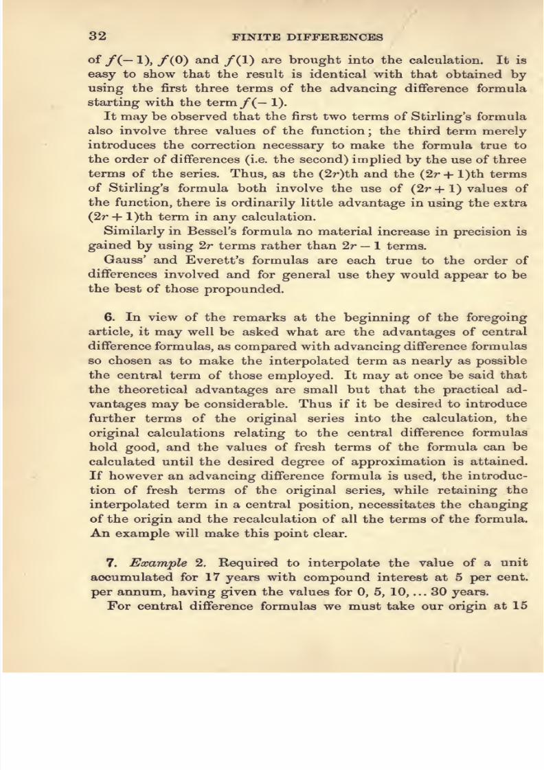
It may be observed that the first two terms of Stirling's formula
also involve three values of the function ; the third term merely
introduces the correction necessary to make the formula true to
the order of differences (i.e. the second) implied by the use of three
terms of the series. Thus, as the (2r)th and the (2r + l)th terms
of Stirling's formula both involve the use of (2r+l) values of
the function, there is ordinarily little advantage in using the extra
(27* + l)th term in any calculation.
Similarly in Bessel's formula no material increase in precision is
gained by using 2r terms rather than 2r — 1 terms.
Gauss' and Everett's formulas are each true to the order of
differences involved and for general use they would appear to be
the best of those propounded.
6. In view of the remarks at the beginning of the foregoing
article, it may well be asked what are the advantages of central
difference formulas, as compared with advancing difference formulas
80 chosen as to make the interpolated term as nearly as possible
the central term of those employed. It may at once be said that
the theoretical advantages are small but that the practical ad-
vantages may be considerable. Thusif it
bedesired to introduce
further terms of the original series into the calculation, the
original calculations relating to the central difference formulas
hold good, and the values of fresh terms of the formula can be
calculated until the desired degree of approximation is attained.
If however an advancing difference formula is used, the introduc-
tion of fresh terms of the original series, while retaining the
interpolated term in a central position, necessitates the changing
of the origin and the recalculation of all the terms of the formula.
An example will make this point clear.
7. Example 2. Required to interpolate the value of a unit
accumulated for 17 years with compound interest at 5 per cent,
per annum, having given the values for 0, 5, 10, ... 30 years.
For central difference formulas we must take our origin at 15

7/27/2019 7-CALCULUS AND PROBABILITY-1922-Alfred Henry.pdf
http://slidepdf.com/reader/full/7-calculus-and-probability-1922-alfred-henrypdf 47/170
CENTRAL DIFFERENCES 83
years, and we will take 5 years as the unit. Thus we get the
following scheme
No. of
yearsX /(^) A A2 A3 A* A5
-3 1- -27628 •07633 •02110 -00580 -00165
5 -2 1-27628 -35261 -09743 -02690 •00745 -00206
10 -1 1-62889 -45004 •12433 -03435 -00951
15 2-07893 -57437 -15868 •04386
20 1 2-65330 •73305 -20254
25 2 3-38635 -93559
30 3 4-32194
As the unit of time is 5 years, the required value is repre-
sented by/(*4).
Central Differences. We will use Gauss' formula, i.e.
/(«)=/(0)+ «;A/(0)
The successive terms, with the corresponding values of /(•4), are
/(O) =2-07893,
1stapprox. = 2-07893
•4A/(0)= •22975,2nd „ =2*30868
'^-^^^Ay(-1)=- •01492,3rd „ =2-29376
1-4 X -4 X - -6
^3y>(_i) ^ , .QQj^g2, 4th „ =2-29184
1-4 X -4 X - -6 X - 1-6
24Ay(-2)= •00017,5th
2-4xl4x4x--6x-l-6
120A»/(- 2)= -00002, 6th
= 2-29201
= 2-29203
It is clear that no further terms would affect the calculated
value. The true value is 2-29202.
H. T.B.I.

7/27/2019 7-CALCULUS AND PROBABILITY-1922-Alfred Henry.pdf
http://slidepdf.com/reader/full/7-calculus-and-probability-1922-alfred-henrypdf 48/170
84 FINITE DIFFERENCES
Advancing Differences.
1st approximation /(O) = 2-07893,
2nd approximation /(O) + '4A/(0) = 2*30868,
3rd approximation
/(- 1) + 1-4A/(- 1) + ^^^^ A^/(- 1) = 2-29376,
4th approximation
/(-l) + l-4A/(-l)+l^AV(-l)
+ ^ ^'''t'' ^ ^'/(-l) = 229184.
5th approximation
/(- 2) + 2-4A/(- 2)+ii^ AV(- 2)
H-?^^^H^A./(-2)
-H^ ^^^'V;''-'
Ay(- 2) = 2-29200.
6th approximation
. 2-4 X 1-4 Xn -A
120
/ci-i. • ^- \ 2-4xl-4x-4 x--6x-l-6 .. -. ^. « «^«^.^(6th approximation) + — A»/(- 2)= 2-29202.
Itwill be
observed that in proceeding to the 3rd and 5th ap-proximations using advancing differences every term in the formula
has to be recalculated, whereas, in the application of the central
difference formula, terms already calculated hold good whatever
be the degree of approximation.
It should be noted, however, that both formulas give mathe-
matically the same results, the difference of a unit in the final
figure being due to the use of only five places of decimals
throughout.
8. As regards other practical points, it may be observed that
the numerical coefficients in the central difference formulas are
smaller than those in the advancing difference formulas (see
Example 2).
Other advantages arise in special cases. Thus Bessel's formula

7/27/2019 7-CALCULUS AND PROBABILITY-1922-Alfred Henry.pdf
http://slidepdf.com/reader/full/7-calculus-and-probability-1922-alfred-henrypdf 49/170
CENTRAL DIFFERENCES 35
can conveniently be applied for the bisection of an interval, since
the alternate terms vanish, giving
/(i) ,/(0)+/(l) l A'/(-l)^A^/(0)
8
3 AV(~2) + Ay(~l)^128 2
^- ^^^•
Everett's formula gives the same value.
9. It should be noted as regards Everett's formula, that in cal-
culating a series of values the work is nearly halved since it will
be found that terms in the formula can be made to do duty twice,
a? terms reappearing in the calculation as y terms.
This will be seen at once, for,
/W = «;/( ) +a;(a^-l)
3-Ay(0) +
a (a '-l)(a^-4)
5Ay(-i)+...
+ym +^-^ Ay(_ 1)y^y'-y-^)
Ay(-2)
and
/(i+y)=y/(2)+y(y'-i)
3AV(1) +
5A'/(0) +
f^/(l) + ^^A^/(0)-.^(^^^f^^)Ay(-l)+....
the last line being identical with the first. Thus, if we are inserting
terms in a series by subdividing the interval into five equal parts,
X = '2, '4, ... and 3/= '8, '6, Therefore half of the terms used
in the calculation of/(•2) can be made to do duty in the calculation
of /(I '8), and similarly for the other terms.
10. An example will indicate the method of working.
Example 3. Using Everett's formula, interpolate the missing
terms in the following series, between /(40) and/(50).
X /(^) A A2 A^ A*
30 771 91 48 36 5
35 862 139 84 41 37
40 1001 223 125 78 28
45 1224 348 203 106
50 1572 551 309
55 2123 860
60 2983
3—2

7/27/2019 7-CALCULUS AND PROBABILITY-1922-Alfred Henry.pdf
http://slidepdf.com/reader/full/7-calculus-and-probability-1922-alfred-henrypdf 50/170
36 FINITE DIFFERENCES
The coefficients of the several terms in Everett's formula are
•2 - -032 -006336
•4 - -056 -010752
•6 - -064 -011648
•8 --048 -008064
The work may be arranged in tabular form:
X x/(l) ^<t%V(0)x{x^.l)(x^.A) Sum of first
three terms
(2) + (3) + (4)
Sum of
second
three
terms
Interpolated
result
(5) + (6)6
^^^ ^^
(1) (2) (3) (4) (5) (6) (7)
•2
•4
•6
•8
200-2
400-4
600-6
800-8
- 2-6
- 4-7
- 5-4
- 4-0
0-0
01*
0-1
0-0
197-6
395-8
595-3
796-8
•2
•4
•6
•8
244-8
489-6
734-4979-2
- 4-0
- 70
- 8-0- 6-0
0-2
0-4
0-40-3
241-0
483-0
726-8973-5
796-8
595-3
395-8197-6
1037-8
1078-3
1122-61171-1
•2
•4
•6
•8
314-4
628-8
943-2
1257-6
- 6-5
-11-4
-13-0
- 9-7
0-2
0-3
0-3
0-2
308-1
617-7
930-5
1248-1
973-5
726-8
483-0
241-0
1281-6
1344-5
1413-5
1489-1
Columns (2), (3) and (4), which represent the first three terms of
the formula, are obtained by ordinary multiplication. Column (5)
gives the sum of these terms. From what has been said above, it
is clear that column (6), which represents the second set of three
terms of the formula to fourth central differences, is obtained by
writing down, in reverse order, the values of column (5) applicable
to the previous group of terms. The addition of columns (5) and
(6) then gives the desired result.
Thegiven values of
f{w)have been taken from the tabulated
values of the probability of dying in a given year of age according
to the H^ mortality table, multiplied by 10^
The tabular values for the interpolated terms are 1038, 1081,
1122, 1172, 1281, 1345, 1415, 1490. The small differences between
these values and the interpolated values are due to the fact that
the H^ table was constructed by means of a mathematical formula
which is only approximately represented by Everett's formula.

7/27/2019 7-CALCULUS AND PROBABILITY-1922-Alfred Henry.pdf
http://slidepdf.com/reader/full/7-calculus-and-probability-1922-alfred-henrypdf 51/170
CENTRAL DIFFERENCES 37
11. Another method of applying the principles of central
differences is to express the required function in terms of known
values of the function among which it occupies a central position.
This can conveniently be done by Lagrange's formula. The for-
mulas are of two types according as the number of terms involved
is odd or even. Thus we have by Lagrange
Number of terms 2n + 1.
3-term formula,
fix)
^
/(-l) /(O) /(I)
xix'-l) 2(a;+l) X '^2(a;-l) ^^'
5-term formula,
/(-2) /(-I) /(O) /(I)J
'A(x+2) 6(a +l)'^ 4a; 6(a -l) ^24
.(7).
f(x) ^ /(-2) /(-I) /(O) /(I) /(2)
a;(a^-l){a^-4,) 24( c+2) 6(a;+l)^ 4a; 6(a -l) ^24(a;-2)
7-term formula,
fix) ^ /(-3) /(-2) /(-I)
a?(ic2- l)(ar^-4)(a^^-9) 720(a; + 3) 120 (a? -}-2) *
48 (a; + 1)
/(O) /(I) /(2) /(3)
36^ 48(a;--l) 120 (a; -2) ^720 (a? -3) ^^'
Number of terms 2n,
^-term formula,
/{«=) ^ /(-f) , /(-i) fih),
/(f)
(^_j)(«,._9) 6(a; + f) ^2(a;+ i) 2(a;-i)'^6(a;-f)
(9).
Q-term formula,
(a^-i)(a:2-|)(a;2_^) 120(a; + f) ^24(a; +f)
/(-t), /(4) /(f) , /(t) .10^
12ix + \)^12ix-\) 24 (a; -f) ^120 (a;- f)' ^ ^*
12. These formulas, of course, yield identically the same results
as other central difference formulas embracing the same terms.
To illustrate this we will recalculate the value of /(•4) in the
example given in § 7.

7/27/2019 7-CALCULUS AND PROBABILITY-1922-Alfred Henry.pdf
http://slidepdf.com/reader/full/7-calculus-and-probability-1922-alfred-henrypdf 52/170
38 FINITE DIFFERENCES
Example 4. See Example 2. Seven terms are given, the formula
will therefore be
/(I) ^ /(-3) f(-2)/(-I)
•4 (-16 - 1)(-16 - 4) (16 - 9) 720 x 3-4 120 x 24
^48 x 1-4
/(Q),
/(I) /(2) /(3) ^
36 X-4 ^ 48 X - -6 120 x - 1*6
^720 x - 26
or /(•4) = - •0046592/(- 3) + •0396032/(- 2) - •169728/(- 1)
+ -792064/(0) + -396032/(1) - -0594048/(2) + -0060928/(3)
= + -05055 - -00466
1-64665 -27647
1-05079 -20117
-02633
+ 2-77432 -48230
= 2-29202 as before.
Note, as a check, that the algebraic sum of the coefficients of the
terms on the right-hand side of the above equation is unity.
13. For the sake of completeness it is necessary to refer to a
system of notation in connection with central dififerences which
was introduced by W. S. B. Woolhouse and is still in use to some
extent. This system of notation is compared with that used in the
previous chapters in the following scheme
Ordinary Notation Woolhous^s Notation
/(-2) /(-2)A/(-2) a_2
/(-I) Ay(-2) /(-I) &-1A/(-l) a3/(-2) a_i c_i
/(O) A2/(-l) Ay(-2) /(O) (oo) bo (Co) do
A/(0) A3/(-l) « Ci
/(I) Ay(0) /(I) b,
A/(l) Oj
/(2) /(2)
where A/(- 2), A'*/(- 2), etc. are denoted by a_2, &-i, etc. andtto = J (a_i + a+i)>
Co = J (c-i + c+i).
Under this notation Stirling's formula to fourth differences is
/W =/(0) + ^ao +2j^0+3 ^0 +
41^o
=/(0)+(ao.g).+(2VJ;)^
+ |^,^4-|^ ...(11).

7/27/2019 7-CALCULUS AND PROBABILITY-1922-Alfred Henry.pdf
http://slidepdf.com/reader/full/7-calculus-and-probability-1922-alfred-henrypdf 53/170
CENTRAL DIFFERENCES 39
Similarly Gauss' formula can be written
^(.+ l).fa-l)(.-2)^^^^2).
t
14. Another system of notation, which is extensively used, is
that due to W. F. Sheppard. Two operators B and fi are used, such
that
S/(- i) =/(0) -/(- 1), /»/(*) = i [/(O) +/( )],
2/(i) =/(l) - /(O), m8/(0) = i [S/a) + 8/(- i)],
etc. etc.
This notation, although somewjiat complicated, gives the usual
central difference formulas in very convenient forms.
7/27/2019 7-CALCULUS AND PROBABILITY-1922-Alfred Henry.pdf
http://slidepdf.com/reader/full/7-calculus-and-probability-1922-alfred-henrypdf 54/170
CHAPTER VIFINITE DIFFERENCES. INVERSE INTERPOLATION
1. In direct interpolation a series of values of the function is
given and the problem is to find the value of the function corre-
sponding to some intermediate value of the argument.
In Inverse Interpolation the problem is reversed and it is required
tofind
the valueof
the argument which corresponds to some valueof the function, intermediate between two tabulated values.
2. In certain cases of mathematical functions the desired result
can be obtained by direct calculation. Thus if
log a'
and the value of x can be found equivalent to any given value
ofy.
Where this is not the case various methods can be adopted.
These will be examined in order.
3. Let y =f(x) be the given value. Then
y =/(^) =/(0) + ^A/(0) +?^^ A»/(0) + ....
If it be assumed that the higher orders of differences vanish, and
that the values of A, A^, etc. are obtained from the given terms of
the series, then we have an equation in os which can be solved by
the usual methods.
The disadvantages of this plan are firstly that an equation of
higher degree than the second is troublesome to solve, and secondly
that for certain functions the degree of approximation may not
be very close. Since a quadratic equation employs only three terms
of the series, it often happens that no close approximation can be
obtained. In all cases the intervals between terms should be as
narrow as possible, so that accuracy may be increased and the use
of higher orders of differences obviated as far as possible.

7/27/2019 7-CALCULUS AND PROBABILITY-1922-Alfred Henry.pdf
http://slidepdf.com/reader/full/7-calculus-and-probability-1922-alfred-henrypdf 55/170
INYERSE INTERPOLATION 41
4. This difficulty of solving an equation in x of higher degree
than the second can be overcome in two ways. Assume, for purposes
of illustration, that four values of the function are given, viz./(0),
/(l),/(2)and/(3).
Then
/W =/(0) + ^A/(0) +?^^> A»/(0) +^(^-^'^-2) ^a/(o).
No further differences can be calculated and therefore, since f(x)
is known, the corresponding value of x is found by the solution of
a cubic equation in x. The solution of the cubic can however be
avoided by proceeding as follows
Taking three terms only at a time
/W =/(0) + xAf(0)+ ^^^ AV(0).
and f(x) =/( ) + («- 1) A/(l) +(^-^K^-^)
A'fa).
The third difference error in the first equation is
( -y -'>A'/(o),
and, in the second equation.
If now both sides of these equations be multiplied respectively by
(3 — x') and x (where x is a rough approximation to the required
value, obtained by inspection) and the equations so weighted be
added together, a new quadratic equation in x will be formed from
which the third difference error will be practically eliminated. The
work of solving a cubic equation has been avoided, but all terms
have been used without sensible loss in accuracy.
If the mere arithmetic mean of the equations were taken, with-
out weighting as above, it is possible that, in certain cases, a worse
result would be obtained by taking four terms instead of three.
5. Alternatively the solution of the equation may be obtained
by successive degrees of approximation.
Thus, taking the above equation and neglecting differences of
the second and higher orders, we obtain as a first approximation
the value a? , where
^ m-m (1).
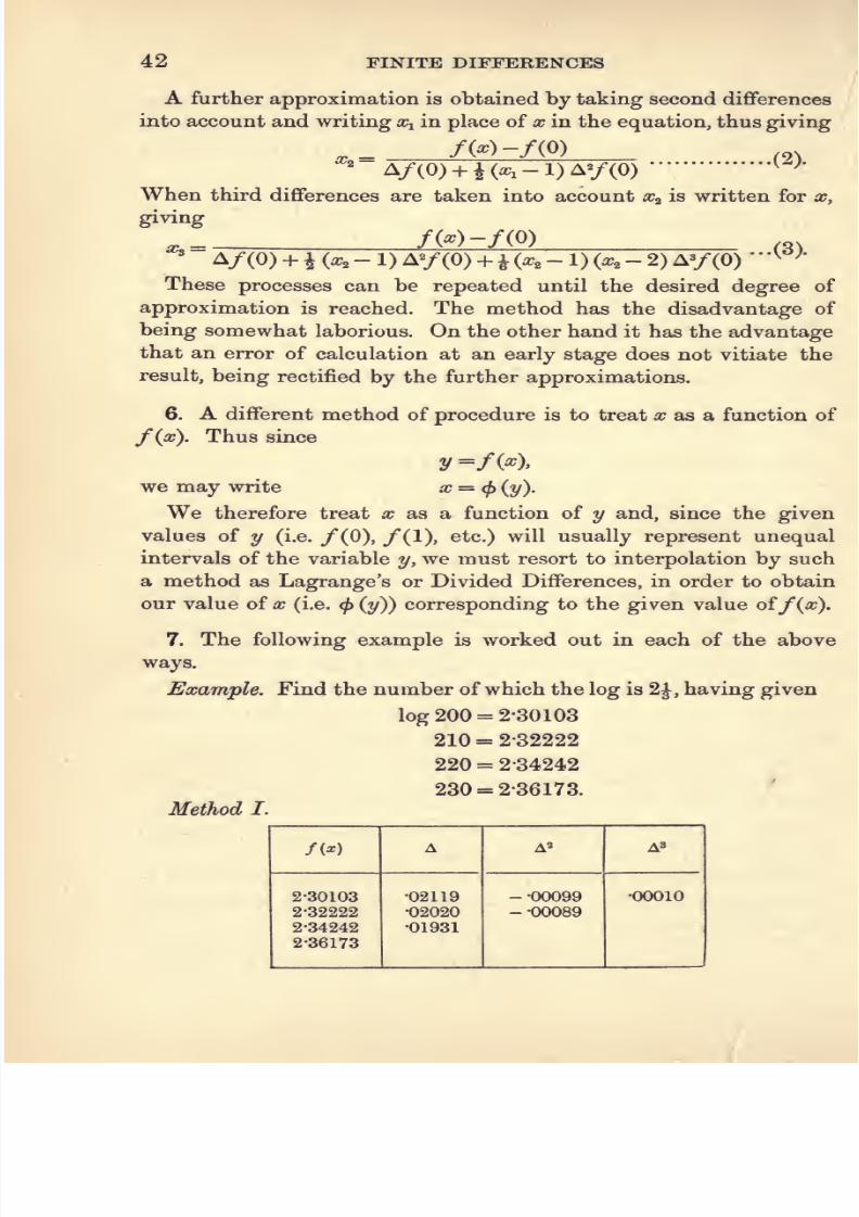
7/27/2019 7-CALCULUS AND PROBABILITY-1922-Alfred Henry.pdf
http://slidepdf.com/reader/full/7-calculus-and-probability-1922-alfred-henrypdf 56/170
42 FINITE DIFFERENCES
A further approximation is obtained by taking second differences
into account and writing x^ in place of x in the equation, thus giving
/W-/(0)Xn (2).A/(0) + H^i-l)Ay(0)
When third differences are taken into account x^ is written for x,
giving
/W-/(0)0 ,= ...(3).
V(0) + i («^ - 1) AV(0) + K^s - 1) (^ - 2) Ay(0)
These processes can be repeated until the desired degree of
approximation is reached. The method has the disadvantage of
being somewhat laborious. On the other hand it has the advantage
that an error of calculation at an early stage does not vitiate the
result, being rectified by the further approximations.
6. A different method of procedure is to treat a; as a function of
f(x). Thus since
y =/W»
we may write x = <l> (y).
We therefore treat x as a function of y and, since the given
values of y (i.e. /(O), /(I), etc.) will usually represent unequal
intervals of the variable y, we must resort to interpolation by such
a method as Lagrange's or Divided Differences, in order to obtain
our value of x (i.e. <^ (y)) corresponding to the given value of/(a?).
7. The following example is worked out in each of the aboveways.
Example, Find the number of which the log is 2J, having given
log 200 = 2-30103
210=2-32222
220 = 2-34242
230 = 2-36173.
Method I.
fix) A A2 A3
2-30103
2-32222
2-34242
2-36173
-02119
•02020
•01931
-•00099
- -00089
•00010

7/27/2019 7-CALCULUS AND PROBABILITY-1922-Alfred Henry.pdf
http://slidepdf.com/reader/full/7-calculus-and-probability-1922-alfred-henrypdf 57/170
INVERSE INTERPOLATION 43
f{x) = 2-33333 = 2-30103 + -02119^ - -00099 ^i^ll^
+-oooio-(--^>^--^\
b
Or, by reduction,
a^ - 32-7a;« + 1303-la? - 1938 = 0.
Whence, solving the cubic,
^ = 1-5443.
Since the initial value of x is 200 and the unit of measurement
is 10, the result of the calculation is to give 215-443 as the required
value of X.
8. Method II.
f(x) = 2-30103 + -021190; - 00099 ^i^Ili^
also, f(x) = 2-32222 + -02020 (x-1)- -00089 (^-^K^ ^).
The first approximation to the value of x is x' = l'5, so that
3 — a?' = 1-5. Since the values of S—x and x^ are approximately-
equal, we may take for our weighted equation the arithmetic
mean of the above equations, giving
/(a?) = 2-33333 = 2-30108 + -02161a;- -00047 o?^
Whence, solving the quadratic, a; = 1-5443 as before.
9. Method III.
1st approximation
2-33333-2-30103 , .^,„^^=^02119
=^* ^^'^»
2nd approximation
2 33333 - 2-30103
^^ •02119 -i X -5243 x-00099 ^*^'*'^'^'
3rd approximation
^ 2-33333 - 2-30103
^' -02119 - I X -5432 x -00099 + J x -5432 x (-5432 - 1) x -00010
= 1-5442,
which differs only slightly from the value obtained by Methods I
and II.

7/27/2019 7-CALCULUS AND PROBABILITY-1922-Alfred Henry.pdf
http://slidepdf.com/reader/full/7-calculus-and-probability-1922-alfred-henrypdf 58/170
44 FINITE DIFFERENCES
10. Method IV. Under this method we may consider the data
to be as follows
X fix)
2-30103
2-32222
2-34242
2-36173
200
210
220
230
It is required to find the value of/(2-33333). By Lagrange,
^.g.oqqoqx _ ('OHH) (^ 00909) (- '02840)
/ (2 SSSSS) - ^_ .^2119) (- -04139) (- '06070) ^^^
C03230)(- -00909) (--02840) ^
(-02119) (- -02020) (- 03951)
(-03230) (-01111) (--02840)
(-04139) (-02020) (- 01931)
(03230) (01111) (-00909)^
(06070) (-03951) (01931)
= - 10-7748 + 103-5416 + 138-8764 - 16-2006
= 215-443.
This result agrees with the values previously found. The true
value is 215-442 and it will be seen, therefore, that all of these
methods give results in this case which are closely approximate to
the true value.
11. Methods I—III differ from Method IV, in that the first
three methods assume that/(ic) is a parabolic function of x, whereas
Method IV assumes that x can be expressed as a parabolic function
oi f{x). Both these assumptions may be sufficiently accurate in
many cases, but in other cases an inspection of the trend of the
given values of the function may indicate which assumption is to
be preferred.
12. By the use of the formulas of Divided Differences given in
Chapter VIII, Methods I—III can be applied to cases where the
given values of the function are at unequal intervals.
The application of Method IV is, of course, perfectly general.

7/27/2019 7-CALCULUS AND PROBABILITY-1922-Alfred Henry.pdf
http://slidepdf.com/reader/full/7-calculus-and-probability-1922-alfred-henrypdf 59/170
CHAPTEK VII
FINITE DIFFERENCES. SUMMATION OR INTEGRATION
1. Summation is the process of finding the sum of any number
of terms of a given series. This can be accomplished either if the
law of the series is known or if a sufficient number of terms is given
to enable the law to be ascertained. As will be shown in Chapter XX,
if no mathematical law is apparent, methods can be applied bywhich the approximate sum of a series can be obtained.
2. Consider a function F{x) whose 1st difference is f{x). Then
we have
^(1) -^(0) =/(0)
Fit) -F(V, =/(l)
F{a) -F(a-l)=f(a-l)
F(a+ 1)-F(a) =f(a)
F{n-l)~F{n-2)=f(n-2)
F(n) -F(n-l)=fin-l).
Summing both sides, we obtain
J'(n)-^(0)=/(0)+/(l) +...+/(„- )
or F{a)-F(0)=f(0)+f(l) +...+/(<»- 1)
or F(n)-F(a)=f(a)+/(a + l)+...+f(n-l) ...(1).
It is clear, therefore, that the sum of any number of terms of a
series of values oif{x) can be represented by the difference between
two values of another function F (x) whose 1st difference is /(a;).
By analogy with the system of notation already adopted for ex-
pressing orders of differences, the process of finding the function
whose 1st difference is f{x) may be denoted by A~^ /(a?). It is
n-l
customary to express /(O) +/(1) + ... +/(w — 1) as 2 /(a?), the
terms at which the summation is commenced and terminated
(designated respectively the inferior and superior limits of sum-
mation) being indicated m tb^ manner shown.

7/27/2019 7-CALCULUS AND PROBABILITY-1922-Alfred Henry.pdf
http://slidepdf.com/reader/full/7-calculus-and-probability-1922-alfred-henrypdf 60/170
46 FINITE DIFFERENCES
3. The process of finding the value of F{x) is known as Finite
Integration and F (x) is called the Finite Integral of f(x). Where
the limits of summation are known we obtain by summation of
f{x) the Definite Integral of /(a;); if the limits of summation are
not expressed we obtain merely the Indefinite Integral oif(x).
4. As stated above, in obtaining the indefinite integral of f(x)
no point is specified at which the summation is to commence and,
since an unknown number of terms of the series is included, it is
necessary to include in the value of F(x) a constant term which is
of unknown value.
This constant vanishes in the case of definite integrals, since if
Xf{x) = F(x) + c,
then X fix) = [F (n) -{-c]-[F (0) + c]
= F(n)-F(0).
5. It is obviously always possible to find the first difference of
any function, but it does not follow that every function can be
integrated. The functions which can be integrated are limited in
number and the process of integration rests largely on the ingenuity
of the solver aided by such analogous forms as may be obtained by
the formulas of finite differences.
Thus we have A a* = (a - 1) a*
whence it is easily seen that
a — 1
and therefore, since the result of differencing is to give a*,
we have
a — I
where c is the constant introduced by integration.
The sum of the series a* + a^+^ 4- ... + a* ^^^ is at once obtained
r+n-l
by finding the value of the definite integral 2 a*, which by § 2r
,r+na'
is equal to r- r- , which agrees with the familiar result for
the sum of a geometrical progression.
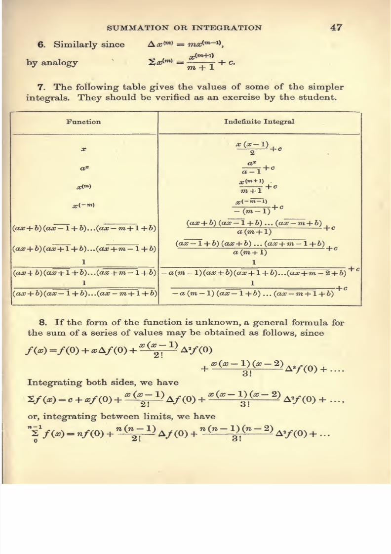
7/27/2019 7-CALCULUS AND PROBABILITY-1922-Alfred Henry.pdf
http://slidepdf.com/reader/full/7-calculus-and-probability-1922-alfred-henrypdf 61/170
SUMMATION OR INTEGRATION
6. Similarly since Aa;<^) = inx^'^^\
by analogy
47
m + 1
7. The following table gives the values of some of the simpler
integrals. They should be verified as an exercise by the student.
Fanotion Indefinite Integral
a;{x—l)
a;(- »)
2
a
a-l
^(m + l)
Wl+ l
-{m-1)
+c
+c
+c
+ c
{cuc+h){ax-l-\'b)...(aa;-m+l+b){ax-\-h) {ax—\ + h) ... {ax-m-\-h)
a (m+ 1)+ c
(cM7+6)(aa7-fl+6)...(a^+w-l + 6)
1
{(ix-l-^h){ax-\-h) ...{ax+m-\ + h)
a (m+1)
1
+c
(flw;+6)(flM7+l+6)...(a^+m-l-f6)
1
(flW7 4- ^) (cm; - 1 + 6). . .(a^ - m+ 1 + 6)
a{m-\){ax+ h){ax-\-l-\-h)...{oLx-\-m-'2.+ b)
1
-+c
+c
a(m-l)(a^-l + 6)...(aa7-m + l4-6)
8. If the form of the function is unknown, a general formula for
the sum of a series of values may be obtained as follows, since
fix) =f(0)+ xAf(0)+ ^^^ A«/(0)
Integrating both sides, we have
or, integrating between limits, we have
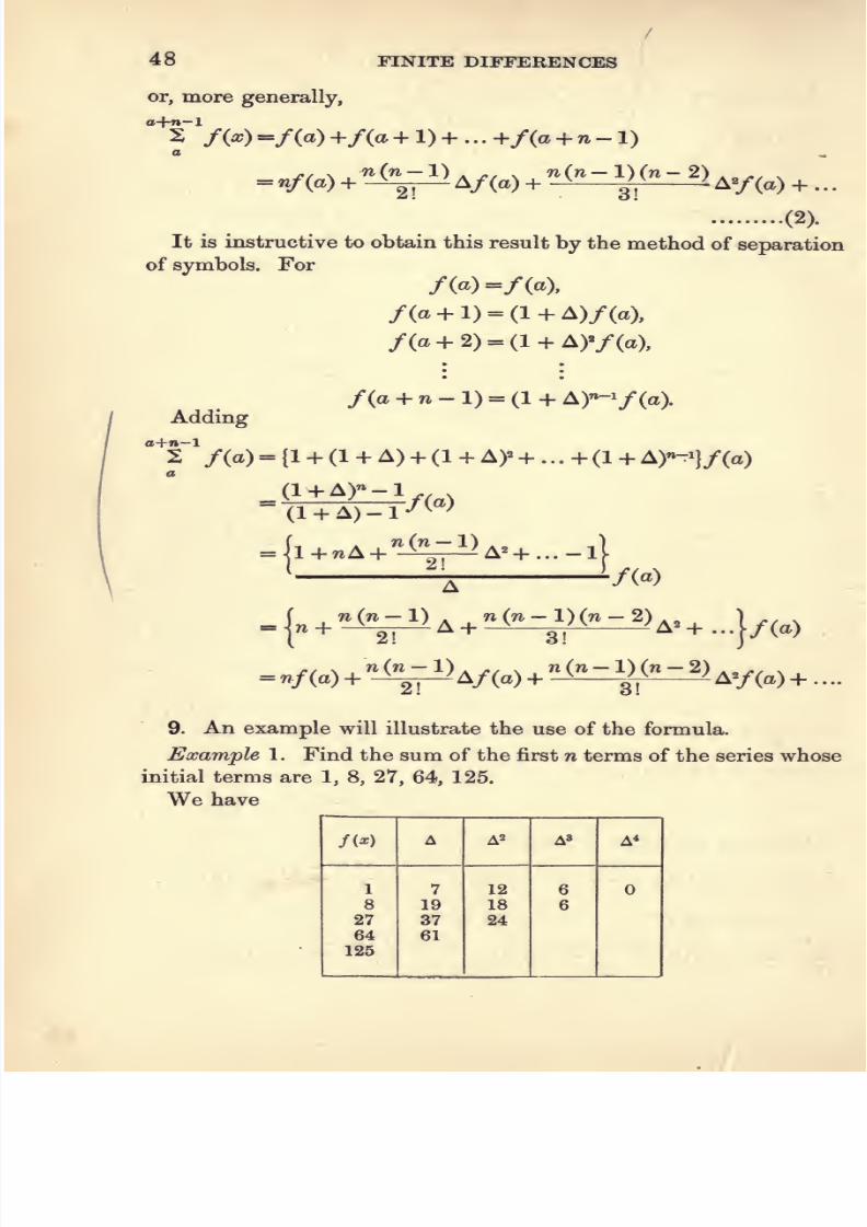
7/27/2019 7-CALCULUS AND PROBABILITY-1922-Alfred Henry.pdf
http://slidepdf.com/reader/full/7-calculus-and-probability-1922-alfred-henrypdf 62/170
48
or, more generally,
a+n-l
FINITE DIFFERENCES
.,. -71(71-1) .-, . W(^— 1)(^-- 2) ^„ ., ^
= nf((^) + -^^2— ^^( ^^ ^ ^
3^y( *) + • •
•
(2).
It is instructive to obtain this result by the method of separation
of symbols. For
/(o + l) = (l + A)/(a),
/(a+2) = (l + A)'/(a),
Adding
/(a + n-l) = (l + A)'-/(o>
o+n-l
2 /(a) = {l + (H-A) + (l+A>'+...+(l+A)'->)/(o)
(1 + A)»-1., ,
=(l + A)-l
-^( >
*
^A ^/W
=.{.-H--(^A^ (-3V( -^>
A'-H }/(.)
= «/(a) + ^>A/(a) + -^\(^^ A'/(a)+ ....
9. An example will illustrate the use of the formula.
Example 1. Find the sum of the first n terms of the series whose
initial terms are 1, 8, 27, 64, 125.
We have
/(^) A A2 A3 A«
1 7 12 6
8 19 18 6
27 37 24
64 61
125

7/27/2019 7-CALCULUS AND PROBABILITY-1922-Alfred Henry.pdf
http://slidepdf.com/reader/full/7-calculus-and-probability-1922-alfred-henrypdf 63/170
SUMMATION OR INTEGRATION 49
Whence
v^^^z X 1.w(n~l) ^ n(n-l)(n-2) ^^
S f{x) = nxl+ ^^^
^ x7+— ^p ^xl2n-l
n(7i-l)(n-2)(n~3)^^g
4~
4
which agrees with the formula for the sum of the cubes of the
natural numbers.
10. Where it is desired to integrate a function which is the
product of two factors, the following device may often be utilised
with advantage.
Let the function be y = UxVg^
Then Au^v^= u^+iV^+i - u^Va^
= Ux+i (Vx+i - Vx) + Vx {Ux+i - Ux)
Integrating both sides of the equation, we obtain
or '2,VxAUx = UxVx-'^Ux+iAVa: (3).
Thus, if the original function can be put in the form Vx^Ua;, its
integral can be made to depend upon that of Ux+i^Vx, and, if the
latter is in a form which can be readily integrated, the value of anapparently intractable integral may often be obtained in this way.
Example 2. To find the value of Xxa^.
qX
Since Sa* = r , we may write
2a?a* = I.Xa-1'
Using the above formula (3) we
^ Aa^ xd^Zx -=
z.
a—1 a—
get
Ax
xa'^
~a-l a-1, since Ax =
= 1,
ica* a^+^+ c.
a-1 (a-iy
H. T. B. I.

7/27/2019 7-CALCULUS AND PROBABILITY-1922-Alfred Henry.pdf
http://slidepdf.com/reader/full/7-calculus-and-probability-1922-alfred-henrypdf 64/170
50 FINITE DIFFERENCES
11. Sometimes it may be necessary to apply the formula more
than once in order to reduce the integral by stages to a standard
form. The process is illustrated in the following example.
Example 3. To find the value of 22^a:^.
Remembering that A2^ = 2*^, we may write
= a,'32'^-22*+iAa^
= 3^2^^ ^ 22^+1 (3ic2 + 3^ ^ 1)^
It will be observed that in applying formula (3), the degree of
X, in the terms within the integral, has been reduced by unity.
Proceeding as before we obtain
22 '^^ = a;32x _ 2: (3^ + 3a; + 1) A2*+i
= a,''2^ - [2=^+1 {^a? + 3^ + 1) - 22=^+2A (3a;« + 3a; +1)]
= 2=^ (a;» - 6a;=^ - 6a; - 2) + 22=^+2 (g^ _,. g)
= 2^^ (a;^ - 6a;2 - 6a; - 2) + 2 (6a; + 6) A2^+2
= 2* (a;» - ear - 6a; -2) +
[2^^+^ (6a;
+ 6)
- S2=«+»
A(6a;
+ 6)]
= 2* (a? - 6a;« + 18a; + 22) - 22*+* X 6
= 2^(a;»-6ar^4-18a; + 22)-6x2^+' + c
= 2=^(a;3 _ g^^ 18a;- 26) + c
The above process is analogous to that of Integration by Parts,
which is dealt with in the Integral Calculus, Chapter XVIII, § 6.

7/27/2019 7-CALCULUS AND PROBABILITY-1922-Alfred Henry.pdf
http://slidepdf.com/reader/full/7-calculus-and-probability-1922-alfred-henrypdf 65/170
CHAPTER VIII
FINITE DIFFERENCES. DIVIDED DIFFERENCES
1. A simple method of interpolation is available, where the in-
tervals between the given terms are unequal, by the method of
Divided Differences.
2. The application of the method rests upon the assumption,
which, as has been shown, is the basis of all theorems for interpola-
tion by means of Finite Differences, that f(oc) is a rational integral
function of oo of the nth. degree.
On this assumption, it can be shown that f(os) can be expressed
in the form
^0+ ^1 (^ - ^i) + ^2 (^ - ai)(^ — ^a) + . .
+ An{oo- aO (a? - ttg) . . . (a? - an),
where Aq, Ay, ... An, Oi, ag, ... «« are constants.
3. In order to apply this formula in practice, it is convenient to
introduce a scheme of notation on the following lines, where the
symbol of operation is denoted by A' in order to distinguish it from
the ordinary A.
Value of XValue of
FunctionA' A'a A'3
02
03
/(O)
/(«2)
/(«4)
/(«,)-/(0)
/(«2)-/(ai)
a2-ai'
/(«3)-/(«2)
f{a,)-f{a,)
A'/(ai)-A7(0)
^2
A'f{a2)-A'f(a^)
A'f{a,)-A'f{<H)
a^-a2
A'7(ai)-A'V(0)
as
A'7(a2)-A'7(ai)
etc.
Generally, we have
Un+r-ar
4—2

7/27/2019 7-CALCULUS AND PROBABILITY-1922-Alfred Henry.pdf
http://slidepdf.com/reader/full/7-calculus-and-probability-1922-alfred-henrypdf 66/170
52 FINITE DIFFERENCES
Hence /(aO=/(0) + a,Ay(0),
and /(oa) =/(ai) + ((h-(h) A'/(ai)
=/(0) + a, A'/(0) + {a, - a,) {A7(0) + a, A'^f (0)}
=/(0) + a,A7(0) + a, (a, - a,) A'V(0).
By proceeding similarly for further terms, we find that we can
write generally
/W =/(0) + «^A7(0) + x(x-aO AV(0)
+ x(x-a,)(x- a,) A'7(0) + . . . (1).
This general form can be readily established by the method of
induction.
By giving appropriate values to ttj, Og, ... the ordinary formulas
applicable to equal intervals can be at once deduced.
4. The genera] method of working will be shown more simply
by an example.
Example. Find the value of log 4-0180, having given the fol-
lowing data:
Number Logarithm
4-0000
4-0127
4-0233
4-0298
4-0369
-6020600
•6034367
•6045824
-6052835
•6060480
Transposing the origin, we have the following scheme:
X /(^) A' A'2
0-0000 •6020600 •T.r=—- ^000317
•0233•0136
0-0127 -6034367 jr—- ^000223
-0171•0130
0-0233 -6045824 Ta ----- -000186
•0136•0137
0-0298 •6052835 ^-^-—0-0369 •6060480

7/27/2019 7-CALCULUS AND PROBABILITY-1922-Alfred Henry.pdf
http://slidepdf.com/reader/full/7-calculus-and-probability-1922-alfred-henrypdf 67/170
DIVIDED DIFFERENCES 53
We have to j&nd/('0180), which is, by the above formula,
/(O) + •0180A7(0) + -0180 X -0053AV(0)
[the further terms will not affect the seventh place of decimals],
where /(O) = '6020600, A7(0) = -108402, AV(0) = - '0136.
Thus log 4-0180 = -6020600 + -00195124 - 00000130 = -6040099
to seven decimal places, which agrees exactly with the true result.

7/27/2019 7-CALCULUS AND PROBABILITY-1922-Alfred Henry.pdf
http://slidepdf.com/reader/full/7-calculus-and-probability-1922-alfred-henrypdf 68/170
CHAPTEE IX
FINITE DIFFERENCES. FUNCTIONS OF TWO VARIABLES
1. Questions involving functions oftwo variables arise frequently
in actuarial practice. Thus the tabulated values of functions (e.g.
annuities) dependent upon two lives may be given only for com-
binations of quinquennial ages in order to economise space. If the
value corresponding to any other combination of ages is required,resort must be had to methods of interpolation.
2. In considering the problem of the changes induced in the
value of/(a;, y) by finite changes in the values of x and y we must
consider x and y as being independent of each other. Clearly, if
y were a function of x the expression f{x, y) could be made to
assume the form of a function of x alone and it could be dealt
with by the methods already developed in previous chapters.
Thus X may vary while y remains constant, so that, if x changes
to a;+ ^, the value of the function becomes f{x -|- ^, y); or y can
vary while x remains constant, giving a value fixyy-k-k)) or both
X and y can vary independently, giving a value for the function of
/{x^-h.y + k).
3. We shall proceed first to discuss the problem where the
values of the function are given for combinations of successive
equidistant values of x and y.
Thus we may have
f{^> y) /(^ + ^> y) /(^ + 2A,, t/) ... f{x 4- mh, y)
f(x,y + k) f(x + h,y + k) f(x-\-2h,y-^k) ,..f(x+mh,y + k)
f(x,y + nk) f{x+h,y+nk) f{x-\-2h,y+ nk) ...f{x-\-mh,y+nk)
As has already been seen in the case of functions of one variable
(Chapter III, § 6), this scheme can be simplified, for the origin can
be placed at the point {x, y), and the unit of measurement can be
taken as h in the case of the variable x and k in the case of the
variable y.
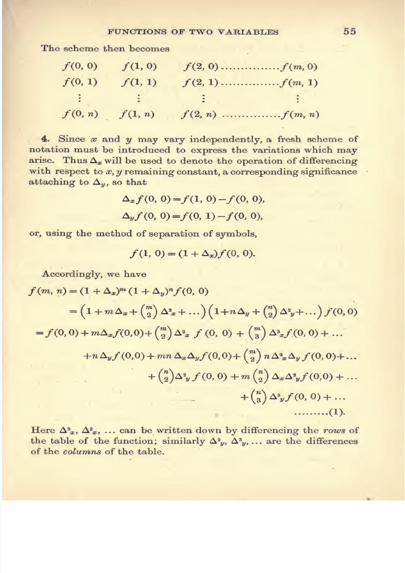
7/27/2019 7-CALCULUS AND PROBABILITY-1922-Alfred Henry.pdf
http://slidepdf.com/reader/full/7-calculus-and-probability-1922-alfred-henrypdf 69/170
FUNCTIONS OF TWO VARIABLES 55
The scheme then becomes
/(0,0) /(1,0) /(2,0) /(m,0)
/(0,1) /(1,1) /(2,1) /(m,l)
/(0,n) /(1, 71) /(2,ri) /(m,n)
4. Since x and y may vary independently, a fresh scheme of
notation must be introduced to express the variations which mayarise. Thus A^. will be used to denote the operation of differencing
with respect to x, y remaining constant, a corresponding significance
attaching to Aj,, so that
A./(0,0)=/(l,0)-/(0,0),
^/(0.0)=/(0,l)-/(0,0),
or, using the method of separation of symbols,
/(l,0) = (l + A,)/(0,0).
Accordingly, we have
/(m, n) = (1 + A^r (1 + Ay)»/(0, 0)
=/(0,0) + mA,/(0,0)+(2)A», /(O, 0) + (3)A»,/(0,0)+ ...
+n^yf{0,0) + mn^^^yf{0,(i)+{^)n^^\f{Q,(i)+...
+ (2^/(0. 0)+mg)A,AV/(0,0) +...
+ (3)^^/(0.0)+-
(1)-
Here ^\, A^a,, ... can be written down by differencing the rows of
the table of the function; similarly A^^, A'y, ... are the differences
of the columns of the table.

7/27/2019 7-CALCULUS AND PROBABILITY-1922-Alfred Henry.pdf
http://slidepdf.com/reader/full/7-calculus-and-probability-1922-alfred-henrypdf 70/170
56 FINITE DIFFERENCES
To find Aj;A„, A'a,Ay, etc. we have
A,A,/(0, 0)= A, [/(O, l)-/(0, 0)]
=/(l. l)-/(0, 1)-/(1, 0)+/(0. 0).
A««A,/(0, 0) = A»,[/(0, 1) -/(O, 0)]
=/(2, 1) - 2/(1, 1) +/(0, 1) -f(% 0)
+ 2/(l,0)-/(0,0),
and so on.
Example 1. Table XVI of the Short Collection of Actuarial
Tables. To find -4 31:63, having given
•^3J:6o = -11669, A^,^ = -13190, ^4j,eo = -15494,
^30:66 = -09809, .^35,85= -11039,
^3J:70 = -07812.
Here m = i, w = J,and
A^= -01521, A*a,= -00783, Aa;Ay = - 00291,
Aj/ = - -01860, A^^y = - -00137.
Whence A^^,^ = -10776, the correct value being -10773.
5. An obvious method ofprocedure involving only first differences
is as follows. Obtain the value of/(O, n) by interpolation between
the values of /(O, 0) and /(O, 1). Similarly, obtain the value of
/(I, n) from the values of/(I, 0) and /(1, 1). Finally find/(m, n)
by interpolation between /(O, n) and /(I, n). Thus
/(O, n) = r=^/(0, 0) + 7?/(0, 1),
/(I, n)=l-rz/(l,0) + 71/(1,1),
/(r?i, w) = l-m/(0, n) + wi/(l, n)
=/(0, 0) + m A^/(0, 0) + n^yf (0, 0) + mnA ^ Aj,/(0, 0)
(2)
= 1 - m 1 - n/(0, 0) + 71 . 1 - m/ (0, 1)
+ m. 1^/(1, 0) + mn/(l, 1) ...(3).
Employing this formula in the example given above we find
^^63 = -10822.
The method is suitable if only a rough approximation is required,
but cannot be depended upon to give an accuratevalue.

7/27/2019 7-CALCULUS AND PROBABILITY-1922-Alfred Henry.pdf
http://slidepdf.com/reader/full/7-calculus-and-probability-1922-alfred-henrypdf 71/170
FUNCTIONS OF TWO VARIABLES 57
6. Obviously the method can be extended by taking higher
orders of differences. The disadvantage of this procedure is that
it involves the calculation of further values of the function corre-
sponding to a given value of a; as a preliminary to applying the
interpolation formula to find the value off(x,y). The process
thus becomes laborious and moreover we do not necessarily obtain
identical values for f(x, y) if we interpolate first with regard to x
and then with regard to i/, or vice versa.
7. As in the case of functions of one variable, we shall expect to
obtain the best results when the principles of central differences
are applied, i.e. when the required term occupies as nearly as pos-
sible a central position among the terms employed in the formula.
The difficulty is that, in dealing with functions of two variables,
we cannot adapt our formulas to any system of values which may
be given. Thus an inspection of the advancing difference formula
(1) shows that it involves points whose coordinates form a triangu-
lar plan which may be illustrated thus:
(0, 2)
o
(0, 1) (1, 1)o o
(0, 0) (1, 0) (2, 0)o o o
This illustrates the formula where two orders of differences are
taken into account, the black dot representing the interpolated
term. It will be seen that the scheme is hardly satisfactory from
the point of view of central differences. For most practical pur-
poses, however, where ordinary actuarial functions are involved,
formula (1) will give satisfactory results.
8. Formulas embodying the principles of central differences can
conveniently be obtained by an adaptation of Lagrange's for-
mula. This formula applied to functions of two variables has not
the same wide application as the ordinary formula of Lagrange
previously given in Chapter IV, but, as will be seen below, it gives
expressions for /(a;, y) in terms of the neighbouring values.

7/27/2019 7-CALCULUS AND PROBABILITY-1922-Alfred Henry.pdf
http://slidepdf.com/reader/full/7-calculus-and-probability-1922-alfred-henrypdf 72/170
58 FINITE DIFFERENCES
9. Generalformulafor 4i points.
Taking all combinations of two terms except those which give
rise to a^ and y , let
f(w,y) = A(x-^)iy-b) + B(x-^)(y-a) + Cix-a){y-a)
+ D(x-a)(y-b),
then /(a, a) = A(a-fi)(a- b),
f(a,b) = B(a-ff)(b-a),
/(/3,a) = 2)(/3-a)(a-6),
f(0,b) = O(0-a)ib-a),
whence, substituting for A, B, G and D in the original formula,
fix, y) ^f(«, a)(„_^)(„_6)+/(«,6)(„_^)(6-a)
(x-a)(y-a) . (x-a)(y-b)
10. General formula for 6 points.
Taking all combinations of two terms, let
f(x,y)==A(x-ff)(y^b) + B(x-^){y-a)+G(x-a)(y--a)
+ D(x-a)(y-b)-^E(x-a)(x--^)-\-F(y-a)(y-b).
Taking the points a : a, a :b, a : c, ff : a, ^ :b and 7 : a, and pro-
ceeding as before, we arrive at the result
f/. ,A - f(« «^ {(^-^)(y-J>)
,
(^-Ci)(x-0) (y-a){y-b) )
J ('«'. y) -/(«• a)1^^ _ „) (J _ „)
+(^ _ „) ^^
_ „)+
(6 _ a)(c - a)\
•^ ^ ' ^l(/3
- a)(6 - a) + (6 - a)(c - 6)|
, ^,„ . (y- )(y-<')
/rfl «^ ((' - Xy-fc)
,
(x-a)(x-0))
-J ^^' ^\{0 - «)(6 _ a) + (yS - a) (7 - ^)|
. ^.o i,^('^-«)(y-a)
.(5).

7/27/2019 7-CALCULUS AND PROBABILITY-1922-Alfred Henry.pdf
http://slidepdf.com/reader/full/7-calculus-and-probability-1922-alfred-henrypdf 73/170
FUNCTIONS OF TWO VARIABLES 59
11. Generalformula for ^ points.
Taking all combinations of two terms, each involving x, with
two terms each involving y, let
f{x,y)^A{x-P){x^y){y-h){y-c)
\-B(x-^)(x'-y)(y-a)(y-c) + G(x-/3)(x-y)(y-a)(y-b)
+ D(x-OL)(x^y)(y'-b)(y-c)-{-E(x-a)(x-y)(y-a)(y-c)
\-F(x~a)(x-y)(y-a)(y-h) + G(x-a)(x^j3)(y-h)(y-c)
+ ff(a)-a){x-^)(y-a)(y-c)+I(x^a)(x^/3)(y-a)(y--b).
Whence, proceeding as before, we have
f(x v) - f(oL a^(^-/g)(^-7)(y-^)(y-c)
. f(„ Lx (^ - ^)(^-y)(y - a)(y -c)
'^J^^>^)(^a-^){a-y){c^a){c-h)
, f(o „^(^-«)(^-7)(y-6)(y-c)
•^^^' ^/S-a)(/3-7)(a-6)(a-c)
. f(o 7,x(^-«)(.^-7)(y-a)(y-c)
. ^/ j.{x-a){x-^){y-a){y-c)
^f^y'^)(y.a)(y-^)(b-a)(b-c)
+ /('/>^)(^_«)(7-/3)(c-a)(c-6)
^^^-
12. Formula (4) is the general formula corresponding to the
method of § 5; by altering the notation the identity of the two
formulas (3) and (4) is apparent.
Formula (5) includes six values of the function, the co-ordinates
being related in the manner shown. It will be seen that the formula

7/27/2019 7-CALCULUS AND PROBABILITY-1922-Alfred Henry.pdf
http://slidepdf.com/reader/full/7-calculus-and-probability-1922-alfred-henrypdf 74/170
60 FINITE DIFFERENCES
can be applied to any of the following groups of values, the black
dot representing the interpolated value
(0,2)o
(0,1)o
(1.1)O
(0,1)o
(0,1)
o(1,1)
o
(-1,0)o
(0,0)
o(1,0)
o
(-1,0) (0,0) (1,0)
o o o
(0,0)
o
(1,0)
o
(i)
(2, 0) 1
o
(0,-1)
o
(ii)
(-1,-1) (0,-1)o o
(iii)
(0,1) (1,1)
o o(1,1)
o
(-1:,0)o
(0,0) (1,0)
o o
(-1,o
0) (0,0) (1,0)
o o
(1,-1)o
(-1,
o
-1) ('l, -1)o
(iv) (v)
Other systems could be written down, but the above are suf-
ficient for purposes of illustration.
System (i) is obviously the same as the advancing difference
formula. It is obtained by writing a = 0, ^ = 1, 7 = 2, a = 0, 6=1,
c= 2 in formula (5).
Example 2. Find A^^.^ from the data of Example 1, usingthe Lagrange formula applicable to system (i). It will be found
that the same result is obtained.
System (ii) should be expected to give a foniiula which will be
more accurate than the advancing difference formula, since the
interpolated term will occupy a more central position in relation
to the terms employed. The formula is obtained by putting a = 0,
^ = 1,ry
= — 1, a — 0, 6 = 1, C — — 1 in formula (5). Working onthe same example as before and taking the origin at the point
(30, 60), the values of the function entering into the formula are
^2^:60 = -10080, .43J, 66 = -09809, A^,^ = 'llQm,
^aJ, ^ = -14006, ^3^,6, = 11039, .1 3^,60=-13190.
We obtain as a result il3j.a3= '10770. The degree of approxi-
mation, though close, has not, in this instance, been improved.

7/27/2019 7-CALCULUS AND PROBABILITY-1922-Alfred Henry.pdf
http://slidepdf.com/reader/full/7-calculus-and-probability-1922-alfred-henrypdf 75/170
FUNCTIONS OF TWO VARIABLES 61
System (iii) is an inversion of system (ii) and should be useful
for interpolation where x and y have negative values.
The lack of symmetry of systems (iv) and (v) suggests that they
are not likely to yield good results in practice.
13. When nine points are used, as in formula (6), the system is
represented by the following diagram
(-1,1) (0,1)
o o(1.1)
(-1,0) (0,0)
o o
. (1, 0)
O
(-1, -1)(0, -o o
1)(1, -1)o
It will be seen that this scheme embodies all the principles of
central differences and should therefore give good results.
Taking the previous example with the origin at the point (30, 60)
the six values entering into the formula for system (ii) are used
together with the following additional values :
Ai,^ = -08435, A,l,,, = -12132, A^,^ = -15972.
Making use of formula (6) the interpolated value is found to be
•10771, a slightly better approximation to the true value than
those obtained previously.
On general reasoning we should expect a somewhat better result
by taking the origin at the point (30, 65) so that the interpolated
value would occupy a more central position. The values Aj^,^,
^30:65> -^36:65 ©ntering into the immediately preceding calculation
are excluded, and the following values introduced
^2^:70= -06642, ^35,70 = -07812, ^3^,70 = '08756.
On working out the result, however, we arrive at the value -10848,
which is a worse approximation than the value obtained ,by the
rough method of § 5.
14. This apparent inconsistency illustrates one of the chief
difficulties of interpolating between functions of two variables,
namely, that one does not necessarily obtain a better degree of
approximation by proceeding to a higher order of differences or by
employing more terms in a formula. Changes in the value of/(a;, y)
occasioned by alterations in the values of x and y may beso con-

7/27/2019 7-CALCULUS AND PROBABILITY-1922-Alfred Henry.pdf
http://slidepdf.com/reader/full/7-calculus-and-probability-1922-alfred-henrypdf 76/170
62 FINITE DIFFERENCES
siderable that distant terms may have such a disturbing effect
upon the formula used as to upset the agreement between the
approximate interpolation surface and the true surface which
represents f{x, y).
It is thus difficult to say what will be the degree of approxima-
tion of a given formula, but an inspection of the course of the
differences will be some guide as to the advisability of introducing
further terms into the calculation.
15. Other devices may sometimes be adopted which enable the
interpolation to be reduced to the work of a single variable inter-
polation.
Thus, if the sum of x and y is a multiple of 5, by suitably
selecting the origin we may write
f{x, - x) =/(0, 0) + x [/(I, - 1) -/(O, 0)]
+(2) [/(2, - 2) - 2/(1, - 1) +/(0, 0)]
«— 1 a;—/(0,0)- a:, a; -2/(1,-1)
+^^/(2,-2) (7).
By referring to the point diagrams on previous pages it will be
seen that the process is equivalent to interpolating along a diagonal
line running through the various points. The formula is of the
advancing difference type; the corresponding central difference
formula would preferably be employed in practice.
J. Spencer has given {J.I.A. Vol. 40, pp. 296-301) examples of
the use of several ingenious methods of this character.

7/27/2019 7-CALCULUS AND PROBABILITY-1922-Alfred Henry.pdf
http://slidepdf.com/reader/full/7-calculus-and-probability-1922-alfred-henrypdf 77/170
CHAPTER XDIFFERENTIAL CALCULUS. ELEMENTARY CON-
CEPTIONS AND DEFINITIONS
1. In the subject of Finite Differences we were concerned with
the changes in the value ofa function consequent upon finite changes
in the value ofthe independent variable. In the Differential Calculus
we consider the relation of Ayto
Ax when the value of Axis
madeindefinitely small.
The application of the Differential Calculus is largely limited to
such values of a function as are finite and continuous, and, unless
otherwise stated, this limitation is to be implied in the following
demonstrations. In practice these conditions are almost universally
fulfilled by functions entering into actuarial calculations.
2. Let y = f(x) and let x receive an increment h. Then the
change in the value of y is measured by f{x-\-h)—f{x) and the
f{x + A) — fix)rate of change of y i^'^— ^—^^-^^
. The limit of this expression
when A -»- is called the Differential Coefficient or First Derived
Function of / {x) with respect to x.
The operation of obtaining this limit is called differentiating f{x).
Using the notation of Finite Differences the differential co-
efficient becomes
Lt ^and is variously denoted by -j-
, f (^), /(^)> 7 , ^fip)-
The symbol -j- or its equivalent represents an operation of the
character described; the elements dy
and dx must not be regarded as separate
small quantities.
3. The geometrical representation of
the differential coefficient is illustrated
in the accompanying diagram. T M N X
Let the curve shown represent the
Q1/
^^ R
7
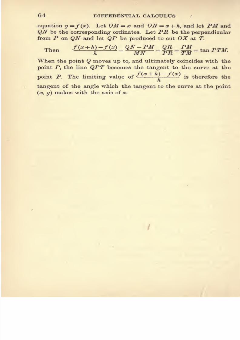
7/27/2019 7-CALCULUS AND PROBABILITY-1922-Alfred Henry.pdf
http://slidepdf.com/reader/full/7-calculus-and-probability-1922-alfred-henrypdf 78/170
64 DIFFERENTIAL CALCULUS /
equation y =/(a?). Let OM — x and ON =x-{-hy and let PM and
QN be the corresponding ordinates. Let PR be the perpendicular
from P on QN and let QP be produced to cut OX at T.
Then/(^ + ^)-/W _ Q^-PM ^ QR __ PMinen
^
ifiV^- PR- TM'^^^^^'
When the point Q moves up to, and ultimately coincides with the
point P, the line QPT becomes the tangent to the curve at the
point P. The limiting value of — ^ ^-^ is therefore the
tangent of the angle which the tangent to the curve at the point
(a?, y) makes with the axis of x.
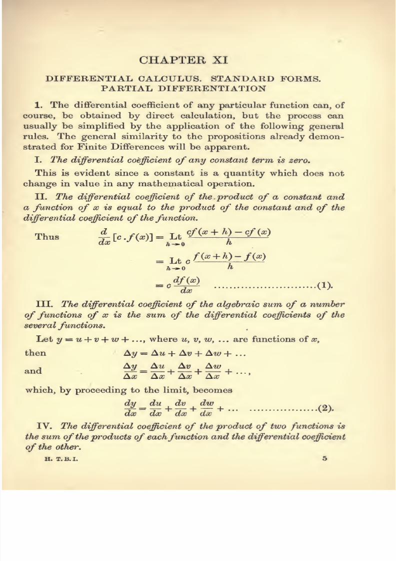
7/27/2019 7-CALCULUS AND PROBABILITY-1922-Alfred Henry.pdf
http://slidepdf.com/reader/full/7-calculus-and-probability-1922-alfred-henrypdf 79/170
CHAPTER XI
DIFFERENTIAL CALCULUS. STANDARD FORMS.
PARTIAL DIFFERENTIATION
1. The differential coefficient of any particular function can, of
course, be obtained by direct calculation, but the process can
usually be simplified by the application of the following general
rules. The general similarity to the propositions already demon-
strated for Finite Differences will be apparent.
I. The differential coefficient of any constant term is zero.
This is evident since a constant is a quantity which does not
change in value in any mathematical operation.
II. The differential coefficient of the product of a constant and
a function of x is equal to the product of the constant and of the
differential coefficient of the function.
Thus #- [c ./(^)] = Lt^/(^+\)-^/(^)
= Lt c
dx ' h^Q
f{x + h)-f{x)
h^O h
-'^ wIII. The differential coefficient of the algebraic sum of a number
of functions of x is the sum of the differential coefficients of the
several functions.
Let y^u-\-v-\-w-\-...y where u,v,w, ... are functions of x,
then Ay •= Au + Av + Aw + ...
^
Ay _ Au Av AwAx ~ Ax Ax Ax ' *
which, by proceeding to the limit, becomes
dy^du^d^^dw_^dx dx dx dx
^
IV. The differential coefficient of the product of two functions is
the sum of the products of eachfunction and the differential coefficient
of the other,
H. T.B.I. 5

7/27/2019 7-CALCULUS AND PROBABILITY-1922-Alfred Henry.pdf
http://slidepdf.com/reader/full/7-calculus-and-probability-1922-alfred-henrypdf 80/170
66 DIFFERENTIAL CALCULUS
Let y = uVy
where u and v are both functions of a;.
Then Ay = (u + Am) (v + Av) — uv= uAv \-vAu + AuAv
= uAv + (v \- Av) Au
^ <^A^ = '*A^ + <'' + ^''>Ai'
whence, taking the limit, when v-^ Av-^v,
dy _ dv du
dx dx dx
which may be written
dy dv du .„^
--^ir^'r^:r^ (3)>
y dx u dx V dx^
This result may be extended to include the product of any number
of functions.
For if y = uvw ; let vw — z, then y — uz.
Whence 1.^ = 1^ + 1^.y dx u dx z dx
P 1 dz _1 dv 1 dw
z dx V dx w dx'
Therefore 1^ =1^+1^ ^l^JH(5).
y dx u dx V dx w dx
Multiplying by uvWy we obtain
dy du,
dv dw ._.
-^ = vw -^ + wu -f- + uv -J- (6).dx dx dx dx
Similarly for the product of any number of functions.
V. The differential coefficient of the quotient of two functions is
(Diff. Goeff. of Numr.){Denr.)-{Diff. Goeff. of Denr.) (Numr.)
Square of Denominator
Let y = --^ v
^ u + Au u vAu — uAvThen . Ay = r =—7
. . ,^ V + Av V v{v { Av)
Au Av. V-r U-r—
, Av Ax Axfl-nd A =—7
ITT }
Ax v{v + Av)

7/27/2019 7-CALCULUS AND PROBABILITY-1922-Alfred Henry.pdf
http://slidepdf.com/reader/full/7-calculus-and-probability-1922-alfred-henrypdf 81/170
STANDARD FORMS 67
whence, taking the limit,
du dv
dy _ dx dx ,^.
di 7' ^ ^'
which may be written
1 dy __1 du 1 dv .^.
y dx u dx V dx '\ r
VI. The differential coefficient of y with respect to x, where y is
a function of u and u is a function of x, is the product of the dif-
ferential coefficients of y with respect to u and u with respect to x.
For 4^^^ ^
whence, taking the limit,
dy^d^dMdx du' dx
^
Similarly
^ =^.*f.*^
(10).*'
dx du dv dx ^
and so for any number of functions.
2. Various standard forms can now be developed, mainly from
first principles. It is instructive to note the points of analogy with
the corresponding forms for Finite Differences.
(i) y = (c^,
dy_^^{x+hY-x^dx h^o h
Lt ^ ^-1
h~^o h
Expanding by the Binomial we have
2=.^J.['^G)^G)^•]
= naf^\ ^
5—2

7/27/2019 7-CALCULUS AND PROBABILITY-1922-Alfred Henry.pdf
http://slidepdf.com/reader/full/7-calculus-and-probability-1922-alfred-henrypdf 82/170
68 DIFFERENTIAL CALCULUS
(ii) 2/= a^
/ = Lt 7
ax \^Q n
= a*Lt J—
= a^'Lt ^ fl + A^ log, a +|'(loge a)» + ... - ll
= a* Lt Tloge a +I
(loge ay + . . .1
= w^ loge a.
If2/ = ^> £ = ^l^g*^ = ^-
(iii) 2/= logad?.
Then ay = x.
Butd(ay) ^djqy) dy
^
dx dy ' dx'
Hence, using the result established in (ii) and remembering that
o^= a;, we have
d^
or
i-''««-l
l=^log«a.g.
Whence dy _ 1
3» a; loge«
Ifrfy 1 1
2' = '°^'^'l'a>\.s,e'-a>-
(iv) 2/ = [/(«')] ; y = e-«»'; y = log. /(«;).
If y=[/w] .
dy dU(x)-r dfjx)
dx df{x) ' dx
Similarly if y = e /W, ^ = e^W . /' (x),
and if y = log./(«). 1=^).

7/27/2019 7-CALCULUS AND PROBABILITY-1922-Alfred Henry.pdf
http://slidepdf.com/reader/full/7-calculus-and-probability-1922-alfred-henrypdf 83/170
STANDARD FORMS 69
(v) y = sm X,
dy _j sin (a? + A) — sin x
dxft^o
^
2 sin ^ . cosHi)
sin
= Lt
2
2 / M
(vi)
Then
whence
Therefore
= cos X,
y = sin~^ X
sin y — x,
dx
dy= cos y = \/l— sin^ y==sll—x^.
c?a?
^ Vl -flj®
*
3. The values of differential coefficients for the other trigono-
metrical functions can be found by methods similarto those employed
in (v) and (vi). The results are given in the table below and should
be verified as an exercise by the student.
FunctionDifferential
CoefficientFunction
Differential
Coefficient
a
loga^?
loge^
sin^
cos 07
tan^
coto?
sec 07
cosec 07
710? -
a* logg a
1
07 log< a
1
07
COS 0?
-sin 07
sec2 x
- cosec^ 07
sec or . tan a;
-cosec 07. cot 07
sin -1 07
COS ^07
tan-^07
COt~l07
sec~^07
cosec~i 07
1
v/l-072
1
1
1+072
1
l+:t2
1
07V07^-1
1

7/27/2019 7-CALCULUS AND PROBABILITY-1922-Alfred Henry.pdf
http://slidepdf.com/reader/full/7-calculus-and-probability-1922-alfred-henrypdf 84/170
70 DIFFERENTIAL CALCULUS
4. Logarithmic Differentiation. This method is of special value
in two cases. Thus if y = uvw , ..
, where Uj v,w, ... are functions
of X, then
logy = \ogu + log v + log w-\- ...,
J 1 dy _1 du 1 dv 1 dw
y dx u dx V dx w dx
dy _ VI du \ dv \ dw ~]
dx~ \ji dx V dx w dx
J'
a result which agrees with that already obtained in § 1.
Secondly if y = w^ u and v both being functions of x,
logy = v log u,
, 1 dy V du , dv
ydx u dx ° dx
dy „ .du „ , dvor -f=^ vu''-^ -J- i-u'lo^u-^.
dx dx ^ dx
5. We will now give some miscellaneous examples of differen-
tiation.
,.. a-\-a^
By the ordinary rule for a quotient
dx (^ + xf
(6 + a;) 2a; -(g 4- a;'') _x''-^2hx-a
\
'^{b + xy (6 + xy '
This can best be treated by resolving the expression into partial
fractions. Then
4 5
y 1-Sx 1 - 2aj
c^y (^ (1 - 3a;)-^ cZ (1 - 3a?) .djl - 2x)--' d(l-2x)
dx~ d(l-Sx) ' dx d(l-2x) ' dx
12 10
(l-3a;)\ (1-2^)'^'

7/27/2019 7-CALCULUS AND PROBABILITY-1922-Alfred Henry.pdf
http://slidepdf.com/reader/full/7-calculus-and-probability-1922-alfred-henrypdf 85/170
STANDARD FORMS 71
(iii) y^^la-\-x. . .
1
dy d(a-\- xY d(a-\-x) 1 , ,--i
ax d{a + X) dx n^
(iv) y = \og{\ogx).
dy __ d log (log x) d (log x) _ 1
dx d (log x) ' dx ~ X log X
'
d {iQic^^ —=======] d,
% _ V V^^ - 1/ ^x'-X d {x - 1)
dx~
1 ' d{p(?-X)' dx
= L_._i(^.2_i)-f.2a;
(v)
1 +
1
a; V ic2 - 1
1
log2/ = -loga?-2--log^-3,
ldy_l d{\ogx-^) d(x-2) ^^^-^ 1
2/ da; a? (i (a; - 2) * rfa?°
a?
l cZ(log^-3) (Z(^-3) ^ 1
1 1 1 . x-~2
~x(x-2) ' x(x-S) x ^^x-S'
Whence ^ - - f^^^T f^
|
iw ^H^l^^^°°^
d^- U-3y U(^-2)(a;-3)^a^^''^a;-3j

7/27/2019 7-CALCULUS AND PROBABILITY-1922-Alfred Henry.pdf
http://slidepdf.com/reader/full/7-calculus-and-probability-1922-alfred-henrypdf 86/170
72 DIFFERENTIAL CALCULUS
(vii) y-a^, h ^,
log y = x log a-\- c^ log b,
^ = a^.h'^ (log a + c* log c log h).
1
(viii) y^af^ + af.
In this case logarithmic differentiation must be used, but for this
purpose the two terras must be taken separately.
Let
1
oF = u and o^ — v.
Thendy _du dv
dx'~ dx dx*
\ogu = x log Xf
Idu 1 .
1
g = ^(l + log^).
Also logw = -loga?,
Idv 1 I , 1
- J- = - . - + log a? . - - ,
V dx X X ^ a?
^ = ^-.-(l-log..).
Therefore -^^ = ar* (1 + log a;) + af~^ (1 - log x).
(ix) Differentiate log^ x with regardto a^.
Let y = loge X and z ^ a^.
Then ^ = ^.^=^.J-.rf^: dx' dz dx' dz'
dx
Therefore ^=- —=—nereiore^^ ^.^^ 2ar»-

7/27/2019 7-CALCULUS AND PROBABILITY-1922-Alfred Henry.pdf
http://slidepdf.com/reader/full/7-calculus-and-probability-1922-alfred-henrypdf 87/170
STANDARD FORMS 73
6. In dealing with cases where a function of two variables is
involved it is convenient to adopt methods similar to those used
in Finite Differences (see Chapter IX, § 4). Thus we define Partial
Differentiation as the process of differentiating a function of several
variables with reference to any one of them, treating the other
variables as constants.
This process is denoted by the symbols o~ » o~ > ^^c. We will also
use the symbol Bx to denote a small change in the value of x.
Let u=f(w,y).
Then u-{-Bu=f(x-\-h,y + k)
and
5w =/(a? +Ky + k)- f{x, y)
_ f{a:-\-h,y-\-k)-f(x,y -\- k) ^ , f {x, y-\rk)-f {x,y)-
h'^^
Ic
' '
Proceeding to the limit when h and k successively -*- 0,
f(x-\-h,y + k)-f{x,y + k) ^dh dx'' ^ ' ^ ^
=^ f(x, y), since A? -* 0.
Therefore hu^:^ .hx \- — . By,dx dy ^
J 8u du du Byand ^ = ^ + ^.-£»
or, when Bx-^0,
Bx dx dy' Bx
du _du du dy ,,^s
dx dx dy' dx
7. If/(a;, 2/)= 0, ^ = Oand
_ du du dy
j
dx dy' dx'
du
Whence ^=-p (12).dx du
dy
Example. If x ^ -^ xy + y^ = 0,
then9^
= 2^ + ^'dy= '' + ^y'
dx x+2y

7/27/2019 7-CALCULUS AND PROBABILITY-1922-Alfred Henry.pdf
http://slidepdf.com/reader/full/7-calculus-and-probability-1922-alfred-henrypdf 88/170
CHAPTER XII
DIFFERENTIAL CALCULUS. SUCCESSIVE
DIFFERENTIATION
1. When -^ is differentiated with respect to a;, we obtain a
further function of x which is known as the second differential
coefficient orsecond derivedfunction of y. This operation
represented
d /dv\ d^vby
-fi-f-jis generally written -r^ or f {x). If the function is
differentiated n times with respect to x, the result is called the nth
d^vdifferential coefficient or nth derived function and is written -j^
Other symbols for the nth differential coefficient are/ *> {x), D^y, y^
2. In many cases the value of the nth differential coefficient can
be found readily by inductive reasoning.
Example 1.
2^= log (a; + a).
_ i_ - 1 _ (- )(- 2) Yy''~x-\-a'y'^''{x^ay'y'~ {x + af '
and by analogy
^ ^ ^>{x +ay
Example 2.
y = a-\-hx->f ca?-\- c?ar» + ...+ kx^,
2/i= h + lcx^- Ma^ -{... -\-n,kx'^-^,
2/2= 2c + 2.3c?a; + ... -h n (n- l)A;a; -^
2/n=
Example 3.
niA;.
7a?-

7/27/2019 7-CALCULUS AND PROBABILITY-1922-Alfred Henry.pdf
http://slidepdf.com/reader/full/7-calculus-and-probability-1922-alfred-henrypdf 89/170
SUCCESSIVE DIFFERENTIATION 75
Making use of the method of partial fractions,
_ 4 5
4.3 5.2yi =
(1-3^)2 (l-2a?)
4.3^.r? 5.2^.yi
^ ^ (1 - 3icf+1 (l-2^)«+i
*
3. Leibnitz's Theorem.
This theorem gives an expression for -^-^ , where y is the product
of two functions of oo, say u and v.
It should be noted first that, as shown in Chapter XI, § 1, the
operator -y- or D obeys the distributive and index laws and is
commutative in regard to constants. In these respects it is similar
to
A (see Chapter II, § 6).
*
XT d , . du dv
and we may therefore write
D (uv) =A (uv) +A (uv)
= (A + A) uv,
where
Aoperates only on u and differential coefficients of u and
A operates only on v and differential coefficients of v.
Therefore
= [A + n D,^-'D, +(2) A'*-'^A^ + . . . + A ] uv.
Now
d^'u
A»M=«^^.,
I),^-'D,(uv) = D,^--'(u^v\ dv d^'^u
dx'^dx''-^'
etc.
Hence
d^ (uv) _ d^u dv d^'^u /n\d^v d^-^u d^dx'' ' dx^^'^'^dx' dx^- -
^W d^* dx -^^' '^
'^dx
(1).

7/27/2019 7-CALCULUS AND PROBABILITY-1922-Alfred Henry.pdf
http://slidepdf.com/reader/full/7-calculus-and-probability-1922-alfred-henrypdf 90/170
76 DIFFERENTIAL CALCULUS
This formula can also be established by induction, but the proof
by this method is left as an exercise to the student.
4. Examples of the application of the formula are given below.
Example 1. y^a^ef^.
Since -t-;^- can be written at once as a**e***, it is convenient to
take a? as the factor v, and e** as the factor u.
Then -j- = Sa?*, etc.
dx
Therefore
Example 2. If y — x^ (log xfy
prove that
ar'2/n+2 + ^n+i = 2 x w .
We have yi = a;** ^ + (log xf n . x ^^
or a?yi = 25?** log x + wa?** (log x)^
= 2a:: log a? + r?2/ (i).
Differentiating both sides of the equation
xyz + yi= h 2 log x . twc** ^ + n^i
X
or ic»2/2 + a?yi = 2ic + 2na? log x + 7ia:ryi
Substituting for x^ log a; from equation (i) we obtain
^y<i. + ^y\ = 2a;** -f nxy-^ — n^y + na;yi
or a^i/a— (2n — l) 373/1 + n'^y = 2a?*» (ii).
By differentiating each term of this equation n times, making
use of Leibnitz's Theorem, we arrive at the result
a^yn+2 4- ?iy„+i.2a;+ w(n-l)y„
-(2w-l)y„+i.a;-n(2w-l)2/„
^yn+2 + a;yn+i =2xnl.

7/27/2019 7-CALCULUS AND PROBABILITY-1922-Alfred Henry.pdf
http://slidepdf.com/reader/full/7-calculus-and-probability-1922-alfred-henrypdf 91/170
CHAPTEE XIII
DIFFERENTIAL CALCULUS. EXPANSIONS.
TAYLOR'S AND MACLAURIN'S THEOREMS
1. It is often necessary to expand f{x) in a series of ascending
powers of x. This has been done by ordinary algebraic or trigono-
metrical methods in such cases as {x 4- a)**, eF, loge(l +x\ sin a?, etc.
The various methods which can be employed may be summarised
as follows:
I. By algebraic or trigonometrical methods.
II. By the use of Taylor s or Maclaurin's Theorem.
III. By the use of a differential equation.
IV. By differentiating or integrating a known series. [For
integration, see Chapters XVI-XX.]
2. I. An example will make this method sufficiently clear.
Examj^le 1. ^^ =^^ / p
t 2^12 720^ *
by actual division.
3. II. Taylor's and MaclauHns Theorems,
Assume that f{x + h) can be expanded in a series of positive
integral powers of h.
Let f{x -\- h) = a -\- bh {- ck + dh^ + ...
Differentiating with regard to h,
f{x + h) = b + 2ch + Sdh^ +...,
f'(x + h)= 2c +S.2dh + ...,
and so on.
Put ^ = 0, then we have
a=/(^), b=f{x\ c=-^\etc.
Hence
/(^+ /i)=/(aj)+A/(^)+|/ (:.)+^/ (^) + ...+^/ )(a;)+....
This result is known as Taylor's Theorem.

7/27/2019 7-CALCULUS AND PROBABILITY-1922-Alfred Henry.pdf
http://slidepdf.com/reader/full/7-calculus-and-probability-1922-alfred-henrypdf 92/170
78 DIFFERENTIAL CALCULUS
4. If in the above result we put a; = we obtain
/W=/(0) + V(0) + |'/ (0)+...+5/(»)(0) + ....
which, by altering the notation, may be written
/W=/(0) + ^/(0)+J/ (0)+ ...+5/»)(0)+ ....
This result is known as Stirling's or Maclaurin's Theorem.
The student should verify the common algebraic and trigono-
metrical expansions by means of the above theorems.
Example 2.
/(«) = log(l +n /(0)= log2,
•
•^ <^> =(T^' / (0) = i,
/ '«=(rTS'/ '(0)=o,
/ W=(1+7;. '
/ (0) = -i,
etc.
Whence, by using Maclaurin's Theorem,
log(l + e')=/W = log2 + |+^-^....
5. The above results are not universal in their application. Thus
it can be shown that the method fails if/(a?) or one of its derivatives
becomes infinite or discontinuous between the specified range of
values of a?. Further, the series obtained must be a convergent series.
Lagrange has shown that the remainder after the first n terms have
been taken from Taylor's series can be expressed as —j/^**^ {x + 6h)y
where ^ is a positive proper fraction. The corresponding value of
x^the remainder in the case of Maclaurin's Theorem is —rf^^U6x).
Unless therefore those expressions tend to vanish when n becomes
infinite, the series is divergent and the methodfails.

7/27/2019 7-CALCULUS AND PROBABILITY-1922-Alfred Henry.pdf
http://slidepdf.com/reader/full/7-calculus-and-probability-1922-alfred-henrypdf 93/170
EXPANSIONS 79
6. III. The use of a differential equation.
The following are examples of the use of this method.
Example 3.
2/= (1 + a;)** = tto + a^x + a^a? + a^a? + ...
Then y^ — n{\+ xY~^ or (1 + x)y^ = ny.
Differentiating the first equation,
2/1= ttj + ^a^x + Za^cc^ + . . .
Therefore
(1 +«;)(« + ^a^x -^ ^a^x^ -\' ...) = 71(^0 + a^x-^ a2X^+ ...).
, Whence, by comparing coefficients,
« = nao,
2a2 + ai = na^f
Sag + 2a2 = nag,
etc.
Puttinga?
= in the original equation we have
ao = l,
and successively
ai = na^ = w,
_(n — 1) _w(7i — 1)a2-—2 «2 '
_ (n-2) _n(w-l)(/i-2)«3-
—3— as-
3j,
etc.
Hence (1 + a;)*^ = 1 + /la; + (g)^ + (3)
^ + ...
Example 4. y == sin ^ ic = ao + aja; + a2x + . ..
1
and (l-x^)yi^=l.
Differentiating (1 - x^) 2y^y^ - 2xy^^ =
or (l-a:»)ya = a^i.
Now sin~^ ic = — sin~* (— x).
Therefore
ao + a^x + a^oc^ ^^ ajo;* + ... = — (a© — Oiic + Oga^ - OsO^^ + ...).
Whence do =^ a, = a4 = . . . = 0.

7/27/2019 7-CALCULUS AND PROBABILITY-1922-Alfred Henry.pdf
http://slidepdf.com/reader/full/7-calculus-and-probability-1922-alfred-henrypdf 94/170
80 DIFFERENTIAL CALCULUS
Thus we may write
yi = ai + M^x'^-\-..,-{-2n-{'l(i^^^aP^ -{-,.,,
2/2= 3 . 2a^{)o + ... + 2m + 1 . 2w . Oan+iaJ^ ^ + ...
Therefore
(l-d?2)(3.2.a8a;+... + 2w + 1.2n.a2n+iaJ*^'+...)=a?(ai+ 3a,ar»+...
+ 2rn-la2;»+iar»»4-...)-
Whence ai = 3 . 2a3,
3a3 = 5.4a5 — 3.203,
(2/1 + 1) O^n+i = (2W + 3) (271 + 2) a^n+s - (27i + 1) 2w . O^n+i
or (2m + ly o^n+i = (2n + 3) (2n + 2) 0^+^.
VBut in the limit when a? -^ 0, - = 1.
Therefore
and accordingly
ai == 1,
03 =1
2.3'
05 =1.3
'2.4.5'
etc.
sin~ ^ X = a; +i^ + L2*3^2.3
.4 5 +nd
7. IV. Differentiation or integration of a known series.
The method is sufficiently indicated by the following examples.
Example 5. sin a; = a? — .- + ^j— . .
.
c^sina; ^ x^ x^
J = cosa? = l-^ + -7-:- ....
dx 2 4
We have therefore obtained the expansion of cos x in terms of x
from that of sin a?.
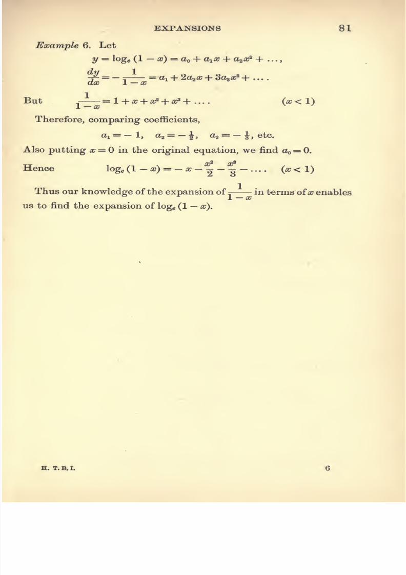
7/27/2019 7-CALCULUS AND PROBABILITY-1922-Alfred Henry.pdf
http://slidepdf.com/reader/full/7-calculus-and-probability-1922-alfred-henrypdf 95/170
EXPANSIONS 81
Example 6. Let
y = loge (1 - a;) = tto + ttia? 4- a.^x'^ + . ..
But =l+a; + d^'2 + a^+.... (^<1)
Therefore, comparing coefficients,
ai = — 1, a2 = — J> a3 = — J, etc.
Also putting a; = in the original equation, we find a^ = 0.
Hence log,(l -a?) = -a;- ^ - 3- ... . («<1)
Thus our knowledge of the expansion of:j
in terms ofa? enables
us to find the expansion of logg (1 — x).
H. T. B. I.

7/27/2019 7-CALCULUS AND PROBABILITY-1922-Alfred Henry.pdf
http://slidepdf.com/reader/full/7-calculus-and-probability-1922-alfred-henrypdf 96/170
CHAPTER XIV
DIFFERENTIAL CALCULUS. MISCELLANEOUSAPPLICATIONS
Limiting Values or Undetermined Forms
1. In certain cases the value of a function cannot be at once
a; — 1ascertained. A common form is illustrated by Lt——^ , the value
of which is not apparent since it takes the form ^ . The function
in this case is said to take an Undetermined or Indeterminate Form,
and since, in the limit, its value is represented by the ratio of two
indefinitely small quantities, it may be expected that the methods
of the Differential Calculus will enable the Limiting Value of the
function to be found.
2. The processto be employed can best be illustrated
byexamples.
Example 1. To find Lt _, .
Let x = l -i-h, then
»-o L f>,
= Lt[n+g)fc + («)/t^+...]
= 71.
Example 2. To find Lt P^^f^ ^^^]
x - a;2
2
a?-f 2 + 3 + -.
Lt 1 — a; 4- 5 ic2 - . . . (by actual division)
t-^^o L ^ J
1,
since the series obtained by division is obviously convergent.
X-
= 1,

7/27/2019 7-CALCULUS AND PROBABILITY-1922-Alfred Henry.pdf
http://slidepdf.com/reader/full/7-calculus-and-probability-1922-alfred-henrypdf 97/170
MISCELLANEOUS APPLICATIONS 83
Example 3. To find Lt ^ ,
= Lt^[/iog^+2i^^ g^)'+--l]
a; log c +|j
(log c)* + . .
.
I log^r
+ {.logo4(Iogc)»+...pi^V
=1^* — ^
T ^qr a;log (QTlogc+ terms involving a °and higher powers ofa?
--*»^log5- + J(logsry+...
_ T i.5^ lo^ j7 1<^R ^+ terms involving x and higher powers ofa;
log5r + |j(log^)^+...
= 5rlogc.
3. The formulas of the Differential Calculus can be used for the
solution of problems of this class, in the following way.
Let, , { take the form ^ when x~*-a.<p{x)
Then if a; = a + A, by Taylor's Theorem,
f(x) ^ f(a)+hf(a)^..,
<f)(x) (j>{a) + h(t> (a)+,./
Therefore, when aj-^-a, and consequently A, /(a) and <\){a) all
-^0, we have
If this is still an undetermined form, the process can be repeated.
Taking Example 3 above, we have
f{x) =g^-g, 4>(x)==g^-h
f(x)=:g^(f\ogg\ogc, <i>\x)^^\ogg.
6—2

7/27/2019 7-CALCULUS AND PROBABILITY-1922-Alfred Henry.pdf
http://slidepdf.com/reader/full/7-calculus-and-probability-1922-alfred-henrypdf 98/170
84 DIFFERENTIAL CALCULUS
Therefore Lt-f-^^Lt^^^^^^^^^^^
= g log c, as before.
4. Other Undetermined Forms are found when a function in
the limit assumes one of the following forms
0x00, — , x-oo, 0 , 00°, or 1 .00
These can all be made to depend upon the form ^
Thus if/(a?) and <^ {x) be the two functions involved, in the first
fix)case by writing /(a?) x 6 {x) aS p/ we have the form ^r and can
L0(a?)J
proceed as before.
Similarly for the second form.
The third form can be written as xj1 [; the second term
within the bracket can then be evaluated, and the quantity within
the bracket will then be found to be zero or otherwise. In the
former event the product is of the form x x and can be evaluated
in the latter event the value of the product is clearly infinite.
The last three cases are solved by taking logs, when the logarithm
of the function will be found to fall within one of the cases already
discussed.
5. In connection with the form 1 , it is useful to rememberthat, from the development of the Exponential Theorem in algebra,
it follows that
A x/Lt
and Lt (l + -) =X
Maxima and Minima
6. lif{x) continuously increases with x until it attains a certain
value a and subsequently decreases, the value a is said to be a
maximum value of the function. Conversely if the value of the
function continuously decreases, while x increases, until it attains
a value h and subsequently increases, the value h is said to be a
minimum value.

7/27/2019 7-CALCULUS AND PROBABILITY-1922-Alfred Henry.pdf
http://slidepdf.com/reader/full/7-calculus-and-probability-1922-alfred-henrypdf 99/170
MISCELLANEOUS APPLICATIONS 85
By this definition there may be several maximum values and
several minimum values; further, a minimum value may con-
ceivably be greater than one of the maximum values.
These conceptions are illustrated in the following diagram.
Thus the points A and B are maxima, whilst the points B and
E are minima. At the point G
the value of the function ceases
momentarily to increase but is in-
creasing both before and after the
point is reached. Such points,
where the rate of increase or de-
crease in the value of the function tends to become constant as the
point is reached, are called points of infleodon.
7. In obtaining criteria for ascertaining the maximum or
minimum values the following considerations are of importance.
If f{x) increases in value with x, it is clear from the definition
that -^ is positive. Conversely if f{x) decreases with Xy -^ is
negative.
Further, if f(x) is continuous and assumes two values /(a) and
/(6), one of which is positive and the other negative, it follows that
for some value of x between the values a and hyf{x) must be either
zero or infinite.
8. Now for a maximum value the function increases up to that
value and then begins to decrease. Therefore at a maximum value
dxi
-p must change from positive to negative ; similarly at a minimum
value-J-
is changing from negative to positive. It follows from the
preceding article that at a maximum or minimum point the
value of-J-
is zero or infinite.
9. Further, at a maximum point -^ is decreasing from positive
to negative, and therefore j^ must be negative or zero. At a
minimum point the converse is the case and -r^ is positive or zero.

7/27/2019 7-CALCULUS AND PROBABILITY-1922-Alfred Henry.pdf
http://slidepdf.com/reader/full/7-calculus-and-probability-1922-alfred-henrypdf 100/170
86 DIFFERENTIAL CALCULUS
Hence in order to find the maximum and minimum values of
f{x) it is necessary
(i) to find the values of x which satisfy the equation /' {x) =
or/'(a?) = oo,
(ii) to ascertain for each of these values whether/ {x) is negative
or positive.
If f {x) = 0, a further test is necessary. For the investigation
of these cases, which include values which give rise to points of
inflexion, the student is referred to more advanced treatises on the
subject.
Example 1. What fraction exceeds its ^th power by the greatest
number possible ?
Let X be the fraction ; we have to find the maximum value of
y = x — xPy
dy
dxj=i-p.^-^
For a maximum or minimum value -i^ = 0, thereforedx
l-pxP-^ = 0,
and ajP ^ = -
i_
or x=p p-^.
Now ^=_^(^_l)^P-2
and is therefore negative.
Hence the above value of a? is a maximum value.
Example 2. What are the dimensions of the largest rectangular
box on a square base the area of whose surface does not exceed
12 square feet?
Let X be the volume of the box, a the length of the base and h
the height.
Then the surface is 2a^ + 4a6 = 12, whence

7/27/2019 7-CALCULUS AND PROBABILITY-1922-Alfred Henry.pdf
http://slidepdf.com/reader/full/7-calculus-and-probability-1922-alfred-henrypdf 101/170
Also
MISCELLANEOUS APPLICATIONS
X = a'b
=a' (6 - a')
2a ~= 3a-
2'
dx_^ 3a»
da
87
dxFor a maximum or minimum value j- = 0, therefore
da
s-¥-oor a = ^2, whence 6 = ^l%
d^x /- . .
and since -j—^ is negative when a = v 2, this value gives a maximum
value for a?.

7/27/2019 7-CALCULUS AND PROBABILITY-1922-Alfred Henry.pdf
http://slidepdf.com/reader/full/7-calculus-and-probability-1922-alfred-henrypdf 102/170
CHAPTEE XV
RELATION OF DIFFERENTIAL CALCULUS TOFINITE DIFFERENCES
1. By Taylor's Theorem we have
But /(a? 4- 1) = Ef{x\ therefore if the operation -7- be denoted by
D we may write symbolically
Ef{x) = {l+D + D'-V. ..)/W
= e^f{x)
or E = e^,
whence A = e^-1
and i) = log,(l + A).
Therefored . A'' A»
5^ = ^-¥ + -3-•1
(1).
If the interval of differencing be h, we have
2f{x + h)^f(x)-^hf(x) + %r(x) +
and therefore A = e^^ — 1.
Further, i)» = [log, (1 + A)]»,
, d^y [^ A' A' 1^whence
_J= ^A-^ + ^ -
...J
2^
= A»y-A»2/ + |iA^2/-fA»y+ (2).
Similarly ^= A'y - ^A'y + iA'y - (3).
2. The above formula (1) gives a convenient expression for the
differential coefficient in terms of advancing differences. But from
the nature of the differential coefficient, it may be expected that a
better result will be obtained by applying the formulas of central
differences.
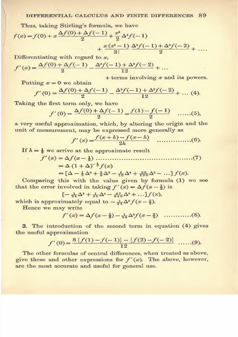
7/27/2019 7-CALCULUS AND PROBABILITY-1922-Alfred Henry.pdf
http://slidepdf.com/reader/full/7-calculus-and-probability-1922-alfred-henrypdf 103/170
DIFFERENTIAL CALCULUS AND FINITE DIFFERENCES 89
Thus, taking Stirling's formula, we have
^3 2^ '
Differentiating with regard to x,
A/(0) + A/(-l) Ay(-l) + A'/(-2)
/ W- 2 12 ^••
+ terms involving x and its powers.
Putting a; = we obtain
y (0)_ A/(0) + A/(- 1) Ay(- 1) + A'/(- 2)
^ ^4^Z Iz
Taking the first term only, we have
^-(0)- V(0) + V(-l) _/(l)-/(-l)
(5),
a very useful approximation, which, by altering the origin and the
unit of measurement, may be expressed more generally as
/'(^)^/(^ + ^)-/(^-^> (6).
If A = J we arrive at the approximate result
- f'(x) = Af(x-i) (7)
= A(1 +A)-VW
Comparing this with the value given by formula (1) we see
that the error involved in takingf {x) — A/(a; — J) is
[- ii^' + iVA^ - /A^^ + • • -l/C^X
which is approximately equal to — ^^^/(a; — f).
Hence we may write
r{x)^^f{x-\)-i^ll^f{x--i) (8).
3. The introduction of the second term in equation (4) gives
the useful approximation
^, (0)8 (/(I) -/(- 1)1 - (/(2) -/(- 2)1
^g^_
The other formulas of central differences, when treated as above,
give these and other expressions for f (x). The above, however,
are the most accurate and useful for general use.

7/27/2019 7-CALCULUS AND PROBABILITY-1922-Alfred Henry.pdf
http://slidepdf.com/reader/full/7-calculus-and-probability-1922-alfred-henrypdf 104/170
90 DIFFERENTIAL CALCULUS AND FINITE DIFFERENCES
4. Using the central difference formula, we shall obtain for the
dififerential coefficients of higher orders,
/ (0) = A^/(-l)-^AV(-2) (10)
and r'(o)=A3/(~l) + Ay(-2)
= Ay(-f)approx (11).
5. An example of the working of the above formulas is now given.
Example. Find the first three differential coefficients of log a;,
when x=2. having given the values of logg 1'80, loge 1*90, ....
NumberNatural
logA A2 A3 A* A5
1-80 •587787 •054067 - -002774 •000271 -•000038 •000007
1-90 •641854 •051293 - ^002503 •000233 -•000031 •000005
2-00 •693147 •048790 - 002270 •000202 -•000026 •0000(34
210 •741937 •046520 - ^002068 •000176 -•000022 •000004
2-20 •788457 •044452 - ^001892 •000154 - ^000018
2-30 •832909 •042560 - -001738 •0001362-40 •875469 •040822 - -001602
2-50 •916291 •039220
2-60 •955511
Using the advancing difference formula (1), starting at the term
2*00, and remembering that the interval of differencing is not unity
but '1, we get
/'(.) = 10 (.048790 +:^+:^^:^^= -50000.
Similarly
/ {x) = 100 (- -002270 - -000202 - {^ x -000026 - f x -000004)
= - -2499,
f {x) = 1000 (-000202 + f X -000026 4- J x -000004)
=-248.
The true values are, of course, given by the differential coefficients.112f log X, which are respectively - , — -i^, -^ . When a? = 2 these
X Sj Xi
become ^, —J, J; the closeness of the above approximations is
apparent.
Formulas (6) and (9) give respectively for/' (x) values of -50042
and -50000.

7/27/2019 7-CALCULUS AND PROBABILITY-1922-Alfred Henry.pdf
http://slidepdf.com/reader/full/7-calculus-and-probability-1922-alfred-henrypdf 105/170
CHAPTER XVI
INTEGRAL CALCULUS. DEFINITIONS
AND ILLUSTRATIONS
1. In Finite Differences we discussed under the heading of Finite
Integration the problem of finding the value of /(O) +/( ) + ...
+f{n - 1), or, changing the origin and the unit of measurement,
the more general series
^ [/(«) +/(« + ^) +/(» + 2/i) + . . . +/(a + rT^rr/^)].
The Integral Calculus deals with the value which this summa-
tion assumes when h becomes indefinitely small.
2. Now let F{x) be a function such that f{x) is its differential
coefficient. Then by definition
or
where Wi is a quantity that vanishes when ^^-0.
Then we have
hf(a) =F(a-{-h) -¥{0) \-ha^,
hf(a + h) =^F(a + 2h)-F(a-{-h) -hha^,
hf(a-\-2h) = F(a + Sh)-F(a + 2h) +has,
hf(a + n-lh):=F(a-^nh)-F(a-^n-lh)-^ hon.
By addition,
h [/(a) +/(o^
+A) 4-/(a
+2A) 4- . . . +/(a
+n - \h)]
= -F (a + n/i) - i^ (a) + ^ [« + 02 + . . . + «„].
Now if a denote the greatest of the quantities ai, ctj, ... ««, the
last term is clearly less than nha, or (h - a) a, if a + nh be put equal
to h. This term therefore vanishes in the limit and we are left with
the relation

7/27/2019 7-CALCULUS AND PROBABILITY-1922-Alfred Henry.pdf
http://slidepdf.com/reader/full/7-calculus-and-probability-1922-alfred-henrypdf 106/170
92 INTEGRAL CALCULUS
This result is usually expressed in the form
'f{w)dx^F(h)-F{a),I
where F{x) is a quantity such that /(a?) is its differential coefficient
and dec represents, in the limit, the indefinitely small interval
between the terms which are summed.
The expression I f(x) dx is called the definite integral of f{x)J a
with regard to x, and h and a are called respectively the superior
and inferior limits of integration.
Where no limits to the summation are expressed and we are
concerned merely with the form of the function, we obtain the in-
definite integral.
3. A geometrical illustration of the process of integration may
be obtained as follows.
Let the equation y=f(x) be represented by the curve in the
diagram. Let OA = a and OB = 6, so that ^
MA^fia) and NB = /{b).
Further, let AB he divided into n parts
each equal to h. Then the sum of the rect-
«=6M
B
angles shown is clearly equal to S hf(x), and,x=a+h
in the limit, when h^-0 the value of the
integral becomes equal to the area between the curve and the axis
of X bounded by the ordinates MA and NB.

7/27/2019 7-CALCULUS AND PROBABILITY-1922-Alfred Henry.pdf
http://slidepdf.com/reader/full/7-calculus-and-probability-1922-alfred-henrypdf 107/170
CHAPTER XVII
INTEGRAL CALCULUS. STANDARD FORMS
1. In the preceding chapter we found that the process of integra-
tion is the converse of that of differentiation. In other words, that
given /'(a?) we have to find a function f{x) such that f (x) is its
first differential coefficient. The analogy with the process of finite
integration is apparent and the remarks made in Chapter VII,
§ 5, apply equally to the present case.
It may, therefore, be said again that the process of integration
cannot be carried out for every function, that definite rules cannot
be laid down to apply in every case, and that the student must look
to applying the results of the differential calculus as a guide in
solving any problem presented by the function under consideration.
2. In the first placeit is
necessary to point out that the ordinaryalgebraic laws apply to the integrating symbol jdx in the same way
as they have been shown to apply to the symbolic operations A and
I-. Thus:ax
(1) The operation is distributive for, ii u,v, w,...he any func-
tions of Xy
-^\\udx-{- \vdx-\- jwdx + ...h = w + t; + w...
and therefore
\udx-\- jvdx+ \wdx-^..,= l(u + v-\-w-\- ...)dx ...(1).
(2) The operation is commutative with regard to constants, for,
.„ dv d(cv) ^cdv_
dx~*
dx dx *
therefore Icudx^cv^c ludx (2).
3. It should be added that the process of integration introduces
dva constant into every indefinite integral, for, i£ u = -t- ,
div-^-c) _dv__
dx ~ dx*
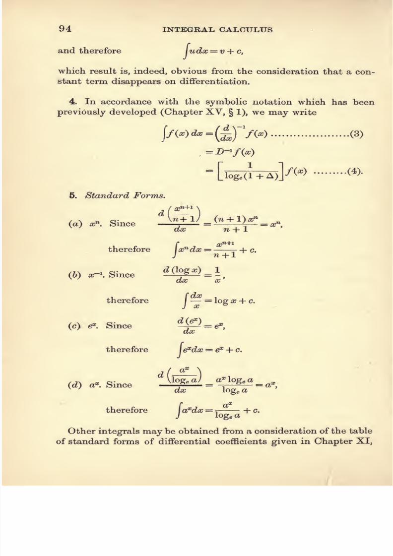
7/27/2019 7-CALCULUS AND PROBABILITY-1922-Alfred Henry.pdf
http://slidepdf.com/reader/full/7-calculus-and-probability-1922-alfred-henrypdf 108/170
94 INTEGRAL CALCULUS
and therefore ludx = v + c,
which result is, indeed, obvious from the consideration that a con-stant term disappears on differentiation.
4. In accordance with the symbolic notation which has been
previously developed (Chapter XV, § 1), we may write
lf<-^^-{iTf(-) (3)
=[WTA)]^(^>
^'^-
6. Standard Forms.
(a) x^. Smce = = -^^ ^— = x^,
therefore lx'^dx = + c.
J w+1
d([ogx) 1(6) x-\ Since
dx x
dxtherefore /— = log a; + c.
(c) e^. Since
therefore
d{f)
dx
\^dx = € ^-\-C,
d(-^](d) a*. Since -js = -j—^— = a*,
therefore I a'^dx=^
1- c.
j logea
Other integrals may be obtained from a consideration of the table
of standard forms of differential coefficients given in Chapter XI,

7/27/2019 7-CALCULUS AND PROBABILITY-1922-Alfred Henry.pdf
http://slidepdf.com/reader/full/7-calculus-and-probability-1922-alfred-henrypdf 109/170
STANDARD FORMS 95
§ 3. The results are embodied in the following table. Their verifi-
cation is left as an exercise to the student.
Function Integral
Ix^'dx
^+1
J 3C
log,:P
\a^dxa'
log, a
\^dx eP
1cosxdx sin^
jainxdx -cos^
1
aec^xdx tamx
1cosec^ X dx -cot a?
In each case the constant c has been omitted for the sake of
simplicity, but its importance in the result must not be forgotten.
6. Sums of the above functions can be integrated by the use of
the distributive property of the operation of integration. Thus
[{w + 2^^) da; = jx^ dx +12^ dx
X 2^
l0ge2+ C.
Similarly (ax^ + bx~*) dx=a jx*dx + b lx~*dx
oaf
5
hx'+ c.
7. The problem of integration may be presented in another way.
Thus to find the sum of
1
X x +m x + 2m
when X is indefinitely increased.
+ ...+1
x + xm

7/27/2019 7-CALCULUS AND PROBABILITY-1922-Alfred Henry.pdf
http://slidepdf.com/reader/full/7-calculus-and-probability-1922-alfred-henrypdf 110/170
96 INTEGRAL CALCULUS
The series may be written as
+ ...+1 rl 1 1
1 .
m^ 2m1 + - 1 +
X X\+x m
m
X
The terms in the denominator consist of values of a quantity, which
mcan be represented by y, increasing by equal increments of— . Also
X
the sum of the series is multiplied by — , which is the incrementX
in the value of the denominator.
Since the initial value of the denominator y is unity and the
final value is 1 + m, from our definition of an integral we may write,
when a7-» oo and therefore—^0.X
Lt - Y + + T-+--- +
1 + - 1 +— l-\-x.-\
X X X
dy
ymJi
mlog 1 + m.

7/27/2019 7-CALCULUS AND PROBABILITY-1922-Alfred Henry.pdf
http://slidepdf.com/reader/full/7-calculus-and-probability-1922-alfred-henrypdf 111/170

7/27/2019 7-CALCULUS AND PROBABILITY-1922-Alfred Henry.pdf
http://slidepdf.com/reader/full/7-calculus-and-probability-1922-alfred-henrypdf 112/170
98 INTEGRAL CALCULUS
(3) [(h + 2cx) (a + hx + ca^f dx.
Put a-\-bx + cx^ — y.
Then (6 + 2cx) dx = dy.
Therefore
[(h + 2cx) (a + 6a; + car*)** dx=\y''dy = ^—- + k
=n+l
+*•
(4)
(log x)^ dx
J X
Put logx^y.
Then ~dx= dy.X
Therefore
•(log
•X
dx=jrdy l^^+o
_(log.^)''«
n + \
(5)
Put /W=y-Then f'(x)dx=dy.
Therefore
(6) /^.Put a^ = y.
Then 2xdx = dy.
-4/*-/i?-J
= Hy-logl+3/] + c
= J[ar»-logrT^] + c.

7/27/2019 7-CALCULUS AND PROBABILITY-1922-Alfred Henry.pdf
http://slidepdf.com/reader/full/7-calculus-and-probability-1922-alfred-henrypdf 113/170
0)
PutThen
Therefore
METHODS OF INTEGRATION
sin xdx
99
r siE
J a + bcoax'
a +6 cos
x=
y.
— h sin xdx = dy.
C sm xdx 1 fciy 1 , . loe^ (a + 6 cos x)
J a-{-bcoax bj y b ^^ b
(8)
y
r dx _sin a?
[dx
c.' X X
2 Sin 2 COS 2
sec'^ ^ dx
. 2tan|
Put tan2 = y.
Then J sec'^ 2<^^ = dy-
Thereforef dx
_
J sin a?
~
= logtan| + c.
Corollary. Since
cosaj = sm(|+a;j,
hdx
,osa7
= lo^?tang +|)+ c
II. Rationalisation by Trigonometrical Transformation
3. The above methods can be extended by the use of trigono-
metrical functions and the relations which exist between them.
The following are examples
(1)
Let
Then
and
r dx
a; = a sin y.
dx = a cos ydy,
Va^ — a^=acosy.
7-2

7/27/2019 7-CALCULUS AND PROBABILITY-1922-Alfred Henry.pdf
http://slidepdf.com/reader/full/7-calculus-and-probability-1922-alfred-henrypdf 114/170
100 INTEGRAL CALCULUS
Therefore,
= \dy=iy-\-c
— sin~i - 4- c.a
(2) \-J^^^
Let a;= a sec y.
Then dx=a8ecy tan ydy,
and sia? — a? — a tan y.
Therefore
[_^ = [^ = log tan (j + D+c
l+tan|
= log -4-c
l-tan|
, 1 + sin3/ ,
° cos2/
7' -I./2
= log 1- c
='°gi ^— ) +
''•
Let a? = a tan y.
Then dx = a sec'' 2/d 2/,
and Var^ ^a^ = a sec y.
Therefore
r_^ = f^ = logtan(j + |)+cJv^Ta' J cos 2/ ^ \4 2/
= log (sec 3/ + tan 2/) + c [See Ex. (2)]
=log(^±^')+c.

7/27/2019 7-CALCULUS AND PROBABILITY-1922-Alfred Henry.pdf
http://slidepdf.com/reader/full/7-calculus-and-probability-1922-alfred-henrypdf 115/170
METHODS OF INTfiGRV^tiW 101
From the above integral, two ©thef . fenpc^'stifb . jjb^eC. phn be
obtained.
(4) (
^^
J ^/a-\-2bx-hcaf'
This can be written as
da: f d {cx + 6)
/{cx^hf-\- r/c-¥ J Vc {(ca; + hf -\-ac- t^j
Disregarding for the moment the constant multiplier, this can
clearly be transformed into one of the forms given in Examples
(1)_(3) above.
Corollary. Since
I= 2 log ( Jx-a + Va? - 6) + c,
f dx ^.
^ Ix — a=r = 2 sm-^ A / f- + c.
J ^/{x-a){b-x) Vb-a
l^B + cx) + ^P^^^^
J Na->f
(p + qx) dx _
2bx + cx^ s/a + 2bx + cs?
dx
_ q C d(a-h2bx + cx ) (pc- qb)f
dx
~2cJ Va + 2bx + c^2 c JVaT26^Tc^*
The value of the first integral is 2 (a + 2bx + cx^)^ and the second
integral can be dealt with as in Example (4).
4. General remarks in regard to the method of substitution.
When the precise substitution which will enable the integral to
be solved is not apparent the device illustrated in the following
examples is often of assistance.
(x + a) dx(1) 1,4(x +
The appropriate substitution is not apparent, so assume
where r may have any value, to be determined subsequently.

7/27/2019 7-CALCULUS AND PROBABILITY-1922-Alfred Henry.pdf
http://slidepdf.com/reader/full/7-calculus-and-probability-1922-alfred-henrypdf 116/170
102 ;;
;V / 3[|T.*EGRAL CALCULUS
Th^wf :/; :;f /''/:;; \xi^b^y^
and dx^2ry'^^dy.
The integral thus becomes
r {y'^ + a-c)2ry'^-'dy
J (y2r^l,_c)y^'
Clearly this integral can be evaluated if y^ = y^''-\ i.e. if r = 1,
when we get
^ ^
a — h , y-^Jc — h,= 2y + -7==. log ^^ 7=+ A;,
Vc-6 =
y + ^c-b
where y=i^x + c. •
(2) f ^ ^
Let us take the linear function as likely to lead to simpler results
and, as before, put
x — p = y^
so that dx = ry^~^dy.
Then the transformed integral is
r rif~^dy C rdy
J y Va + 26 (y*+i)) + c (y' + pf Jy \/a + 26 (y''+p) + c (y^'+pY
*
Obviously if r = — 1, the denominator reduces to the form
and theexpression
can be immediately integrated.
(8) f-^.This example is a little more difficult than the two previous
ones. As before, let x = y^, so that dx = ry^^ dy. Then we have
dxfry'^^dydx r ry'^^dy

7/27/2019 7-CALCULUS AND PROBABILITY-1922-Alfred Henry.pdf
http://slidepdf.com/reader/full/7-calculus-and-probability-1922-alfred-henrypdf 117/170
METHODS OF INTEGRATION 103
The expression within the brackets in the denominator is of an
even degree in y, so we will express the integral in the form
rfd{y^)ryr-'d(f) _f
2y^^ {ay-^ ^^ cf
This can clearly be integrated if r — 2 = 3r, when r = — 1. The
integral then becomes
_1 { df ^ 1 r d{af + c) __ 1
^^j^
a (a + cx^f+ k
5. Definite Integrals. The above examples of the application of
the method of substitution all relate to indefinite integrals and the
final form of the indefinite integral is expressed, in each case, in
terms of oo.
In the case of a definite integral, a step may be saved in the
operation by avoiding the final substitution of x in terms of y,
provided appropriate changes are made in the values of the limits
of integration. An example will make the point clear.
r> 7 r^^dx
Example,\ ,
• .^h'Jl+x'
Put a;2 = y.
Then 2xdx=dy.
Also when x =0, y=0 and when a; = 2, ^ = 4.
Thus we get
III. Integration by Parts
6. From the Differential Calculus we have
d (uv) __ dv du
dx dx dx'
Whence, by integration,
uv = \u-J-
dx + \v-T- dx,

7/27/2019 7-CALCULUS AND PROBABILITY-1922-Alfred Henry.pdf
http://slidepdf.com/reader/full/7-calculus-and-probability-1922-alfred-henrypdf 118/170
104 INTEGRAL CALCULUS
f dv ^ f du ,
or lu-^ ax = uv — Iv-rr- dx.J dx J dx
Consequently an integral of a function of the form u-i-
can
always be made to depend upon that of a function of the form v -3-.
The latter may prove to be a standard form and the use of the
formula given above may enable an apparently intractable ex-
pression to be integrated at once.
The advantage of the method is best exhibited by applying it to
a few elementary cases.
(1) jx\ogxdx==^j\ogx-^dx
= ^x^\ogx — ^ Ixdx
= ^xHogx--^-\-c,
(2) 1^^''^=^/^^^^
a I a\
(3) /sin-^xdx=l sin ^ x-^- dx
. , r d(sm~^x),= a;sm~^a;— jx , -d^
., f xdx
= X sin~^ X —I ,
= X sin~^ a; + Vl — a? + c.
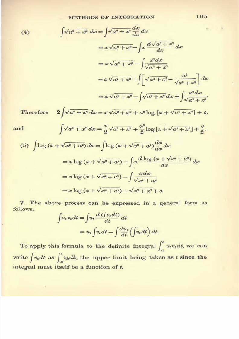
7/27/2019 7-CALCULUS AND PROBABILITY-1922-Alfred Henry.pdf
http://slidepdf.com/reader/full/7-calculus-and-probability-1922-alfred-henrypdf 119/170
METHODS OF INTEGRATION 105
dx, dxax4) Ua? + x dx = j*Ja^T^
,— r d^/a^ + x ,
==x^a^ + x^-jx—2 '^
, f a^dx^x^a^' + x'- I
,,
j\_ Na?-\r a?}
r rQ/^cix
J J^/a' + a^
Therefore 2 /VoM^dx = x Va^ + x^ + a^ log [x + Va^ + x ^] + c,
and j\/aFT^dx = | VoM^ + ^ log [a;+VaM^] + 1 •
(5) / log (x + ^x + o?) dx= flog (x + V^M^^) ^^
=:.iog(.+vSM:^)-/^^
= ic log (x + Vic^ + a ) -V^T^+ c.
7. The above process can be expressed in a general form as
follows:
= ut jvtdt - I -Jilj'^tdtj dt.
To apply this formula to the definite integral I UtVtdt, we canJ a
write \vtdt as I Vkdk^ the upper limit being taken as t since the
integral must itself be a function of t

7/27/2019 7-CALCULUS AND PROBABILITY-1922-Alfred Henry.pdf
http://slidepdf.com/reader/full/7-calculus-and-probability-1922-alfred-henrypdf 120/170
106 INTEGRAL CALCULUS
Thus we get
/ UtVtdt = wj Vkdk —{-Tfi] Vkdkj dt
= UbI
Vkdk — Ua I Vkdk — I -— i Vkdkj dt
= UbI
Vkdk— -^ { I Vkdk\ dt,
since / Vkdk = 0.
J a
Alternatively, if we express Ivtdt as the definite integral
— I Vkdk, we obtain
UtVtdt = Ub I Vkdk-\-j -T^ij Vkdkjdt*.
8. Reduction Formulas. Where integration by parts is not im-
mediately successful, continuation of the operation may ultimately
lead to the evaluation of the integral.
Thus (x'e'dx =ja^^dx=:a^e'-je''^dx
(xe^ - I e^dxj
= x^e^-2 ler^xdx
d^ ,
x-^- axax
^x^e'-l
= a;2e*-2a;e^ + 2e=^ + c.
9. The above case is an example of a Reduction Formula, this
designation being used since the application of the method of
Integration by Parts efifects the reduction by successive steps of
one term in the integral.
Thus
[x^a- xY dx ='^'^'^'
^^ ;^^'^
+ \^^ nil- x)^'' dx.
i ^ ^ m+1 jm+1 ^ ^
* See J.I.A. Vol.44, pp.
402-409.

7/27/2019 7-CALCULUS AND PROBABILITY-1922-Alfred Henry.pdf
http://slidepdf.com/reader/full/7-calculus-and-probability-1922-alfred-henrypdf 121/170
METHODS OF INTEGRATION 107
Thus the degree of the term (1 — x)^ has been reduced by unity.
Successive applications of the formula will reduce the degree
further, until, if n is an integer, the term ultimately equals (1 — xfor unity.
In the special case where the value of this integral is taken
between the limits and 1, we have
x'^(l-x)''dx=\
-(l-xY\ + :rn(l-x)''-^dxJo |_m + l^ ^Jo Jom-\-l
=-^ r a;^+i (1 - xY-^ dx,
whence by successive applications of the formula we find ulti-
mately if n be an integer that
Ix'^Ci-xYdx^ r x^'^'^dx^ -,.
Jo 7i-f-m .'o n + m+1
Many other important integrals can be dealt with in a similar
way.
IV. Integration by the use of Partial Fractions
F (x)10. Any expression of the form ^ . , where F{x) and /(a?) are
both rational integral algebraic functions of x, can be expressed as
the sum of a number of terms of which the general forms are arX^
and '—^^-. For if the degree of F{x) is equal to or greater than\X — Cr)
that oi f{x), by division we can obtain a quotient, together with a
new fraction in which the numerator is of lower degree than the
denominator. The quotient provides the terms of the first form and
the new fraction can be split up by partial fractions into terms of
the second form. The integrals of these general forms are known
and consequently the whole expression can be integrated.
The following are examples
J {x — a){x — o) a — hj\_x — a x — b]
=^;3^
[{aq +i>) log {x-a)- (bq -\-p) log (x - 6)] + c.
^^^Jaa^-h2b.bx + c a
dx
(-n)
ac
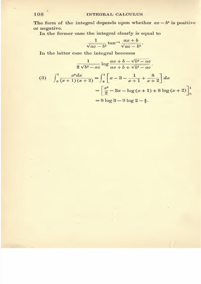
7/27/2019 7-CALCULUS AND PROBABILITY-1922-Alfred Henry.pdf
http://slidepdf.com/reader/full/7-calculus-and-probability-1922-alfred-henrypdf 122/170
108 INTEGRAL CALCULUS
The form of the integral depends upon whether ac - IP is positive
or negative.
In the former case the integral clearly is equal to
1 , , ax-{-h
,tan~^ . .
Nac - ¥ vac - b^
In the latter case the integral becomes
1 , ax + h- V62 - ac
^sly-ac ax + b + y/b^-ac
= \'^-'Sx^\og{x + l) + S\og(x + 2)Y
= 81og3-91og2-|.

7/27/2019 7-CALCULUS AND PROBABILITY-1922-Alfred Henry.pdf
http://slidepdf.com/reader/full/7-calculus-and-probability-1922-alfred-henrypdf 123/170
CHAPTER XIX
INTEGRAL CALCULUS. DEFINITE INTEGRALS.
MISCELLANEOUS APPLICATIONS
General Propositions
1. It is desirable to place on record several general propositions,
in regard to change of limits, which are in the nature of being
self-evident.
In Chapter XVI it has been shown that
J a
where /(ic) is the differential coefficient of F(x).
It follows that
I. i''f(x)dx^rf(z)dz (1).
since neither x nor z occurs in the result.
IL l'f(x)dx==-(y(x)dx (2).J a J b
Thus the interchange of the limits results in a change of sign of
the definite integral.
On the left-hand side we have regarded the increment of c^ as
positive, so that, while x increases from a to b, the value of the
integral is F(b) - F{a).
On the right-hand side the increment dx is negative and x
decreases from h to a, giving a value for the integral of
F(a)-F(h).
IIL rf{x)dx=rf(x)dx+( f{x)dx (3).J a J h J a
For the left-hand side is F{c) — F{a) and the right-hand side is
Fie)- F {h) + F {}))- F {a).
IV. \y{x)dx=\y{a^^(p)dx (4).
Jo Jo

7/27/2019 7-CALCULUS AND PROBABILITY-1922-Alfred Henry.pdf
http://slidepdf.com/reader/full/7-calculus-and-probability-1922-alfred-henrypdf 124/170
110 INTEGRAL CALCULUS
For if we substitute a — z for x, then when x = a, z = 0, and when
x=0, z = a.
Also —dz = dx.
Therefore
{ fix) dx = [ -/(« -z)dz= \'f(a - z) dz (by II).' J a JO
=I f(<^ - ^) d^ (by I)-
Jo
2. Differentiation of Definite Integrals.
Let w =I
/(a;, c) cZa?
be a definite integral where the quantity c is independent of x,
and the limits a and 6 are independent of c.
To find -T- let Aw be the change in u corresponding to a change
Ac in c. Then, since the limits are unaltered,
rb
Au = I {/{x, c + Ac) —f(x, c)} dx.
Therefore^y ^ rM/(^, c + Ac)-/(.. o)}^^
Ac Ja Ac
Proceeding to the limit, we have
du
dc =/:«s^'- <«
Thus the differential of the definite integral is reached by a
process of differentiating under the sign of integration.
3. An important use of this theorem is that of finding the values
of other integrals from those of known form.
For example, if the equation
Joe- '^ dx — -
a
* The student is referred to more advanced treatises for exceptions to this
general result,

7/27/2019 7-CALCULUS AND PROBABILITY-1922-Alfred Henry.pdf
http://slidepdf.com/reader/full/7-calculus-and-probability-1922-alfred-henrypdf 125/170
MISCELLANEOUS APPLICATIONS 111
be differentiated n times with respect to a, we get
Jo
n\^n Q-aoi
fjl^ ^ _^ ^
n+i
/,
4. Areas of Curves.
It has been shown that geometrically the definite integral
f{x)dx represents the area enclosed between the curve y=f(oo)
and the axis of x bounded by the ordinates x = a and x = b.
Example 1. Prove that the area of the parabola
2/2 = Asax bounded by the curve, the axis of x andany ordinate is two-thirds of the rectangle con-
tained by the ordinate and the intercept on the
axis of X.
LetO]Sr=b.
Then area OFN=jydx = f '^'^axdx = 2a2 U a;t
= f(2aH^)6
= f rectangle.
5. Mean Value and Probability.
Definite Integrals can be used to find the mean value of afunction whose value is changing continuously by indefinitely
small increments.
Thus to find the mean value of f(x) for all values of x from a to b.
If we divide b — a into n portions each equal to h, the mean value
of the functions /(a), f(a \-h),... f(a-^n— Ih) is
/(a)+/(c^ + ^)+ ... +f(a + n-lh)
^ h [/W +/(« -f^) + ...+/(a + n- Ih)]
b — a
since nh = b — a.
If now we make h indefinitely small, we shall have the mean
value of all values of /(x) from f(a) to f(b). Consequently the
mean value is
1 r»
dx.

7/27/2019 7-CALCULUS AND PROBABILITY-1922-Alfred Henry.pdf
http://slidepdf.com/reader/full/7-calculus-and-probability-1922-alfred-henrypdf 126/170
112 INTEGRAL CALCULUS
Example 2. A number n is divided at random into two parts; find
the mean value of their product.
Let X be one part, then the product is a; (w — x). We have to
find the mean value of this product for all values of x from to n.
Thus we get for the mean value
- x{n-x)dx = -[ — - — ]=-6
6. The class of problem in Probability that admits of being
treated by the methods of the Integral Calculus can best be
illustrated by an example.
Example 3. Three events A, By G are known to have happened
in the same century. What is the chance that the events happened
in the order A, B, G\ B happening within n years of the middle of
the century?
The chance that the events happened in the order A, B, C '\%
clearly ^, if there is no limitation as to when B can happen, since
there are six possible orders in which the events A, B, C can
happen.
To ascertain the further chance that, with the events occurring
in that order, J5happened within n years of the middle of the century,
let X be the number of years from the beginning of the century
to the event B, so that B occurs during the interval of time between
X and X + dx. Then the A cases may have occurred in any of these
X years, and the G cases may have occurred in any of the following
100 — a; years. The total number of possible cases is therefore
X (100 — x) in respect of the above interval of time dx.
But B must have occurred within n years of the middle of the
century, therefore x can have any value between 50 — n and 50 + n.
Hence the required chance, being equal to the number of favour-
able cases divided by the whole number, is
r&O+nx(100-x)dx^ , ^,
I x{100 — x)dxJo
and the answer to the question is
eKi^) Km) ~2 [lOOj 3 VlOoJ

7/27/2019 7-CALCULUS AND PROBABILITY-1922-Alfred Henry.pdf
http://slidepdf.com/reader/full/7-calculus-and-probability-1922-alfred-henrypdf 127/170
MISCELLANEOUS APPLICATIONS 113
7. An example of a somewhat dififerent type is given in the
following problem.
Example 4.
Anevent has always happened on an average once
a year. Find the chance that it did not happen in a given year and
prove it equals e~\
The event has happened on an average once a year. The chance
that it occurred in any given ?ith part of a year is, therefore, - , andn
the chance that it did not occur in that period is 1—By the ordinary rules of probability, the chance that it failed to
occur in n consecutive periods each of -th part of a year is
1—J
. To obtain the solution to the problem, we proceed to the
(1\**1— 1 , which by algebra equals e \
nj
H. T.B.I.

7/27/2019 7-CALCULUS AND PROBABILITY-1922-Alfred Henry.pdf
http://slidepdf.com/reader/full/7-calculus-and-probability-1922-alfred-henrypdf 128/170
CHAPTER XX
APPROXIMATE INTEGRATION
1. In many cases integration, or continuous summation of the
values of a function, cannot be accomplished, either because the
quantity to be integrated cannot be expressed as a mathematical
function, or because the function itself is not capable of being
integrated directly.
In these cases formulas of approximation can be used, which may
conveniently be divided into two classes, viz. formulas expressing
the value of the definite integral in terms of
(i) the sum of the successive values of the function and of its
derivatives,
or (ii) the values of isolated values of the function, not necessarily
successive.
We shall now proceed to consider formulas of the first of these
2. The Euler-Maclaurin Expansion.
Let tf(x) = F(w),
so that f(x) = AF(x).
Then I'
f(x) =/(0) +/( ) + ... -^f(n - 1)
^F{n)-F (0). [See Chapter VII, § 4]
Now J^(a;) = A-i/(a?)
= (e^-l)-»/(a;), since A = e-»-l,
which, by actual division,
=|/(a;) dx - yicc) + ^f {x) -^f {_x) + ....
Therefore
F{n)-F (0)=//W dx - J [fin) -/(O)) + ^V (/' («) -/' (0))
-Ti^l/ '(«)-/ '(0)} + -
But F{n) -F(,0) =/(0) + /(I) +...+f(n- 1).

7/27/2019 7-CALCULUS AND PROBABILITY-1922-Alfred Henry.pdf
http://slidepdf.com/reader/full/7-calculus-and-probability-1922-alfred-henrypdf 129/170
/,
APPROXIMATE INTEGRATION 115
Hence
J{x)dco=y(0) +/( )+...+/(„ - 1)+ J/(n)-fj {/' (n)-/'(0)}
+ tItt {/' «-/' (0)1 -... (1).
This result is not limited to the case where the ordinates are at
unit distance apart, for, as has been remarked in connection with
Finite Differences, by changing the origin and unit of measurement
the formula can be given a more general form. Thus
A f{ c)dx = if(a) +f{a + r)+... +f(a + » - Ir) + }/(a + nr)
- i^r {/' {a + nr) -/' (a)) +^ f/' (a + nr) -/' (a))
-i6f-^'''( + ''''> -^'''('*)' + (2).
r25 ^/p
Example. Calculate —J20 ^
Taking values at unit intervals we have, remembering that
dx i ^^^6
/:
dx
X
1
2'
1 1 1
20 ^
21 ^22
= ^025000•047619
•045455
•043478
•041667
•020000
+A+1 1
24 ^2-
25 12 V
^120 i
1
25*
1
25* 20V
•223219 -iV (-0009) + -^\^ (00000369)
= -223144.
The value of the integral is clearly equal to loge |§, which to
five places of decimals is '22314.
3. Woolhouse's Formula.
This formula gives a relationship between the sum ofconsecutive
ordinates and the sum of equidistant ordinates at greater intervals.
It can be derived from the Euler-Maclaurin formula as follows.
8—2
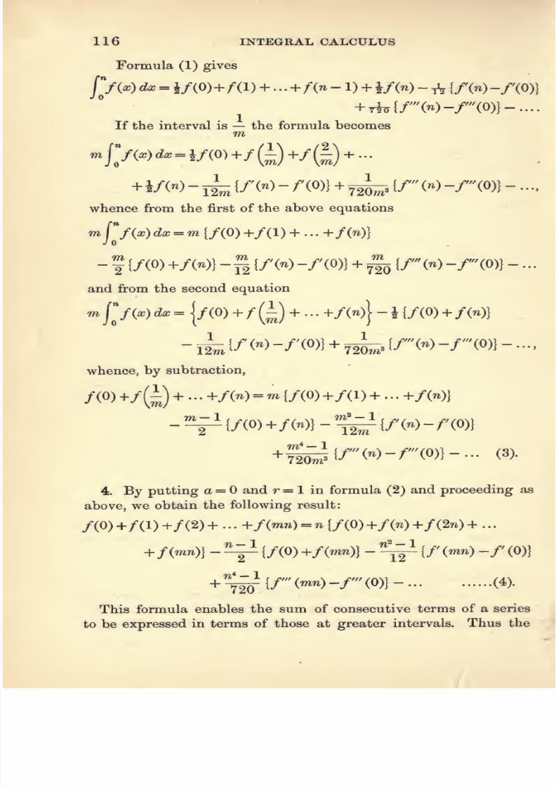
7/27/2019 7-CALCULUS AND PROBABILITY-1922-Alfred Henry.pdf
http://slidepdf.com/reader/full/7-calculus-and-probability-1922-alfred-henrypdf 130/170
116 INTEGRAL CALCULUS
Formula (1) gives
jy(x)dx = y(0)+f(l) + ... + f(n-l) + if(n)-^{f(n)-/XO)}
+ Tkf/ '(»)-/ '(0))-....
If the interval is — the formula becomesm
«/V(.)cte=i/(0)+/(i)+/g) + ...
whence from the first of the above equations
m r/ix) dx = m {/(O) +/(1) + . . . -\-f(n)}Jo
-f
{/(O) +/(«)) -^ l/'W -/'(O)} +^ {/' («) -/' (O)) - ...
and from the second equation
mjy(,x)dw= {/(O) +/(i) + ... +/(«)| - J {/(0) + /(n)}
-i 1/« -/'(«>i + 72L. /' « -/' wi- •
whence, by subtraction,
-
^{/(O) +/(«)} -'^ {/« -/'(O))
+f£J(/ 'w-r(o))-... (3).
4. By putting a = and r=l in formula (2) and proceeding as
above, we obtain the following result:
/(O) +/(1) +/(2) + . . . +/(m») = n (/(O) +/(w) +/(2») + . .
+/(™»)1 -^ {/(O) +/( »«)) -'^ {/' («*») -/' (0)1
+ ^{/ '(™»)-/ '(0)}- (4).
This formula enables the sum of consecutive terms of a series
to be expressed in terms of those at greater intervals. Thus the

7/27/2019 7-CALCULUS AND PROBABILITY-1922-Alfred Henry.pdf
http://slidepdf.com/reader/full/7-calculus-and-probability-1922-alfred-henrypdf 131/170
APPROXIMATE INTEGRATION 117
work may often be shortened, particularly where the values of in-
dividual terms of the series require to be obtained by calculation
in the first instance.
5. Lubbock's Formula,
Lubbock's formula is similar to that of Woolhouse, but it sub-
stitutes finite differences for the differential coefficients.
Now i) = A-iA'^ + JA«-JA^-|-...
and i)3 = A»-fA4+....
Therefore, substituting in the above formula (3), we get
=m {/(O) +/(1) +/(2) + . . . +f{n)\ -^ (/(O) +/(«))
-
W'^-^
W- A/(b))
+ ^^^- Wf{n)-Ay(0)l
6. By an alteration in the unit of measurement the formula may
be expressed as
/(0)+/(l)+/(2)+ . .. +/(m»)=n{/(0)+/(«)+/(2n)+ . . . +f{mn)]
-^ /(0) +/(m«)) - ^ \^f{mn) - A/(0)}
where A, A^ ... express the values of the differences taken over the
interval n, and not those taken over unit intervals.
In this form the formula corresponds to formula (4) given above.

7/27/2019 7-CALCULUS AND PROBABILITY-1922-Alfred Henry.pdf
http://slidepdf.com/reader/full/7-calculus-and-probability-1922-alfred-henrypdf 132/170
118 INTEGRAL CALCULUS
7. In cases where the terms of a series decrease steadily and the
term corresponding to the upper limit tends to the value zero, the
above formulas can be simplified somewhat, since the final term of
the series, its differences and derived functions all vanish. Also it
is frequently the case that the end terms of the series are unim-
portant and thus m and n may be taken at any suitable figures so
as to correspond with tabulated values of the function.
To illustrate this we will calculate, first by Woolhouse's formula
x=oo
and then by Lubbock's, the value of 2 (1'1)~*.
a?=10
Example 1. By Woolhouse's formula.
Let us use formula (4) and take n = 15. The values of (1*1)~^
tend to become unimportant when d? = 100, therefore we -vy^ill take
m = 6 and ignore the values of the differential coefficients at the
upper limit.
Then
f(x)^{Viy^ /(^) = - (1-1)^ log. 1-1, / (^) = -(l-l)niogeM)'.
Also loge 1-1 =-09531.
Thus we get
X (l-l)-»
10 •38554
25 •09230
40
55
•02209
•00529
152-1
12
70
85
•00127
•00030
15*-
720
100 •00007
_ -T.cnoQ
15-1(l-l)-io=2-6988
x(M)-iOx ^09531= •6859
x(l^l)-iOx (-09531)3= -0234
And the final result is
7-6029 - 2-6988 - -6859
+-0234 = 4-2416.
The true value is, of course,
illi^ = 4-2410,
which shows that the error involved by disregarding the final terms
of the seriesis small.

7/27/2019 7-CALCULUS AND PROBABILITY-1922-Alfred Henry.pdf
http://slidepdf.com/reader/full/7-calculus-and-probability-1922-alfred-henrypdf 133/170
APPROXIMATE INTEGRATION
Example 2. By Lubbock's formula.
In this example we will take ti = 10, using formula (6).
119
X
10
(M)-x A A2 A3 A4
+ •0550038554 -•23690 + •14557 - -08946
20 •14864 •09133 •05611 •03446
30 •05731 •03522 •02165-?/(10)= -1-7349
40 •02209 •01357
50 •00852 QQ
60 •00328 120^— -^^^
990 •00127
80 •00049 -^A2=- -0600
90 •00019240
100 •00007 'lf^'A3- -0233
•62740 X 10 =6^2740 720,000
99x899 .^^^^
480,000
- 2^0238
The result is 6-2740 - 2-0238 =^4-2502 as compared with the true
value of 4-2410.
8. The above examples illustrate points of disadvantage which
may arise in connection with the formulas.
Woolhouse's formula can only be applied to a mathematical
function where the differential coefficients can be obtained. In
other cases, Lubbock's formula must be used, and then it may often
happen that the terms in the formula do not converge sufficiently
rapidly to give a good result, unless a large number of terms is
used. This accounts for the relatively poor result shown in the
example above. If intervals of 15 had been used instead of 10, a
worse result would have been shown.
Some of these disadvantages can be met by the use of the
formulas given in the following Articles.
Other formulas of Approximate Integration
9. The definite integral of any function can be expressed in terms
of the individual values of any number of ordinates by assuming
that the function can be represented, to a sufficient degree of
approximation, by a parabolic function of the requisite degree in a?.
10. Thus to express the value of f{x) dx in terms of/(0),/(l)Jo
and /(2), let f(x) = a + bx +cx'.

7/27/2019 7-CALCULUS AND PROBABILITY-1922-Alfred Henry.pdf
http://slidepdf.com/reader/full/7-calculus-and-probability-1922-alfred-henrypdf 134/170
120 INTEGRAL CALCULUS
[N.B. Since we are to express the result in terms of three values
of the function, we introduce three terms involving three unknown
constants a, 6 and c in the expression representing /(a;).]
/•2 r2
Then f{x) da)=\ (a + bx + ca^) dxJo Jo
r bx^ caH»12
Also
/(0)
= a,
/(l) = a + 6 + c,
/(2) = a4-26 + 4c.
These equations could be solved for a, h and c, and the resulting
values substituted in the value of the integral found above.
Alternatively, we may proceed as follows
Let ff{a>)dx=pf(0) + qf(l) + r/(2).Jo
Then 2a + 26 + -« = ;)a + g (a + 6 + c) + r (a + 26 + 4c),
so that p-^q-\-r == 2,
q + 2r == 2,
g'H-4r == f.
Whence r=h ^=i P = h
and r/(.)<i-^< ^-^4/(1) +/(2)
3
By analogy we may write
(7).
/•an M
j^/(<r)d^ =g [/(0) + 4/(»)+/(2n)) (8).
This result is known as Simpson's Rule.
'By dividing the whole area from to 2n into n consecutive
equal spaces and applying Simpson's rule to each, we obtain
jjix) dx=l {/(O) + 4/(1) + 2/(2) + 4/(3) + 2/(4) + ...
+/(2n))...(9).

7/27/2019 7-CALCULUS AND PROBABILITY-1922-Alfred Henry.pdf
http://slidepdf.com/reader/full/7-calculus-and-probability-1922-alfred-henrypdf 135/170
APPROXIMATE INTEGRATION 121
This formula should normally yield better results than a single
application of the formula (8) over the whole range of integration.
It can, of course, only be applied where a sufficient number of
values of the function to be integrated is available.
11. Where the number of terms is four, by proceeding in a
similar manner to the above, we arrive at the result
jj{x) dx^^ {/(O) + 3/(1) + 3/(2) + /(3)) ...(10).
12. The process of obtaining the desired formula may be sim-
plified somewhat, when the given terms are arranged symmetrically
about the central point, by adopting the central point as origin.
This may be illustrated by proving the well-known Weddle's
Rule.
re
In this case I f(x) dx is to be expressed in terms of
/(0),/(l),.../(6).
Let fix) = a-\-hx-\- ex -hdo^-hex -\-foi? + gs^.
Thenj
/(^)(i^=6a + 18c+^e + ^^.
Also /(0) = a,
/(I) +/(- 1) = 2a + 2c + 2e + 1g,
/(2) +/(-2) = 2a 4- 8c
+32e
+ 128^,
/(3) +/(- 3) = 2a + 18c + 162e + 1458^.
Solving these equations for a, c, e and g, and substituting the
resulting values of these constants in the expression for the in-
tegral, we obtain
J^J{x) Ax^^^ {272/(0) + 27/(1) +/(- 1)
+ 216/(2) +/(- 2) + 41/(3) +/(- 3)}.
This is not in a very convenient form for numerical work, so
we add
1
j^gA«/(- 3) =^ {- 20/(0) + 15/(1) +/(- 1)
-6/(2).H/(-2)+/(3)+/(-3)l,

7/27/2019 7-CALCULUS AND PROBABILITY-1922-Alfred Henry.pdf
http://slidepdf.com/reader/full/7-calculus-and-probability-1922-alfred-henrypdf 136/170
122 INTEGRAL CALCULUS
thus giving
jjix) do= +^ A«/(- 3) = ji^ (252/(0) + 42/(1) +/(- )
+ 210/(2) + /(- 2) + 42/(3) +/(- 3)).
Neglecting the term z—n ^^f(~ ^) which will usually be very
small, we arrive at the final result
f^i^) (is=A j/(3) + 5/(2) +/(i) + 6/(0) +/(- 1)'
. +5/(-2)+/(-3)}...(ll).or, changmg the origin,
j */(^) dx =^ (/(O) + 5/(1) +/(2) + 6/(3) +/(4)
+ 5/(5)+/(6))...(12).
13. Another powerful formula can be obtained by expressing
ff(x)dx in terms of /(O), /(I),
/(3), /(5)and
/(6).JO
Having five values of the function, let
f{x) = a + bx -{- ca^ -h da^ -\- eon*.
f(x)dx=6a-^lSc + ^e.-3 ^
Also /(O) = a,
/(2) + / (- 2)=2a + 8c +
32e,
/(3) +/(- 3) = 2a + 18c + 162e.
Solving for a, c and e, and substituting in the equation for the
integral, we find
r'/ix) dx= 2-2/(0) + 1-62 (/(2) +/(- 2)1 + -28 {/(3) +/(- 3)),J —3
or, altering the origin and limits,
/(») d C = n (-28/(0) +/(6») + 1-62/ (re) +/(5») + 2-2/(3«)}
(13).
Similarly
rl2n
f(x)dx=:n{'2Sf{6n)+f{l2n)-hl'62f{7n) + fiUn)
+ 2-2/(9n)).

7/27/2019 7-CALCULUS AND PROBABILITY-1922-Alfred Henry.pdf
http://slidepdf.com/reader/full/7-calculus-and-probability-1922-alfred-henrypdf 137/170
APPROXIMATE INTEGRATION 123
foo ren ri2n
Then f(x)dx= f(x) dx+ f(x)dx+.,.Jo Jo J 6n
= »[-28{/(0) + 2/(6n) + 2/(12n) + ...|
+ l-62|/(n)+/(5n)+/(7n) + ...l
+ 2-2 (/(3n)+/(9») + •••)]
Now in a series of values decreasing to zero, if 7n be so chosen
as to fall just within or just without the limits of the table of the
function to be integrated, we obtain the convenient formula
rf{x) dx = n {-28/(0) + l'62f(n) + 2-2/(3??) + l-62/(5w)
+ -56/ (67^) + r62/(7n)}... (14).
The formulas in this Article are due to G. F. Hardy and the
last is usually known among actuaries as 39 (a), since that is the
number assigned to it in the original Text Book, Part II.
14. A useful formula, involving only a simple summation of
certain terms of the given series, is as follows
/,
/(^) cir=^ [/(n) +/(4«) +f{6n) +/(9»i)]. . .(15).
^
By expanding f(x) in a series of ascending powers of x by
Maclaurin's Theorem, it is easy to show that the formula involves
a small second difference error. It can, however, be used con-
veniently where only a roughresult is required.
15. An alternative method of obtaining formulas of this char-
acter is to express f{x) in terms of the given values of the function.
This can be done by Lagrange's formula and the resulting ex-
pression is then integrated between the desired limits.
As an example, we will develop formula (13) in this way.
The given values of the function are/(3),/(2),/(0),/(-2) and
/(-3). Then
(x+2)x(x-2)(x-S)^,
(x-\-S)x{x-2)(x-S)
/W = -lx-3x-5x-6-^^ ^^ ^ 1X-2X-4X-5 ^^'^^
(x-\-^)(x + 2)(x-2)(x-S) (x-^S)(x-\-2)x(x-S)^ 3x2x-2x-3 /W+ 5x4x2x-l -^^^
(x + S)(x+2)x(x-2) ^
6x5x3x1-^ ^
^'

7/27/2019 7-CALCULUS AND PROBABILITY-1922-Alfred Henry.pdf
http://slidepdf.com/reader/full/7-calculus-and-probability-1922-alfred-henrypdf 138/170
124 INTEGRAL CALCULUS
Therefore
J -Z J -3 oi)
= •28/(-3) + l-62/(- 2)+ 2-2/(0) + 1-62/(2) + -28/(3)
as before.
16. The above methods are perfectly general and afford means
of expressing the value of an integral in terms of any given values
of the function.
It will be of value to indicate the method of application and to
show the degree of accuracy in each case by applying them to an
example.
Thus ^ = 2 log, 2 = 1-38630.
(i) Simpson's rule applied once gives
f(i+ * +
i)=
1-42500.
(ii) Simpson's rule applied three times over the values 2-4, 4-6,
6-8 gives
i(i + t + J + * + f + f + J)= 1-38770.
(iii) The three-eighths rule gives
l(i + f + t + J)= 1-40625.
(iv) Weddle's rule gives
^(H« + i +U* + f + 4) = 1-38679.
(v) Formula (13) gives
{•28 (i + J) + 1-62(i + 1) + ^~~\ = 1-38643.
(vi) If formula (15) is used, n = '6 and we get
i [2-6 + 4^ + 5-6 + A]=l-3««39-
As the values of the function are changing rapidly over the
period used, the above is a somewhat severe test of the formulas.
It will be noticed, however, that Weddle's rule and formula (13)
differ from the true value only in the fourth place of decimals.

7/27/2019 7-CALCULUS AND PROBABILITY-1922-Alfred Henry.pdf
http://slidepdf.com/reader/full/7-calculus-and-probability-1922-alfred-henrypdf 139/170
CHAPTER XXI
PROBABILITY
1. In considering the subject of Probability a clear appreciation
must be obtained of the distinction between its mathematical or
theoretical treatment and its arithmetical or practical development
which is the basis of actuarial science. The difference between
these two points of view will become clear by examining a few
simple illustrations.
Probability or chance is merely an expression of relative degrees
of uncertainty in relation to an event in respect of which our
knowledge is incomplete. In the ordinary phenomena of life prob-
abilities may not have a numerical value although distinctions
are drawn. Thus we should say, in the absence of more precise
knowledge, that a man of 30 was as likely as not to die before
another man of 30, would most probably outlive a man of 60 and
would almost certainly outlive a man of 80. The mind has clearly
formed definite opinions on these points but the respective prob-
abilities cannot be expressed in numerical form without further
analysis.
2. To obtain a measure of probability some unit must be taken,
and for reasons of convenience it has been the universal custom to
take absolute certainty as having unit probability. Starting from
this standard, certain probabilities can be found from general
reasoning, whereas others, such as the chance of dying in a year,
or of becoming the father of twins, must be deduced from the ob-
servation of suitable statistics.
3. As an example of the former class, one may say that, on
tossing a coin, it is certain that either heads or tails will appear,
and as these possibilities are equally likely, the chance that heads
will appear is clearly ^.
We cannot however assume from this that,if
wetoss a
coin four

7/27/2019 7-CALCULUS AND PROBABILITY-1922-Alfred Henry.pdf
http://slidepdf.com/reader/full/7-calculus-and-probability-1922-alfred-henrypdf 140/170
126 PROBABILITY
times, two heads and two tails will necessarily appear. Indeed, as
will be shown later, the respective probabilities are
heads 4 tails
y^1 head 3 tails J
2 heads 2 tails f
3 heads 1 tail J
4 heads tails j^
1^
What we understand is that, if the number of trials weresufficiently extended, the proportion of cases in which heads
appeared would approximate more and more closely to J.It is in
this sense that the mathematical definition of probability is to be
understood in connection with actuarial work.
The following Articles deal with the treatment of the subject
from its mathematical aspect.
4. From the foregoing considerations it will be evident that ifan
event can happen in 'a' ways and fail in'h' ways, and each of these
ways is equally likely, the probability of its happening is 7 , and
that of its failing is , . For the sum of these two probabilities
gives the chance of its either happening or failing, which is neces-
sarily unity.
Alternatively, we may say that the probability of an event is equal
to the ratio of the number of cases favourable to the event, to the total
number of cases.
It follows that if p is the probability that an event will happen,
the probability of its not happening is 1 — ^.
5. Another method of statement is to say that the odds are 'a'
to *b' in favour of the event or 'b' to 'a' against the event.
Example. The chance of throwing a four at a single throw of a
die isJ,
for there is one favourable result (a 4) and five unfavourable
results (1, 2, 3, 5 or 6), all of w^hich are equally likely.
The chance of not throwing a four is f , or, in other words, the
odds are 5 to 1 against the event.

7/27/2019 7-CALCULUS AND PROBABILITY-1922-Alfred Henry.pdf
http://slidepdf.com/reader/full/7-calculus-and-probability-1922-alfred-henrypdf 141/170
PROBABILITY 127
6. The following proposition is also self-evident
If an event can happen in more than one way (all ways being^
however, mutually exclusive), the probability of its happening at all
is the sum of the several probabilities of its happening in the several
ways.
Thus if the chance of scoring a bull he r^, that of scoring an
inner be J,that of scoring a magpie be ^, and that of
scoring an outer be J, the total chance of hitting the target at
all (all events being mutually exclusive) must be j^^ + J + 1 + J = fj.
7. Thesolution
ofelementary questions in probability
dependstherefore upon general reasoning, but calculation is aided in some
cases by the theorems of permutations and combinations.
Some elementary examples will now be given
(1) The odds in a given race against three horses are 11 to 4,
13 to 3, and 7 to 2 respectively. Find the chance that one of them
will win the race, a dead-heat being assumed to be impossible.
The chancethat the first horse should win is
^,„ „ second „ „ jg-,
third „ „ |.
Thus the chance that one of them should win is
A + 1% + I ~ JTU'
(2) A has three shares in a lottery where there are three prizes
and six blanks. B has one share in another, where there is one
prize and two blanks. Show that A has a better chance of winning
a prize than B in the ratio of 16 to 7.
To be successful A may draw either 3, 2 or 1 prizes.
He may draw 3 prizes in 1 way.
He may draw 2 prizes and 1 blank in(jxLj = 18 ways.
He may draw 1 prize and 2 blanks in (A x (A = 4i5 ways.
The total number of ways in which he can win at least one prize
is therefore 1 + 18 -f 45 = 64.
Now three tickets can be selected in L) = 84 ways.
Therefore A*8 chance of success is || = 4f-
B'a chance is clearly J.
Therefore A'a chance is to B'a chance in the ratio 16 : 7.
Alternatively A may draw all blanks in
L) = 20 ways. His

7/27/2019 7-CALCULUS AND PROBABILITY-1922-Alfred Henry.pdf
http://slidepdf.com/reader/full/7-calculus-and-probability-1922-alfred-henrypdf 142/170
(e)=
128 PROBABILITY
chance of non-success is therefore |f and his chance of success
1 —U =-Jf
as before.
(3) If four cards be drawn from a pack, what is the chance that
there will be one from each suit ?
Four cards can be selected from the pack in [) = 270725 ways.
Four cards can be selected so as to be one from each suit in
13^ = 28561 ways.
Therefore the required chance is ^%%V = iftyW-
(4) Out of a bag containing 12 balls, 5 are drawn and replaced,
and afterwards 6 are drawn. Find the chance that exactly 3 balls
were common to the two drawings.
The total number of ways of making the second drawing is
924.
To comply with the conditions, it must contain 3 balls out of
the first 5 chosen, and 3 balls out of the 7 left on the first choice.
The respective ways of making these selections are u j and (o)
The total number of selections favourable to the event is therefore
I A x(3J = 350, and the required chance is ffj = §f
(5) Twelve persons take their places at a round table. What is
the chance of two particular persons sitting together ?
Let the two persons be A and B. Then, since we are only con-
cerned with the relative positions of the persons, we may regard
^'s place as fixed. There are then 11 other seats in all, 2 of which
are adjacent to A. B's chance of occupying one of these is there-
fore ^.
(6) What is the chance of throwing more than 10 in a single
throw with two dice ?
A score of more than 10 can be made by the following throws
5 and 6, 6 and 5, 6 and 6.
The total possible number of combinations is 6 x 6 = 36 and,
as 3 of these are favourable to the event, the required chance is
-is = T^-
It should be noted that exactly 11 can be thrown in two ways,
since (regarding the throws as consecutive) either a 6 or a 5 may
appear first, but 12 can only be thrown in one way.

7/27/2019 7-CALCULUS AND PROBABILITY-1922-Alfred Henry.pdf
http://slidepdf.com/reader/full/7-calculus-and-probability-1922-alfred-henrypdf 143/170
PROBABILITY 129
8. If the chance of an event is p and the measure of the
quantity dependent on the event be x, the product px is called the
expectation.
Thus we may have the expectation of a person in a lottery, or the
expected value of a prize, or the expected number of deaths among
a given number of persons, and so on.
JExamples.
(1) What is the expectation of a person who is to draw one
envelope from a bag which contains one £1 note, two 10s. notes and
three blank pieces of paper, each placed in an envelope of uniform
size?
The chance of drawing the £1 note is J.
The chance of drawing a 10s. note isJ.
The value of the expectation is therefore
i X 205. + J X 105. = 6s. Sd.
(2) If the chance of dying in a year is ^, the expected number
of deaths among 100 people is -^^ x 100 = 5.
9. In the foregoing articles we have considered what are, in
principle, single events. We have now to determine the appropriate
formulas for combinations of two or more events.
In considering problems of this kind, a close watch must be made
to see if the events are dependent or independent.
Thus, a bag contains 6 white and 4 black balls, and it is desired
to estimate the combined chance of drawing at the first draw
3 white balls and at the second draw 3 black balls. If the balls are
replaced after the first draw, the second event is clearly independent
of the first. But, if they are not replaced, the drawing of 3 white
balls at the first draw will obviously affect the chance of drawing
3 black balls at the second draw, and the two events will be
dependent.
Dependent events are also called contingent
10. We are thus led to the following proposition:
The chance of two independent events happening is the product of
the chances of their happening severally.
For if the first event can happen in a ways and fail in b ways,
and the corresponding figures for the second event are a' and b', the
total possible combinations of events are (a -f b) (a + b'). Of these
H. T. B. I. 9

7/27/2019 7-CALCULUS AND PROBABILITY-1922-Alfred Henry.pdf
http://slidepdf.com/reader/full/7-calculus-and-probability-1922-alfred-henrypdf 144/170
130 PROBABILITY
Both events may happen in aa' ways.
The first event may happen and the second event
fail in ah' ways.
The first event may fail and the second event
happen in ha ways.
Both events may fail in hh' ways.
aa
M.
pil--<?).
(1-
-(1
(1-
-p){\
-p)(l
p + q-
-9).
-9)
-PI'
The chance of their both happening: is therefore , , . . ,^^ ^ (a + 6) (a' + 6')
or —-7. -7--T7 , i.e. the product of the respective chances of their
happening.If the respective chances are p and q,
the chance that both happen is
the chance that the first happens and the
second fails is
the chance that the first fails and the
second happens is
the chance that both fail is
the chance that at least one happens is
the chance that one and only one happens
is p(i^q)^(i-p)q=p-^q-2pq.
11. The above results can be applied by a slight modification
of reasoning to events which are not independent.
Thus if p be the chance of the event happening, and q be the
chance of a second event happening when the first has happened,
then the chance that both should happen is pq.
12. By successive applications of the above reasoning we can
arrive at a formula for any number of events.
Thus if p he the prohahility of an event A ; and, when A has
happened, q he the prohahility of another event B; and when A andB have happened, r he the prohahility of another event G; and so on
for any number of events; the chance that all the events will happen
is the product pqr
It follows that if p be the chance that an event will happen in
one trial, the chance that it will happen in each of a series of r
trials is p^, and the chance that it will happen at least once in a
series of r trials is 1 — (1 —pY.

7/27/2019 7-CALCULUS AND PROBABILITY-1922-Alfred Henry.pdf
http://slidepdf.com/reader/full/7-calculus-and-probability-1922-alfred-henrypdf 145/170
PROBABILITY 131
13. This result can be developed more generally in the following
way:
If phe the probability of an event happening in one trial, what is
the probability of its happening once, twice, three times, . . . exactly
in n trials?
Let q be the probability that the event does not happen, so that
p + q = l. Then if the event is to happen exactly r times, it must
happen in each of a given combination of r of the trials and fail in
each of the remaining (n — r) trials. The chance of this occurring
is, as seen above, p^cf^. But the particular set of r trials can be
chosen in (^) ways, each of which is equally likely. Therefore the
total chance of its happening exactly r times is y\ p^q^ ^, or the
term containing p ^ in the expansion of {p + qY.
Thus the successive terms of this expansion represent the
probabilities of the event occurring respectively n, w — 1, w — 2, . .
times in n trials.
14. The foregoing propositions can best be grasped by applying
them to certain examples.
(i) If four cards be drawn from a pack, what is the chance that
there will be one from each suit?
Let one card be drawn, which may be of any suit. The chance
that a second card is of a different suit is ff , for there are 51 cards
remaining, 39 of which will be of different suits from the first.
Similarly the chance of drawing a third card of a different suit fi*om
the first two is ff , and that of a fourth different card is ^,
The combined chance is therefore ff ^ 11 ^ if = AW^-This result should be compared with that obtained in Example 3
of § 7, where the problem was treated as that of a simple prob-
ability. It is clear that the same result must be obtained whether
the cards are treated as being drawn simultaneously or successively.
(ii) A man throws a six-faced die until he gets an ace; he is to
receive £1 if he succeeds at the first throw, £J if he succeeds at
the second throw, £J if he succeeds at the third throw, and so on;
given that log^ 6 = 1*79176, find the value of his expectation.
The chance of succeeding at the first throw isJ.
The chance of
succeeding at the second throw is compounded of the chance of
failing at the first throw and succeeding at the second throw, etc.
9—2

7/27/2019 7-CALCULUS AND PROBABILITY-1922-Alfred Henry.pdf
http://slidepdf.com/reader/full/7-calculus-and-probability-1922-alfred-henrypdf 146/170
132 PROBABILITY
J+...1
The value of the expectation is therefore
=i t+(f)^i+a)^= i{-log.(l-f)l
= il0ge6
= -3583 = 75. 2d.
(iii) Let it be assumed that the probabilities of dying within
ten years after the ages specified are, on the average, as follows:
Age
30
40
50
Probability of dyingwithin next 10 years
What is the chance
(a) that a person A now aged 30 should die between the
ages of 50 and 60
(6) that two persons A and B, aged respectively 30 and
40, should be alive 10 years hence
(c) that of two persons A and B, aged respectively 30 and
40, A should die between the ages of 40 and 50 and B should
survive to the age of 60 ?
(a) The required chance is compounded of the chances that
A should survive successively to ages 40 and 50 and should then
die within the next ten years.
The several chances are (1 — yV)» (1 i) ^°^ i5 ^^^ ^^^ required
chance is the product of these three factors, namely
(b) The respective chances of surviving ten years are (1 — 3^)
and (1 — J).The chance that both A and B should survive that
period is therefore
(c) The chance that A should die between the ages of 40 and 50
is -H X fThe chance that B should survive to the age of 60 is f x f
The required chance that these two events should both happen
is, therefore,
(iix-i)x(fx|) = rff^.
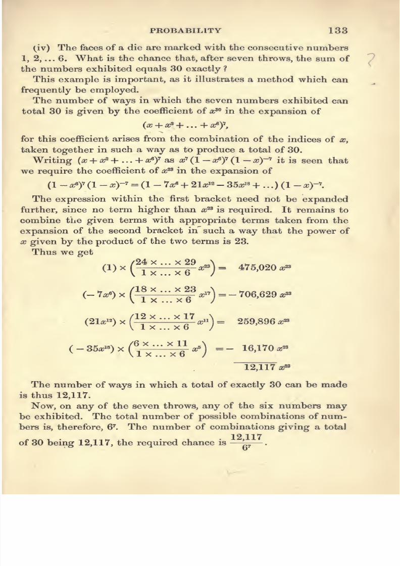
7/27/2019 7-CALCULUS AND PROBABILITY-1922-Alfred Henry.pdf
http://slidepdf.com/reader/full/7-calculus-and-probability-1922-alfred-henrypdf 147/170
PROBABILITY 133
(iv) The faces of a die are marked with the consecutive numbers
1, 2, ... 6. What is the chance that, after seven throws, the sum of
the numbers exhibited equals 30 exactly ?
This example is important, as it illustrates a method which can
frequently be employed.
The number of ways in which the seven numbers exhibited can
total 30 is given by the coefficient of a?^ in the expansion of
for this coefficient arises from the combination of the indices of a?,
taken together in such a way as to produce a total of 30.
Writing {x^-oc'+...+ af^J as x' (1 - a^y (1 - a;)-^ it is seen that
we require the coefficient of ar® in the expansion of
(1 -^y (1 -a?)-^ = (l - 7a;« + 21a^2_ 35^18+ ^^) (1 -x)-\
The expression within the first bracket need not be expanded
further, since no term higher than x ^ is required. It remains to
combine the given terms with appropriate terms taken from theexpansion of the second bracket in^ such a way that the power of
X given by the product of the two terms is 23.
Thus we get
/24X...X29 \^ 475,020 ar«^^\lx...x6 /
(« 7a;0 X f^f^'-^'f xA =-
706,629 aP^ ^ \ 1 X ... x6 /
12X...X17 „,259,896a;««
oi 12X/12X...X17 \
^'^ ^^>K ix...x6 n(-^bx'^)x(%^ '^^} A =- 16,170 a;«^ ^ \1 X ... X 6 /
12,117 a;»
The number of ways in which a total of exactly 30 can be made
is thus 12,117.
Now, on any of the seven throws, any of the six numbers may
be exhibited. The total number of possible combinations of num-
bers is, therefore, 6^ The number of combinations giving a total
12 117of 30 being 12,117, the required chance is
—^^
—

7/27/2019 7-CALCULUS AND PROBABILITY-1922-Alfred Henry.pdf
http://slidepdf.com/reader/full/7-calculus-and-probability-1922-alfred-henrypdf 148/170
134 PROBABILITY
15. The following miscellaneous examples are taken from the
examination papers of the Institute ; they illustrate various devices
which may be employed with advantage in the solution of questions
of this character.
(i) If n whole numbers be multiplied together, find the chance
that the last digit of the product is a five. [1910, Paper I, Q. 7.]
The chance is compounded of the separate chances that none of
the final digits of the n numbers is even and that one at least is a five.
The required chance is therefore
Kn _ 4,71
(j) i-a) }=-^.
(ii) Four coins are tossed together and A is to receive £2 if
exactly 2 heads turn up, and to pay £1 in any other event. Find
the probability that after four trials A is £1 out of pocket.
[1913, Paper I, Q. 8.]
To satisfy the conditions A must win once and lose thrice.
The chance that exactly 2 heads turn up equals the middle term
in the expansion of (^ + J)* = (^l ^ (i)* = i
Therefore the chance that he should win once and lose thrice
equals the second term in the expansion of (J + f)*, which is
4.|-(f)'=Tm-
(iii) If a coin be tossed 15 times, what is the probability of
getting heads exactly as many times in the first 10 throws as in
the last 5? [1915, Paper I, Q. 9.]
If n coins be tossed the chance that exactly r heads turn up
equals the (r + l)th term in the expansion of (^ -f J) .
Now in the last 5 throws we may get 0, 1, ... 5 heads and we have
to combine the chance of any of these with the chance of getting
the same number of heads in the first 10 throws. Thus we have
for the several chances of getting
heads in both sets of throws = {\f . {\Y
Ihead „ „ „ = 5(i)». 10(1^
2 heads
3 „
4 „
5 „
= io(iy. 45(iy°
=:10a)M20(iy<'
= 5(iy.210(i)-

7/27/2019 7-CALCULUS AND PROBABILITY-1922-Alfred Henry.pdf
http://slidepdf.com/reader/full/7-calculus-and-probability-1922-alfred-henrypdf 149/170
PROBABILITY 135
Therefore the total chance that the same number will turn up in
both sets of throws is the sum of each of these distinct probabilities,
. 3003
(iv) A and B throw for a certain stake, each throwing with one
die; ^'s die is marked 2, 3, 4, 5, 6, 7, and 5's 1, 2, 3, 4, 5, 6, and
equal throws divide the stake; prove that ^'s expectation is f|of
the stake.
What will J.'s expectation be if equal throws go for nothing?
[1911, Paper I, Q. 8.]
Let e equal ^'s expectation.
The chance of J.'s throwing any of the numbers marked on the
die is the same for each number.
If A throws Si. 2, B must throw a 1 if J. is to win the stake, or
a 2 if ^ is to divide the stake. The chance that A throws a 2 isJ;
the chance that he then wins the stake is ^ and that he divides the
stake is alsoJ.
His expectation if he throws a 2 is therefore J + J . i
If equal throws go for nothing, ^'s expectation after an equal
throw clearly remains at e. In that case his expectation if he throws
a 2 is J + Je.
We therefore have the following scheme:
A'8 throwChance ^'s expectation if equal ^'s expectation if equal
thereof throws divide the stake throws go for nothing
2 i+i-i i+i«3 i+i4 i+i^4 H*-4 i+*«5 §+*•* l+i«6 HJ-4 i+ie7 1 1
The total expectation being the sum of the separate expectations,
we have in the first case e = j^, being the sum of the figures in thethird column of the above table, and in the second case e =^ + ^e.
Whence e = ||.
(v) A man tosses 20 pennies and removes all that fall head up;
he then tosses the remainder and then removes all that fall head
up, and so on. How many times ought he to be allowed to repeat
this operation if he is to have an even chance of removing all the
pennies before he has finished? [1906, Paper I, Q. 11.]

7/27/2019 7-CALCULUS AND PROBABILITY-1922-Alfred Henry.pdf
http://slidepdf.com/reader/full/7-calculus-and-probability-1922-alfred-henrypdf 150/170
136 PROBABILITY
The problem is clearly the same if all the pennies are tossed
each time; we then have to find the chance that all the pennies
have turned up heads once at least
If n be the required number of throws, the chance that any
particular penny has turned up heads once at least is {1 — (J)**).
The chance that all the pennies have turned up heads once at
least is therefore {1 — (|) )^ and by the terms of the question this
must equalJ.
Solving this equation we find (1)** = 1 — (J)^,
n = 4-87.-n
(vi) 2** players of equal skill enter for a tournament; they are
drawn in pairs, and the winners of each round are drawn again for
the next. Find the probability that two given competitors will play
against each other in the course of the tournament. If w = 5, show
that the probability that a given player will either win or be
beaten by the actual winner is ^. [1912, Paper I, Q. 6.]
As regards the first part of the question, the total number of
games that will be played is
2n-i^_2»-2+ ...+1=2'»-1.
2** (2^ — 1)Also two players can be selected in ^ ways. The chance
that two will meet is therefore the quotient of these two values,
1
^•^•2^1-
The second part of the question can be proved by an inductive
process.
Let Un be the required chance.
Then in the first round he may either win or lose. If he wins,
he passes into the next round and his chance of winning or being
beaten by the ultimate winner then becomes Wn-i- If he loses, his
opponent passes into the next round where the latter's chance of
becoming the ultimate winner is increased to ^^^ .
We thus have
2 **-' ^ 2 2'^^n — n ^n—1
+ o•
Qn-l

7/27/2019 7-CALCULUS AND PROBABILITY-1922-Alfred Henry.pdf
http://slidepdf.com/reader/full/7-calculus-and-probability-1922-alfred-henrypdf 151/170
Similarly
PROBABILITY
1
2
1
»l~2 + ^•
1
2n-2 '
1
41
. 1 1
2n-3'
etc. etc.
1
2n-
1
t^ + 2^:
1
-^•2*
137
As t^ obviously equals 1, we have by addition
1 n-1 n+1'^ <2n-\
^ 2^n =2»
^5 = A.
It is instructive also to prove the first part of the question
inductively.
Let Un be the required chance. This chance is compounded of
the two chances that they meet in the first round, or that, nothaving met in the first round, they both pass into the second
round where the corresponding chance becomes Wn-i-
The chance that they meet in the first round is -^—=- ; the chance
2'* — 2that they do not meet is^—r-
. Therefore we have
1 1 2 -2^«-2 -l'^^'^'*4*2»~l'
or (2'* - 1) i*^ = 1 + ~ Un-i.
C2 ~i— 1 1
2 )^n-i = 2+
2»-2 _ 1
4^n-2
.2n-2^\ _1 2^-^ - 1
\~ir~)^'^^
- 4 ^
8^'*-
etc. etc,
/2» - \ _ _1_ 2^-1
\2 ~^ y
'^3 — 2n-3'^ ~2n=r^2'
/22-l\ __ 1 2-1
\

7/27/2019 7-CALCULUS AND PROBABILITY-1922-Alfred Henry.pdf
http://slidepdf.com/reader/full/7-calculus-and-probability-1922-alfred-henrypdf 152/170

7/27/2019 7-CALCULUS AND PROBABILITY-1922-Alfred Henry.pdf
http://slidepdf.com/reader/full/7-calculus-and-probability-1922-alfred-henrypdf 153/170
EXAMPLES
CHAPTER III
1. Given
/(l)= (^-2)(^-3), f{^) = {x-l){x-b), /(3)= (^-10)(:r+ l), /(4)= 63,
obtain a value for x^ assuming second diflFerences are constant.
2. Find the nth term of the series 2, 12, 36, 98, 270, 768, etc. and the sum
of n terms of it.
3. Given that
/(0)= 66566, /(1)= 65152, /(2)= 63677, /(3)= 62136,
find/(9).
4 Find A-' ^^+2^
(3^ + l)(3a;+4)(3^^ + 7)(3^+10)
5. Find the value of
A (3^+ 1) (3^+4) (3;r+ 7) ... (3^+ 3?i-2).
6. Prove that
2i
+ ...+/ (:r+ m)= 7^'»/ (^)+ wTi* - A/ {x)
+^'^ffi^w™-2Ay(^)+ ... + A »/(^).
Hence find the sum of the series
l2+m.22+^?^i|pD32+ ... + (7/i+ l)2.
CHAPTER IV1. Given
/(0) = 70795, /(1)= 72444, /(2)= 74131, and /(6)= 81283,
find /(3),/(4), and /(5).
2. Find/ (35) given
/(20)= '01313, /(30)= -01727, /(40)= -02392, / (50)
= -03493.
3. Supply the missing term in the following table
/(0)= 72795,
/(1)= 71651,
/ (2)= 70458,
/ (4)=67919,
/ (5)= 66566,
/(6) = 65152.
4. Given
/(0)= 11, /(3)= 18, /(6)= 74, and/(9)= 522,
find the intermediate terms.

7/27/2019 7-CALCULUS AND PROBABILITY-1922-Alfred Henry.pdf
http://slidepdf.com/reader/full/7-calculus-and-probability-1922-alfred-henrypdf 154/170
140 EXAMPLES
.5. Given
/(0)=98203, /(1)= 97843, /(2)= 97459, /(3)=97034,
find/ (2-25).
6. Given
/(0)= 98023, /(10)= 97651, /(20)= 97246, /(30)= 96802,
find/(15).
7. Given
/(0)= 58'842, /(2)= 55-267, /(4)=51-368, /(10)= 37-977,
complete the series /(O), /(I), .../(lO).
8. If you were asked at very short notice to obtain approximate values for
the complete series /(O), /(I), /(2), .../(20), being given that /(0)= -0I3,
/(10)=-248, /(15)= -578, and /(20)= -983, what methods would you adopt,
and what value would you obtain for/(9)?
9. /(1)=1; /(2)+/(3)= 5-41; /(4)+/(5) 4-/(6) = 18-47;
/(7)+/(8)4-/(9)+/(10)+/(ll)+/(12)=90-36.
Find the value of/(^) for all values of x from 1 to 12 inclusive.
10. Apply Lagrange's formula tofind/ (5) and/(6), given that
/(1)= 2, /(2)= 4, /(3)= 8, /(4)= 16and/(7)= 128;
and explain why the results differ from those obtained by completing the series
of powers of 2.
11. Find the simplest algebraic expression in x which has the values 5, 3,
9, 47 and 165 when x has the values 0, 1, 2, 3 and 4 respectively.
12. Prove the following formulas for approximate interpolation
/(l)=/(3)-3[/(5)-/(-3)]+-2[/(-3)-/(-5)](1),
/(O) =i [/(I) +/(-l)]-|[H/(3) -/(I)} -i {/(- )-/(- 3)}] ...(2),
and apply them to find the logs of 45, 46, 47, 48, 49, being given
log 42= 1 -62325, log 50= 1 -69897,
log 44=1-64345, log 52= 1-71600.
13. Given
10 10 10
2/(^)= 500426, 2/(^)= 329240, 2/(^)= 175212 and /( 10)= 40365,
147
find/(l).
CHAPTER V
1. Use Gauss' interpolation formula to obtain the value of/ (41) given
/(30)= 3678-2, /(35) = 2995-l, /(40)= 2400-l,
/(45)= 1876-2, /(50) = 1416-3.
Verify your result by using Lagrange's formula over the same figures.

7/27/2019 7-CALCULUS AND PROBABILITY-1922-Alfred Henry.pdf
http://slidepdf.com/reader/full/7-calculus-and-probability-1922-alfred-henrypdf 155/170
EXAMPLES 141
2. Given the following table find/(28) using Stirling's formula:
/(20)= 98450, /(25)= 96632, /(30) = 94472,
/(35)= 91852, /(40)= 88613.
3. Prove that
/(x)=4[/(-i)4./(4)]+x./(-4)+-±^i.4y(^?)+AyU)+....
and apply the formula to find/ (32) given
/(25)=-2707, /(30)= -3027, /(35)= -3386, /(40)= -3794
4. From the table of annual net premiums given below find the annual net
premium at age 25 by means of Bessel's formula
Ago Annual Net Premiums
20 -01427
24 -01581
28 -01772
32 -01996
5. Use Everett's interpolation formula to complete the series /(25) to /(35),
given that
/(15)= 305, /(20)=457, /(25)= 568, /(30)= 671,
/(35) = 897, /(40) = 1190, /(45)= 1481.
CHAPTER VI
1. Given the following table oif{pc) :
/(0)=217, /(1) = 140, /(2)= 23, /(3)=-6,.
show how to find approximately the value of cs for which the function is zero.
2. Given that, when
^=0, /(:r)=0,
^=1, /(^) = 100,
x= 2, /(a?)= 2000,
find X when /(^)=1900 by Lagrange's formula of interpolation (applied
inversely) and explain why the result does not agree with that found by using
the formula/(:j7)= (l + A)*/(0) and solving the quadratic
3. The following values of/(a?) are given
/(10)= 1754, /(15)=2648, /(20)=3564.
Find, correct to one decimal place, the value of x for which /(a:)= 3000.
4. /(30)=-30, /(34)=-13, /(38) = 3, /(42)= 18.
Apply Lagrange's formula of interpolation inversely tofind x^ where /(a;) =0.

7/27/2019 7-CALCULUS AND PROBABILITY-1922-Alfred Henry.pdf
http://slidepdf.com/reader/full/7-calculus-and-probability-1922-alfred-henrypdf 156/170
142 EXAMPLES
CHAPTER VII
1. Find the value of
A- L7i (?i+ l) (rH-2) ... (7i+r- 1)
and use the result to find the value of
2^(^ + 1) (^+ 2)'
2. Prove that
1
3. Show that
where ^ (a?) is any rational integral algebraic function of x.
4. Prove that if a„ diminishes as n increases and converges to the limit zero,
the sum to infinity of the series ai — ag+as ... is the same as the sum to infinity
of the series iai — lAa^+^A^a^ - etc.
Find the sum to infinity of the series ^-^+^ .- true to four decimalplaces.
5. Prove that if the fourth and higher differences are ignored the sum of n
successive terms of a function of which /(O) is the central term is
/w+^^'/^-i)'
where n is an odd number.
CHAPTER VIII
1. Given the following values oif{x):
/(I •41)=
-7092, /(l-49)= -6711,
/(I -62)= -6579, /(l-53)= -6536,
find/(l-45).
2. Use Divided Difierences to find/ (80) to the nearest integer, given
/(70)= 235, /(71)= 256, /(79)=436, /(81)= 484.
3. Given
/(20)= -342, /(23)= -391, /(31)= -516, /(34) = -559,
find/(30) by means of Divided Difierences, and check the result by applying
Lagrange's interpolation formula.

7/27/2019 7-CALCULUS AND PROBABILITY-1922-Alfred Henry.pdf
http://slidepdf.com/reader/full/7-calculus-and-probability-1922-alfred-henrypdf 157/170
EXAMPLES 143
CHAPTER IX
1. The following values of/(^, y) are given
/ (35, 55)= 10-020, /(35, 50) = iri96, /(35, 45) = 12-019,
/(40, 55)= 9-796, / (40, 50)= 10-894, / (40, 45) = 11-641,
/(45, 55)= 9-583, /(45, 50)= 10-591, / (45, 45)= 11-243.
(i) Using only six of the above values, find/(42, 52).
(ii) Making use of all the data calculate/(44, 51).
2. Prove that if/(O, 1)=/(1, 0) and/(0, 2)=/(2, 0), then
/(^, 3')=/(0,0)+ (^+y)[A,+^±|::^A2,J/(0, OHxy[f{l, l)-/(2, 0)].
Find/ (39, 33), given
/(35, 35)= 3-151, /(35, 45)=3-912,
/(35, 40) =3-471, / (40, 40)= 3-766.
CHAPTER XI1
1. Find the differential coefficients with regard to x of log^« and
\/^2_3
(^-l)\/^2_7
2. Differentiate with respect to x
^^
Va^+ ax+x'^
•
3. Find the differential coefficient with regard to x ^ of
4. Differentiate
(1) «;« f -J
log -, with respect[to log -
,
x^(2) log——r , with respect to a?,
(3)^Ooga;)2, ^j^j^ respect to x.
5. If(l-a?)v+(l-y)^=0, find^,
6. Obtain the differential coefficients of
X
a*
1) ^^§5' (2) e^» with respect to x.

7/27/2019 7-CALCULUS AND PROBABILITY-1922-Alfred Henry.pdf
http://slidepdf.com/reader/full/7-calculus-and-probability-1922-alfred-henrypdf 158/170
144 EXAMPLES
CHAPTER XII
1. Find (1) the nth. differential coeflQcient of -—jrj~2—Tn
^*^ respect to
a:, and (2) the second differential coefficient of log^ (1 -\-x) with respect to log^ x.
2. Find the nth differential coefficient ofe^{x- 2)2.
3. Having given that
provethat a:^^,M2n+l) a:, ^^^n'^1)^^= 0.
4. Obtain the second differential coefficient of log {a-\-bx+ cx^) with respect
to -Jx.
5. Find the Tith differential coefficient with respect to ^ of
x+\2^2_5^^.3-
CHAPTER XIII
1. Provethat ^=i_^ + ^_^...e*-l 2 12 720
and show that no odd power of x beyond the first can occur.
o 15 ^v, ^.log(^+\/l+ ar2) 2.4 ,
2. Provethat ^^,
—x-la^+ ^i—,x^-,„.s/\+x^ ^ 3.5
3. Prove that the first three terms of the expansion of {\-\-xY in powers of
X are e - — + ^J ex ^.
4. Expand log {x+ Va^ ^ ^2) \ji ascending powers of x.
6. Expand —^—-—' in ascending powers of x as far as the term in-
volving a^.
CHAPTER XIV
2. Find the maximum value oi x{x-\){x-'i) between the limits and 1.
3. Find the values of x at the points where the graph of the function
(1 +a?2) e^-** has its greatest slope.

7/27/2019 7-CALCULUS AND PROBABILITY-1922-Alfred Henry.pdf
http://slidepdf.com/reader/full/7-calculus-and-probability-1922-alfred-henrypdf 159/170
EXAMPLES 145
4. A man in a boat at sea, 5 miles distant from the nearest point of a
straight shore, wishes to reach a place 12 miles distant along the shore,
measuring from this nearest point. At what point should he land to reach this
place in the minimum time, if he can row at 3 miles an hour and walk at4 miles an hour?
5. Given/(0) = 1876,/(1)= 777,/(3) = 19, and/(6)= -218, interpolate the
values of /(2), /(4), and /(5) and i&nd the values of x for which f{x) is a
maximum or minimum.
6. Find the minimum and maximum values of
x^-^- %x^+ 48^ - 48.
7. A window is in shape a rectangle with a semicircle covering the top. If
the perimeter of the window be a fixed length l^ find what is its maximum area.
8. Fmd (1) Lt .,
(2) Lt(l+a,'3)^.a;-*-o
CHAPTER XVd^ fix)
1. Show that -^-—^=Ay(:r-f) approximately.
By considering the function f{x)— a+ hx-{-cF and using the above relation
prove that logeC=c*-c~* approximately, where c is a small quantity.
A2 a32. Show that aO *- — 0* + — 0 » ...=0, when m > 1.
2i S
3. Prove that, if f{x) be a function the fourth differences of which are
constant,
'^£-^=l^[/(^-2)-8/(^-l)-f8/(^+l)-/(^+2)]
and hence find an approximate value for -r- flog /(a?)] where
/(^- 2)= 42-699, /(^-1)= 40-365, /(a?)=37-977,
/(^ + 1) =35-543, /(a;+ 2)= 33-075.
CHAPTER XVIII
1. Find the integrals
(^)/Jh<'- ^^)/^ ^- («)f-^^^-
jx*a*dx.. Evaluate
H. T. B. I. 10

7/27/2019 7-CALCULUS AND PROBABILITY-1922-Alfred Henry.pdf
http://slidepdf.com/reader/full/7-calculus-and-probability-1922-alfred-henrypdf 160/170
146 EXAMPLES
3. Evaluate
„. , .. . . r27a?2- 171^+256 ,
Find the value of I -z-. ^^^-t——rr- dx.
Liate
4.
5. Evaluate
CHAPTER XIX
1. If /(^)=a+J^+ca;2, find expressions for /(J),-=^^ and / f{x)dx in
terms of/(0),/(l) and/(2).
2. Evaluate ^.^^dx.
3. Find the value of P-^^^t^J^^rf^P.;j j7(2-a:)(a7+l) ^
4. Find the average value of x {x—l){x-2) between the limits and 1.
5. Find the value of / x^^'-^e^dx.
CHAPTER XX1. From the table
/(0)= 217, /(1)= 140, /(2)«=23, /(3)=~6,
find an approximate value for / f(x) dx, and explain why the result difiers
from/(0)+/(l)+/(2)+/(3).
2. Prove that approximately
J;^^/(^)rf^=2V{/(-l)+22/(0)+/(l)},
and find thereby an approximate value for
r* 10,000 X 4-* x23'ffx
3. Discuss the error in assuming that
JV(^)^^=/(4)=M/(0)+/(i)]
if (1) f{x)=a+bx+cx^, (2) /(^)=100x4*
4. Given /( - 2), /(O), /(2), find an approximate value for
j[j(x):dx.

7/27/2019 7-CALCULUS AND PROBABILITY-1922-Alfred Henry.pdf
http://slidepdf.com/reader/full/7-calculus-and-probability-1922-alfred-henrypdf 161/170
EXAMPLES 147
5. Prove that
1
/;f{x)dx=^ [5/(1) + 8/(0) -/(-I)] approximately.
If the speed of a train on a non-stop run is as shown in the table below, find
the approximate mileage travelled between 12.0 and 12.30, using the above
formula.
TimeSpeed in
miles per hour
11.50
12.0
12.1012.20
12.30
24-2
35
41-342-8
39-2
6. If/(1)= 4157, /(2) = 4527, /(4)= 6435, find approximately the value of
/:f{x) dx.
CHAPTER XXI
1. n persons are sitting at a round table, and from them three are selected
at random ; show that the chance that no two of those selected are sitting next
one another is, r^r -J: .
(7l-l)(?l-2)
2. A heap of playing cards contains 6 hearts, 5 spades and 4 clubs. A card is
chosen at random 9 times in succession and is not replaced. Find the chance
(1) that there are no hearts left, and (2) only hearts are left.
3. A man has two sovereigns and four shillings in his pocket ; from these
he selects at random 3 coins, and again chooses from these 3 coins at random,
the first coin for A^ the second for i5, and the third for C.
Find the values of the expectations of J[, 5, and G.
4. Find the probability that out of 5 persons aged 45 exactly 3 will die in
a year.
Probability that a person aged 45 will die in a year= '01224.
5. A die with six faces is thrown three times and the sum of the throws is
twelve : find the chance (1) that the first throw was a four : (2) that four was
thrown each time.
6. Two men, A and B^ each draw a card from a well-shuffled pack of
playing cards, find that they are of the same value, and replace the cards
they do this four times in succession. Find the chance that this would happen
andshow
that it is
approximately ^^.
\f

7/27/2019 7-CALCULUS AND PROBABILITY-1922-Alfred Henry.pdf
http://slidepdf.com/reader/full/7-calculus-and-probability-1922-alfred-henrypdf 162/170
148 EXAMPLES
7. The probability that a man aged 50 will survive one year is •98428.
Show that the probability that, out of 5 men aged 50, 3 at least will die within
a year is -0000385.
8. The 26 letters of the alphabet are placed in a bag. A and B alternately
draw a letter from the bag, the letters drawn not being replaced. The winner
is the one who draws most vowels. A starts and draws a vowel with his first
draw. What is his chance of winning ?
9. If a number of five figures containing any five of the ten digits once only
is written down at random, what is the probability that it is divisible by 9 ?
10. Given the following table find the probability that one at least of three
persons aged respectively 20, 30, 40 will die between the 10th and 20th yearfrom now
Age
Probability
of surviving
10 years
Probability
of surviving
20 years
20
30
40
•93363
•91740
•88476
•85651
•81167
•71517
X
11. Two persons, A and 5, play for a stake, each throwing alternately two
dice, A commencing. A wins if he throws six, B if he throws seven, the game
ceasing as soon as either event happens. What ratio will ^'s chance of winning
bear to i?'s?
12. The sum of two positive integers (excluding zero) is 100 j find the chance
that their product exceeds 1200.
13. The following table shows the probability that a woman of the age
specified will marry in a year
Age Probability of marriage
20 -0665
25 1033
30 ^0649
40 -0183
Find the probability that, out of 4 women aged 20, 25, 30, 40 respectively, only
one marries within a year.
14. A bag contains 8 counters, numbered 1 to 8. Four are drawn at
random. Find the chances that
(1) The sum of the numbers on the foiu* counters amounts to at least 17.
(2) The counters numbered 2 and 3 are among the four.
(3) The four counters contain at least two of the three counters numbered
3, 5 and 7.
15. A penny is tossed six times. Find the chance that neither heads nor
tails have occurred three times in succession.

7/27/2019 7-CALCULUS AND PROBABILITY-1922-Alfred Henry.pdf
http://slidepdf.com/reader/full/7-calculus-and-probability-1922-alfred-henrypdf 163/170
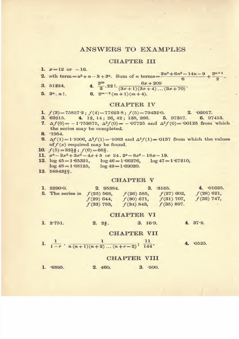
7/27/2019 7-CALCULUS AND PROBABILITY-1922-Alfred Henry.pdf
http://slidepdf.com/reader/full/7-calculus-and-probability-1922-alfred-henrypdf 164/170
ANSWEES TO EXAMPLES
CHAPTER III
1. x=l2 or -16.
2. 7«th term=7i2+n- 3+ 3 . Sum of n terms= ^ '^~9~
3. 51224. 4. ?.22 .^^^^^^
2 (3a:+ l)(3:c+ 4)...(3a?+ 70)
5. 3 .7i . 6. 2^-2(m + l)(w + 4).
CHAPTER IV
1. /(3)= 75857-2 ;/(4)= 77623-8 ;/(5)= 79432-0. 2. -02017.
3. 69215. 4. 12, 14 ; 26, 42 ; 138, 266. 5. 97357. 6. 97453.
7. A/(0)= -1-753875, Ay(0)=- 07725 and a3/(0)= -00125 from which
the series may be completed.
8. -1954.
9. A/(l) = l-1006, a2/(1) = -1083 and A3/(l)r=-0137 from which the values
off{x) required may be found.
10. /(5) = 32H;/(6)= 66§.
11. a;4-2a:3+ 3x2-4a: + 5 or 24. 2*-8^2_i8a;_i9.
12. log 45= 1-65321, log 46= 1-66276, log 47= 1-67210,
log 48= 1-68125, log 49= 1-69020.
13. 58843|f.
CHAPTER V
1. 2290-0. 2. 95384. 3. -3165. 4. -01625.
5. The series is / (25) 568, /(26) 585, /(27) 602, /(28) 621,
/(29) 644, /(30) 671, /(31) 707, /(32) 747,
/(33)793, /(34)843, / (35) 897.
CHAPTER VI
1. 2-751. 2. 2jf. 3. 16-9. 4. 372.
CHAPTER VII
1. JL. I . IL. 4. 0525.
l-r n{n+ l){n+ 2)...{n+r'-2)' 144'
CHAPTER VIII
1. -6895. 2. 460. 3. '500.

7/27/2019 7-CALCULUS AND PROBABILITY-1922-Alfred Henry.pdf
http://slidepdf.com/reader/full/7-calculus-and-probability-1922-alfred-henrypdf 165/170
ANSWERS TO EXAMPLES 151
CHAPTER IX
1. (i) 10-389; (ii) 10-475. 2. 3-297.
CHAPTER XI
1- xr2(l-log^)^ (a;-l)2(^2_3)i(^2_7)f
2x^C^a^+^ax+x^)
^1
• 3{a+ x){a^+ x^){a^'{-ax+x-^)' '
a^ ^^^Z^'
4. (1) a=«(^) [:rloga.log^+a^log^(log^ + l) +lJ,
, . 1__
1 3^(108^)' (log ^)2
«•-^ ;:5::::g:gSg:S - «• ^'-^ ^-(--^)-
CHAPTER XII
1 m (-1) -^^ 1 1 2(7^+1) 1 .g. ^logg^•^^
4L(^-l)«
+ i (^
+l)'» + i (^
+ l)
+ 2j> ^^^
(l + a;)2-
2. e«=«.a -2[a2(^_2)2+ 2m(a?-2) + 9i(7i-l)].
. [a6+ ^ (6ca- 52) - hcx'^ - 20^^^]
5 (-i)n ^jf5-2^ 2 n
^'^ ^^
•''•L(2^-3)«+ i (a?-l)« + ij-
CHAPTER XIII
A 1 4.^_^4.^_ ,/ ,,, 1.3...(2r-l)a;2r-n ^
4. ioga+ ^ 6a3'* 40a6 • ^^ ^ r (2r+ l)2»-a2'-+i
^••••
_ a?2 5^ a;^ 209^^' ^ 2~12 ^4+'720~-
CHAPTER XIV
2 /^ 151. 1. 2. Tz . 3. + A. /-. 4. —7= miles from the nearest point
3 73-
V2
775. /(2)= 218, /(4)=0, /(5)= -19. _
120+\/llOMaximum value when x
Minimum value when x=
30
120-\/riO
30
6. Minimum values- 3, - 128. Maximum value 0.
El
2(7r + 4)
7. TTT^ ..> 8. (1)
x/f^'^5(^^ ^-

7/27/2019 7-CALCULUS AND PROBABILITY-1922-Alfred Henry.pdf
http://slidepdf.com/reader/full/7-calculus-and-probability-1922-alfred-henrypdf 166/170
152 ANSWERS TO EXAMPLES
CHAPTER XV3. -06353.
CHAPTER XVIII
1. (1)
2_^^l(5^+6.2+8.+16) + c; (2) ^^3 log(^^+ c
(3) log^[log(log^)-l]+c.
Lloge« (log.a)2'* (logea)3 (log,a)4 ̂ (log,a)0+''-
3. (1) ^ [{x+ ct) \/ar2+ 2ax- a^ log {(^ -\-a) + fjx'^+ 2aa;} + c]
(2) H«'-^)'-«V^=^+c; (3) ''^^^\o^{\^x)^c.
- x-%,-. a?-3.
5. log(f^) +^ + ^; (l+a;)log(l+^)-(l-^)log(l-^)-2a?+c;
j^-|-j^[{(7i + l)log2r)3-3{(w+l)log^}2+ 6(n+l)log:r-6] + c.
CHAPTER XIX
1. i[3/(0) + 6/(l)-/(2)];i[-3/(0)+4/(l)-/(2)];
^[6/(0) + 8/(l)-/(2)].
2. ^. 3. log,6. 4. i. 5. ^.
CHAPTER XX1. 262^. 2. 32500. 3. (1) -Jjc; Jc. (2) -16*5; 33*5.
4. I [3/(- 2)+ 2/(0)+ 3/(2)]. 5. 20 '4 miles. 6. 14262.
CHAPTER XXI
2. (1)7^; (2) F?^. 3. 75. 4rf., 75. 4c;., 7«. 4fl?. 4. -0000179.
5. (1) \\ (2) ^. 6. ^h^. 8. i^,9. i. 10. -31466. 11. 30:31. 12. 1%.
13. -2109. 14. (l)|f; (2)^; (3) i. 15. M-16. (1) f; (2) tI&5. 17. ^'s chance Iff|§; 5's chance ^0^.
21. e|. 22. §-ilog3.
CAMBBIDGB : PRINTED BY J. B. PEACE, M.A., AT THE UNIVEBSITY PRESS.

7/27/2019 7-CALCULUS AND PROBABILITY-1922-Alfred Henry.pdf
http://slidepdf.com/reader/full/7-calculus-and-probability-1922-alfred-henrypdf 167/170

7/27/2019 7-CALCULUS AND PROBABILITY-1922-Alfred Henry.pdf
http://slidepdf.com/reader/full/7-calculus-and-probability-1922-alfred-henrypdf 168/170

7/27/2019 7-CALCULUS AND PROBABILITY-1922-Alfred Henry.pdf
http://slidepdf.com/reader/full/7-calculus-and-probability-1922-alfred-henrypdf 169/170
f^.Bl)24G
af\43l
H3
UNIVERSITY OF CALIFORNIA LIBRARY
em^~.^^
'^^^Mm

7/27/2019 7-CALCULUS AND PROBABILITY-1922-Alfred Henry.pdf
http://slidepdf.com/reader/full/7-calculus-and-probability-1922-alfred-henrypdf 170/170