7 7 -AIBI 763 A AN I IES C ILYTEJCHNIGIIE 1/3

UNCLASSIFE A QEcSE AL.19 l98AFSN 99-6 F/G 13/7 ML

1.0 LM'I36

1 Io

r7rW

'7'-

S'17

V-7-v, --Y'

tellA

77

jOo nift-st-Am

OOW v

Prii"011114111146". C wan

A I A" doigo OWWWW Of

hdoom des tur-

7 ", T7-L116-

COMMUNICATIONDU LABORATOIRE DE THERMIQUE APPLIQUEE ET DE TURBOMACHINES

DE L'tCOLE POLYTECHNIQUE FEDERALE DE LAUSANNEPROF. DR. A. BOLCS

____ ____ ___ ____ ____ ___ Nr. 13

AEROELASTICITY IN TURBOMACHINESCOMPARISON OF THEORETICAL

AND EXPERIMENTAL CASCADE RESULTS

par

DR. A. BOLCS ET DR. T.H. FRANSSON 7

Cii o rE

Lists

LAUSANNE, EPFL F1986-

__.;__ ___ ___

UNCLASSIFIED "SECURITY CL-It rO THISP7AG

REPORT DOCUMENTATION PAGEIa. REPORT SECURITY CLASSIFICATION lb. RESTRICTIVE MARKINGSUnclassified

2. SECURITY CLASSIFICATION AUTHORITY 3 DISTRIBUTION/AVAILABIUTY OF REPORT2b. DECLASSIWICATION/OWNGRADING SCHEDULE Approved for public release;

Distribution unlimited

.PERFORMING ORGANIZATION REPORT NUMBER(S) S. MONITORING ORGANIZATION REPORT NUMBER(S)

i. NAME OF PERFORMING ORGANIZATION [6b OFFICE SYMBOL 7a. NAME OF MONITORING ORGANIZATIONEcole Polytechnique Federale dej (f plicable) European Office of Aerospace R.esearch andLausanne I Development

V_ #MSS (am r ' ande) 7b ADDRESS (City, State, and ZP Code)Laooratolre ae thermique Appliquee et de Box 14

Turbomachines F"O New York 09510-0200CH-1015 Lausanne, Switzerland

Be. NAME OF FUNDING/SPONSORING Sb. OFFICE SYMBOL 9. PROCUREMENT INSTRUMENT IDENTIFICATION NUMBERORGANIZATION Air Force Office (If 99Lkablk) AFOSR 84-0105of Scientific Research I NA

87 E , andIPC10. SOURCE OF FUNDING NUMBERS

0iPROGRAM I RJC AK IWORK UNITBoiling AFB, DC 20332-6448 ELEMENT NO. I No. No ACCESSION NO

61102F I 2307 I Bl

1It. TITLE fticlud" Aewfty C/lssiifical~o)AEROELASTICITY IN TURBOMACHINES

COMPARISON OF THEORETICAL AND EXPERIMENTAL CASCADE RESULTS

12. PERSONAL AUTHOR(S) Dr. A. B8lcs and Dr. T. H. Fransson

13.. TYPE OF REPORT 13b. TIME COVERED 114. DATE OF REPORT (Year, Month, Day) rS. PAGE COUNTFinal Scientific I FROM 2 May 84

"O 1 Nov85 1986

16. SUPPLEMENTARY NOTATION

17. COSATI CODES 1B. SUBJECT TERMS (Continue on revere if necesary and identify by block number)FIELD GROUP SUB-GROUP Aeroelasticity Flutter

Turbomachinery Cascade Flow

.ABSTRACT (Continue on reverse if necessary and identify by block number)The aeroelastician needs reliable, efficient methods for calculating unsteady blade fcrces inturbomachines. The validity of such theoretical or empirical prediction models can be estab-lished only if researchers apply their flutter and forced vibration predictions to a number ofjwell documented experimental test cases.In the present report, the geometrical and time-averaged flow conditions of nine two-dimen-sional and quasi-three-dimensional experimental (mainly) standard configurations for aero-elasticity in turbomachine-cascades are given. Some aeroelastic test cases are defined foreach configuration, comprising different incidence angles, Mach numbers, interblade phaseangle, reduced frequencies, etc.Furthermore, a proposal for uniform nomenclature and reporting formats is included, in orderto facilitate the comparison of different experimental data and theoretical results.In total, results from 15 theoretical prediction methods have been compared with each other,and with experimental data. (continued on reverse side)

20. DISTRIBUTION i AVAILABIUTY OF ABSTRACT 21. ABSTRACT SECURITY CLASSIFICATIONIUCASSIFIEDAUNUMITED 03 SAME AS RPT. 03 DTIC USERS Unclassified

22a. NAME OF RESPONSIBLE INDIVIDUAL 22b. TELEPHONE (Includ Atea Code) Z Kc. OFFICE SYMBOLDR. ANTHONY AMOS (202) 767-4937 AFOSR/NA

DO FORM 1473,4 MAN 83 APR edition may be used until exhausted. SECURITY CLASSIFICATION OF THIS PAGEAll other editions are obsolete. UNCLASSIFIED

N' ,I" . :,

Item 19 (continued)

The comparative investigation has shown that present theoretical models can predict accuratelythe aeroelastic behavior of certain cascade configurations in two-dimensional flow. Otherconfigurations, on the other hand, cannot be predicted as well.It is concluded that, although present methods can predict stability limits in some cases,the physical reasons for flutter in cascades are not yet fully understood. Further investiga-tions, both experimental and theoretical, are thus urgently required.

AEROELASTICITY IN TURBOIIACHINES

COIPAEISOU OF THEORETICAL AND EXPERIFENTAL CASCADE RESULTS

Editors: A. 86tca and T. Fraosson

June 30, 1956This study Is sponsored jointly by the United States Air Force under GRANTSAFOSR 51-0251, AFOSR (13-0063, AFOSR 04-0105 with Dr. Anthony Amos asprogram manager, and by the Swiss Federal Institute of Technology, Lausanne.

Communication de Laboratoirs de Thernlique Appliquie et do TurbomachinesN413, 19MEcols Polytechnique Fdrale do Lausanne, Switzerland.

(PV-LAWum.. LAORATOIRE DE THERMOIUE APPLIQUEE ET DE TURBOMACHINES 2

AEROELASTICITY IN TURSOIMACIINES: Preface. Nomenclature 3

I. Pref ace

At the 1980 *Symposium on Aeroelasticity in Turbomachines 1I-31, held inLausanne, Switzerland I, it became clear that It was virtually impossible tocompare different analytical models for predicting flutter and forcedvibration and establish their validity.The Scientific Committee2 of this meeting decided to initiate a workshop on'Standard Configurations for Aeroelasticity in Turbomachine-Cascades'. Theaim of this project is to establish a data base with some well documentedexperimental data, and to initiate and coordinate future experimentalinvestigations in existing test facilities. The standard configurations to becompiled should also serve as test cases for present and future models forpredicting aeroelastic phenomena in turbomachine-cascaJes. It was decided bythe Scientific Committee that this study should be coordinated by the

"Laboratoire de thermique appliqude et de turbomachines" at the EPF-Lausanne, and that Mr. T. Fransson should undertake the task under an UnitedStates Air Force Contract.A first report with a set of standard configurations was distributed to all theparticipants at the end of 1983 [413. Calculations were subsequently

1 Three symposia have been held in this sere (Paris, France 1976;

Lausanne, Switzerland 1980; Cambridge, UK 1964) and a fourth is scheduledfor 1987 (Aachen, West Germany).

2 Scientific Committee:

Germany - H. F6rschingSwitzerland A. B61cs (P. Suter 1980. G. Gyarmathy 1976, 1980)France E. Szechenyi (R. Legendre, M. Roy 1976, 1980)UK D.S. Whitehead (+ J.E. Ffowcs Williams, D.G.M. Davis,

RJ. Hill 1984)Japan Y. TanidaUSA M. F. Platzer (+ M.E. Goldstein 1984, A.A. Mlkolajczak

1980)

3 Please note that, at the request of some participants, a few symbolsand standard configurations in the present report do not correspond to thosein Ref. 4. Refer to the section entitled "Updating of Nomenclature' for thesechanges.

.1 2.,:

EPF-Leusanne, LABORATOIRE DE THERMIQUE APPLIQUE ET DE TURBOMACHINES 4

performed and comparisons between experimental data and theoretical resultswere presented at the Third Symposium (1984) [71. The conclusion drawn fromthe work was promising and it was decided to continue the comparativeefforts, while encouraging new experimental and theoretical investigations,until the Fourth Symposium (1987).Special emphasis should now be put on defining a small set of aeroelastictest cases for detailed comparison between experiments and theories, tocoordinate new investigations and to discuss the physical phenomena ofaeroelasticity.The objective of the present report is to conclude the workshop initiated in1980, and look ahead to the Aachen Symposium, by which time the methods sovalidated may be used for detailed and systematic calculations, In order toobtain a better understanding of the aeroelastic phenomena.This exercise should serve as a guideline for the improving the numericalmodeling that will be required to achieve the goal of providing an efficientand reliable unsteady aerodynamic analyses, which can be used inturbomachinery aeroelastic design investigations 15).The Scientific Committee hopes that this report will constitute a bench-mark for the validation of both experimental and theoretical aeroelasticinvestigations in turbomachines.The present report will be updated at the Aachen Symposium, so that any new

experimental and/or theoretical investigations can be included.The members of the Scientific Committee express their thanks to Mr. T.Fransson, who coordinated, compiled and evaluated all the results, and to allresearch colleagues who participated in the study.For the Scientific Committee

A B6cs

AL-

AEROELASTICITY IN TURBOMACHINES: Preface. Nomenclature 5

II. Abstract

The aeroelastician needs reliable, efficient methods for calculatinq unsteadyblade forces in turbomachines. The validity of such theoretical or empiricalprediction models can be established only if researchers apply their flutterand forced vibration predictions to a number of well documented experimental

test cases.In the present report, the geometrical and time-averaged flow conditions ofnine two-dimensional and quasi-three-dimensional experimental (mainly)standard configurations for aeroelasticity in turbomachine-cascades aregiven. Some aeroelastic test cases are defined for each configuration,comprising different incidence angles, Mach numbers, interblade phase angle,reduced frequencies, etc.

Furthermore, a proposal for uniform nomenclature and reporting formats isincluded, in order to facilitate the comparison of different experimental dataand theoretical results.In total, results from 15 theoretical prediction methods have been comparedwith each other, and with experimental data.The comparative investigation has shown that present theoretical models canpredict accurately the aeroelastic behavior of certain cascade configurationsin two-dimensional flow. Other configurations, on the other hand, cannot bepredicted as well.It is concluded that, although present methods can predict stability limits insome cases, the physical reasons for flutter in cascades are not yet fullyunderstood. Further investigations, both experimental and theoretical, arethus urgently required.

BI

EPf-Lausanne, LABORATOIRE DE THERMIQUE APPLIQUEE ET DE TURBOMACHINES 6

III. Contents

1. Preface

Ii. Abstract

III. Contents

IV. Nomenclature

V. Updating of Nomenclature

I. Introduction

2. Objectives

3. Method of Attack

4. Recommendations for Uniform Presentation of the Results

4.1 Steady Two-Dimensional Nomenclature4.2 Unsteady Two-Dimensional Nomenclature

I :Blade Motion

II Two-Dimensional Aerodynamic Coefficients

III Two-Dimensional Aeroelastic Work4.3 Precise Reporting Formats

I :Local Pressure Values

II . Flutter Boundaries

4.4 Guidelines for Validation of Experimental and Theoretical

ResultsI Experiments

Blade Vibration DifficultiesInstrumentation and Data Reduction

Error AnalysesII Prediction Models

III Conclusions

5. Introduction to the Standard Configurations

6. Introduction to the Prediction Models

AEPOELASTICITY IN TURBOMACHINES: Preface. Nomenclature 7

71 Evaluation of Results7 1 First Standard Configuration (Compressor Cascade in Low

Subsonic Flow)DefinitionAeroelastic Test CasesDiscussion of Time-Averaged ResultsDiscussion of Time-Dependent ResultsConclusions

7.2 Second Standard Configuration (Compressor Cascade in Low

Subsonic Flow)DefinitionAeroelastic Test Cases

Discussion of Time-Dependent Results7.3 Third Standard Configuration (Cambered Turbine Cascade in

Transonic Flow)

DefinitionAeroelastic Test Cases

7.4 Fourth Standard Configuration (Cambered Turbine Cascade inTransonic Flow)

DefinitionAeroelastic Test Cases

Discussion of Time-Averaged ResultsDiscussion of Time-Dependent ResultsConclusions

7 5 Fifth Standard Configuration (Compressor Cascade in High

Subsonic Flow)

DefinitionAeroelastic Test Cases

Discussion of Time-Averaged Results

Discussion of Time-Dependent Results

Conclusions7.6 Sixth Standard Configuration

DefinitionAeroelastic Test CasesDiscussion of Time-Averaged Results

Discussion of Time-Dependent Results

Conclusions

7.7 Seventh Standard Configuration

Definition

EPF-Leusanne, LABORATOIPE DE THERMIGUE APPLIQUEE ET DE TURBOMACHINES

Aeroelastic Test Cases

Discussion of Time-Averaged Results

Discussion of Time-Dependent Results

Conclusions

7.6 Eighth Standard Configuration (Flat Plate Cascade in Sub-

and Supersonic Flow)

Definition

Aeroelastic Test Cases

Discussion of Time-Dependent Results

Conclusions

7.9 Ninth Standard Configuration (Double Circular Arc Profiles in

Sub- and Supersonic Flow)Definition

Aeroelastic Test Cases

Discussion of Time-Averaged Results

Discussion of Time-Dependent ResultsRecent Experimental Results

Conclusions

8- Summary and Conclusions

Summary

State-of-the-Art of Aeroelasticity in Turbomachine-Cascades

Further Work

Applicability to Flutter in Rotating Machines

Acknowledgements

References

Appendices

Al. Pressure Response Spectra Contributing to the Aerodynamic Work

A2. Definition of Positive and Negative Aerodynamic Work. Stability Limits

A3. Acoustic Resonance

A4. Time-Dependent Data Acquisition and Reduction Procedures

A5. Presentation of all Results Obtained in the Study (in separate volume)

AEROELASTICITY IN TURBOMACHINES: Prefece, Nomenclature 9

IV. Nomenclature

Note:

a) At the request of some participants, the nomenclature of the first

report 141 has been slightly modified. A complete list of the changes is given

in section V.

b) Throughout this report, "standard configuration" will designate a

cascade geometry and "aeroelastic case" or "aeroelastic test case- will

indicate the different time-dependent (and, in some cases time-averaged)

conditions within a standard configuration.

c) The tables and figures will be numbered as the sections For example,

Figure 3.7-2 denotes the second figure in section 3.7

d) In order to be consistent with Appendix A5 in which all results

obtained in the project are presented (in format A4), an identification is

given in each figure as a plotnumber.

These plots are numbered according to the sections, with separation for the

type of result presented such as plot K.L-M.N where

* K indicates the section (for example 7)

9 L " standard configuration number (for example. 7 4

indicates results on the fourth standard configura-

tion, given in section 7

* M indicates the type of result:

M=I time-averaged pressure coefficient (Cp)

and/or Mach number (MIS)

M=2 : time-dependent pressure coefficient (=Ep)

M=3 : difference coefficient (=A'p)

M=4 lift, force coefficient (= EI, ch' Cf)

M=5 moment coefficient

M=6 " aerodynamic damping coefficient (-)* N • indicates the plot number of type K.L-M

(for example, Plot 7.1-6.2 indicates the second plot of type 6 of the

Ist standard configuration in section 7)

! -

EPf-Lsusenne. LABORATOIRE DE THERMIOU APPLIOUEE ET DE TURBOMACHINES 10

e) The terms "controlled excitation", "forced excitation" and *flutter' testswill be extensively used throughout the report. In the present context, theyare defined as follows:* Controlled excitation test:

When the blades are vibrated with a force (mechanical,electro magne-tic,...) external to the flow.

* Forced excitation test:The blades are excited by the flow, but in a known way (for exampleblade passing frequency from upstream blades).

* Flutter test:

Self excited vibrations, i.e. the blades vibrate even though there is nocontrolled or forced excitation in the experiment.

AL.

AEROELASTICITY IN TURBOMACHINES: Preface. Nomenclature I1

Symbol Explanation Dimension

Latin Alphabet

A amplitude (A=h for pure sinusoidal bending)(A=a for pure sinusoidal pitching) rad

A Fourier coefficientc chord length mE(t) unsteady perturbation force coefficient vector

per unit amplitude, positive in positive coordi-nate directions (Eq. 5):

Wf~) = ef e{Wt+4f) if

real amplitude of the unsteady perturbation force

coefficient per unit amplitude (Eq. 5)6l(t) unsteady perturbation lift coefficient per unit

amplitude, positive in positive y-direction (Eq. 4):

c-1(t) = 91 el(w t+f'l} e-

Note: In the present study, the lift coefficient

is defined as the force component perpen-dicular to the chord!

ElI real amplitude of the unsteady perturbation lift

coefficient per unit amplitude (Eq. 4)em(t) unsteady perturbation moment coefficient per-

unit amplitude, positive in clockwise direction (Eq. 6):

cm(t) = Em ei{(t+*m) ez

em real amplitude of the unsteady perturbationmoment coefficient per unit amplitude. (Eq. 6)

ep(xt) unsteady perturbation blade surface pressurecoefficient per unit amplitude (Eq. 3):

Cp(Ot = pX) ei{(W1 p W)}

EPF-Lausenne, LABORATOIPE DE THERMIOUE APPLIOUEE ET DE TURBOMACHINES 12

Zp(X) real amplitude of the unsteady perturbation

pressure coefficient per unit amplitude (Eq. 3)

Ep time-averaged pressure coefficient = -

cW coefficient of aerodynamic work done on

the airfoil during the oscillation cycle (Eq. 12, 13)

d maximum blade thickness (dimensionless with chord) -

ef unit vector in force direction

eh unit vector in bending direction -

e. unit vector normal to blade surface, positive inwards) -

'3 sunit vector tangent to blade surface, positive -

in positive coordinate directions

ex unit vector in x-direction

e, unit vector in y-direction

f vibration frequency Hz

f function

h (xy,t) dimensionless (with chord) bending vibration,

positive in positive coordinate directions

h dimensionless (with chord) bending amplitude -

i complex notation = (- )0-5

i incidence angle, from mean camberline at leading edge deg

k reduced frequency

k=[c'w]/[2'Vref]

M Mach number

p (x,y,t) pressure N/m2

(with superscript time-dependent perturbation)

(with superscript :time averaged)

dimensionless vector from mean pivot axis

to an arbitrary point on the mean blade surface

Re real part of complex value

Re Reynolds number = (vref c)/V

T dimensionless time: T = t/T o

To period of a cycle s

t time s

v velocity m/s

Vre f reference velocity for reduced frequency m/s

Vref Y for compresor cascade

Vref = v 2 for turbine cascade

j - . - - m m m m m l

AEROELASTICITY IN TURBOtACHINES: Preface, Nomencleture 13

x dimensionless (with chord) chordwise coordinate °xU dimensionless (with chord) chordwise position -

of torsion axis

y dimensionless (with chord) normal-to-chord coordinate -dimensionless (with chord) normal-to-chord position -

of torsion axisz dimensionless (with chord) spanwise coordinate

6reek Alphabet

(t) pitching vibration, positive nose-up (Eq. 2) rada pitching amplitude rad

flow angle, from axial direction, positive in direction deg

of rotation (Fig. 4.1-1)1 chordal stagger angle, from axial direction, (Fig. 4.1-1) deg

i bending vibration direction = tan-l(hy/hx) deg'0(x,t) unsteady perturbation pressure difference coefficient (Eq. 6): -

Aep(x,t) = p(X) ei{wt+*Ap(X)} = E,1l(x,t) - EpUS(x,t)

&Ep(X) real amplitude of unsteady blade surface perturbation -

pressure difference coefficient (Eq. 6)g0(m) phase lead of pitching motion towards heaving deg

motion of blade (i)

V kinematic viscosity m/s3 aeroelastic damping coefficient, positive for

stable motiona interblade phase angle between blade "m-I" and deg

blade m. m= for constant interblade phase anglegm is positive when blade "m" precedes blade "m-r"

For idealized conditions (constant Interblade

phase angle between adjacent blades, 6; andidentical blade vibration amplitude for all blades)

the motion of the (m)th blade, for flexion,

is given by:

_mlxyt) _hlx,y) eilwtmv) eh

EPF- Lausanne, LABORATOIRE DE THERMIOUC APPLIQUE ET DE TURIOMACHINES 14

Tdimensionless (with chord) blade pitch (: gap-to-chord ratio) -#f phase lead of perturbation force coefficient dog

towards motion#1 phase lead of perturbation lift coefficient towards motion deg

*M phase lead of perturbation moment coefficient towards deg

motionOp(X) phase lead of perturbation pressure coefficient towards deg

motion#*Ap(X) phase lead of perturbation pressure difference deg

coefficient towards motionphase angle in Fourier series dog

6) circular frequency = 21rf rad/s

Subscripts:

A A = h for bendinga for pitching

aero aeroelastic dampingc stagnation value in the absolute frame of reference

exp experimental result (used only in ambiguous contexts)

6 center of gravityglobal global (= time-dependent + time-averaged) (see Eq. 7)I imaginary partis "isentropic" values, defined with total head pressure

in measuring station "I' upstream of the cascade. This value is

thus not the true Isentropic value as it includes losses in the

static pressure.k k-th harmonic in Fourier series

LE leading edgemech mechanical (damping)

n n-th harmonic in Fourier series

e real partref reference velocity for reduced frequency

Yref = VI for compressor cascade

Vref = V2 for turbine cascadeTE trailing edge

theory theoretical results (used only in ambiguous contexts)

w stagnation value in the relative frame of reference

IA

AEROELASTICIlY IN TURSOIIACINES: Prefoce. Nomencleturo 1

I' component In x-direction9 component in U-direction

z component in z-directiona ~position of Ditch axis (See Fig. 4.1-1)

1 measuring station upstream of cascade2 measuring station downstream of cascade

-00 values at "Infinity" upstream+oo values at "infinity' downstream

Sulpescripts:

(5) (5) designates lower or upper surface of profile(5) = (is) for lower surface of profile

(us) 'upperc complex value (used only In ambiguous contexts)(is) lower surface of profile(in blade number m =... -2, -1, 0, 1, 2, ... If the ampli-

tude, Interblade phase angle, etc. are constant forthe blades under consideration, this superscript willnot be used

(us) upper surface of prof Iletime-averaged (= steady) values. This superscript willbe used only in ambiguous contextstime-dependent perturbation values. This superscriptwill be used only in ambiguous contexts

EPf-Lausanne. LABORATOIRE DE THERMIQUE APPLIQUEE CT DE TURBOMACHINES 16

V. Updating of Nomenclature

Upon the request of some participants, the nomenclature from the first report

141 has been slightly modified. The modifications are:

Symbol Explanation Dimension

Greek Alphabet

flow angle, from axial, positive in direction of rotation deg

(Fig. 4.1-1) (in [41, from circumferential)

I chordal stagger angle, from axial, positive in direction degof rotation (Fig. 4.1-1) (141, from circumferential)

Subscrpts

c stagnation value in the absolute frame of reference (in [41,"t' was used)

w stagnation value in the relative frame of reference (in 141,

"t" was used).

Superscripts

time averaged values (was time-dependent in 141)time dependent values (was time-averaged in [41)

I. Introduction

Considerable dynamic blade loads may occur in axial-flow turbomachines as a

result of the unsteadiness of the flow. The trend towards ever greater mass

flows, or smaller diameters, in the turbomachines leads to higher flow

velocities and to more slender blades. It is therefore likely that aeroelastic

phenomena, which concern the motion of a deformable structure in a fluid

stream, will continue to increase in future turboreactors (fan stage) and

industrial turbines (last stage) [61.

The considerable complications, and the high cost, involved in taking unsteady

flow measurements in turbomachines make it necessary for the aeroelastician

to rely on cascade experiment and theoretical prediction methods, tominimize blade failures due to aeroelastic phenomena. It is therefore of great

importance to validate the accuracy of flutter and forced vibration predic-

tions as well as experimental cascade data, and to compare theoretical

results with cascade tests and trends of results obtained in turbomachines.

Various well-documented unsteady experimental cascade data exist through-

out the world, as well as many separate promising calculation methods for

solving the problem of unsteady flow in two-dimensional and quasi-three-

dimensional cascades. However, because of the different basic assumptions

used in these prediction methods, and the many individual ways of

representing the results obtained , no real effort has been made to compare

the different theoretical methods with each other. Furthermore, since hardly

any exact solutions are known, the validity of these theoretical prediction

analyses can be verified only by comparison with experiments. This is very

seldom done, partly because of the reasons mentioned above, and partly

because well-documented experimental data are normally of a proprietary

nature.

2. Objectives

At the Lausanne Symposium on Aeroelasticity in 1900 121 it was proposed

that this situation could be partly remedied by selecting a number of standard

configurations for aeroelastic investigations In turbomachine-cascades, and

defining uniform reporting format. This would facilitate the comparison of

different theoretical results with the experimental standard configurations.

-A

.".5..

EPF-Lausanne. LABORATOIRE DE THERMIOUE APPLIQUEC ET DE TURBOMACHINES 18

It was also expected that, by defining the state-of-the-art of flutterprediction models, new experiments and theories would be initialized as alogical continuation of the workshop.The final objective of a comparative work of the present kind is, of course, to

validate theoretical prediction models with experiments performed underoperating conditions in the turbomachine, i.e. considering unsteady rotor-stator interaction, flow separation, viscosity, shock-boundary lager

interaction, three-dimensionality, etc. However such a far-reaching objective

does not correspond to the present state-of-the-art of aeroelastic knowledge,either for prediction models or as regards well-documented experimental datato be used for validation of the theoretical methods.The scope of the present report will thus be limited to fully aeroelasticphenomena under idealized flow conditions in two-dimensional or quasi-three-dimensional cascades. Such interesting phenomena as rotor-statorinteractions, stalled flutter and fully three-dimensional effects will thus beexcluded, unless as they are an extension of the idealized two-dimensional

cascade flow.In the first report on the project 141, nine standard configurations wereselected, ranging from flat plates to highly cambered turbine bladings, andfrom incompressible to supersonic flow conditions, and a certain number ofaeroelastic test cases, mostly based on existing experimental data, weredefined for analysis by existing prediction methods for flutter and forcedvibrations.

A number of 'blind test" calculations were performed by different predictionmodels before the 1984 Aeroelasticity Symposium, and subsequently comparedwith the experimental data. A preliminary discussion on these results waspresented at the Cambridge Symposium 171, where also several of the methodsused for prediction were examined in detail [3).The first objective of the present report is to sum up the work of theproject, as initiated in 1980 by reporting on the comparison between thedifferent theoretical results and the experimental data. Secondly, as it wasconcluded at the Cambridge Symposium that not all of the aeroelastic casespresented in the first report 141 are of interest in modern turbomachines(there were also too many for them to serve as good test cases), and as the

participants decided to continue the workshop until the 1987 Symposium,some of the standard configurations and aeroelastic test cases have beenupdated. This is also true for the nomenclature which has been slightlychanged to accommodate observations and remarks by the participants (seesection V above).

AEROELASTICITY IN TURSOIACIINES: introduction 19

The third objective is to stimulate critical discussions between experimental

and theoretical research groups through the report (for example as regardsthe accuracy of experiments, assumptions In theories) in the hope that fromthese discussions new ideas will emerge.

3. MetMod of Attack

The project for establishing the mutual state-of-the-art of flutter predictionmodels and experimental Investigations was dealt with in three parts.First a proposal for a uniform nomenclature and representing format wasdefined, as presented in section 4. Secondly, a set of standard configurationswas selected (see section 5) upon which, thirdly, the theoretical prediction

models, as presented In section 6, are validated (see section 7).

- ....

4. Recommendations for Uniform Presentation of the Results

The physical reasons for self-excited blade vibrations in turbomachines are

not presently understood in detail. Various representations of experimentaland theoretical results are thus used by different researchers. The number ofseparate reporting formats employed may be very large, as a differentimportance is attached to the various results, depending upon the scope of the

aeroelastic investigation.

However, as the main objective for both experimental and theoreticalaeroelastic studies is to provide a tool for the designer of turbomachines tominimize blade failures, the important results from the differentinvestigations should be standardized so they can be easily interpreted bynon-specialists in aeroelasticity.

In order to facilitate comparisons and establish the mutual validity of boththeoretical and experimental results, a certain amount of information must beunified. This is also desirable in order to avoid misinterpretation of someresults.In the present project, a minimum number of requirements have been defined.Both the nomenclature and the presentation formats are based upon references[ - 141, especially the publication by Carta [6 (1121). Furthermore,they havebeen chosen, as similar as possible to the presentation previously sed forthe experiments serving as standard configurations, 'his to avoid excessiveretreatment of the data.

AEPOELASTICITY IN TURBOlWCHINES:Recommendations for Uniform Preventetion of Results 21

4.1 Steady Two-Dimensional Cascade Nomenclature

The profiles under investigation are arranged in a two-dimensional section of

the cascade as in Fig. 4.1-1. In this figure, all the physical lengths are scaled

with the chordlength 'c'.

It is important to note here that the chord is defined as the straight line

between the intersections of the camber line and the profile surface, and that

the x-coordinate is aligned with the chord.

The incidence angle, i, is defined in the way mostly used in theoretical

investigations, i.e. between the inlet flow direction and the camber line. It is

positive for increased static load.

Throughout this report, extensive use will be made of the time averaged blade

surface pressure coefficient, which will be defined as

EP(x) z [ -ooJ/I _-ol (1)

Y/ (xa,Ya)

p r o f i le 'O " _ --- xcascade leading / 0.00

edge p lane upper surface ,. ..' "Iprorlle -

lower surface

Fig. 4.1-1. Steady two-dimensional cascade geometry

EPF-Lausnne, LABORATOIRE DE THERMIOUE APPLIOUEE ET DE TURBOMAHINES 22

4.2 Unsteady Two-Dimensional Cascade Nomenclature

I: Blade Motion

Fig. 4.2-1 is a schematic representation of cascaded two-dimensional

airfoils; the form of the profiles is considered to remain rigidly fixed during

bending and/or pitching oscillations, h(x,y,t) and a(t) resp., in which thecomponents hx, hq and a of the motion vectors h and a are noted in real form

and 8O(m) accounts for phase differences between translation and rotation.

We will therefore define

Am(x,y,t) = hrn(x,y)ei{w(m)t}4h (for bending motion)(2)

rm(t) = n(,,y)ei{w(m)t} (for pitching motion)

where h(m), a(m) are the dimensionless amplitudes, and (a(m) the circular

frequency, of the vibration of the blade (m).

It is also assumed that the torsional motion, for the (m)th blade, preceeds thebending motion by a phase angle @,(m). Furthermore, if the amplitude, circular

frequency or phase lead is identical for all blades, the superscript (n) will be

omitted on the corresponding symbol.

profile '-

/ -. deflected position

a ~~ - ._

lower surface

Fig. 4.2- 1. Unsteady two-dimensional cascade nomenclature

AEPOELASTICITY IN TURBOWiMINES:R mmeadtfien for Uwiferm Pre~tstieof Roult 23

If: Two-Dimensional Aeredgnamic Coefficients

The unsteady (complex) blade surface pressure coefficient CON t0, as well asthe lift E1(t), force df(t) (Zh(t), NO~)) and moment Zm(t) coefficients (per unitspan), are scaled with the amplitude of the corresponding motion (amplitude="A', where A~h(m) or a(m)). According to the conventional definitions ofthese parameters, we thus have:

EpA8(K't) [PB(x,0) A1 ~ ~ I(3)

EIAMt {((,t)1~Ji.ijds)/ Av...oI(4)

- lt@(EA3(X,t)-EAUS(X,t)),dx

NOA~) = (j0(x,t)(e, 1 IfJds) / (A(-j~vw-_) (5)

CmAnt) xI~c X IO,t)-ds-inJ) / (A-p_"-5I) ez (6)

where- (g,t) is the unsteady perturbation pressure

- the force Eh is defined in the direction of bending vibration ih (see Fig. 4.2-1)- 'lft' coefficient is defined normal to chord- force components are positive when acting In positive coordinate direc-tions- moment coefficient (Em) is positive when acting in the clockwise direction- superscript (0) denotes the lower blade surface (is) or upper blade surface(us).Furthermore, the overall (=time-averaged + time-dependent) blade surfacepressure coefficient is defined as

Cp,q1obaI cp + A (-E-P1/ (7)

A further important quantity, for slender blades, is the normalized unsteadypressure difference along the blade chord, AEx 0).This is defined as the difference of the time dependent pressures on thelower and upper blade surfaces:

EPf-Lausefne. LABORATOIRE DE THERMIQUE APPLIOVEE ET DE TURBOMACINES 24

Obviously, this definition is justified only f or very thin blades-All of the above mentioned variables can be expressed either in complexexponential form or in component form as. if a harmonic response is assumed:

- EPC(x)eiwt =RPRC(X) - Ep1C(X)) eit (9)

Here, the subscripts "R" and "I denote the real and imaginary parts of thecomplex pressure coefficient Epc(x). Physically, these two parts can beInterpreted as the components of the pressure coefficient which are in-phase(real part) and out-of-phase (imaginary part) with the blade motion.Furthermore, the phase angles 0(N), thp(x), #l, #f, #m are all defined aspositive when the pressure (pressure difference, lift, force or moment, resp.)leads the motion.The amplitude and phase relationships in Eq. (9) are defined in the usual way,

cp(x) 14042+4R42.cl~)".#p(x) z tan- 1 ZPC(x)/zPRC(x))

(10)

ZPACx) Y~x)csn1#(x))

It should be noted here that, in computing the blade surface pressuredistribution, only components, and not amplitudes or phase angles may bedifferentiated 151. Therefore

ACpRC(x) z ppRC(l3)(x)_E pRC(u3)(X)

A'&1cx) z 9 1C0l)(X)... 9jC0)(X)

P (13)X)-# P((11)X

AEROELASTICITY IN TUROM.HINES:ecomendations for Uniform Premnta,,.n of Results 25

IlI: Two-Dimensional Aerodgnamic Work

The two-dimensional differential work, per unit span, done on a rigid system

by the aerodynamic forces and moments is conventionally expressed by the

product of the real parts (in phase with motion components) of force and

differential translation, as well as moment and differential torsion. Thus, the

total aerodynamic work coefficient, per period of oscillation, done on the

system is obtained by computing

-i ChV+Cc+rhU+c_,Vh (12)

Expressed in this way, the aerodynamic work coefficients c., cVh, cva,cvah,

cvhu are all in nondimensionalized form, with the product of the pressure

difference (p,-,- p-,,) and chord3 as a normalizing factor.

From the definition (Eq. 12 and 13) it is seen that these coefficients become

negative for a stable motion.

As the force and moment coefficients each have time-dependent parts from

both the bending and pitching oscillations, ch is defined as the work done on

the profile during a pure bending cycle (no torsion). Similarly, rvo is the

work done on the blade during a pure pitching cycle (no bending); cvuh and

Cvhu is the work done by the pitching force due to bending and by the bending

moment due to pitching, respectively.

Thus, the work coefficients can be expressed in conventional form as

Cvh z jRe{h'-h(t)}'Re{dh(x,y,t)}

c - IRe(auEma(t)}'Re{du(t) (13)

Cvhu = JRe{h'dmh(t)j'Re{dc(t))

C vch = JRe( 'hda (t)}'Re~dh(x,y,t)

In the case of pure sinusoidal normal-to-chord bending, or pure sinusoidaltorsional vibration, as well as sinusoidal lift and moment responses, respec-tively, the expressions (13) can be integrated to give the following simple

formulas4 (Appendix AI):

4 More generally, for pure bending vibration in the 6h direction, the aero-

dynamic work coefficient becomes: cvh=%fh2 EhI=rh2ehsin~h 1

it| . ...,i I i I

Eff-Lemaene. LABORATOIRE DE TIICRMIOUE APPLIQUE ECT DE TURSOIWHINES 26

C Vh = hI{h frh2.j~ =I -h-sifoh)EVC= jG.M6j=1U 2 -Cm51nf1m) (14)

Cvhul 0.

Zvcth = 0.

It can thus be seen that the aerodynamic work depends only on the value ofthe out-of-phase component of the lift and moment coefficients, and that the

P" airfoil damps the motion when the imaginary part of the lift or momentcoefficient, resp. is negative.The aerodynamic work can be expressed in normalized form as the aerody-namic damping parameter a [81. With the same assumptions as in Eq. (14), thisparameter is defined as

S' -vh/1 2 -m~)(15)NotECC/r0 -Im{4M)

The normalized parameter *is thus positive for a stable motion.

AEROELASTICITY IN TURBOlAHINES:RecommendMtions for Uniform Prefentationof PReults 27

4.3 Precise Reporting Formats

One of the main problems which arose in comparing experimental and

theoretical aeroelastic investigations at the 1980 "Symposium on

Aeroelasticity in Turbomachines" was the lack of coherency in the reporting

formats; the researchers participating in the present project were thereforeinvited to follow certain guidelines for a standardized reporting format, given

in this section.

Two main groups of representation are employed:

I: The first is for the detailed comparison of measured and

calculated blade pressure distributions.

II. The second is directed towards the physical mechanism

of the flutter phenomena and its important parameters and towards

the establishment of flutter boundaries for the different cascades.

It is evident that all participants are encouraged to use any further repor-

ting formats to establish other comparisons, or to emphasize any special

point of interest in their Investigations.

I: Detailed comparison of experimental results and theoretical

approaches

The validity of theoretical results can be established only by mutual

agreement between the measured and calculated unsteady pressure

distributions on both blade surfaces. This detailed comparison is made on the

basis of Figure 4-3-I which is presented for different combinations of

0 Interblade phase angle

• reduced frequency

0 inlet conditions

* cascade geometry

depending upon the existing experimental data for the configuration being

investigated.

Quite a few prediction models for flutter or forced vibrations are based upon

small perturbation theories, where the steady pressure distribution on the

blade is an input data. The experimentally determined time-averaged blade

surface pressure distributions are therefore specified for such studies, either

as a pressure coefficient (Fig. 4.3-2a) or an Isentropic Mach number (Fig. 4.3-

2b).

EPF-Leusnne. LABORATOIPE DE THEPMIOUE APPLIJEE T DE TURBOMACHINES 26

* .07411 *.074.76 T .76

S 56.6 M 56.60i -U DAT P2 Y. I -o-1 -S T

.19 - M, .19X US DATA, 7 P2 -aI 0117 -4uooa. 72 y

Uf...hhh ...... ......CM U I . i .....T........ . .... . ..ICI "mo , , . M2 .58 H

2,. .580.0 P2 . -71. . 0 P2 , -7 .

h .0019 h'. .0019. .- i.,,.0033 -. .. 0033

Z' oj 20 .0. 9412. " 9112..1680 .0 k t.1680

8 s 60.4 5 1 60.,410.{)0

a.-90. 1 - 90.di .17 .17

_________ ,___ -lA)O. - C, -S. -5-

1 STABLE

•0 .- .

1 * )ILSII-0- O. e -0 -10.0

-9o. TUNSTABLE'

-11) . : 1 1: 1: !: -1e. -s.{) .I I . : .1 :1 10os0.. i

s I

Fir. 4.3-1. ZEROTH SANDARA CONFIGURATION CASE , I FIG.4.3-2A, ZEROTA STANDARD CONFIGURATIOA CASE IMAGNITUDE AN) PHASE LEAD OF UNRSIUTE BLADE TIME AVERAGED KlADE SURFACE PRESSURE COE"FFICIENTSURFACE PRESSURE COEFFICIENT. DISTRIBUTIN ALONG LADE C -.

4 . , .0744 , .090____ I .76 v AI.S

r --. -i 56.6 59.3P .

2 -~ -1

- M . X. BI S0 I US DATA 02 -a -- P. - .uS DATA . 0.MI .19 x- SM .5

P,1 -61.3,10Ihfh . RA*N * .8 R MUMS!MA * M .ONTO 1

IT3.6P 2U, " ' -72. 20. i :' l

M1a , .5- --

4 -- a .0025t 6e, Io. 2S7- -27

1.2 6 2 : ,.378 6 60.1 8 -

o : 180d .17 d.1 .027

Ni DRO ."l.OO. ________________

-90.

STABLE

0. s

FIG. 4.3-., jfEO)TA STANOARD CONFIGURATION CASE I FIG. V.3-3S ZEROTH STANORD4 CONFIGURATION. CAst I.TIRE-AVERAGED ISENTAOPIC MAC" NUMOE DISTRIBUTIN NGRITUDE AND PFAS LENA OF BLAD SURFACEALONG BLADE CHORO. PASSURE DIFFERENCE COEFFICIENT.

Fig. 4.3-1 to 4.3-3. Proposed presentation format of the resultsfrom the standard configurations.

'

AEROELASTICITY IN TUR8O1ACHINES:Reomwrnmtif for Umform Presention of Results Z9

The comparison between the experimental and calculated time-averaged

results also gives the first indications of eventual discrepancies in theboundary conditions between the experimental and theoretical set-up.Moreover the comparison between the steady (Fig 4.3-2) and unsteady (Fig4.3-1) blade pressure distributions may in some cases give a quantitativenotion of the aeroelastic phenomena under investigation (instabilities due tostall, choke, shockwaves, coupling effects between the steady and unsteadyflow fields...).The distribution of the blade surface pressure difference coefficient along theblade, A(x), indicates the presence of stable and unstable zones. Thisinformation is thus also of interest for slender blades, and is represented as

in Figure 4.3-3.

P,95 8;OO 'c.7

6I59.3 S' " r56.6

7 2 1. 1 . -'T -

I,~~M .9l ~ y~X .500A X -LS. On, .3

01 2 -65.

0.OT .001 _________,,

40

o90. 8 60.4

.160 .0 --. o -9011 .027 i

STTABLE-00 o+-o -, -a

.12.0 I A0. I 20. .5 i 0 1.5

Fl&. 1.3-0, 00001I0 351000 CONFIGUARTIOO. CASIS 20-20. FIG. .3-5- W101'" STR04W0 COWIGIJrTltON COSES, I-Si1 ROO tWAATI 1C LIFT, FORCE WO MOKOT COEFFICtIOO ?A6P 0 YIsFiO I C i0ORI 000011 COANFICIDN S

PFRAS LtEO IN ODEPENOANCE OF INCIENCC 01ZILE. II OEFENOW I OF OUTLET IWIE[giNtkOPFIC 0[ 0 14E1" NW E

Fig. 4.3-4 to 4.3-5. Proposed presentation format of the resultsfrom the standard configurations.

I I I.. .. i l i l F.

EPf- Latomo. LABORATOIRE DE THERMIOU[ APPLIOUE ET DE TUR9OMAHINES 30

II. Flutter boundaries

The second form of representation concerns the values of the resultantaerodynamic blade forces and moments, as well as the aerodynamic work anddamping coefficients.Two different presentations (see Figures 4.3-4 and 4.3-5) are used toelaborate the influence of several important parameters on the flutter

boundaries0 reduced frequency

* interblade phase angle

* inlet flow velocity

* inlet flow angle* outlet flow velocity

* cascade geometryFirstly, the unsteady blade pressure coefficients should be integrated to yieldthe aerodynamic force, or lift, and moment coefficients as In Figure 4.3-4.The phase angles # and #m resp., in this representation give immediate

information about the aeroelastic stability of the system (see section 4.2).

Secondly, the aerodynamic work and damping coefficients per cycle ofoscillation may be calculated if the mode-shape of the motion Is well-

defined. Most of the problems dealt with in the present work will concernmotion of nondeformed profiles (at least for the theoretical predictions), sothe aerodynamic damping coefficient can easily be computed and plotted.This information is useful to the turbomachine designer for judging the

aeroelastic behavior of a specific cascade (Figure 4.3-5).

I i ~ i lI Ii III~

AEROELASTICITV IN TURBOtMHINES:RecommendMions for Uniform Presentation of Results 31

4.4 Guidelines for Validation of Experimental and Theoretical

Results

It is often found that experimentalists and theoreticians do not alwaysrecognize each other's major difficulties in obtaining aeroelastic results.

Under some circumstances this may lead to wrong conclusions, for example ifan attempt is made to approximate a theoretical result to experimental data

by artificial means, without first carefully investigate the experimental

accuracy.

This section aims to give a few indications about some of the important

aspects of experiments and theories, and thus to eleiminate some

inaccuracies in the evaluation and comparison of results.

I: Experiments

In the case of

* sinusoidal blade vibrations* sinusoidal pressure response (i.e. no flow turbulence)

* identical vibration frequencies for all blades

* constant interblade phase angles

* in bending mode, normal-to-chord vibration

the experimental data are expected to have small inaccuracies from

measurements and data reduction. The formulas for lift, moment, etc.

coefficients, as given in section 4.2 can then be integrated to produce

equations which can be evaluated in a straightforward manner.

However, these assumptions cannot be fulfilled in all experiments, especially

in the transonic flow region at realistic reduced frequencies.

The large energy input needed to drive a cascade with prescribed frequencies,

amplitudes and phase angles makes it difficult (or virtually impossible,

depending on how the excitation mechanism is constructed) to keep theseconstant for all blades, apart from tests with low frequencies and/or small

amplitudes. Even in this case, the pressure response on the profiles In general

will not be sinusoidal, due to unsteadiness in the flow from sources otherthan the vibrating blades (upstream, downstream, tirbulence, boundary layer,

shock interactions, separations, perturbations, etc.). Furthermore, the smaller

the amplitude, the lower the signal/noise ratio, which reduces the accuracy

of the results.

EPF-Lounne. LABORATOIPE DE THEPMIOUE APPLIOUEE ET DE TUPBOMAHINES 32

For a detailed comparison between the experimental data and the predictionmodel, it is therefore important to know to what extent the theoreticalassumptions approximate the experiment.

Blade Vibration Difficulties

The amplitude of the blade vibrations during experiments with controlledexcitation cannot always (depending whether mechanical or electromagneticexcitation is performed) be kept constant, either in time or between thedifferent blades. The interblade phase angle is even more difficult to controlaccurately.During flutter, indications exist that the mean blade vibration frequency, bothin rotating machines and in cascades [18, 28J, is fairly constant in time andbetween the separate blades. However, the blade vibrations do show a certainamplitude and phase modulation, which indicates the simultaneous presence ofdifferent cascade eigenmodes.During experiments with controlled excitation in the bending mode, theexperimental set-up is usually performed so as to simulate the bendingdirection of a turbomachine blade. This direction is mostly not normal-to-chord or in the circumferential direction, as often assumed in thecalculations.Although most experiments should simulate single-degree-of -freedomvibrations, the modes of the cascade may sometimes be coupled. The blades inexperiments can usually be considered as rigid bodies but, if the blades aresuspended on springs and vibrated with electromagnetic excitation, theinstrumented blades may have eigenfrequencies slightly separate from theothers. The mode shapes of the cascade are thus somewhat modified due tothe mistuning introduced by the instrumented blades [281.

Instrumentation and Data Reduction

For a flutter prediction model to be used as part of a design method for aturbomachine it should accurately predict the stability margins of themachine. Furthermore, some models also predict locai flow phenomena, and soa validation of the pressure fluctuation amplitudes and phase angles is ofinterest. If possible, this evaluation should be the final test, as in somecases the stability limits (if zero mechanical is assumed) can be predictedaccurately, despite disagreement in the local pressure values.

- . .I

AEPOELASTICITY IN TURBOMACHINES:Recommendetions for Uniform Presentetion of Results 33

For experimental determination of the detailed unsteady blade surface

pressure distributions, and the aerodynamic coefficients, high frequency

response pressure transducers are usually mounted on one blade (or two

adjacent ones). As it is not always possible to mount these transducers in the

high pressure gradient regions, care should be taken to report how the time-

dependent aeroelastic forces and moments are integrated from the finite

number of transducers5 .

This is all the more important for cascade tests in the transonic flow region

as two other problems usually arise here. First of all, the blades are often

thin and can thus accommodate only a fairly limited number of transducers.

Secondly, shock waves departing from or impinging upon the blade surfaces

may significantly influence the accuracy of the local pressure response on the

blade, for example as a lower signal/noise ratio.

If these shock waves are correlated with the blade motion they are part of

the aeroelastic flow phenomenon and should be taken into account in the data

reduction procedure. If they are not correlated, they are independent of the

blade vibration and contribute marginally to the aerodynamic work (Appendix

Al). They should thus be eliminated during the data reduction procedure (281.

Several data reduction methods exist for aeroelastic cascade tests. Among

these the three most widely used are:

a: Averaging over a certain number of vibration cycles (e.g. 1361)

b: Fourier analyses (e.g. (51)c: Spectral analyses (e.g. [271)

The fundamental consideration of these methods is that, although the pressure

response on the vibrating blades may be highly non-harmonic, it is only the

frequency (or frequencies in the case of higher harmonics) of the pressure

response spectra corresponding to the blade vibration that contributes to the

aerodynamic work. (see Appendix Al).

a: If the blade vibration frequency is known (controlled excitation) the

first method mentioned above is often used.

Here the signals are sampled at a multiple of the blade vibration frequency.

The data for each period are averaged, thus eliminating random fluctuations

for a sufficiently large number of periods averaged. *The number of samples

5 In contrast to this indirect method, it is also possible to measure theforces directly on the suspension (34, 35!. If both the indirect and direct

methods are used simultaneously, information about the data accuracy can be

obtained [35.

dl-

- a?

Ia

EPF-Leusnne, LAOORATOIRE DETHERMIQUEAPPLIOUEE ET DETURBOMACHINES 34

per vibration cycle determines the number of harmonics that can be resolved

The main advantage of the procedure is the short computing time needed.

This method therefore gives directly, and in most cases on-line, information

about the amplitude and phase lead of the unsteady blade pressure response.

Details about this testing procedure can be found for example in [36].

b: If it is also of interest to retain some information about eventual

higher harmonics in the pressure spectra, a Fourier analysis is often used.

This has the advantage of giving detailed information about the accuracy of

the independent pressure signals. Thus can be helpful in analyzing the data

since, for example under some operating conditions, the amplitudes of a

higher harmonic may approach the fundamental. It can also give valuable

information about how far disturbances propagate away from one specific

blade.

c: If the blade vibration frequency is not controlled, and thus not known a

prion (as for example dunng flutter experiments), it is not possible to use

the averaging procedure as above. In such a case, either a "auto-or cross-

correlation approach"or a Fourier analyses is often used.

If the correlation model is used the amplitude of the physical quantities can

be defined as the root-mean-square value (RMS) times a factor 20.5 (for

example: h = (2 . jOTh2(4)dt/T) 0 -5 = (2)0.5 - RMS

This RMS-value may take the form e.g. of the output of a narrow-band filter

applied to the unsteady pressure signal, centered at the blade oscillation

frequency; the factor 20.5 is introduced to equalize the RMS-amplitude with

the full amplitude for a purely sinusoidal fluctuation, to compare the data

with theoretical results.

Information about the quality of the signal (i.e. signal/noise ratio) should be

given if possible. This can be achieved for example by indicating a confidence

interval for the signals.

This confidence interval should not be given only for the amplitudes of the

time-dependent data, but also for the phase angles. This is especially

important as the valupe of the phase angle determines the stdbility limits of

the bladings, and since it has been found in the present study that some

disagreement between the analyses and the experiments can be found in the

absolute value of the phase angles.

AEPOELASTICITY IN TURBOMACHINES:Recommendations for Uniform Preentation of Results 35

Error Analyses

Aeroelastic experiments mainly include two kinds of error sources [281:- Measuring equioment, reliability of calibration- Nature of the signals: The data reduction procedure cannot entirelyeliminate the effects of noise, and there is an a priori uncertaintyindependent of the data acquisition system. This uncertainty may be differentfor separate transducers, depending on the local signal/noise ratio.In this context it is also important to mention that such phenomena as windtunnel disturbances may introduce higher harmonics in the local unsteady

pressures 115].As already mentioned, indications about the accuracy of the results should begiven if possible.

II: Prediction Models

In the theoretical computations, several assumptions have to be made. Thesenormally include, among others, harmonic blade vibrations and constantinterblade phase angles (traveling wave formulation). For comparing differenttheoretical results, and for the mutual validation of the theories andexperiments, these assumptions should be clearly stated. For the evaluationof numerical results, it is also of great interest to have information aboutthe treatment of the far field boundaries (reflective or radiative boundaryconditions) and grid generation, especially in the leading edge and shockregions.

Ill: Conclusions

From the above it is evident that the data reduction procedure used should beclearly stated, and that a detailed error analyses should, if possible,accompany the experimental data. This is especially important when theprediction models, as is presently the case for certain configurations (seesection 7), can accurately predict the aeroelastic response of a cascade, aseventual discrepancies between experimental and theoretical results may thenbe explained.A detailed description of major assumptions should accompany theoreticalresults.

EPF-Le'nmnne, LABOPATOIRE DE THERHIQUE APPLIQUEE ET DE TURBOMACHINES 36

It is also important to perform experimental and theoretical investigationssimultaneously. This may help to put into evidence, in the early stages of aproject, eventual inaccuracies in the experimental or theoretical procedure.

37

5. Standard Configurations

On the basis of existing test facilities in the participating laboratories, andwith relation to the state-of-the-art of theoretical methods, nine standardconfigurations 6 for establishing the mutual validity of two-dimensional andquasi three-dimensional aeroelastic cascade experiments and predictionmodels have been selected. The configurations should approximate idealizedflows, therefore stall effects have been excluded, except as extensions ofunstalled experiments.In order to guarantee a correct validation of the theoretical models, thequality of the experimental results must also be verified. If possible, twosimilar experimental cascade geometries have therefore been identified asstandard configurations for each of the following flow regimes:" low subsonic (= incompressible)* subsonic* transonic* supersonicOf the nine standard configurations, which are summarized in Table 5-1.seven are based on experimental cascade results; the eighth is directedtowards the establishment of validity for prediction models in the limiting

-case of flat plates and for comparison of the large number of existing flatplate theories. The final configuration (ninth) Is defined so as to investigateblade thickness effects on the aeroelastic behaviour of the cascade, and onthe theoretical results, especially at high subsonic flow velocities.Each of the standard configurations selected allows for a systematic varia-tion of one or several aerodynamic and/or aeroelastic parameters. However,too large a number of aeroelastic cases in each standard configuration wouldlimit the usefulness in this report in providing comparisons forexperimentalists and analysts working independently of each other.For this reason, a restricted number of aeroelastic configurations for eachtest case, based upon available experimental data, has been chosen

6 Throughout this report, 'standard configuration" will designate acascade geometry and "aeroelastic case" or "aeroelastic test case" willindicate the different time dependent (and, in some cases, time averaged)conditions within a standard configuration.

- .3 .- . b I m llld m I -I

EPf-Lausnne, LABORATOIRE DE THERMIGUE APPLIQUEE ET DE TURBOMACHINES 38

-"d Insti- Lin -An / Compr./ Mach/ Excitation/ Results Instru- Parameters

-Thg tut ion Thickless/ Lurbine Stall Motion/ mentation varied

Camber Config. Mode

United *L (Air) .C aicomp e Controlled ep *p* * 20 transducers • &

Techril * 6% No o Harmonic AEp 4, eStrain gauges a k

Research a t0o e Torsion a

Center

University O L (Water) a C.T . Incomp k Controlled • c * oStrain gauges *i.o

of 05% 5 No"e. l Harmonic am

Tokyo 0 160 partial- e Torsion

Fully

Tokyo e A (Freon) *T 9Sub e •Controlled e Ep Cp * I0 trinsducers aM 2 '

National 9 12 Suti-Suer a Harmonic EM e Strain gauges 0 k

Aerospace * 600 * N"ne' a Torsion

Lab. partial

4 Ecole * A (Air) e T OSOb' a Controlled eEp. C, e 12tralurs P M

Polytech. o I 7SttSupier a Harmonic a S Strain gau 0

F d rale 450 , None. * Bending ,

Lausanne partial Torsion

5 ONERA * L (Air)/ S C e S onlIC e Controlled 0 F. E . a 26 transdJcers i MI

93%/ a None e Harmonic A;p 1.- a Strain gages x@ -k

.00 Patial * 9 Torsion a

Fully

Ecole e A (Air) e T 0 Sub •

e Controlled e Ep • C, - 9 10 tranducers * 'M 2 '

Poiytech , 5% Sub-Super * Harmonic a a Strain gauges a

Filidilrale *140 , Noe . e Bending.

Lausanne partial TorsIon

7 NASA • L (Air) oC eSupersonic. eControlled 02. C + a 12 transducers Mr2 ,o

Lewis o 3X SWSub 6 HamiTonic Aep 4 C *Strain gauge

Research 9 -1.30 0 N"e e Torsion

Center Partial

- 2-0 e - 0 IncomP e Controlled ee,.Ae.0 .- A-• O% Sub).

° o Harmonic lm

•

.00 5uer. e TorsionSuper.-SC

a None

S 2-.0 0 C 9 InCOmI. SControlled 1 .p * 5- a-

* varied Sub. * Harmonic i.e varied Super. e S Torsion

Supar. Suo

e None

Table 5.0-1. Brief Summary or nine standard configurations

AEROELASTICITY IN TURBOMACHINES: Standard Configurations 39

for priority analyses, giving a total of 131 test cases (a larger number wasdefined in the first report 14, 7]). This number still seems to be rather large,

but it concerns configurations over the whole velocity domain from

incompressible to supersonic flow velocities. It is therefore not likely that

any participant will calculate more than a limited number of these cases.Furthermore, some of the standard configurations, especially those with

fairly thick blades and large deviations, probably do not correspond with thepresent state-of-the-art of aeroelasticity. If this is so, they may instead

serve as a base for future developments.

Configurations 1 and 2 (see Table 5-1) treat thin cascaded airfoils of ratherlow camber in the low subsonic velocity domain. The blades oscillate in the

torsion mode with a relatively low frequency.

Standard configurations 3 and 4 concern modern high turning turbine rotor hub

sections; they have therefore relatively thick blades, with subsonic inlet and

subsonic or supersonic outlet conditions. In both configurations, the bladevibration frequencies correspond to the ones found in the actual

turbomachine-blade.

Configuration 6 concerns low turning transonic turbine rotor tip sections withrelatively thin blades with high stagger angle. The inlet condition is subsonic,

with subsonic, transonic or supersonic outlet conditions.Configurations 5 and 7 treat tip sections of fan stages in modern jet-engines

and thus have rather thin profiles. The inlet flow conditions in configuration

5 are subsonic, with incidence ranging from attached to stalled flowconditions on the blades. In configuration 7, the Inlet conditions are

supersonic followed, in most cases, by strong in-passage shock waves.The profiles in configurations 3-7 correspond to sections of actual turbo-

machine-bladings. Both linear (configurations 1, 2, 5 and 7) and annular

(configurations 3, 4 and 6) cascade test facilities are used.The last two standard configurations (8 and 9) are of theoretical nature

mainly. They are included to validate numerical methods against each other,

especially in the high subsonic velocity domain, and to look into some

physical aspects of the flutter phenomena. However, experimental results for

symmetric Double Circular Arc cascades have recently become available and

should, in the future, included herein as a base for discussion.

*1

.4

1

dii

t

4

*1

EPF-Lausenne, LAQPATOIWE DE THERMIOUE APPLIQUEE ET DE T7I9OIMACHINES 41

6. Introduction to the Prediction flodels

Several prediction models were applied to the standard configurations. In the

beginning of the project, 19 methods were offered as a basis for comparison.

Finally, 15 methodologies Mave been employed up till now.

Table 6.1 identifies the separate models in relationship with the predictions

performed on the different standard configurations.

Method Name/Affiltation Standard Configu-NO rations Computed

D. S. Whitehead/ I, 2, 5, 8

Cambridge University,

Cambridge, UK

2 D. S. Whitehead/ 5, 8, 9Cambridge University,Cambridge, UK

3 J M. Verdon/ 1, 5, 8, 9

United Technologies

Research Center,East Hartford, USA

M Atassi,!University of Notre Dame,

USA

5 P Sala~n/ Office National 1, 7, 0

d'Etudes et de lo RechercheAerospatiale, Paris, France

6 S Zhou/ Beijing 1, 2,5Institute of Aeronauticsand Astronautics, China

7 S. G. Newton, P. D. Cedar/ 1,4, 7,0,. Rolls Royce Ltd, Derby, UK

Table 6.1 Continued on next page

AEPOELASTICITY IN TURBOWAHINES: Predictionl Models 42

6 V Carstens/ DFVLR-AVA,1Gbttingen, Germany

9 F. Molls/ NASA Lewis aResearch Center, Cleveland,USA

10 S. Kaji/ Unversty of Tokyo, 4, 6Japan

Ii 1 a. 0.endiksen/ Princeton 8University, USA

12 T. Araki/ Toshiba Corporation, -

Japan

13 K. Vogeler/ Technische Hochschule -

Aachen, Germany

14 J. M. R. Graham/ imperial College, 1London, UK

15 S. Stecco/ University of Florence, 6 (Presently, steadyItaly state)

16 D. Nixon/ Nielsen Engineering and -

Research, Inc., Calif orna, USA

17 P. Niskode/ General Electric,Cincinatti, USA

18 H. Joubert/ SNECMA, 7Moisy Cramayel, France

19 M. Namba/ Kushuy University, 6,86Japan

Table 6.1: Aeroelastic Prediction Models

EPF-Leutsanne, LABOn.ATOIPE DE THERMIQUEAPPLIWUEE [T DC TURBOMHINES 43

Method 1: LINSUB (Courtesy of 0 S. Whitehead)

The program calculates the unsteady two-dimensional linearized subsonic

flow in cascades in travelling wave formulation, using the theory published in[501. The blades are assumed to be flat plates operating at zero incidence.Both the pressure jump and lift and moment coefficients are computed fordifferent options:* Translational vibration of the blades normal to their chord.

* Torsional vibration of the blades about the origin at the leading edge.* Sinusoidal wakes shed from some obstructions upstream, which moverelative to the cascade in question.* Incoming acoustic waves, coming from downstream.

* Incoming acoustic waves, coming from upstream.Furthermore, the condition of acoustic resonance is calculated.

Method 2: Finite Element Method (FINSUP (Courtesy of D. S. Whitehead)

As an example of a numerical field method, a computer program called FINSUP

will be briefly described. The program has three sections: mesh generation,analysis of steady flow, and analysis of unsteady flow. The mesh generationand analysis of steady flow have been described by Whitehead and Newton

(1985) [431. The analysis of unsteady flow has been described by Whitehead(1982) 1441.A typical mesh is composed of triangular finite elements covering a strip, oneblade spacing high, with the blade in the middle. The fluid is assumed to be a

perfect gas with no viscosity or thermal conductivity, and the flow isassumed to be adiabatic, reversible and irrotational, so the equations arethose for a velocity potential. The potential is continuous, except for a jumpacross the wake. In order to calculate in regions of supersonic flow it isnecessary to use 'upwind* densities; that means that instead of taking thedensity at the element under consideration, the density is taken from theneighbouring element in the most nearly upwind direction. This device

stabilizes the compution in supersonic flow, but is unnecessary in subsonicflow. Weak shock waves are well simulated, but are 'potential' since there isno entropy increase across the shock, and they are smeared over a fewelements. The flow is matched to a linearized solution at the inlet and outletfaces of the computational domain, and is arranged to repeat betweencorresponding points on the top and bottom faces. The conditions specified to

AEPOELASTICITY IN TIIPOMACHINES : Pre dition Models 44

the prnilram arp etfrctivP.Iy the inlet circumferential velocity and the jump in

potential between the bottom left and the bottom right corners of the domain.

This choice of input conditions uniquely specifies the location of a shock in a

cascade of flat plates at zero incidence, which no specification of flow

conditions at either inlet or outlet can achieve. The non-linear equations are

then solved by the Newton-Raphson technique. Convergence is usually achieved

in three or four iterations, although up to about twelve may be necessary in

difficult cases with supersonic inlet velocities. The nodes are numbered in

such a way as to minimize the bandwidth of the dividing matnx at each

iteration, so the method is fast. Good agreement with other methods of

calculating steady transonic cascade flow in cascades has been demonstrated.

The program then goes on to the third stage in which small unsteady

perturbations of the steady flow due to vibration of the blades is analysed.

Solid body motion of the blades is assumed, either in bending or torsion. The

unsteady calculation is therefore similar to one more iteration of the steady

calculation, except that the potential perturbation is complex, and the

boundary conditions are different. Again the flow at the inlet and exit faces

is matched to a linearized solution, which includes propagating or decaying

acoustic waves and in the downstream flow the effect of the unsteady wake

shed from the trailing edge. The repeat condition between corresponding

points on the top and bottom surfaces is arranged to give the required phase

difference between neighbouring blades. It is again necesary to use upwind

densities in regions of supersonic flow in order to stabilize the calculation. A

difficulty arises due to the term

(;.Av).n (M2. 1)

for the boundary condition at the blade surface. A modified perturbation

potential is defined by

9" 0474 (M2.2)

where r is given by

F 64xi (M2.3)

and this equation is now extended over the whole domain of calculation, and

not just at the blade surface. This device gets rid of the awkward term in the

boundary condition at the blade surface, and also eliminates a similar

ia

EPF-Launne. LABOPATOIPE DETHERMIOUEAPPLIOUEE ET DETIJRBOMACHINES 45

awkward term in the calculation of the pressure perturbation at the surface.The unsteady pressure perturbations at the surface are then integrated to givethe axial and circumferential blade forces and the moment.

Method 3: Linearized Unsteady Aerodynamic Analydes (Courtesy of J. M.Verdon)

The isentropic and irrotational flow of a perfect gas through a two-dimensional cascade of vibrating airfoils is considered. The blades areundergoing identical harmonic motions at frequency w, but with a constantphase angle u between the motions of adjacent blades. It is assumed that theflow remains attached to the blade surfaces and that the blade motion is theonly source of unsteady excitation.The flow through the cascade is thus governed by the field equations, writtenin form of the time-dependent velocity potential 151. In addition to the fieldequations, the flow must be tangential to the moving blade surfaces andacoustic waves must either attenuate or propagate away from or parallel tothe blade row in the far field. Finally, we also require that the mass andtangential momentum be conserved across shocks and that pressure and thenormal component of the fluid velocity be continuous across the vortex-sheetunsteady wakes which eminate from the blade trailing edges and extend

downstream.In order to limit the computing resources required to solve the equationsystem, a small-unsteady-disturbance assumption is involved. Thus, theblades are assumed to undergo small-amplitude unsteady motions around anotherwise steady flow. The resulting first-order or linearized unsteady flowequation is solved subject to both bound'ry conditions at the mean positionsof the blade, shock and wake surfaces and requirements on the behavior of theunsteady disturbances far upstream and downstream from the blade row.Moreover, because of the cascade geometry and the assumed form of the blademotion, the steady and linearized unsteady flows must exhibit blade-to-bladeperiodicity. Thus, the numerical resolution of the steady and the linearizedunsteady flow equations can be restricted to a single extended blade-passageregion of the cascade.

4i• ),

m 4. a i n III IIgIIIII IIIIII I mII~lllIIIIIII I r

AEPOELASTICITY N TUPO,'W HINES: Prediction Model, 46

Method 4: Aerodynamic Theory for Two-Dimensional Unsteady Cascades ofOscillating Airfoils in Incompressible Flows (Courtesy of H. Atassi)

A complete first order theory is developed for the analysis of oscillating

airfoils in cascade in a uniform upstream flow. The flow is assumed to beincompressible and irrotational. The geometry of the airfoil is arbitrary. The

angle of attack of the mean flow and the stagger and solidity of the cascade

can assume any prescribed set of values. The airfoils have a small harmonicoscillation about their mean position with a constant interblade phase angleBoth translational and rotational oscillations are considered.

The boundaru-value problem for the unsteady component of the velocity isformulated in terms of sectionally analytic functions which must satisfy the

impermeability condition along the airfoils surfaces, the Kutta condition at

the trailing edges of the airfoils, and the jump condition along the airfoils

wakes. The expression for the velocity jump in the wakes is derived to a

multiplicative constant from the condition of pressure continuity across thewakes. The velocity field is split into two components: one satisfying theoscillating motion along the airfoils surfaces and the other accounts for anormalized jump conditions along the wakes. This leads to two singular

integral equations in the complex plane. The two equations are coupled by

Kelvin's theorem of conservation of the circulation around the airfoils and

their wakes. The integral equations are solved by a collocation technique.The results obtained from this theory show that the airfoil geometry and

loading and the cascade stagger and solidity strongly affect the aerodynamic

forces and moments acting upon oscillating cascades As a result stabilityand flutter boundaries are significantly modified for highly loaded cascades.

Method 5: (Courtesy of P. Salaun).

The two-dimensional cascade is an infinite array of thin blades.

The fluid is an inviscid perfect gas and the flow is assumed to be irrotational

and isentropicThe blades are performing harmonic motions of so small amplitude that thetheory can be linearized about the undisturbed, uniform flow.The supersonic theory is restricted to the case of subsonic leading edge

locus.

... . ..I

EPF-Lausne, LABORATOIRE DE THERMIJE APPLIQUEE ET DE TURSOMKCHINES 47

The pressure differpnce between the two sides of the blades are taken into

account when they are replaced by sheets of pressure dipoles in both subsonic

and supersonic flow.Then, the perturbation velocity potential is expressed and the boundary

conditions on the blades give an integral equation where the unknown is the

pressure difference on the reference blade, and the right hand side the angle

of attack.

This integral equation is solved numerically.

Method 6: Zhou Sheng

A finite difference method is used to solve the unsteady velocity potential

equation. The velocity potential is split into one steady and one unsteady

part, and the unsteady small perturbation is solved with a relaxation

procedure.

Method 7: Extended FINSUP (Courtesy of R. D. Cedar)

The flutter calculation used at Rolls Royce is an extension of the finite

element method developed by D. S. Whitehead (Method 2). Since the programs

introduction to Rolls Royce in 1981 it has been continually developed and

evaluated [43). The finite element mesh generator has been fully automated to

the extent that it now contains 'rules' about how good a mesh is. Using these"rules" the mesh construction parameters are automatically changed until a

satisfactory mesh is obtained.

The steady flow calculation has been extended from being purely two-

dimensional to include the quasi-three-dimensional effects of blade rotation

and variations of streamtube height and streamline radius 1511. This has

allowed the program to be included in the quasi-three-dimensional design

system used at Rolls Royce [52). Improvements to the upwinding scheme has

been made that produce sharp shocks. A coupled boundary layer calculation

(using both direct and semi-inverse coupling) has been developped 153 as well

as a design or inverse calculation [541. This allows transonic blades to be

designed, including the removal of shocks, to give a controlled diffusions.

The unsteady flow calculation has been extended to include the quasi-three-

dimensional effects. It has been found that it is essential to include the

AEPOELA5TI'"ITY IN TUPBOMAf HINES PrliMt1of, M i l 48

effect nf variation in stre;mtujhP heignt if test data is to he predicted

correctly.

Method U: Theoretical Flutter Investigation on a Cascade in Incompressible

Flow (Courtesy of V. Carstens)

1. Calculation of unsteadi aerodynamic coefficients

The calculation of the unsteady aerodynamic coefficients due to harmonic

bending and torsion of the cascade's blades is based on an integral equation

technique. The main idea of this technique is to replace each blade's surface

and its wake by a distribution of vorticity. The kinematic boundary condition

and the law of vorticity transport allow the formulation of the flow problem

as an integral equation, the solution of which yields the correct value of the

unknown unsteady blade vorticity.

Two important items in the formulation of the problem should be mentioned

1) The prescribed harmonic motion of the entire cascade unit is a

fundamental mode, in which all blades perform oscillations with the same

amplitude but with a constant phase lag from blade to blade (intertilade phase

angle).

2) The influence of the steady flow on the unsteady quantities is obtained

by a special linearizing procedure.

The unsteady pressure distribution and the aerodynamic lift and moment

coefficients are calculated as a function of the blade vorticity by means of

Bernoulli's equation.

2. Flutter analysis

The flutter analysis is done on the basis of a two-degree-of freedom modei,

which allows for bending perpendicular to the chord and torsion around a

given elastic axis. The rearrangement of the two linearized equations of

motion for a blade section in nondimensional matrix form yields the

formulation of the flutter problem as a nonlinear eigenvalue problem.

Stability boundaries are found by determining the real eigenvalues of the

matrix equation in an iterative procedure if a set of elastomechanical and

aerodynamic parameters is prescribed. The result of each flutter calculation

is a stability curve in a reduced frequency - interblade phase angle diagram,

(PF-Lavanre. LABORATOIPE DE THEPMIOUE APPLIQUEE ET DE TURBOMACHINES 49

the maximum of which yields the absolute stability boundary and hence the

nondimensional flutter speed for the given configuration.

Method 9: (Courtesy of F. Molls)

The model allows for two shock waves to occur in a tip blade passage inwhich the inlet Mach number is supersonic. A weak oblique shock from theleading edge lies off the pressure surface of the upper blade and its angle is

great enough that the shock intersects the lower blade. Off the suction

surface of the lower blade there is a normal wave at the trailing edge which

intersects the upper blade. The oblique shock angle corresponds to the

pressure ratio but not to the metal angle at the leading. The model blade,

however, has a wedge angle in agreement with the pressure ratio and inlet

Mach number. Where the oblique shock strikes the adjacent blade, the flow

turns from the inlet direction through the wedge angle to become parallel tothe pressure surface, thus, as observed in actual flow, there is no reflec-

tion.There are two options in the model. Either the pressure and suction surfaces

continue uniformly to a blunt trailing edge, or the trailing surfaces are

tapered to a specified thickness at the trailing edge In the former case the

differential equations for the unsteady component of the flow have constant

coefficients and may be solved analytically. In the latter option, the mean

flow in one portion of the blade passage is a slowly varying flow and

numerical integration of the disturbance equations is required A more

detailled description with a diagram and references to experimental examples

of the modelled flow is given in 137]

Method 10: Semi-Actuator Disk Method (Courtesy of S. Kaz).

The semi-actuator disk model converts an actual blade row to a continuous

cascade by inserting many fictious blades in between and parallel to the

original blades. Aerodynamic loading and inter-blade phase change are all

shared by inserted blades. Thus the change of physical quantity in the cascade

direction is given by crossing each blade stepwise, and we can treat the flow

inside a blade channel one-dimensionally,

The first part of the analyses is to solve the linearized governing equations

of mass, momentum and energy for the upstream, inside and downstream field

AEROELASTICITY IN TUPBOMACHINES: Prediction Models SO

of the cascade separately. We have a pressure wave in the upstream field,two pressure waves going back and forth (and an entropy wave if the total

pressure loss is present) inside the cascade and also we have a pressure

wave, (an entropy wave) and a vorticity wave due to blade oscillation in the

downstream field. The unknown amplitude of each wave is related to the

known amplitude of blade oscillation through boundary conditions at the

leading edge plane and the trailing edge plane of the cascade.At the leading edge plane we use* mass flow continuation,

* relative total enthalpy continuation, and* the condition of total pressure loss change in accordance with flow

incidence.

At the trailing edge plane we can assume a smooth continuation of all

physical quantities, i.e., two components of velocity, pressure and density.

The aerodynamic forces acting on blades can be evaluated by use of the

momemtum principle applied to the control volume taken for a blade channel.

The merits and demerits of the method are:

* Aerodynamic loading* Total-pressure-loss* Arbitrary direction of oscillation* No large inter-blade phase angles

Method 11:

Method 12:

Method 13:

The code is based on the nonlinear transonic small perturbation equation. Thedisturbances are assumed to be small. Hence the rnciple of superposition isapplied and the problem is split into a steady and an unsteady part. A methodof characteristics was developed for both the steady and the unsteady

solutions to handle the supersonic flow past a finite cascade of oscillating

parabolic - not necessarily symmetric - blades.

Considerable progress was achieved with the extended treatment of theunsteady shocks including a shock equation for the unsteady perturbation

EPF-Launne. LABORATOIRE DE THERMIOUE APPLIOUCE ET DE TUR8OPEHINES 51

potential. Furthermore the application of the method of charactenstics tounsteady sliplines, shock intersections and the crossing of a shock with aslipline was developed.The results are steady and unsteady pressure distributions, the Integrated

lift- and moment-coefficients and the shock geometry in the cascade. At themoment the code is for research purposes only. It is planned to rewrite it forindustrial application.

Method 14: Discrete Vortex (Cloud-in-Cell) Method for Unsteady CascadeFlows (Courtesy of J. M. R. Graham and J. Basuki).

This method represents shed vortex wakes in two-dimensional incompressible

flow by large numbers of discrete point vortices which are convected by thelocal velocity field. In the cloud-in-cell method the vorticity associated withthe moving point vorices is transfered to a fixed Eulerian mesh [321. Thestreamfunction and hence velocity distribution is calculated from thevorticity on this mesh using a standard fast Poisson solver.The present version of this method used to calculate unsteady flow through acascade represents the individual aerofoils in the cascade by a boundaryintegral method [331 which uses piecewise constant vorticity panels. The

appropriate streamfunction boundary condition is satisfied on the surface ofeach aerofoil by summing the contributions of the surface vorticity panels(including implied periodicity) and the mesh streamfunction. The boundarycondition on the mesh also assumes periodicity along the cascade with theinterblade phase angle limited to a small integral number of aerofoils withinthe mesh flow field. The computation follows the evolution of an unsteadyflow by forward time marching, tracking the positions of the vortices.

The program has been used to compute cases with superimposed unsteadyflow, upstream wakes, and blade vibration. In the latter case when theinterblade phase angle is non-zero, exact application of the boundary integral

method requires the influence functions to be recalculated at each time-stepto account for changes in the relative blade to blade displacement. This has

not been done in the present program for reasons of computational cost. Thepresent boundary condition includes the relative motion but is evaluated on

the mean surface of each blade and Is therefore limited to small displacementamplitudes compared to the blade spacing.The program evaluates time histories of surface pressures and forces inducedon the aerofoils by the unsteady flows. Since the method involves time

: .! A - . ..

AEPOELASTICITY IN TJPBOMACHINES: Predi.tion Mod.ls 52

marching from an impulsive start fairly long computations are required to

reach a final state free of initial transients.

Method 15: (Courtesy of S. Stecco).

The inviscid planar compressible flow is governed by the continuity, Crocco's

and energy equation:

V(gC) - 0 (M 15. I)Cx(VxC)+VH-TVS 0 (M 15.2)

dS/dT = 0 (M 15.3)

In the case of practical interest it can be assumed that the total enthalpy is

constant, and that the flow is homoentropic; this leads to the statement of

"irrotational flow-.

The assumption of homoentropic flow is not correct in transonic flow where

the shock waves can introduce entropy gradients, but such gradients can be

neglected, in first approximation, if the shocks are weak as it usually

happens in the passage of blades cascades.

In order to get a pseudo-unsteady formulation, after Viviand, it is possible to

write Crocco's equation in the streamwise direction:

a/at - -(av/ax - au/ay) (M 15.4)

and the continuity equation:

az(@)/at - -(algul/ax + a[v/Iay) (M 15.5)

where Z is a suitable function of density as it will be seen later. The closure

equation comes from the conditions:

VS - VH = 0 (M 15.6)

After Viviand the function Z has been choosen in order to achieve good

stability all over the working Mach number range.

Z(g) = -kl*M* (M 15.7)

4k':. - . .._.

EPF-Lausanne. LABORATOIRE DE THERMIOUE APPLIOUEE ET DE TURBOM HINES 53

where k is an integer number and *refer to critical conditions.

In order to increase the convergence rate of equations (Mt5.4) and (M15.5)two functions and have now been introduced to multiply the RHS and newstability analysis has been performed.The choice of these functions is not straight forward because of the presence

of high non linear instability; any way a final expression have been found

which leads to good results.The equations (MI5.4) and (M15.5) can be written as:

if/at+8F/ax+aG/ay = 0 (M 15.8)

where now:

Z(1)/1

F IV I

Itv I(M 15.9)

G I-u I

I= M2dZ(q)/dl

q I -M21

The numerical solution of these equations will be carried out by an explicit

scheme, then the stability condition on the time step has been derived fromthe CFL criterion that states that the physical dependence domain must beincluded in the numerical one.The boundary conditions are:

* upstream the total thermodynamic conditions and the flow angle (if theaxial flow is supersonic, also the only Mach number) are fixed.

* downstream the Mach number is fixed, i.e. the preassure ratio acrossthe cascade (if the axial flow is supersonic not any condition Is fixed).

* the solid wall require the tangent condition of velocity that substitutesthe 2nd equation and impose conditions on the flux terms of first equation.

* the ideal periodic boundaries require the velocity vector to be equal incorrespondent point at one pitch distance. When choosing such lines the

AEPOELASTICITY IN TURBOMACHI NES: Prediction Models 54

normal velocity component must be subsonic Their treatment results easy inthe numerical scheme.Finally the trailing edge condition is the really delicate one.In fact there it has to be simulated the base region, from where the shockwaves system starts in turbine cascades.We consider a truncated trailing edge and the velocity vector free on the twopoints on each side of the trailing edge.The choice of the truncation must be done carefully owing to its significantinfluence on the results. It represents roughly the separation points at the

trailing edge.Results are obtained with a coarse grid of 10x57 and a fine mesh of 19x57points, and by using a finer convergence limit.Now we test the convergence on the inlet-outlet mass flow difference afterthe local time variations of the unknowns are within a fixed limit.Execution time on Honeywell DPS 8:

M2is CPU time n. of iteration

1.2 348s 120.98 383s 130

.95 514s 170

Method 16: Comouter Code "Cascade" (Courtesy of D. Nixon).

The code will compute the unsteady transonic flow through a nonstaggered

cascade. Thin airfoil boundary conditions are used and the code is anextension of the XTRAN2L code for isolated airfoils. The algorithm is theRizzetta-Chin algorithm for arbitrary frequencies. The code is used forresearch purposes and is not a production code.

Method 17:

Method 18: (Courtesy of H. Joubert)

A model has been developed at SNECMA for calculating the unsteady

aerodynamic flow through vibrating cascades in view of studying supersonicflutter in axial flow compressors.

I , ,t... ... ,

EPF-Lsanne. LABORATOIRE DETHERMIOUEAPPLIQUEE ET DETURBOMMHINES 55

The calculation deals with an ideal fluid, in unsteady transonic flow,including shocks, through a quasi three-dimensional cascade.The explicit Mac Cormack scheme was used to numerically solve the unsteadyEuler's equations on a blade to blade surface. An 80 x 15 grid points meshwas used which was displaced to follow the blade motion. For further details,

see ref. 1471.This model has been applied to the seventh standard configuration of theworkshop on aeroelasticity in turbomachine-cascades. Two cases werestudied, the first one corresponding to an exit Mach number of 1.25 and thesecond one to an exit Mach a number of 0.99. The unsteady aerodynamicdamping coefficients for both cases are represented (see section 7.7) and themagnitude and phase lead of blade surface pressure coefficient for twointerblade angles are plotted.

Method 19: Method of Calculating Unsteady Aerodynamic Forces on Two-

Dimensional Cascades. (Courtesu of M. Namba.)

The basic assumptions of the method are that the flow should be inviscid andisentropic. The gas should be perfect and the blade oscillations small.The blades are represented by pressure dipoles of fluctuating strength

Ap(xo)eiat + imu (m = 0,±l,...) (MJ9.l)

and the problem is reduced to an integral equation for Ap(xo):

(CIaP(xo)K(x-xo)dxo = i)n(x) + Uu'(x) (M19.2)Jo

The Kernel function K(x-x o) is resolved into:

* a singular part K(S)(x-x o) in a closed form* a regular part K(R)(x-x o) in an infinite series form of uniformconvergence (A sufficient convergence with truncation at the 30th term is

confirmed.)The dipole distribution function Ap(x o) is then expanded into a mode functionsenes.

The flow can be either sub- or supersonic:

* Subsonic Cascade:

.1<!

AEPOELASTICITY IN TURBOMACIIINES: Prediction Models 56

K-i

K-0

where- xO= 0.5c(lI-cost#)- Y0(y) =cot(O.5tf)

- Yk(Y) =sin(kyf) (ki 1) (Glauert series)

* Supersonic Cascade:

.&p(x 0) =g(x0) + I Fr ((M 19.4)r 0 :otherwise

where- r=reflection number (this technique corresponds to the Nagashima &Whitehead' technique)

K-1- g(xO) I P000(Y , with xO = 0.5c(I-cosop) (M 19.5)

K=O- Yk(tf) cosky ( equivalent to shifted Chebyshey polynomials)

The integral equation is converted into algebraic equations for Pk(k =0,1,2,.K- I.

K- II PkYKk(Xj) =iWuOxj) + UOUxj) ,j = 1,2,..K (M 19.6)k=0

where

- YKk(X) I Yk(ff)K(S)(x-xo)dxo + Yk(yf)K(R)(x-x0 )dxo

(M 19.7)

with the first term calculated analytically and the second numericallyintegrated with about 240 integration points from xO 0 to c ). In the presentcases, calculations were conducted with six control points (K=6).

57

7.1 First Standard Configuration (Compressor Cascade in LowSubsonic Flow)

Definition

This configuration is compiled from two-dimensional cascade experiments inthe low subsonic flow region. It is therefore mainly directed towards thevalidation of incompressible predictions.The experiments were performed in air, in the linear low subsonic oscillating

cascade wind tunnel at the United Technologies Research Center and areincluded in the present study by courtesy of F.O. Carta (18, 15, 161).The cascade configuration consists of eleven vibrating NACA 65-series

blades, each having a chord c=0.1524 m and a span of 0.254 m, with a 100circular arc camber and a thickness-to-chord ratio of 0.06. The pitch-to-chord ratio is 0.750 and the stagger angle for the experiments presented hereis 550.

The cascade geometry and profile coordinates are given in Figure and Table

7. -I, resp.The airfoils oscillate, in pitching mode, around a pivot axis at (0.5, 0.0115).

Experiments have been performed with vibration frequencies between 6 and26 Hz and with two pitching amplitudes (0.50 and 20).Both the time-averaged and time-dependent instrumentation on this cascadeis very complete, and a large number of well documented data have been

obtained during the tests. The time-dependent instrumentation consists of 10high frequency response pressure transducers on each side of the center

blade, arranged in a Gaussian array, to obtain maximum accuracy in thenumerical integration of the moment and damping coefficients of theresulting pressure distributions 115, 171.

Further to the center blade, 5 others and the tunnel sidewall were partiallyinstrumented to validate the time-dependent periodicity of the flow through

several blade passages.All the blades in the cascade are vibrated with a cambar system to produce ahighly accurate harmonic motion.

( .. . .. l l

sAEc'ELASTICITY I N TLIPBOMACHI NES: Standard Conficurations6

tow Subsonic Comgweco= Prof iles

cascade leadingedge plane M2

Vibration ~ ~ ~ ~ ucio isutcrrfhaceg)=(050.15

d = (thicknes/chord)urf0.0

Maxi= thicknes at = 0.5bo206

,r = 0.75 camber = 100k = variable = 550

span = 0.254 mWorking fluid: Air

Fig. 7. 1-I1. First standard conhlIguratiofl: Cascade geomtry

EPf-Liusanne. LABORATOIPE DE THERMIOUE APPLIOUEE ET DE TURBOMACHINES 59

c 15.24 cm (6 in.)

SIUCTON SURFACE PRESSURE SURFACE

x Y x y

0.0008 0.0020 0.0012 -0.0019

0.0046 0.0053 0.0054 -0.0042

0.0070 0.0064 0.0080 -0.0050

0.0120 0.0083 0.0130 -0.0061

0.0244 0.0116 0.02S6 -0.0077

0.0494 0.0164 0.0507 -0.0098

0.0743 0.0204 0.07S7 -0.0115

0.0993 0.0237 0.1007 -0.0129

0.1494 0.0290 0.1506 -0.0150

0.1994 0.0331 0.2006 -0.0165

0.2495 0.0364 0.2505 -0.0177

0.2996 0.0387 0.3004 -0.0185

0.3998 0.0411 0.4002 -0.0188

0.5000 0.0406 0.5000 -0.0176

0.6002 0.0370 0.5998 -0.0146

0.7003 0m306 0.6997 -0.0104

0M800 0.0223 0.7997 -0.0069

0.8503 0.0176 0.8497 -0.0053

0.9003 0.0127 0.8997 -0.0040

0.9502 0.0078 0.9497 -0.0032

0.997S 0.0030 0.9973 -0.0025

RADIUS CENTER~ Q)ORDINATESf L.E. RADrIUS/c - 0.0024 X -0.0024, Y - 0.0002

[ T.E. RADIUS/c -0.0028 IIX - 0.9902, Y -0.0003

Table 7.1-1. First standard configuration: Dimensionless airfoilcoordinates.

AEPOELASTICITY IN TURBOMACHINES: Standard Confiourations 60

The time-dependent data were recorded in digit form at sampling rates of1000 samples/sec. Data for each channel were then Fourier anlysed to providethe first, second and third harmnonic results.Details of the experimental procedure and all the data acquired are given in[151. Furthermore, for convenience, the section on data acquisition and initialreduction from (151 (pages 15-16) appears in Appendix A4.

Aeroulastic Test Cases

From the tests presented in f[151, 15 aeroelastic cases have been retained asrecommendations for off-design calculations. These cases are given in Table7.1-2. They correspond to two different mean settings of the cascade,variable vibration amplitudes, reduced frequencies and interblade phaseangles.

Time averaged Time Dependent PaametersAeroelastIc MI~ I PI/PWI P2/Pwi 1 2 k Q a fTest Case No (-) V) () C) () C) ) (Hz)

10.18 2 0.9774 0.9818 62.0 0.122 0.5 -45* 15.5

2 . .5 'V

3 0.17 6 0.9790 0.9852 62.5 'e.45

4 - 2.0 4.*

5 - . --- -56

6 - -18

7 - --- - -135 -

a -90 -

9 - - -0

10 + 90 -

11 # - 135' -

12 0.072 -900 9.2

13 0.151 - 900 19.2

14 -0.301 - 9O0 38.4

15 0.603 - 900 76.8

Table 7.1-2 First standard configuration.

Expeimental values for 15 recommended test casesM

.44

EPF-Leuoanne. LABOPATOIRE DE THEPMIOUE APPLIOUEE ET DE TURBOMACHINE5 61

All the test cases were extensively treated by several prediction models (seeTable 6.1), wherefore a detailed comparison between experimental data andtheoretical results is possible.

Discussion of Time Averaged Results

The 15 proposed aeroelastic test cases comprise two separate stationary

flow conditions: 20 (cases 1-2) and 60 (cases 3-15) incidence respectively.

These time-averaged results are given in Fig. 7.1-2. It is concluded that the

data agree well with theoretical results from Method 3.

However, some ambiguity seems to exist in the determination of the incidence

angle. It should be noted here that both in the present work and in the study

by Carta [15], the incidence angle, i, is defined towards the mean camberline

angle at the leading edge (Fig. 4.1-1). The experimentally determined valuesare iexp= 20 and 60, respectively. It was found by several persons,

independent of each other, that the data for the local time-averaged blade

surface pressure distribution and the analyses agree better if the incidence

angle is slightly modified for the theoretical calculations.

Several possible explanations for this discrepancy can be put forward:* The experimental cascade consists of 11 blades while the analyses

consider infinite cascades [151.

* The axial velocity density ratio was not measured in the experiment

[15).* The possibility of separate definitions of the incidence angle between

different researchers must also be considered. In fact, it has been pointed out

by H. Atassi and F.O. Carta [381 that the incidence angle sometimes used by

analysts is the angle between the uniform upstream flow and the airfoil chord(defined on this page as ichord). For the first standard configuration, the

relationship between the mean camber line (at the leading edge) incidence and

the chordal incidence angle is 1381i = ichord - 2.5 °

However, as this last remark concerns only the defipition of the incidence

angle and as there is still disagreement about the values given for the inlet

flow angle, it cannot be the sole reason for the differences.

The two most likely explanations for the need to correct the incidence angle

to make the theoretical and experimental results agree well are thus the first

ones, referenced by Carta in 1151.

.-. = l ~ l I I--l:I I III I I -I

AEROELASTICITY IN TURBOMACHINES: Standard Confiourations 62

It can be pointed out that, for the two methods with which a detailed

investigation of the steady-state incidence was performed (Methods 3 and 7),

both give best agreement for the same corrected incidence angle (iexp=2 ° ,

itheory=-0. 2 7 *; iexp=6 ' , itheory=2 .2 30 . see [5. 401).

Apart from the discrepancies in incidence angle, agreement with the data is

good (see Figures 7-1-2 for examples), which mutually validates both the

experimental and theoretical time-averaged results.

T.7S r.7555. 7 55.

A1 M2 E.. I Z 2 o. .5

0 -USDATA Y,.1 .0115 .3s DA . , .0115

X LS5 DATA M, .18 MA1

.17

:, 2. uin6 ,,,,.-o':., ,- c,. ...-,,.

IT, -62.

I, -6 .

M2 0' M2 0.15

------ N 7 0 3 In-0 270 ... .. ....H N0

IN,- x K.

Xd .06 .' E .0

0. I.

S 0.

X x

PLOT 7,1-1.1, FIRST STANRO CONFIGURATION. CASES 1-2. PLOT 7.1-1.21 FIRST STANOARO CONFIGURATION. CASES 3-IS.TIIRE AVERAGED NLROG SURFACE PRESSURE TIME AVEAGED ALAOE SURFACE PRESSURECOEFFICIENT FOR INCIDENCE 2. DEGREES. COEFFICIENT FOR INCIDENCE 6. DEGREES.

a) i...=2 " b) i.v=6'

Fig. 7.1-2. First Standard Configuration, Cases 1-2. Time Averaged

Blade Surface Pressure Coefficient for 1,,, = 2" and *xIP = 6°

EPF-Lausenne. LABORATOIRE DE THERMIOUE APPLIOUEE ET DE TURBOMACHINES 63

Discussion of Time-Dependent Results

In total eight methods have presently been applied to the first standard

configuration (Table 6-1). All of these calculate the time-dependent blade

surface pressures, wherefore it is possible to evaluate both these and the

stability limit of the cascade.

Full details of all the results obtained for the 15 aeroelastic cases are given

in section I in Appendix A5.

Inte-rated Parameters

Evaluation of the results shows that the stability limits (=0) of the cascade

are well predicted by all analyses for a reduced frequency of k=0.122 (Fig.

7.l-3a,b). However, some scatter appears in the magnitude of the aerodynamic

damping coefficient around its maximum and minimum values. It is

interesting to note that the dissimilarity in damping magnitude between the

data and the separate analyses at, ±900 interblade phase angles, appears for

some methods mainly because of disagreement in the magnitude of the

moment coefficient, and for some mainly because of disagreement in its

phase lead (Fig. 7.1-3c).

This certainly also indicates some scatter in the unsteady surface pressures.

The analytically determined acoustic resonances (115, 391, see also Appendix

A3), lie for this specific cascade close to a 00 interblade phase angle for the

flow conditions presented in Figures 7.1-3. It is concluded that the

theoretical and experimental results agree well, especially for the damping

coefficient, also in the surroundings of this interblade phase angle, although

the disagreement of Method 4 with the others around a 00 interblade phase

angle is certainly due to the resonance conditions. (If slightly different

interblade phase angles had been used for the calculation in Method 4, the

curve would probably concur with the others.)

An information which does not influence the flutter behavior of a cascade in

the pitching mode, namely the aerodynamic lift coefficient, is given in Fig.

7 1-4. Here some larger disagreement than in the moment coefficient is

found, especially in the magnitude.

ArYOLLASTICITY IN TURBOMACHINES: Standard Confiouration, 64

f 12, .14 -. MI ""- " .75 r 1 .75

, , _

.. 42 242 ..55

.15 ATAMI .18 MI~s010K .16- 1.5" ..A X2 y,,: .01 5 - - - --S DATA ' P , o: -. S

-6 ' 6.

-DATA 0,- .05 .15IT. ., . o 0 - METHOD, S I- V-51=2,230 ' -62.5 -. =60- 02. -62.5

HE 1600, N 1-60 h'. - D7I- 0 1 1, 6 60 h,, -

.035 ss.97 u 97

-15k 6.122 = 7 &B.122

d .06 C1; : ; JUNSTABLE1 / at UNSTABL

.0STABLE o4 STABLE

.IS-

.10O. -. .

PLOT 7.1-6.1A, FIRST STANDRD CONFIGURATION. CASES 4-+11. PLO' .- rR FIRST SIAMORAD CONFIGULRTION. CASES 4- IT.

ACFIODYNARR1C WORK RNODAMRJPING COEFFICIENTS ARAOOTMRMIC MORK ANDOAR P[1RG COEFFICIENTSIN TIEPENORUCE OF INTEASLROE PHASE ANGLE 1. DF ICDlC F IMRB 1O 1-11 -- 1.

a)I1S.7 .75

/ 55. "" ? 5.

.1 I .., I.-m.......I I = 0 1

-I 01 .0.S ATO A Y. tI

6. IC1 It1 - 47 M1. ,1 , 1 ..L . HS ST OD , A .0 CASE I -62.5 PLT - - --IT T - N. . CASES Il-Il

• ... ......I--- I 0 0: 3 I= 2230 l1 1_ - -- - 0I0# : 1 i160 Ix

A A N035S- . 0

35

**. . o__ . 15 - .122

d.3 .56 .K-"0 63.

S T90. A .- -K ---9-D-

-90. -90.

-leo 0. IO.. - 85. 0. 090.

PI STANT R D CO1 IUMl .. ..... .-, K I1

AST STAR D ,ONFI , 64 . .81 & .N'A " C 1. T COEFFICIEN AND PHASE LDO RRIS It COEFFICIENT AM PHA LEAD

.EPNVA MC OF 312E2ADE S0E ANGL. t1.6 0 , 0011- 1 OF -1 I_ , I

c) d)Fig. 7. 1-3. Aerodynamic damping and moment CROft , cients versus

i interblade phase angle

- 6, .11- A .ia ' -ll l m m l

EPF-Lausanne, LABORATOIRE DE THERMIUE APPLUOUCE ET DE TURBOMACHINES 65

An interesting investigation was performed in 1401, where the unsteadybehavior of the cascade was calculated with Method 7 to investigate theeffect of geometry and incidence on the aerodynamic damping for iexp=6 0, Thetrends found In Fig. 7.1-3 were confirmed, and It was noted that, although thebest time-averaged agreement with the data was for itheory=2 230, the bestunsteady agredment was for itheoryfiexp=6 0 (Fig. 7.1 -5).No explanation for this apparent contradiction can presently be given.It can also be seen (Fig. 7.1-3) that the two methods which give the bestapproximation to the magnitude of the experimental data both useitheoryiexp=60 (Methods 4 and 7).

4 7-7 tI T 2.77.55S

55. 'S5.

91 -US DAT V...-- .0115X -L.S ATA 7 p yM. .115 X / < LS 0AT M, .18

X ~ ~ 1 :L AAP 66. ' ~ 1 -66.NthKkn l M I w-.cc8 1. 06 I. AmrMl." ICII, 1. 1OCN1-CC$. 6."MOMCONFIGPOIN TURI *'OATA M2 91,.5 0181n- .OATP _ ? 0.25

20. 11 = 0. k2 .- 62.5 20. J= - -62.5

. IS , C . ::6 ""1' .-j4M0 0 - 6 0 ,80 =0*4. ~ .035 * .03S

.\\( .. 122- -I

d .06 d :.06

a9. 911:1 i0.I

1 0. 4k0 0.

:10 0. lob. 0. 0s

STANDARD1, 51091 CONIFIGURAAION. CASES 4-.9. rk, 7.0. FIRST STFA.W CONFIUAI~ 'ON. COWS 11.1e ISAd0?WANIC LIFT COEFFICIENT *80 800LA CRO..C IT OFIIN RD fLN

in OE010010(1 OF INERIPLO( P'AEMO .I IPNOK O ILED0I K

a) b)

Fig. 7.1-4. Aerodynamic lift coefficient versu Interbiade phase anglearid red.ied frequenicy, rea.

AEnOELASTICITY IN TURBOMACHINES: Standard Configurations 66

This indicates that the ambiguity in the steady-state incidence angle, as

discussed earlier, also remains for the unsteady results. From Figures 7.1-3

and 7.1-5 it is concluded that the flat plate calculations (Methods 1 and 5 in

Fig. 7 1-3 and Method 7 in Fig. 7.1-5) give a good qualitative approximation ofthe damping coefficient shape. The magnitude is however exaggerated.

This disagreement in magnitude is not dangerous from the flutter point of

view as long as the blades are assumed to have zero mechanical damping.

However, if a certain mechanical damping is admitted in the flutter design

process, the results can be disastrous. Indeed, if a mechanical damping of

rmech=O 6 is assumed in Fig. 7.1-3, the experiments and prediction models 4,

5 and 7 indicate a stable system (i.e. -aer + -mech>O) for all interblade

phase angles, while the other models still predict flutter between

40<o< 1 O0

Tho ofct of go-e.,y and cidenceon MWodynunlW- c dunpingCara DCA bled, k= 0.122

/..Fu V opMo y i 2 ° .2 ..

S• //\. /

1.0

-toi -1i -go -46 6 45 o is140

nlrblade phas aoo (dees) U no,

Fig. 7.1 -5. Aerodynamic damping coefficient versus interblade phase

angle (from / 40/, Fig. 8)

EPF-Leusanne. LABORATOIRE DE THERMIOUE APPLIOUEE ET DE TURBOMACHINES 67

Blade Surface Pressure Differences

As the largest scatter in the aerodynamic damping coefficient was found at

approximatively :t (450-90° ) interblade phase angles, the largest disagreementbetween the predicted and the experimental blade surface pressuredistributions could be expected to exist in this region.In general, the agreement in blade surface pressure difference coefficient is

good (Fig. 7.1-6), with some exceptions. First of all, the good agreement inaerodynamic damping coefficient between the data and, for example, Method 3which was found at ±1800 interblade phase angle (exp= 6°, Fig. 7.1-3) is

confirmed by the pressure difference coefficient (Fig. 7.1-6a). Here, both theamplitude and phase lead are predicted very accurately. This is also the casefor a flat plate theory, Method 1, for the phase angle, but some smalldisagreement is found in the amplitude.At a -90' interblade phase angle, the agreement of Methods I (Flat Plate) and3 with the data is still good as far as the amplitude is concerned (Fig.7.1-6b) This Indicates that the disagreement in aerodynamic damping at thisinterblade phase angle (Fig. 7.1-3) probably comes from the differences in the

pressure difference phase angle. However, this is not the case for the +45°

interblade phase angle (Fig. 7.1-6c), although here the phase angle differences

between the analyses and the data close to the trailing edge are very large(which does not influence the aerodynamic damping to a large extent as thepressure difference amplitudes are small here)7 . It seems instead that

disagreements in the amplitude of the pressure difference coefficient aremainly responsible for differences in the magnitude of the damping.At a 00 interblade phase angle (which is close to the analytically determined

acoustic resonance) discrepancies between the different analyses and the dataare fairly large in the phase angle, although the trend is correctly predicted

by most methods (Fig. 7.1-6d). The aerodynamic nevertheless damping has anidentical value for most methods and the data (Fig. 7.1-3), which is clearlythe case, as the amplitude of the pressure difference coefficent is smallerthan at other interblade phase angles (compare for example Fig. 7.1 -6c,d).

Furthermore, in the part of the blade where the amplitude is large, i.e. close

to the leading edge, the phase angle is almost zero for a 00 interblade phaseangle, wherefore this part of the blade makes only a small contribution to thetotal aerodynamic damping.

f 7 This apperently large discrepancy is explained in next section

i

i I

AEROIELASTICITY IN TURBOtIACHINES: Standard Configuratiort 68

iio:75 7 ISr.7

f .US DATA P ~ 2 %.05 OilsC3 -S DAA .Oil

p~. -66. ~"" II-LS DATA P.-6

.DTA 1 2MMII mI TNNW.M 1s

38. ~ oo 1.-~5 --- -30. v6. RE80I=00 1~ -62.5-.... . . 223 I ITT ...... 3 ::2.2

M 0, --TI 68 A -RE C160 1. 6-

.035 1.03597 ** '-rU97

122 IT s.122

U -180 U-90Sj. d 1 .06 IS. s .06

7.0.-180. 10

UNSTALE" UNSTABLE"

.90. - '0. ~ 4.

0. .. .. . ..

-90. --- 90. __

STABLE STABIE

-0. t t t l-180. li i0. .5 0. .

PLOT 7.1-3.6, FIRST STANDARD CONFITGUMATIOA. CASE 6. 'LOT 7.1-3.8, FIRST STANOORO CONFIGURATION. CASE 8.1100011001 ~~ ~ ~ A AN P180LEDO UATAE 10810 AND PHASE LEAD OF UNSTEACT

SUFAE RSSREDIFRECECEFFICIET SURFACE PRESSURE DIFFERENCE COEFFICIENT.

a) b

TI .75 ____ i.75

P1 1 .U 041DAT

PIT 0800 I .16Of -6 A~lPIT -66.

KNL IT I-C SA 1.*RUSIIII N-~ u 6."NIN) CTIMIIJM IIME I DATA 1 5OAII0.25s

-30. ==== . I0O 2 -62.5 3.M" 1 =O 6.00E 312 230Y ,3 I=22 I

-ME 00' 7 1. 60 s05RT, 6 .3-4" -RTl 0~ BY60D

AC~.1 IT- U 122C .IS. U 1 97A~I 1.2 A.122

aI .4 a: 0-

d 1.06 IS. 1 .060. . ]0. (4- ;

-Igo. - 'lA .UNSTABLE 4 UNSTABLE'

*90. . 9. 0. . .-

-90. STABLE. -90.

STANL * N.STABLE

0..5I 0.

PLTa ?.I-SN . P. IRS STANDARD CONFIGURATION. CASE N. PLOT 7.-.,FIRST STANDARD CONFIGURATION,. CASE A.R"MNI TUBE AND PHASE LEAD OP UNS TEAI R"KNITUM AND PHASE LEAD OF 88570407SURFACE RESEDIFFERERCE COEFFICIENT. SURFACE PRESSURE OIFFERENCE COEFFICIJERI

c) dA Fig. 7.1-6. Continued on next page

V .- -:k

EPf-Lausanne. LABORATOIRE DE THERMIOUE APPLIOUEE ET DE TUROOMACIIINES 69

- c..152H C 1 52"7' ?.7S T 75

74 Z3.. ~ Y7 55. 755.

13 3DTA -US___ DATA_

X L AAM .18 X -LS DATA M .180DAAP, -62. 11 . 3 -62.

Kwton $ew".u,. 1 . 2. WHIN...uTc0r 1. tnh-cnc,,. 12.-D0ATA M2 . 0.36 W, W.O'3 eel. IT83 , 0.16

.30. ME -0 62. . -62._ _K : 3 7 ----... .... 0 3].oflO 1-0

15j 2-T WO IVEr=2 h, -

~009 He~30t 3~o'7 =2.009

~2971322 k 3.122

-45-

d 0 d 3.06

a10 ~ - .IM

0 ~. NSTABLE'O UNSTABLE"

-90 -90. I I___

538C0 P(103 IFEEC C(F3IaT URAE RSUA I0.EAU COFITE3

e) I.FigSTBL 7.57 nsedAldesBaeprsuedifrnecofiin

Metho 716. tilspedt thae ore tredwhiemehd 4sow a different offcin

distribution. The authors 1551 give as a possible explanation for thisphenomenon the time-dependent aspect of their method. It is not certain thatthe periodic solution has been obtained.It is thus concluded that, in most cases, the theoretical and experimentalresults for the time-dependent blade surface pressure difference coefficientagree well, both in trend and magnitude.

IL0

AEROELASTICITY IN TURBOMACHiNES: Standard Confiourations 70

Blade Surface Pressures on Uoper and Lower Surfaces

If instead the time-dependent blade surface pressures on the pressure (lower)

and suction (upper) surfaces are considered, some disagreement is noted.

In Figure 7.1-7 this information is plotted for the same aeroelastic test

cases as in Fig. 7.1-6 (interblade phase angles = -180*, -90 ° , 0 ° , +450).

From all diagrams it is concluded that the amplitudes of the lower and upper

blade surface pressures are better predicted than the phase angles. It is

interesting to note that the largest disagreements ii) the phase angle seem to

be on the lower (= pressure) surface in the second half of the blade8

Presently, no explanation for this phenomenon has been put forward, apart

from noting that on this part of the blade the pressure fluctuations are small

(and thus the signal/noise-ratio), which automatically gives a larger

inaccuracy in phase angle. Again, there are some discrepancies between

Method 14 and the experimental data (Fig. 7.1-7b,h).

As for the pressure difference coefficient, the surface pressures show large

disagreements, both between the different analyses and with the data, for a

00 interblade phase angle (Fig. 7.1-7f,g,h). Again, the good agreement for the

aerodynamic damping in this range of interblade phase angles (Fig. 7.1-3) can

be attributed only to the fact that the amplitudes are so small that

discrepancies in phase angles are not noted.

The large disagreement (between the analyses and the experiment) in the

phase angle of the pressure difference coefficient close to the trailing edge,

for a +450 interblade phase angle (Fig. 7.1-6c) can now be explained on the

basis of the pressure difference coefficient calculation. This can be seen by

investigating the upper and lower blade surface pressures. Indeed, by

comparing Figures 7.1-6c and 7.1-7d it is concluded that the disagreement is

larger in the pressure difference coefficient than in the upper and lower

pressures The reason for this is probably to be found in the data reduction

method The pressure difference coefficient is calculated by passing via the

real and imaginary parts of the complex pressure coefficients (section 4) In

the specific case shown in Fig 7 1-7d, the real parts of the complex pressure

coefficient on the upper and lower surfaces are almost identical, which givesa small value of the real part of &E,. while the imaginary part has a larger

value Therefore thp value of the phase angle, as calculated by eq (10a),

becomes uncertain

8 This is confirmed also for other elastic test cases, see Appendix A5

IL .

.0,*I I.I -I

EPF-Lausanne. LABORATOIPE DE THERIIUE APPLIQLJEE ET DE TURSOMACHINES 71

52 c..152M

755. 7.55.

M M2 M3 . M2 .

P3 ~~It V=006 7~P .30l U01 ~ p.: .0115)j .13 0ATA M3 .1 66-H, .17

Ott -6.11 -66.

20.u '2W -mO*3.Ii 0.' 20 M23 .2

0.15203. w 1-32-230 P -62.5 20.I MOO I 1- -62.5

-- 61 s333603. -. 1 AT, -

* :.035

10. 10.39 97

k 1.12 .0 k 3 .121

e-100 a 1 -180*'d 1d-* d .06 do t .06

0.

-90.I- - 20 .0 4 ."00.-- - xii

-So..'~ .. 0 ]90 .9033 UNSTABLE" 33 USIALE*

.0 103

PLO 3 1 .- 2.6.351, 3 660660FA CONFIGURATION. CASE 6. PLOT 1-2.u 630 IRS 6S0660R CONFIGURATION. CASE 6."AGN1060 NO0 PHASE 1EA0 Of UNISTEM01 6160E 66063UD 100 66 PHASE LE60 OF 3*311003 SAItor

* 12w c .152"s v.5J: m*. .75

7.5. 7 55.

33;L DATA 261 , .17 R M,3..366N, .17p .- 66. P-66.

0w3 ~ ~_3j 6 31 0.15 60 I 3 i ,M,0. i5

20.. ... E$ 30, 13.2230 P2' 62.5 20. At we 1. 32 230 P.-62.5f . M ft, % L 36 0 h~,- "go

1 0 4 I,

4 1* .035 - .036

.121 k ,.121

0.0 0, ~wIX .06

.0. -360. - . _

0 .90 3. )

Zg 11-7.00 COGRATIN.son CAE p Ti FI, 1gs E11011" o

11" 0 P*W IN VU"14D $AW WATU 40FRM EADP NITINT OIw~~~~~act~~~~ T4;KF UFAE1NSUt wfcc

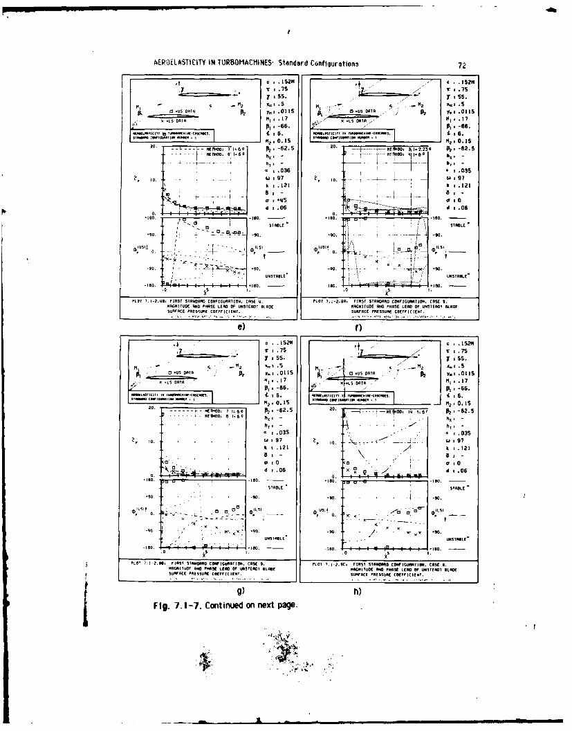
AER13ELASTICITY IN TURBOMACHINES. Standard Confiourations 72

Se. ..152M ,- .1527 T .7s .55

7 55. - :55.

1 -y: .0115 p , A -US DTA .0115

0X1 .17 .4: .17p1 -66. Iv -66.

: . wwALRI .:. E V... ....... ... . [ : 6.M2: 0.15

M, 0.IS

A. H"00, 7 16o0 -62.5 R0.E 31=2.230 . .- 62.5RE OD, A 1=60 ht OO. A g. 6 A.... .. L' '""0 3 1

Xm

.036 :.03S10. wa 97 t, l . .. . 9

k .121 k .121

R4- X,a -4 +,6 ----- ..... . J od~ .06 d .06

. "0A . . .. .4[-100 - O

, J eLSTABLE .. STABLE

0 - 0 .- -0. o90. i

-90. . p "0. r- - 9 0.

USIA--555 -U 0.

-9.0 e O.: _.. .oo TAL E

-lA. "mi I I flT.-10 AL~t~ ~j - I so.0

-9k. . ' x .o -s .0 .50;- x .o

PLOT TI-P.AB: FIRST STANDARD CONFIGURATION. CASE A. PLOT 7.1-.9 , FIRST STANDARD CONFIGURATION. CASE 9.MAGNITUDE RNO PHASE LEAD OF UNSTEADY ALADE RAGAITUDE AND PHASE LEAD OF UNSTEADT ALADESURFACE PRESSURE COEFFICIENT. SURFACE PRESSURE COEFFICIENT.

e) )

c .152M4 C I * 12T .75 r:.75

a - - 7:~~~55. ~~'' 1:5.

MI .5 2, AIR M2 Sp 0 -US DATA .0115 p3 USATa

X .LS DATA m . .17 4.f . L XATF-M 1.17] _ p:-66. k .1,-66.

MU!~~~ -"IIAS IB LS:T~ fS tRs0 . 1 6.:.ITm, UO IG R... I, IJ 0 IS

20. . - ETO, 1=60 i2 -62.5 20 . H RET1ROD, '6 1=61 p2,-62.5R.E 0 . 60 A-: - , .1 0h, -

T' - -,. . - " -0T'

.035 0 - 3

?, .w 197?101 u97k .121 k " 0 .121

a 8 -

a 1 0 a 1 0Is 1 .06 . d . .06

"*'0 STABLE f STABLE"90. ' '• -g0. "90. -90.

0s'! oS e. • " 0 1151 ___ o - C. 0 LSI

* U - .. a.... lU- t: - -x

a90, "90. -90 / '.

/ a-'"0 UNSTABLE . UNSTABLE'

-1I0. I9 4 6 0 10 IRE. 1 -0 .0

PLOT TI-PA, FIRST STINRA O CONFIGUONATION. CASE A. PLOT T.I-.it FIRST STARANR COW IGU TION. CASE A.NGGITUOF AMI PHTASE LEA" O UNSTEADT BLADE NAG"ITUOt AND RAI LEAD OF UNASTEADT BLADESURFACE PRESSURE CUFFICI EAT, SUAFACE PRESSURE COEFFICIENT.

g) h)

Fig. 7.1-7. Continued on next page

A

".75

... 7 S 55. .. ": 55.

,- M Xj. t.. .5

4 pX .'5 .0115 X -LSo?M2_ .16__ _ _1 pT M? . .0 5

n ac~ . ---a - ...i- ,,scf c oos I.-: TO I * -2 o. ----.-------,-- 7.,c h ic .rTo, , -(. 1., -2.

20. ...... T . " I3 1-0.27 -62.. . 0, 3 ,,,, -0. EMEHD 4g 1.202 kx o

*.009 !.009w sJ 9797

• *0 . . .. -, .1 * *. 0, -1+- - , . 12x -ys, -yd 0 Al t.06

0.[

0. USS4 ILO""go"5 ---. .. -2 o -*9 "' ... X....t".....".....L ,.

UNSTABLE. UNSTABLE"

,o80 M. -1..o ,

PLOT FIRST STANOAO CONFIGURATION, CASE I. PLOT 1.l-2.?0tFIRST STANDARD CONFI GUMTIO. CASE 2.MAGNITUO ANID PHASE3 LEAD OF TUUNTERO BLADE

SURFACE PR005UR1 COEPPICIOII0. UAT CE P ESSURE COEFFICIENT.

1) ,1 )

c.,1521r : .75, ,55.

._/ . Fig. 7.1-7. Unsteady blade surface

-, D -62. pressure difference coefficient

toU.Mi*** Ki 1*.. mow-T*. : 2.e *1001 W I I M, 0. 06 versus chord for different

R - P0.7 -62., - interbiade phase angles

S * .009

0 n97IT 1 .22

4"" -" ', I- IF '1 ." -, 8 --

PLOT ~ ij k,~4? 101.06

". 1 F.J E1l-. j- , t

0.

1.I20, SK0 0110COP0.510-180. .180i.

01 11 00 1.10 0 * 10 0 O L~PLTTI2 tFIRST STMOAN I ORIG~mT am, C0151 2,

wmWIT UK AN P"ASEi LEADO OF U S rEgrT KnRe

SURFOCE PRESSURE MY ICIIIIT.

K)

I

AEROELA3TICITY IN TURDOrIACMINEM: 3tanOard configurations 74

However, the same argument cannot be used to explain the differences inphase angle in Fig. 7.1-6b (which in any case is much smaller than the ones inFig. 7.1-6d), as in this case the values of the real parts of the pressures on

the lower and upper surfaces are further apart. (The difference in theimaginary part betweeen the lower and upper surfaces of the blade is of thesame order of magnitude as the difference in the real part.)

In this context, the interesting investigation of different vibration amplitudes

performed by Carta in 115] can also be discussed. In Fig. 7.1-5 (copied fromref. [401), the experimentally determined aerodynamic damping coefficient is

represented for 0.50 and 20 vibration amplitudes. A slight difference is foundat a -450 interblade phase angle which, by investigating the surface pressures(Fig. 7.1-Ba,b), can be attributed mainly to differences in the first 10% of theblade. Again some slight disagreement, this time between the two

experiments, is found in the lower surface phase angles in the second half ofthe blade, where the amplitudes are small. However, the trend for bothvibration amplitudes is identical.For other cases, presented in [15], the pressure amplitudes in the leading edgeregion show smaller differences between 0.50 and 20 vibration amplitude than

in Fig. 7.1-8. This is confirmed also in Fig. 7.1-5, as the experimentalaerodynamic damping coefficient has almost the same value for both vibrationamplitudes. But also for these interblade phase angles, differences appear inthe phase angle of the lower surface pressure in the second half of the blade

(see Appendix AS). A detailed investigation of the data in [15] indicates thatthese differences are probably due to run-to-run variations in the unsteadydata, and not to nonlinear effects. This can be concluded from Fig. 7.1-9 and7.1-10, where the values

l*p =# p ==-# p o=0.5

are shown for two incidence angles, i=2 ° and 60, at 77% and 6% chordwiseposition respectively, for both the upper and lower surfaces, as a function ofthe interblade phase angle.In these diagrams, it is seen that:

* The scatter in Op is larger on the lower thai on the upper surface ofthe blade in the 77% chordwise position (Fig. 7.1-9a. b). A possible

explanation for this is that the pressure amplitudes are smaller on the lowerthan on the upper surface of the blade. The accompaning smaller signal/noiseratio may influence the accuracy of the phase angles.

4 .. •"~,

tPr-Lausanne, LADORATOIRE DE TIIRMI QUC APPLIQUE T DE TURDOMACHINC3 75

* The differences in 641 are much smaller in the leading edge region(x=0.06, Fig. 7.1-10a,b) than in the trailing edge region (x=0.77, Fig. 7.1-9a,b). Again this can be explained by difficulties in determining accuratelythe phase angle by small pressure fluctuations.* The scatter in 60ip, both at the 6 and 77% chordwise position, is

approximately the same for both incidence angles (i=2 ° and 60), whichindicates that the unsteady flow and the experimental accuracy are similar inboth cases (Fig. 7.1-ga,b and 7.1-10a,b).* The scatter in the absolute value of 6Ep is approximately the same for

the lower and upper surfaces and for both incidence angles in the 77%chordwise position although, as mentioned earlier, the pressure amplitudesare in general smaller on the lower surface (Fig.7.1-c,d).

.1521 c .151

7 :55. 7:55.

M i . M 2 . 5 "" 2 x =7 . 5p 09US DATA Ya: .0115 p3 -' IUDAya .0115Mi, .17 , .1DA-LS DATA 1 .7'. C-I DATA M, .17P , -66. -66.

-L-111CNI MI fl1 C S MW 1 6. 1.SIT 2StS:$ 6.Ha ,___ - :0.15 3'2 0.15

20. P ................... I = 2.262.5

h - E D, hTm -

a .009 I a .035', ,o. 1 97 , ,o. * u :97

k .122 t B :.122

o . ." ' " ... x -- i

,"STABLE j STABLE

-90.D. 90. --"0;..- . .

'XIAI X ISX ....

x l x r x iX z x x x -,I, ®L, w, I;A~~~pr0 D. -__ 01 __ IU

-90. .- - AD. -90. -g- - -50.1,9 -UNSTABLE"L

-IO s . ... 0.. . . " T0 L -T0. S. .

S k.

PLOT 7.1-2.3, FAST STAAD I O CONFIGURATION. CASE 3. PLOT 7. -2 ,5. FIRST STAOAD CONFIGURATION. CASE S.AG E UTDE AND PHASE LEAD OF UNSTEADY BLADE RANITUDE AN PASE LEAD OF UNSTEADT BLADESUAFACE PSESSURE CEFFICIE .T.

Fig. 7.1-8. Experimentally determined unsteady blade surface pressuredistributions for two vibration amplitudes (a = 0.009 and0.035 rad.)

-t - ... II I I

AEPOELA7[.-T ,~' IN TUR*Cf1;I-!!NEC

-180 0 180 -180 0 180

601 -* A A

120- 120- A- 120

A

o 0 A A A

*10 001- A A

0 A i=60soo-12 -1 0 A A -o 2

-180 a 18-00

a) upper surface b) lower surface

I I I I

20- 6 0 .0- ,0- .0

0 A0 e 0 0- A A A 00 o co AAA A ,

0 00 00 00 AA A A At

-2.0 = 20o -20- A ,& -2.0

A

i2

-180 0 a 180 -180 0 a [so

c) upper surface d) lower surface

I I

2.0- 0 2.0- 6p'Ela- 2,0

0 A 0 0- 0Aj A A

6

-2,0- -2.0 -20

o us us:I I

-l1O 0 a I8 -180 0 a I0

e) :2' f i=60

Fig 7 1-9 Pressure coefficient and phase angle differences between 2"

and 0 5" vibration amplitude on the lower and uper bladesurfaces at 77 4 chordwise location (i = 2*, 6' k = 0 12)

EPF-Lmasne, LAOORATOIRE DE TtlCRflgUt APPLWOUrE CT DE TURBOMACtiINE3 77

120-ba 120 6*ap120

-120- oi=2 -120 A= 12: --120* i=60 A i =6

-18o a * IS0 -180 a 1806) UW1e Surface b )lower surface

2 AA

o* 6 A A 2

0-0 0 A A A 00 9 A A

-2 -00 -2 AA-2A A A

-4 i=2 A-4 A --4

-18 ISO16 -180 a180c )upper Sur face d) lower surface

2 - */4a z 2

0 31b &ao 0 46 0

-2 Ut] us1u-2

g, 1=2 f) i=:5

Fig. 7.1-10. Pressure coefficient and phase angle differences between 2*and 05S' vibration amplitude on the lower and upper bladesuraces at 6 X chodwise location (I = 2*, 6' ; k = 0. 12).

ACROELAOTICITY IN TURDOt7ACMINE3. 3tanaara conriquretions a

* In absolute values, the scatter in , s larger for the 6% than the 77%

chordwise position (Fig. 7.1-9c.d and 7 I-lOcod) However, in relative values

(6Ep/Ep0 =20) there is much less scatter close to the leading edge, as here the

pressure amplitudes are higher (Fig. 7.l-9e, 7 I-10e)

* The differences in 64 seem to be independent of the steady incidence

angle.

From Figures 7.1-9 and 7.1-10 it can thus be concluded that a possible

explanation for the disagreement between the predicted and experimental

phase angles in the after part of the lower surface of the blade is run-to-run

variations in the data.

[P-.Leusnne LABOeATOIug Dt TnlrItnOU APLIftM Ey of WuRL M&CIP K

Cesliusliss for tMe First Stamierd Ceft glurutie

From the controlled excitation work in traveling wavt mod* 0e constant

interblade phase angle between all blades) on a 6X thick conpres$or cLascade

with 100 camber in the low subsonic flow region, it ran be concluded that

* It is todaJ possible to predict Kcurately the aeroelstic behavior of a

thin, low cambered compressor cascade oscillating in traveling wae mod in

low subsonic two-dimensional flow* The good agreement between the unsteady exenmental data and

predicted results mutually validates both approaches Where disagreements

are found, it is not possible a priori to exclude either theoretical or

experimental inaccuraCies* For this specific cascade, the predicted time-avaged results agree

better with the data if the theoretical incidence is slightly modified (Fig

7 1-2) However, the agreement betwee the time-depe t predictions and

data is better if the experimentally determined incidence angle is used for

the analyses No explanation for this apparent contradiction has yet be

found (Fig.7 1-5)

Conclusions for eroidynalc daing.

0 The theoretical models accurately predict the stability limits for the

cascade, using the assumption of zero mechanical damping (Fig 7 1-3) The

shape of both the theoretical and experimental damping curves is identical.

but the magnitude shows disagreement This would be dangerous if a non-zero

mechanical damping is assumed in a design phase, as the different prediction

models would then give different stability limits

0 The stability limits of the cascade (with zero mechanical damping

assumed) is predicted Just as well with flat plate theories as with other

models (Fig. 7 1-3) Discrepancies are however present in the magnitude of

the aerodynamic damping coefficient. For conservative stability analyses

(zero mechanical damping), flat plate theories thus seems to be sufficient for

cascades of the kird used here.

* Neglecting the blade geometry (i e. using a flat plate model) apparently

has an effect of the same order of magnitude on the aerodynamic damping as

that of neglecting the incidence angle (using 0° incidence)

~ rf.~c p~s~-e diffrerict coefficient

* ~ ~ 1) ' . 'he*I.t rntI.? - nd thp )no,, vith the true qtometrU agreett. ~ ~ ~ ~ ~ 1 'ry ej'' i~~ ~ r, the unsteady blade surface

0 Thip *.r( Imi~~ 1-n i, urri~i Dredcied witfi all methods The

-I'igifuij- -lqlii 0jiqPVllefj with some of them 'especially the flatL116 , 'rtule'.[ I

* In most rase-, file Dhase anqlep 060 of the unsteadyj blade suirfacepript,,ure dlifferonce toeftfeitit Dririted well Some d1sagreementS Can

pOffbI'N oe euiplairied bu run-lo-run variations in the data amd by~ the data,oloui lion pia'H al~uro for fair ulat inq A and g

* Tho small disagreements in aerodynamlic damping between theories and.yporiment (Fiq 7 1 3 1), can sometimes be traced to dissimilarities in the,implitude of thep blade surfacp pressure difference coefficients, andsomelimobs to Ihe ph'ase angles l~ig 7 1-6). both for the experiments and theanatrjse,

* A large part of the aerodynfamit damping comes from the leading edgeregiont For an accurate experimental evaluation of this parameter it isimportant to measurep the linsteadli response cloise to the leading edge (whichwas doine in the experimnental wonl serving as base for this standardconf iguratitorn 1151)

Lonclusions for the unisteady blade surface gressures

0 The local unsteady blade surface pressure coefficient on the upper andlower surfaces is also predicted well The amplitude shows a particularlygood aqreemera, Mween the experiment and the separate analyses* The local phase angle (#, (US). * 03)) trend is captured well In some

cases the magnitude, especially for small pressure amplitudes (i e lowsignal/noise ratio which might indicate data inaccuracies), shows some slight.disagreement between the experiment and the analyses (Fig 7 1-7)* The largest disagreement between the experiment and the separate

analyses is found at a 00 interblade phase angle (Fig 7 l-7f,g,h) rhisbehavior can perhaps be explained by the small pressure amplitudes in theexperiments for this Interblade phase angle. The analytically determinedacoustic resonances are also close to a 00 interblade phase angle, whichmight influence the theoretical results.

I •

Pt-L&ueuube, LADORATOIRE DC TMCRrIQUE APPLIOUM[ rT VE TURDOMACIMN[ 01

7.2 Second Standard Configuration

Definition

This Incompressible two-dimensional cascade configuration has been mea-sured in a water cascade tunnel at the University of Tokyo. The results havebeen submitted by kind permission of H. Tanaka 119-201.The cascade consists of eleven vibrating and six stationary double circulararc profiles. Each of the blades has a chord of c=0.050 m and a span of 0.100m, with a camber angle of 160 and a gap-to-chord ratio of 1.00. The watervelocity during the tests was v1=2.4 m/s, with the Reynolds number at

Re=1.2* I05 .The eleven vibrating blades oscillate In pitch, with an amplitudeof 0.059 red (3.40) and a frequency between 1.3 and 13Hz. Thus, the reducedfrequency lies in the range 0.1 tol.O.The cascade geometry is given In Figure 7.2-1 and the profile coordinates in

Table 7.2-1.Experiments have been performed with Incidence ranging from attached topartly-separated and fully-separated flow. Further, the stagger angle as wellas the interblade phase angle and pivot axis have been varied systematically.The experimental data indicate the unsteady lift and moment coefficients(amplitudes together with the corresponding phase lead angles). Thesecoefficients are computed from strain gauge measurements and no time-dependent or time-averaged pressures are measured on the blade surfaces.

Aeroelastic Test Cases

From the large amount of data obtained during the experiments, and from the

sample presented in (4, 201 0 aeroelastlc test cases have been proposed(Table 7.2-2).All 0 correspond to the same steady-state configuration (stagger angle = 300,inlet flow angle Pl=-300, M1 =0.), and the interblade phase angle is varied.

ACROCLAZITICITY IN TURflOMACttINE31 316ndard ConrgratIOA3 02

Low SsQma m(npm a Proile.

cascade leading __________

edge plane-

upper surface

Vibrati ~ ~ ~ ~ ~ ucin surtfaced(x,~)(.50032

d = (thickness/chord) = 0.05240( = 3.40 (=0.06 rad)c = 0.050 m P1 = -3001' = 1.00 camber = 16.80'k = 0.4 1 =30spa= 0.100 m a = variableWorking fluid: Air

Fig. 7.2-1. Second standard configuration: Cascade geometry

WP-1.411113AR4, LABORATOIRE PC TIItll APPLIMUC CT DE TURflOrACIlNE3 85

Double Circular Arc Blade

c=0.050 m (1.968 in.)

Suction surface P-osaure surface(upper surface) (lower surface,

M () y ~')y

0 0 a

5 1.644 -0.404

10 2.637 -0.127

15 3.509 0.115

20 4.262 0.326

25 4.897 0.505

30 5.416 0.650

35 5.818 0.764

40 6.105 0.845

45 6.272 0.893

50 6.334 0.910

55 6.272 0.893

60 6.105 0.845

65 5.818 0.764

70 5.416 0.650

75 4.897 0.505

80 4.262 0.326

85 3.509 0.115

90 2.637 -0.127

95 1.644 -0.404

100 1 0 0

L.E. and T.E. RADIUS RADIUS CENTER COORDINATES

L.E. RADIUS/c =0.666 (%) x=0.666 (A), y =0 %T.E. RADIUS/c =0.666 (%) k 0.993 '%), Y= 0 %

Table 7.2- 1. Second standard conrlprton: Dimenislonlms airfotIcoordinates.

A(RI-(L A5T1Tr $TY IN TUFIOtIACIIIN[:. 5d4Ai6id kCunht~q etIOri 64

.- j '. L . T ., I fp. - I t Wn

For the moment onti4 one mnethod (Method 1) has been applied to this standardcnnfiguratlon The reason is the resemblance to the first standardconfiguration, in which the time-averaged and time-dependent pressures werealso measured on the bladesN4o detailed comparison between the experimental data and the thereticalresults can therefore be made presently However, Fig 7 2-2 gives anindication of the expected resultsHere, the predicted blade surface pressure difference coefficient (AEP) ispresented for two phase angles (o=- 1350, 00. Fif 7 2-2a~b) together with theaerodynamic moment (em) and damping coefficient (3) versus the Interbiadephase angle (Fig 7 2-2c.d)it is concluded (Fig 7 2-2c~d) that the same trend exists for the experimrientaldata and the results predicted with the flat plate analyses (Method 1)

Atroelastic Time-Averaged Pa amters Time-Dependent. ParametersTest Case vi 1 0i 1c kNO (mis) (0) (0) (HZ) H- (red) (

12.4 30.0 - 30 6.1 0.4 0.059 - 1352 - 903 - 454 --- 05 * - 45

6 + - 90

7 + - 1358 - - -- - 160

Table 7.2-2 Second standard con? "gwtion.8 recommended aerolastic test cases

9fO-L"SOOM, LA6OVATOh t3 TIRWOU AP91.tOtIM t V Ot TUOMAC"IMN! 0

iowever, judging from the theory. some scatter seems to be present ir, the

expernmentally determ led phase angle #m. which can most clearly be seen inthe veroatnemtc damplnq coefficient (Fig. 7 2-2d) The trend for theamplitude of the moment coefficient shows a better agreement (Fig 7.2-2c)although the flat plate theor predicts slightly higher values than themeasured ones This agre s with the results from the first standardconfiguration (comrre Fig 7 1-3b and Fig 7 2-2)

86

T .0 .1.00

30. 30.

96: .0"62 Y. 1. .03620

1 -U a:s W

0,. -3 P, -30

PNO -aemic IP.

u36. 4 w . u3.45 0.4 k 0.14

-13 ora1OS.024 d 0524

0,

0~~~~0 A ~-. 0,~__

C 0. .1 0 OM

r~30 30.~ o c~re I IIStS ?6 tWIUO S.(3

01 06, V36 0.03 PITW U 1(0 0.I 036~KP!i.~0 ~AoI 43

If 0. -. .o -0.5

AN, 1.0?..0

, 0. . 0.S

k t* 0.5 1 0.4

IS P. 0. If. 30.0

40 11-0.0 17 4 .- 1 N

A-6 00 0 My IICIIIC0,~l ED ERO wt ef e A IW.CarICIt 1

Fg 7.-. Seon 0.adar -on Sira 0.14d srac resr

difeene moetad apnoefcet

4-002 00

EPF-Lausenne. LABORATOIPE DE THEPMIOUE APPLIOUEE ET DE TURBOMACHINES 87

7.3 Third Standard ConfiguratIon

Definition

This quasi three-dimensional transonic turbine configuration is being tested.in freon, in the annular test facility at the Tokyo National AerospaceLaboratory The experiments are included here by kind permission of H

Kobayashi.This configuration, standard configuration N*3, is used with outlet conditionsranging from subsonic to supersonic flow velocities.The cascade configuration consists of 16 vibrating cambered (60.8)prismatic turbine blades. Each profile has a chord of c=0.072 m, with a spanof 0 025 m and a maximum thickness-to-chord ratio of 0. 124 The staggerangle for the results presented here is 45.70 and the pitch-to-chord ratio is

0.763 (hub)0.804 (mid-span)

0 873 (tip)The hub-tip ratio in the test facility is 0.844The profiles are oscillated in pitching mode, around the pivot axis at

(0 195, -0 1097)The cascade geometry is given in Figure 7.3-1 and the profile coordinates in

Table 7.3-1The working fluid is freon gas, with the specific heat ratio = 1 137 (Freon-II, CFCl 3 ).

Experiments are performed with a variable expansion ratio (Pz/PlV, M2),

oscillation frequency and Interblade phase angle. All experiments are

performed with constant spanwise upstream flow angle and flow velocity.The time-dependent Instrumentation Includes pressure tappings on a blade(midspan) and strain gauges The unsteady moment coefficient is determinedwith torsional cross spring bars,

AEPCELASTIf ITY iN T E.r: Nr tf L 'onfgur i88

d = (thickneeschred)surface

cx ~ ~ suto sufc 0.l2aM2I~nl kvral

0.873sucio (tp)hr/tpace84

var=ab.0 a72 675 (nominal) vral

Work ing fluid: Freon- I I (CFCI 3) With specific heat ratio = 1. 137

Fig. 7.3-I1. Third standard configuration: Cascade geometry

ILI

EPF-Leusfine, LABOROTOIRE DE THEPMOU&JE APPLIQ'EE ET DE TUROMACHINES

C -0.072,,

(Lw surface) (Upper surface)x y

0.0 0.0 0.0 0.0

-0.073 -0.0090 0.0247 .0.0108

-0.0115 -0.0Z90 0.0439 00.00"

-0.0OS. -0.0487 0.0711 -0.0073

0.0102 .0.009W 0.0932 -0.0144

0.0296 .0.0918 0.1213 .0.026S

0.0462 -0.100 0.1478 -0.0356

0.0068 -0.1240 0.1742 -0.)434

0.0887 -. 1384 0.2014 -0.0$02

0.1117 -0.1508 0.2289 -O.0S38

0.1358 -0.1610 0.2563 -0.0601

0.1606 -0.1093 0.2840 -0. )637

0.1804 -0.1749 0.3119 -0.0660

0. 21 Z2 -0.171 0.339S -4.074

0.2354 -0.1797 0.3676 -0.0676

0.584 -0.1800 0.3891 -0.0069

0.2814 -0.1793 0.4113 -0.00 2

0.3046 -0.112 0.4329 -o.06S7

0.3274 -0.174S 0.4547 -0.0046

0.3432 -0.1719 0,4765 -0.0639

0.3591 -0.1692 0.4982 -0.0623

0.3748 -0.16S7 o.s201 -0.0613

0.3904 -0.1621 0.5419 -0.059,

O.40SS -o.150 o.S035 -o.os79

0.48" -0.130 o.58so -0.056 ,

o.s552 -0.1208 0.6069 .0-0540

0.6291 -0.1018 0.628S .o.OS19

0.7038 -0.0829 0.6soz .0.049,

0.'780 -0.06040 0.71 .0.0470

o.8szs .0.04sz 0.939 .0.04,6

0.9270 -0.020 0.7152 .0.0419

1.0 -0.0075 0.73" .0.030.7583 .a359

o.726 -0.g2s

u.9387 -0.037

0.8792 -0.01760. AgS -0.0118

0.9597 *0.00W

1.0 0.0

Tale 7.3-1. Third 3tandad configurlaton: Dimensionless airfoilcoordin tes (spmwIs Identical).

Pli. in~iedi presiurpi; ar-; TwasurpO -01h .1 hiqr-res~onso jeS

IranSducer located outside the test-rig, and a calibration for losse-,;i Irequoncki and amplitude in the pneumatlc tubes4 S DerormeO

Aeroelastic Test Lasts

iri the resulltc obtained from these expenmont 9 aeroelastiL 'Ps' case,risve beN proposed by H4 Kobayashi for off-design calculation !46! Thesewere defined after the Cambridge Symposiun a&d thereforp do not correspondwith those presented in j41 The data wort also received late in the projectand for the present no attemvpt has been made to calculate the aeroelastic

behavior of this standard configuration Therefore only the excperimental dataare included here withoout theoretical results It has thus not been possibleto validate either the time-averaged, or the time-dependent data10

The aeroelastic test cases proposed by~ H Kobaashii are given in Table 7 3The corresponding time-averaged and time-dependent data are presented in

Fiqs 7 3-d2 and 7 3-3 respectively, and in Fig 7 3-4 the measuredaerodynamic damping coefficient is given in dependence of thie reducedfrequeincy

9 Details about the cascade, instrumentation and data reduction waspresented by H. Kobogashi at the 1984 Cambridge Symposium on Aeroelasticity145).10 The comparison with theoretical results will be especially interesting asthe idea to use pneumatic tubes for the unsteady pressure responsessignficantly reduces the experimental costs (see 1451 for details).

EPF-L&Usenne. LABORATOIPE DE THERMIGUE APPLIOUEE ET DE TUPOOMACHiNES 91

0Z Time - Averaged Parameters

-LI

0

0 M, PI PW21PWI PIIP2 P2

I - 3 0303 - 1.2 0964 0.778 0662 - 58.3

4- 6 0334 - 1.1 0.946 0.432 1.242 -56.1

7- 9 0319 -1.2 0.664 0.345 1.390 -55.5

Time-Devenaent Parametersmt i =Interolae ponase an 1e measured

Amplitude (Nominal 0 Cti745-rad) $ aseto . - ~, __C tomn al .50)..(-2) T 1 2) : C5 o

F (~(a)Hz)f Ku(0 (0) (0) (0) 0

1 0.965 0.952 0.0172 0.996 1.028 25 0057 65.5 73.6 66.6 679 70.2

2 1.006 0.973 0.0172 1.026 1.032 1000.229 76.4 67.4 67.6 646 705

3 1.087 1.024 0.0171 0.966 1.075 2000.457 71.2 68.7 71.8 68.5 707

4 0.965 0.952 0.0172 0.996 1.028 25 0.031 65.5 73.6 666 679 70 2

5 1.008 0.973 0.0172 1.026 1.032 1000.126 76.4 67.4 676 646 70

6 1.087 1.024 0.0171 0.966 1.075 200 0.251 71.2 687 71 C 685 7-r

7 0.965 0.952 0.0172 0.996 1.028 25 0.028 655 736 666 67- r4

8 1.008 0.973 0.0172 1.026 1.032 1000 112 764 67 4 67 E, 6,

9 107 1.024 00171 0.966 1.075 200 0223 712 66 7 7 1 6 6H

Table 7.3-2. Third standard configuration: 9 recommenoed aeroelastictest cases (Fluid used is Freon- 11; all values are at m idspn)

'AD-AISI 763 ELIAI 0 S 2/3

UNLSIIED AQLCElAL.. 198 AFO S-IB-O F/G 13/7 ML

L AN~

1 25 Ui6

I ____ ______

AEP(IELATiC.IrY IN TUiP5Ur'ALiNES Standiar'j Cor,fi iur .oh,-I 92

I C .. 0721 e.072

P1 . 4 ~ 5.70 i .... 7 sUS.70M, X 1 195 P~ 12 z .19S

P 2 p,,:-II.110P

a _ _ __ _ -US -A526.100-U n lPT 5.3 "1 .33

PI~ -1. P, -1

A 142 0.8M, .4

IT, , -S. P2 - -- S-----t

III I . 121

I'~0 S H-,

x x

P T.3I THIRD SANDRD CONFIGURATION .CASES 1-3, PLOT1 7.3-1.2, THIRD STANDARD CONFIGURA TIRW A SE 4 ae I-A,TIRE AVERAGED OLAIDE SURFACE PRESSURE ITIME AVERAGED IIAI SURFACE PRESSURECOE FFICIENT. CCOEFFICIENT.

a) b)C .q72

M, T:.8041

4S11.70

A~m-S OA P2 Y.,:-.110M, .319

P, -1.2

WlT ' MUNI . M2: 1.390

d 1 12.4

0. TITx

PLOT ~ ~ 7.-..TIDSADR CNIUAIN CSS7TIM AVRAE -LPESRAEPESR

COEFFICIENT

C I

Fi.7.-. hrdsanad ofiuaio.Tieavrge laes-fc

pressure ditiuinfr- .8 .4ad13 eP

I'd .11

Lt'r-LU3afilcLAD LIUK, UI, t utI tiEfPIOU APPLIUUEE ET VE TIJR6UIMACmINES 93

c .072Iq c .072M

. 00q FIT .804

2 Ia. -. .195

S. 1 10 " I -I10."03 . . . .303

-a .682 ON , P, .682

P.-56.3 P2 -58.3

s.0172 a.0172

1S7 t, 0. -,3a628

S x 1 .057 k .229

.r a 67.5 - a t67.5d s.124 Xd t .124

i UMTAO[NM i UInRLE

SIOSE551

- o. ' '. . .o.- -5. . . a - - a 0.

PLOT 7.3-2. 1, THIRDO STANDARRD CONIFIGURATION ,CASE[ I* PLO 7.-2alTH STANDRD CONFIGUfRATION , S 2.1[a

MAGNITUDE AND PHASE LEAD Of" UNSTEADYT SLADE H:GN|TUDE AND PHASE[ LEA0 O NTEROT BLADE

SURFACE[ PRESSURE CO[IICI -#T SURFA EI PRE[ LINE C E[FFIC ENT.

a) b)

-0s. 7 1 /2 .

... Alaas M25 X.z : . 195- as Y. -.0 , I s -.110

, .303 M , M' , .334

-0. P0. hA, -. 1. 072

.01 72

It .3t MkI .031

x x !jx a67.5 Px67. 5

<x I .12% x d .12q-ISO. , , 5 . - 0. -to 5.-90. 90. -- IS

_ LSI Ba-110. xT X,

.. .0. -- _e' -I ID. -S0. SO -ISO.

UBSTASLE[ ,a UNITASLE"

-,o0 .0 . . .. a,0o _ .,

PLOT 7.3-2,1 THIRD STOIOiA CONFIGUATNIO N CASE 3. PLOT 7.3-2.0, THIND STiAIOAM CAFIGuaO m - CAiSE 4.WHITMS . m P.tNSE LIAO OF U LSTEADY SLAOE ARGNITUOE ANE PHASE LEAD OF UNSTEROT SLADESRFACE PRE0SUME C09PFICINT. SURFACE PRESSURE COEFFICIENT.

c) d)

Fig. 7.3-3. Continued on next pagedW-

0 _ .

AEPOELA TiCITY 'N TuP6OGMACHINES: 5tandard Configurations 94

0 072H.072 M1

9 ~~m .80804~

745.7 4S 711.74 t.195 -M, .195

i,.334 M, .334

,1Uatic'. E:,AM: 1.242 Mo,.. 1,3- H2 140. -56.1 0. P2 -56.1

* B.0: - -- -- - -- El - -iB, -

= .0172 i ! : .0172

- u628 ~ ,O.*----i----S--iw12S720., f r, It~ t1 k.t26 1 A :.251

mxx d:.1 4 x d . 12

6 =. , - - __ 86. o:7.D . -+-- 0. t -.~ 1

tSTABLE STABLE00. I -IO0. -90. - , -, - , -980.9 -- W [ -1t .9o

Cr'sl . OIS) 4lU~ x 0S0 -~-x"-,- I p 0. ,T ,x.-, ,-

-90. ---- .9o -90.UNSTABLE' UNSTABLE=

0 1. 0 1. 10L0T 7.3-0.5:St l STAI NDUADO CONFIOeURBilON ,CASE S. PLOT 7.3-2.iii THIRD STANDARD CDNFIGURATION . CASE A.

HAGNITUDE AND PHASE LEAD OF UNSTEADY BLADE AAGAITU8O AND PAASE LEAD AF UNsIrEAO BLADESURFACE PAESSURE COEFFICIENT. SURFACE PRESSURE COEFFICIENT.

e) f)

• r : .804 . 07

* / 7:745.?7 1 74.5.'US DH H , ,:: A TiPRoc, .

le 1 . 95M 2 45:. 79P2. ," -. 2x,,105 I" .85 IATA P2 _- k I.1

., IS: l .319 M, .319P,. -. 2AP :-1.2

M2. 1.390 M2 1.390

-- 4 - g-

8,- - d x x

X67.5

0. -4 . . . .- ,-4

-90. p I Olt STABLE STABLEt -9. -9, - 20-

U 0. x1

X! , II

90. 90. 090.

UNSTAB UNSTABLE'

.0 .0

PLOT 7.3-2.7s THIRD STANRDAHA CONFIGURATION , CASE 7. PLOT T. HR-2.8, THIS STANORAiD CONFIURIION . CASE B.OROITUDE AND PHASE LEAD OF UNSTEADY BLADE MAGNITUDE AND PHASE LEAD OF UNSTEADY OLA0ESURFACE PIESSURE COEFFICIENT. SURFACE PRESSURE COE FFICENY.

h)

Fig. 7.3-3. Continued on next page.

EPF-Lausenne. LABORATOIRE DE THERMIQUE APPLIUEE ET DE TURBOMACHINES

.072H

:115S. 7

- .195_D uspa.,-.,,0P1 , -1.2

M,, 1.39710. -. P, -55.5

0 [ h, -

0 9 .0172el :12S7

k t .223

-at

" 67.S

-190.

-90. 90 S TABL

0, 00.sI 0 4 0lLSII

* o. -

-20 .90.

U StOSeLE"

PLOT 7.3-2.9, TWAO STf5ORO CONFIGURATION . CASE S.AONEITUOE ANO P"06 L.R0 OF UNSTEROY OLAOSURFAICE PAESSURE COFFICIENT.

I)

Fig. 7.3-3. Third standard configuration. Time-dependent blade surfacepressure distribution for the nine aeroelastic test cases

12t ,'rL A-li, II . Y 1N 10. b 1: I1_ L M 1/' tartojard C ontigur"ati . .

MI. .072K , .072, )' ,.8' Ph".804 II I- .ON

7 45.7 Ills , .7

f,.195 Its

C3 S 2 OATMI .303 MI .334

6H z ,~ ~ *~AR 4 0.682 ' OA' M, 1.242-4.PFIT5 PIT

S.--

MI. - by, w -

-2. . ~ a8 -...

o:67. S a 1 ' . ,,67.s

* d .1 2 II I* .. 12 I0. C .USTP F I

• 2. 1* *

0. 0.25 0.50 0. 0.10 0.50S

PLOT 7.3-6.1, T.IRD 5TANDARD CONFIGURATIOS. PLOT 7.3-6.2 HI0 StANAR COWPG|RPTION.

A RODYNAMIC WORK AND0SHPIO COFFICIENTS AERCOTNMIC MORK AND DAMPING COEFFICIENTS

IN 0(PENDENCE OF RCOUCC0 FREQUENCT. IN lEOptSoSu" OF SRtMl O FSUIE"Cl.

a) b)PI c7 , .072"

7 1"5.7

M2 _. i' 95 Fig. 7.3-4. Third standard configuration.

,. .303 Aerodynamic damping coefficient

- -.A5TA -P, 1.397 versus reduced frequency for

M2 0.68, 1.24and 1.40 resp.hT -

d ,67.5'# d .121 /

. - . , -NT- qTB

°2.

0. 0..5 0.50

STBS

PLOT 7.3-6.31 THIRD STANO O CO 0UMPTION.AEROOtNAMIC OIN AND DAMPING COEFFICIENTS

IN OEPENDENCE OF REOUCEO FREOUENCY.

c)

" " "C T-.. ...

EPF-Lausanne, LABORATOIRE DE THEP.MIQUE APPLIIEE ET DE TURBOMACHINES 97

7.4 Fourth Standard Configuration (Cambered Turbine Cascade In

Transonic Flow)

Definition

Ouasi three-dimensional cascade experiments on high load turbine rotor

sections are being performed in the annular cascade facility at the Lausanne

Institute of Technology 122). The experimental data have been made available

by Brown Boveri & Co and are included in the present report by kind

permission of A. o61cs [21-251.

The fourth standard configuration is of interest mainly because it represents

a typical section of modern free standing turbine blades. This type of airfoilhas relatively high blade thickness and camber and operates under high

subsonic flow conditions. It normally exhibits flutter instabilities in the

first bending mode.

The cascade configuration consists of 20 vibrating prismatic blades, each

with a chord of c=0.0744 m and a span of 0.040 m, with 450 turning and a

maximum thickness-to-chord ratio of 0.17.

The stagger angle is 56.60, with the pitch-to-chord ratio of the cascade:

0.67 (hub)

0.76 (midspan)

0.84 (tip)

The hub-tip ratio in the test facility is 0.8.

The cascade geometry is given in Figure 7.4-1 and the profile coordinates are

tabulated in Table 7.4-1.

Experiments are performed with variable inlet flow velocity and angle (MI, ),

expansion ratio (pz/Pwl, M2 ), vibration mode, oscillation frequency and

interblade phase angle. All the experiments presently being performed have

constant spanwise flow conditions upstream.

The time-averaged instrumentation consists of static pressure tappings on

the outer and inner tunnel walls, as well as blade surface pressure tappings

(14 on pressure surface, 15 on suction surface, Tabie 7.4-2) on two adjacent

blades The Inlet flow conditions are determined by wedge probe traverses

0.09 chord

lengths upstream, in the axial direction, of the midspan leading edge plane

The outlet flow angle is determined using cone probe traverses and the outlet

.. .. | I I I BI • I IIIIIm mI • I • I I II i• I

AEROELASTICITY IN TURBOMACHINES: Standard Configurations 98

"isentropic" Mach number, in the present test cases, was calculated from a

linear interpolation in the static pressures measured on the outer (tip) and

inner (hub) walls, together with upstream stagnation pressure.

The outlet conditions are measured 1.14 chordlengths downstream of the

trailing edge plane (in the axial direction, at midspan).

Boundary layer suction is performed at three different locations, both on the

inner and outer walls. The first is located just downstream of the inlet guide

vanes, the second 1.3 chordlengths upstream (in the axial direction) of the

blade leading edge plane, and the third 1.2 chordlengths downstream of the

blade trailing edge plane (in the axial direction). This last suction is applied

only at the outer wall.

The experimental accuracy of the steady-state data presented herein are

estimated to be approximately ±10 in the flow angles1 1 and approximately

±0.01 in the Mach numbers. It is also possible that the inlet flow angle may

not correspond exactly to the one at infinity upstream, as it is measured less

than 0 1 chordlengths upstream of the leading edge plane.The stationary three-dimensional shock structure in the cascade has been

visualized with laser holography 1241, and the same profiles have been tested

(in steady state conditions) in a linear test facility [251. In the latter

investigation high-speed Schlieren visualization was performed.

The time-dependent instrumentation consists of 11 high frequency response

pressure transducers, 6 on the suction surface and 5 on the pressure surface

on two neighboring blades (Table 7.4-2). The blade vibrations are determined

with straingauges (on each blade).

All the blades in the cascade are vibrated with an electromagnetic excitation

mechanism 1261, which allows for variation of the blade vibration amplitude,

frequency and interblade phase angle.

The time-dependent data are registered on an analog tape recorder and

processed

off-line, with acceleration correction of the pressure transducer response.

The data reduction follows with a cross-correlation technique 127, 281 (data

reduction method "c" in section 4.4) and the dxperimental accuracy for all

unsteady values is evaluated with a 95% confidence interval. This method is

briefly reported in Appendix A4.

11 The probe support E stems showed some drift, and the tests are

scheduled to be repeated.

2>. .

EPF-Liousenne, L460RATOIRE DE THEPMIOUE APPLIOUEE ET DE TURBOMACHINES 99

Hjigb Sihnonii/TuMol1c Twhline Prof Ii.-

cascade leadingedge plane

O* 0 ~ ~ u.ere surface

-0.2

o 0.2 0.L4 ' 0.6 0.8 1.

Vibration In first bending mode 6 = 60.40d = (thickness/chord) = 0.17

y =56.60 k = variablec = 0.0744 m span = 0.040 m-r = 0.67 (hub) camber = 4.

0.76 (midinpan) hub/tIp = 0.80.84 (tip) f = 150HNz

K&= variable $a - variableNominal values: M1=0.31; PI-44. i*; "1=.90; P2-72.*Working fluid: Air

Fig. 7.4-1a. Fourth standard configuration: Cascade geometry

AEROELAST!I'iTY ;N TL''tanaar-0. C-litfiurations 100

ASTEADY PRESSURE TAPPINGS

/

* UNSTEADY PRESSURE TRANSDUCERS

Fig. 7.4-l1b. Fourth standard configuration: Location of Pressuremeasurements on blade surfaces.

EPF-Lausanne, LABORATOIRE DE THERMIOUE APPLIOUEE ET DE TURBOMACHINES 101

C .•744 N

IFMM mK ACK Low mvACr

x yI y x x y

.• 6.000 .514 .03 6.000 0.3000 -. 163003 .10 .524 -. 055 .o -. 011 453 -. 6SO

.020 .013 .53 -. o33 .003 -.Ol .464 -.:58

.0410 .0l .346 -. 0= .001 -. 031 .474 -. 256

.031 .022 .536 -. am3 .010 -. 041 .42I -.15

.042 .022 .56? -. 05 .014 -. 032 493 -. 15.032 22 . -. 03 o020 -. 06 ".3 -.149.063 .020 .we -. 039 .023 -.069 .516 -.146.074 .01: .599 -. 034 .031 -. 076 .3-6 -. 144.014 .01 .610 -. 054 .033 -. 08? .5l6 -.141

0J .026 .020 -. 33 .044 -.0a" .547 -. 139.103 .04 .636 -.05 .0. -.102 .557 -. 136. 16 .0O2 .64 -.0m .09 -.1 to .361 -. 134.126 .020 .632 -.6e 0 .067 -. 517 .378 -.131.136 .00 .663 -.030 .076 -.114 .so -.129

.147 .006 .673 -.049 .064 -.130 .313 -.126

.25? .004 .64 -.041 .01l -. 13 .59 -. 123

.16t .001 .93 -. 047 .22. -.241 .6-1 -.122

.11 -.002 .703 -.046 .121 -.147 .6,9 -. 121

.16 -.003 .716 -. 044 .120 -.153 .640 -.115

.1M5 -.006 .726 -.043 .230 -.137 .650 -.113

.209 -.01 .7"3 -. 414 .139 -.162 .660 -.220

.220 -.011 .747 -.040 . 14 -.266 .G?! -.207

.230 -.023 .738 -.039 1",1 -.170 .d82 -.2 04

.240 -.01 .76 -.037 .16 -.173 .1,1 -.101

.21 -. 0131 .7" -. O6 .179 -.176 .701 -.0a9

.261 -.020 .73, -. 34 .9 -.2179 .72 -.0 96.271 -.022 .10 .?92 -. 093.212 -.025 .311 -.030 .M11 -.I32 .732 -.090•292 -.027 .121 -.029 .21 -.14 .?4 -.007

.303 -.029 .M -.027 .113r -.193 .753 -.004

.313 -.031 .642 -. 023 .243 -.205 .763 -.0at

.324 -.033 .632 -. 023 .23 -.166, .773 -.2"6

.334 -.0 .663 -.021 .MS4 -.116 .733 -. 075

.343 -.037 .673 -.011 .274 -.196 .794 -.072

35 -.039 .804 -.01? .MIS -136 .304 -.06•363 -.042 .114 -. 80 .2J6 -.28! .624 -.066.376 .043 .905 -.013 .306 -.164 .824 -.063.387 -.044 .915 -.010 .317 -.183 .834 -.010.397 -.046 .9e6 -.001 .323 -.102 .944 -.057

.401 -.047 .I3n -.006 .330 -.121 .M -.054

.413 -.040 .946 -.004 .349 -.279 .863 -.030

.42 -.041 .937 -.002 .39 -.71 .8 7' -.047

.439 -.051 .967 .001 .370 -.276 .835 -.044

.4540 -.0317 .973 .003 .30 -.173 .13 -.041

.461 -.03 .900 .006 .392 -.173 .903 -.037

.47 -.053 .401 -.171 .926 -.032

.42 -. 054 .422 -.29 .g3s -. 028

.493 -.054 •.42 -. 9167 os -.024.503 -.:5 .433 -.15ir .9% -.022

.96 -017976 -.014.:u6 -,01I.996 -.007

Table 7.4-1. Fourth standard configuration: Dimensionless airfoilcoordinates (spanwise Identical).

102

Location Type of pressure measurementx US/TA US/TD LS/TA LS/TD

0.01 - - x

0.04 x - x -

0.10 x 9 x x0.17 x - x

0.24 x - x x0.30 x x x0.37 x - x

0.44 x - x x0.50 x x x -

0.57 x - x x0.64 x x x0.71 x - x x

0.77 x - x -

0.84 x x x x0.91 x - x -

1.00 x - x-

US/TA: Upper surface, time-averagedUS/TD Upper surface, time-dependentLS/TA: Lower surface, time-averagedLS/TD: Lower surface, time-dependent

Table 7-4-2 Location of blade surface pressure measurements

EPF-LsuSanne, LABOPAT0P1E DE THERMIQUE APPLIQUEE El DE TURBOI'ACHINES 103

Aeroelastic Test Cases

A large amount of data (approximately 250 aeroelastic cases) has been

obtained to date [221. Of these, 8 have been selected as -test cases for the

fourth standard configuration 1211. These cases treat all vibration in the first

bending mode, with a vibration frequency of f=150Hz and a vibration direction

of 60.40 (see Fig. 7.4-I).The 8 aeroelastic test cases are presented in Table 7.4-3. The variation over

outlet Mach number for a -900 interblade phase angle was chosen as the

cascade here shows a slight instability for transonic flow conditions.

Time-Averaged Parameters Time-Dependent

ParametersAeroelastic MI Pi M2is P2 9 k h0 I

Test Case () (0) () (0) (0) () () (0)

1 0.19 - 45 0.58 - 71 -90 0.168 0.0038 60.

2 0.26 0.76 0.128 "

3 0.28 0.90 0.107 - "

4 0.29 1.02 - 0.095 0.0033 "

5 1.19 " 0.082 0.0036 -

6 0.28 0.90 +180 0.107 0.0033 -

7 +90

8 - 0 "

Table 7.4-3. Fourth Standard Configuration.

8 Recommended Aeroelastic Test Cases.

AEROELASTICITY IN TURBOMACHINES, Standard Configurationt 104

Discussion of Time-Averaged Results

The 8 proposed aeroelastic test cases include 5 separate stationary flow

conditions at nominal flow angle, with outlet flow Mach number varying from

subsonic to supersonic conditions. These results are given in Figures 7.4-2,together with predicted results from Method 7. Furthermore, results are

presented from a two-dimensional steady-state time-marching code by Denton

(141, 42], indicated as Method 99 in the figures).The good agreement in the results presented indicates that both the

calculations and the experiments are of high quality. The differences in theforward 30% of the blade may probably be explained either by inaccuracy in

the experimentally determined inlet flow angle and/or by a stream tube

height variation in, the experiments. It should be pointed out here that the

results of Method 7 have been obtained by adjusting the stream tube height so

as to adapt the computed outlet conditions to the measured ones, while

Method 99 is a two-dimensional model.The mutual validation of both the experiments and the computations can also

be seen from Figure 7.4-3, where an example of experimental data from theannular facility (with span/chord = 0.54) 1231 are compared to data from a

linear test facility (span/chord = 1 .06) [251, both at midspan, and to computedresults from the two-dimensional Denton-code [42].

However, there seems to be some ambiguity about the outlet flow conditions.

The outlet lisentropic" Mach number is determined experimentally from the

local static pressure (linear interpolation between the inner and outer channel

walls), which includes losses, and the upstream stagnation pressure. As the

static pressure contains losses, this value is not the true isentropic value

which might be found from an inviscid flow computation. However, the

computed flow angles seem to be within the experimental accuracy althoughsome stream tube height variation (up to 15% in some cases) is introduced in

Method 7.

The agreement between the different theoretical models and the experimental

data for the aft portion of the blade is best for the subsonic flow conditions.

In the transonic and supersonic ranges, reflections of shock waves on the

blade suction surface are not predicted by the theories, although the sonic

transition is captured well. This is seen especially in Fig. 7.4-2e where the

sharp decrease in blade surface Mach number at 50% chord is due to such areflection. Furthermore, the second small decrease in Mach number

EPF-Luann,. LABOPAT01PE DE THEPtQUE APPLIQUEE ET DE TUPBOMACHINES I

c .. 714070547 Ts .76 7 T .76

PI S6.6 , T 3 56.6

f3 .us DAAin 1 1 A 062Y-vs

P1 -'.5.; -4.

M, So8 p .761.61 I •1 11,6$ 5 - 1.6 . "E V6 , 7 Pp -71.

..... -"I TW O go.. ... ...... 9 l

1.2 14 I? 6

s 60.11 8 60.4

a: 05

d .17 d .17

.o 06 ; 6 : ', : ' o s ' ; : : "

m~

.0 . .5

x 0

PLOT 7.4-1.6, FO4T1 STND0 CONFIGURATION CASE i PLO1 7.-1. , FOURTH STA ND0RD CONFIGU66

TI06 CA5E 2

CPFL Ll1 T0 100I TR0PIC 6( .. 114(6 01T1 U01i06 EPFPL-LIl 0 INTROPIC 6AC" 6U0T66 0ITRIBUT0N5530TI 06 8L6 ot00 553C-L 0N TE 8LO

a) b)

c .07414 c .07144

7 T.i" .76 t .76

7 7 56 .6 - : " 56.6

62 -u 62PV 21 S AA

M, .28 M, .29

, -4s. p , -45.

-A-- MW 6L IC.1. IT URNO.M 1. 1 - -

,- M.,666. • ,' ' 6 •5 g90 o0. 0.02

P2 , -71. 1.6 of Ik -71.E ROO 7 ..

. . . . 00 7" IT

............... of " 0% 99 f g0

X Ix

.. ,0.., "S 60.1

-, )r . . (. asI

.. ? <xx x ) ( is .d7 7 .4zs0. f.-:.

0 : .0 :;:4 4 .

.5 . , .5 60 00

PLO1 F.O-6, F00616 5 1 0M660 C O IWRIGUAti"0 CASES. $.6"1 PLT 1.6.1.9, F0URTH 61R66666 CONFIGURA TION CASE 4

(PFL-rll 60 1506560PI[ ee.Cn IsssO 015r64l01106 OPFL-L IO ISENTROPIC WACH NU6'6 R OS RISUTIO.SS6- 0 6N 61.666 5,06.- 5 1"NE III600

c) d)

Fig. 7.4-2. Continued on next page

I • md fl~ll. lt

AEPOELA5TICfTY IN TUPBQMACHINES: Standard Configuraions i06

A . .0744.1* ii .76

M 56.6... Fig. 7.4-2. Fourth standard configuration.M us.0 DATA 2 y:

,, Time-averaged blade surface0,. -4S..... .. .9 isentropic Mach number distribution

.7Jk , -71. for outlet Mach numbers...... .............. .EI O,

0.58, 0.76, 0.90, 1.02, and 1 19I, x o

.2 k i

X, X ,8 t 60.4a 60.If t, " ; d .17

IS 0.A

PLOT 7,1-l.1, FOURTM STANDARD CONFIGURATION CASE 5

EPFL-LTT AD ISENTROPIC aCM NUMBER DISTRIBUTION

5530-1 ON TKE BLADE

6)

(at xz0.75) is due to the reflection of the first shock on the wake of the

neighboring blade (see Schlieren picture Fig. 7.4-6c), and can hardly bepredicted by present theoretical models.

Discussion of Time-Dependent Results

Before the comparison between the experimental data and the theoretical

results is given, the Influence of the ambiguity in the inlet flow angle on the

time-dependent blade surface pressure responses should briefly be clarified.

It was concluded from Figures 7.4-2 and 7.4-3 that the theoretical models

and the experimental steady-state data showed some discrepancies in the

forward 30% of the blade, which probably appear because of an inaccuracy in

the experimentally determined steady-state inlet flow angle. Such a

difference may significantly influence the aeroelastic response for some

cascades.

-' I

. . -?

i *] b l p -- '.

EPF-Lcusenne. LABORATOIPE cE fHEPMIOUE APPLIOUEE ET DE TURBOMACHINES 107

C GUILDE 2

0 L= DE -- ....LA E.... -

-- ~ OLADEd 4

- --------- --- 4

..................... .... .... -- ...- ------ - -- - - -. .. ' - --.. . . .. -

C0..... ... ........ ....-.... . ........... ........ I ..-. ........

300 .0 C60.0 3b .00x x

Annular test facility /23/ Linear test facility /25/M, 1 O"19 M...29; p.-2.; 2=1.62 M=.0.22; 01=-20'; P2=1.68

2.6 - d i~t/42/

--i ... .. .i ...i .. .i .... ...... .. ..i. .

W

0.0 X 1.0

Schileren from linear test Comparison or experimental data from thefacility /25/ annular test facility with two numerical1 , =0.23, p=-20', M2' 1.68 methods

Fig. 7.3. Steady-state flow from tests in an annular test facility/23/, linear test facility /25/ and from two-dimensional flowcalculations /42/ at an inlet flow angle or P,=(-200 to -230).

IS i : P.=l~tm'I

i .. Dno 1f......-- II ~d142

AEPOELASTICITY IN TUPBOMLALHINES Standard Cont;,uraton 10t

It can, however, be concluded from Figures 7 4-4 and 7 4-5 that this is not

the case around the nominal incidence angle, for the aft 90% of the turbineblade presented here (the first pressure transducer is situated at x = 0.101).In Fig 7.4-4 the measured time-dependent pressure, normalized with the

upstream stagnation pressure, is represented along the chord for two inlet

flow angles (-390 and -45o) for a subsonic outlet Mach number (M=0.6). It isseen here that the amplitude of the pressure fluctuation is, within theaccuracy of the experiments, independent of an eventual error in the

experimental inlet flow angle, both for the pressure and suction surface(&P1j=6). This is also true for the phase angle on the blade lower (suction)

surface. The phase angle on the pressure side indicates instead a somewhathigher value, up to about x=0.4, for the case with the higher (negative) flow

angle (inlet angle t -450) However, the pressure amplitude is small in thispart of the blade and the inaccuracy in the determination of the phase angleis thus fairly large I2 . The absolute difference in the phase angles can thus

vary somewhat.In the case of a supersonic outlet velocity, the same representation (Fig. 7.4-

5) indicates that the pressure amplitude on the upper (pressure) surface is

fairly independent of an experimental inaccuracy in the inlet flow angle.

Again, the higher (negative) flow angle (inlet flow angle = -450) shows a

higher phase value in the forward part of the blade.On the blade suction (lower) surface, the pressure response is influenced byshock waves in the blade passage. The steaoy-state shock position is, asexpected, the same for both inlet flow angles (Fig. 7.4-6, X3hiock = 0.45).

Upstream of this position, the unsteady pressure coefficient phase angles

($pUS, * 13) are close to the ones at the subsonic Mach number (M2i, = 0.6. Fig7.4-4), but change suddenly as response to the shockwave impinging upon the

blade surface (Fig. 7.4-5, see also Schlieren picture in Fig. 7.4-6c).However, the phase angles for both incidence angles are close to each other

also in the vicinity and downstream of the shock, apart from the transducerat x=0.71 for 1800 interblade phase. But here the pressure amplitudes are

small, which again gives greater inaccuracy in the phase angle.It can thus be concluded that, although a certain ambiguity exists in the

absolute value of the inlet flow angle, a small variation around the nominal

inlet angle (= -440) does not seem to influence significantly the unsteadyexperimental blade surface pressure response, from x=0.l onwards. Obviously,

12 This phenomenon is explained in more detail in the following sections,

see e.g. Fig 7 4-8.

..*1..:...

EPF-Leuanne, LABOPATOI!E [,E THEPRIIQUE APPLIQUEE ET DE TURBOMACHINES 109

I I

-x1000 45 z x 00 5'1W 200 WI 200"

4- A A 4-A 0 0

2- 2e A • A•

-200 A A -200

0,5 X 1,0 05 x

a) upper surface, c= 180 ° b) lower surface, a= 1800

I

-x1000 Op -xiooo 41PAwl 200" 4 o 200"

AAAA hA AA4A A 4A

0 0

2- 2- 8o -200f -200,

,0S .0,5 x d5 x 1oc) upper surfaceo= -90° d) lower surface, (= -90°r

A, A O, 0'0 p,. x 1000

A, & = -45. r = 0. 58

A, o 1 =-39*, 1,2 = 0.59

Fig. 7.4-4. Chordwlse unsteady pressure distribution for two different

inlet flow angles at tij, = 0.6

-- [I

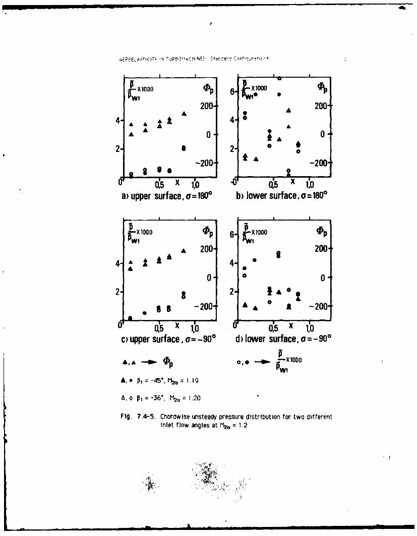
;4EPIELA ;TICITY iN 'jP501-';4i'H'NF- :tqr ,j-iC

X 10 0 0 P 6 0 0OA 0- A 200-

4 A LA 4- 0A A A A

0

-200 f A& -200-2 0

0 OR 1,0 01,(5 X 10a) upper surf ace, a= 1800 b) lower surface, (y180*

PtA 2001 O1 200-4 k 4- *

0 0 0

* s-20 1 0 i -200-

0 5 x 1,0 0,5 x 1,0c) upper surface, a= -90* d) lower surface, (y 90o

A, A -- W 0 ,0 -- IN- WE-XIaOO4)P PWI

A,. p,-45". r12I 1.19

A, o0 -36', l12,5 1.20

Fig. 7.4-5. Chordwise unsteady pressure distribution for two differentinlet flow angles at M2 1 I.2

EPRF-Lausene, LABOPATOIRE DE THERMIQUE APPLIQUE E T DE TURBOMACHINES I

2

. . .. . . .. . . .. . . . . . .. . - - --- - - - - - -

.

a............ --- 11 -------- -------- 370.....1

c). chie.n.pctre.ro.a.in ar.es facility.../2./................ .... l.

F~g.7.4-. Tie-avragd flw fo t$,1 .

x ''

AEPOELASTICITY iN TUREOMAChiNE. Standard Configurations 112

a change in incidence angle will influence the unsteady response closer to the

leading edge

Care should still be taken when comparing the ampl'tude of the unsteadypressure coefficient, AEp This coefficient, as can be seen from eq. (3), is

normalized with the steady-state dynamic pressure (p. - 51), which is

dependent on the inlet flow angle.

Integrated values

The number of pressure transducers on the blades (6 on the suction surface, 5on the pressure surface) is not enough to determine the blade force and

aerodynamic damping coefficients accurately. However, as long as theunsteady pressure response along the blade is smooth (see for example Fig.7.4-4) the trend of the integrated values should be correct although themagnitude will be inaccurate, depending especially on the pressure responseclose to the leading edge.In Fig. 7.4-7a the aerodynamic damping coefficient is presented as a function

of the interblade phase angle for two different inlet flow angles. For an inletflow angle of -100 the tests have been performed with a variation of 180

interblade phase angle. The aerodynamic damping coefficient is representedtogether with the experimentally determined 95% confidence interval (seeAppendix A4). The sinusoidal shape, as also seen for the first and secondstandard configurations, is recognized, although with some higher harmonics.It is concluded that the cascade shows instability for some interblade phaseangles at an outlet Mach number of M2i3=0.9.

In the same diagram the four interblade phase angles defined as aeroelastic

test cases (00 , 90* , 1800, 2700) for a -450 inlet flow angle are presented.Also at this flow angle the cascade shows instability in the region of a 2700interblade phase angle.The same sinusoidal form is also recognized for other outlet flow velocities(Fig. 7.4-7b). Here it is also noted that, as already seen in Fig. 7.4-7a, thecascade is unstable, in subsonic flow, for interblade phase angles around 2700

(=-90°). However, for a supersonic outlet Mach number of M2i 1 .19 theaerodynamic damping coefficient indicates instead a stable blade vibration at

this interblade phase angle. This phenomenon which is also present for other

flow angles, will be discussed at the same time as the local blade surface

pressures

Up till now, only two methods (NO 10. semi actuator disk theory; NO 7, finiteelement, potential flow) have been applied to calculate the aerodynamic

.t . r1 -

EPF-Lausnne, LABrPATGlPE DE THEPMIGUE APPLIQUEE ET DE TUPBOMACHINES II 3

12

,I\

\ x

0 stable

"unstable \\ ,

S:i: -"450-12 -

0 180 360o(0)

a) Aerodynamic damping coefficient for two different inlet flowangles at M2=O.90.

12'- I - : M2 = 1. 19& : :M2 =1.02+ : M2 = 0.90X :M2 0.76

+stable + C : M2 = 0.580 unstable

-12-0 180 360

G(0)b) Aerodynamic damping coefficient for different outlet isentropic Mach

numbers at an inlet flow angle of -45"

Fig. 7.4-7. Experimentally determined aerodynamic damping coefficientt

AEPOELASTICITY IN TURBOMACHINES: Standard Configurations 114

damping coefficient. These results are given in Fig. 7.4-6, together with theexperimental data (including 95% confidence interwals) for the 8 aeroelastictest cases selected. It can be seen that, by comparing Fig. 7.4-8a and c, theshape of the aerodynamic damping coefficient versus the interblade phaseangle is similar for both theory and experiment. The results of Method 7 andthe data agree well, apart from at ==9o. However, the maximum dampingvalue is not reached at the same interblade phase angle for Method 10, andthe predicted results for this method are one order of magnitude larger thanthe measured ones.The experimentally determined aerodynamic damping coefficient versus theoutlet Mach number, for g=-900, agree well with the results predicted byMethod 7 (Fig. 7.4-8b). However, the shape for Method 10 does not agree withthe data (figs 7.4-ab,d).Although the order of magnitude of the damping coefficient is the same forboth the Method 10 and the experiment, the theory predicts a stable vibrationfor subsonic Mach numbers, whereas the experiments (and Method 7) indicatea stability for the supersonic Mach number instead. At present the reason forthis discrepancy is not clear, and the author of Method 10 believes that theeffect of blade camber in the semi-actuater disk theory should be validated1561. Obviously, an inaccuracy in the experimental results cannot be excludeda priori but the experimental data agree well with results from Method 7 , soit is probable that the experiments are correct in trend and order ofmagnitude of the aerodynamic damping coefficient.The reason for the discrepancy between experiment and Method 7 at 900interblade phase angle is found by examining the local blade surfacepressures, and will be discussed in that section.

,:oA '~=I II ~ Ii I

EPF-Lausenne, LABORATOIRE DE THERMIQUE APPLIOUEE ET DE TURBOMACHINES 115

C .07411 c .0744

y a .76 1T~ .764t 7 56.6 r - 56.6

H, .28 M,-3 .19

I 1,. -,s. - 1 I - ..

". .. ......... tIMI M 4 I 0 .0.90 .IM

METHOD, 7 2 ETHOD 7k . -71. -0

IN,

u 942. w: 942.o - " 1 .115 -k

a 60.4 8 60.4

0 ________ 0 I I a 904

FS UN " ' " / STALE D LIS.K0 -4 , USTABLE' STAB0L[

8.0. . . . . . .-- 6.0

r M2

PLOT 7.4-6.21 FOURTH STANOARO CONFIGURATION CASES,3.6-@ PLOT 7.4-6.1, FOURTH 5TANDAR CONfICURATION CASES -7EPFL-LT 60 AEODYNAMIC WOK 680 DAP PING COEFFICIENTS EPFL-LTr 60 AERSOTNAMIC 6ORK AN OR PING COEFFICIENTSSS20-2 IN SEPENOANCE OF INTERBLOCE PHOSE ANGLE 5530-1 IN OEPENO6NCE OF OUTLET ISENTROPIC NACH NUMBER

a) b)

Experimental data (with 95% confidence interval) and predicted results.-100,,

method:10 (M2 is=0,9 ) method:10 (a -900)

II

I I

~~A AAA

I I

+100 I I

-180 0 0 +180 0 0.5 1.0 M2isl.5C) Predicted (Method 10) d) Predicted (Method 10)

Fig. 7.4-6. Experimental aerodynamic damping coefficient togetherwith predicted results from Methods 7 and 10.

AEPOELASTiCITY iN Li PB0MACHINES: Stindarc Co 1furaoion 1 1

Blade Surface Pressures

Theoretical results from one method (NO 7) have been obtained for this

standard configuration. In general, data and the predicted results agree well

(Fig 7.4-9), both as regards the amplitude and the phase angle of thepressure coefficient cp(x,t) along the blade chord.

The experimental accuracy, represented in Fig. 7.4-9 as a 95% confidenceinterval (see Appendix A4), shows as expected that the uncertainty in themeasured phase angle is greater when the pressure amplitude is smaller

Considering this confidence interval, the data and the prediction agreeextremely well for the subsonic cases (Fig. 7 4-gab,c; compare Fig. 7.4-2a,b,c for steady-state blade surface distribution) at -900 interblade phase angle.This is true for both the amplitude and the phase angle.

Especially interesting to note is that the trend is correct for all cases. Onthe pressure (upper) surface of the blade the only notable exception is thefirst pressure transducer (x=0.l) which indicates a low pressure amplitude,whereas the theory predicts a higher value here.

Towards the trailing edge (last transducer at 84% chord) both theory andexperiment predict an increase in the unsteady pressure amplitude on thepressure surface, The value here approaches the magnitude of the pressureamplitude around the 20% chord on the blade suction surfac( . This canpossibly be explained by the fact that the last transducer on the pressuresurface and the second on the suction surface are both situated in the vicinity

of the throat (see Fig. 7.4-1b), and that the aerodynamic coupling effects aretherefore high It can also be seen that the phase angles in these twopositions are fairly close together (e.g. #i us (x=0.14) = +1700 , *plS(x=O 24)

+ 1600 in Fig. 7.4-9a).

The same conclusions can also be drawn from other phase angles, as long asthe flow is subsonic (Fig. 7 4-9f,g,h for 1800, 900, 00 respectively), apartfrom the phase angles with in-phase blade motion (Fig. 7 4-9h). In this lastcase the experimental and theoretical results show instead a discrepancy of

the order of 900 or more, and the experimental data on the suction surfaceshow some fairly large irregularities. The phase shift of 1800 between thetwo pressure tranducers located at x=0 24 and x=0.44 is particularlyinteresting. The same phenomenon is found also for all other inlet flow angles

and outlet flow velocities investigated [231, but no explanation for this hasyet been put forward However. it should be noted that the unsteady pressuresignals at @=04 are weak, and the confidence interval is large for almost allpressure transducers

S-A I m III II I _

- - tjsrr e L A I2,E I, PE DE THEPMI1iIE APPLIQUEE ET CE TIPBO iACHINF-- ii

"The re:' t ' f the differece in 3erod'4r, anllc damr'p ing coefficient between

experiment and Method 7 at q=9W0, as found in Fig 7 4-8a. can now be

e:pIained on the basis of Figs.7.4-9. It is here seen (Fig 7.4-9g) that the

theory predicts a somewhat higher pressure value along the whole suction

surface than the experiment for this interblade phase angle. The phase angles

are predicted just as well for g=900 as for other phase angles, wherefore the

difference in Z" can be attributed to differences in the pressure amplitude

However. no explanation for why the difference in tp(US) between experiment

and theory is larger for v=90 ° than for other interblade phase angles is

presently put forward.

As the back pressure is lowered towards transonic and supersonic outlet

velocities the unsteady pressure amplitude and phase angle on the pressure

surface do not significantly change from the result in the subsonic cases (Fig.

7.4-9d,e). On the other hand, larger differences are notable on the suction

surface.

First of all it is concluded from Fig. 7.4-2d and 7.4-9d that the transition

from subsonic to supersonic flow on the blade suction surface (x=0.45)

introduces a phase shift in the unsteady pressures for a transonic outlet

condition (Mzis=1.02) at a -900 interblade phase angle. This shift is present

both in the experimental and theoretical results, although to a larger extent

in the experiment. Aft of the sonic transition the theory indicates an increase

in the unsteady pressure amplitude, which is not seen in the experiment.

Towards the trailing edge both the theoretical and experimental pressure

amplitude increases probably due to the presence of a shock wave, although

not on the same scale. It should however again be noted that the last pressure

transducer is situated at 84% chord and the experiments indicate that the

shock at an isentropic outlet Mach number of M2 i,=1.02 is situated somewhat

closer to the trailing edge (Fig. 7.4-10).

Again, as in the subsonic cases, the experimental increase in pressure

amplitude towards the pressure surface trailing edge is larger than the

theoretically determined one. The pressure surface phase angle (4p63 ) is,

however, well predicted (Fig. 7.4-9d).

- ,a-I

- ii i I iiiiI I I I I

118

"__ _ _ _ _ _ _ c .0744 c .0744

7 Ti .76 7 i .76

. ...5 6 . 6 7 - ' 7 . 5 6 . 6

f A - - - D P2

MI .19 MY .26

STTMOIJIUTTNiINN 1.Mi .58 RIM 1ROUSIC ~ ' 2 .76

. T - METHOD , 7 2 -7 1 . 40.0 E NER D .o , , P.

hi: .0019 11-.0019

30.0 1 h1 .0033 30.0 h .0033

0i 942. ? i 942.1, 00.0 . . .- . B - .27 20.0

I, .1 rk 1- .. . .,

8 6a . 8- 60.4

10.0 10. 4-8 0.I -90. OD -9o.1 +: ' -le .:-7eo

.00

-. . ~ , o• - __ -- ,- --

PLOT to-U *USTABLE .0 .SE

-90. -90. -AD. 1 )0 - - 90.

S. UNSTALE" NSTABLE

-,I8.0. -lA. ' ' + I I UIR*LN"

0 .0PLOT 7.-2., FOURTH STANDARD CONFIGURATION CASE i I PLOT 7.-..2, FOURTH STANDARD CONFIGURATION CASE , 2

MAGNITUDE AND PHASE LEAD OF UNSTEADY BLADE MAGNITUOE AND PHASE LEOAD rF UNSTEADY BLADE

SS3D-I SURFACE PRESSURE COEFFICIENT. SS3C-I SURFACE PRESSURE COEFFICIENT.

a) b)c O~I c .0744

7 Ti .76 r .767 56.6 MS7- Z . = 56.6

. US DATA Y ai -I 0. -T- -

MI .28 M, .29W"" " ", -44. 5 - ""t,-44.5

........................ I i.MR....TU. .IN

T-- -C O G R T I T N U REl R "- M , . 9 0 $ T., oN N, O C O NFI CA A A ANM , A 2 l .1 .0 2

40.0 METHOD, 7 P2: 71. T0.0 R OEDMI0 7 P, -71.

hB, .0016 h, .0016

3 0 .0 h T i , 0 0 2 9 3 .o h , .0 0 2 9

.. 942. c, 20•0 u 942.

I 8 .160.4 *0.0 8 -10: . 41,=.. DO_ 0.

4 i T O -91. a -90.

Edi .17 d .17• , , 11 '=i:1 a,: ,o• Ti ' ?i , ,,I T A•A i80. : rd) - -180.STABLE STABLE

-90. 90. AD - -- --.- -A0.0UUNST LE*

. NSTABLE"

-1eo. .o= k I.C.°° -180. €o " ' : ::( .80"

P .4-2.3, FOURTH STANDARD CONFIGbRATION CASE * 3 PLOT 7.4-2.4, FOURTH STANOR CONFIGURATION CASE , 4

MAGNITUDE AND PHASE LEAD OF UNSTEADT BLADE A GNITUDERANO PHASE LEAD OF UNSTEAOT BLADE

SSA- SURFCE PRESSURE 0EFFICIENT. SUA-I SURFACE PRESSURE COEFFICIENT.

c) d)

Fig. 7.4-9. Continued on next page

IPF-LaU38nne, LABORATOIRE DE T3IERNIGUE APPLfcuEE rT DE TURBOr1ACt1INE 11'4

I A .0714 . 0714V .7 .76

Mt- y156.67 56.6

P, M, 16 --- .1 2

9 P1. -44.5'HA - M2 ~ ~u .90

40.0 - E ANCT 7 P2 -340.0 - off RH 7 P2 1 -71.6".01 h.. .0016

30.0 - ,. .0033 30.0 it, 9, .0029

200~~ 1 9242. .1 0.0 -4 * . . .u 94Z.20. A .09 A .2

5 a 60.16 a 60.14101 -g0. - 1 80.

Af IS 1*17ISI .

so.. 90. . . . . . .90.

-s.2 90 -0. . .7

TAUNSTAB.E"

-1n80o~. P -to . -10 '-IS

0 0 .0kS

PLO 7..25, OUTH TADAR CO I~MTIN ostI * PLO FORT 1WI*W'S COFIURTIN AS

.76 300 ..011*6. 6.6 '56.4

TA92. *6 0 -S9AT9M2S1 -9 - M, .9

30.0 1 AT .0029-.P0 93 33h90C9T0910 93 .002

0 0909 w9 s93 $120 20. 9942.g~91101 9 90troo 9tlo to3029-3 aUFC 12339 .9P129. 999 31F91P121 eIrCro

a) 2 04 )6.Fig. 7.4-. Untaybld ufcepesr.cefcet0o h

aeoeas d test cae7vria asth aapitinct .5 .. onidne.ntrv.

AEROELASICITY IN TURBOt1ACXINES Sta..tlro Corifioura,'Insf

n BLAOE 2

B :LADE 3: : :

Ca :BLADE'd

------ ---- a----a

0.0 1.0X/S

Fig. 7.4-10. Flow throughi the cascade at an isentropic outlet Itchnumnber I 2,,z.02 In a linear test facility /25/.

EPF-Leusanne, LABORATOIRE DE THERMIQUE APPLIQUEE ET DE TURBOMACHINES 121

As the back pressure is lowered (M2is=1.2, Fig. 7.4-9e), the experimental and

predicted results still agree well on the pressure surface. This is also true

for the suction surface, upstream of the shockposition (xshock=0.5, see Fig.

7.4-2e). However, for this outlet Mach number, contrary to test case 4

(M215=1.02), the experiment shows a larger influence of the shock on the

unsteady pressure amplitude than the theory. Furthermore, the suction surface

phase angle (*,i3) snows some discrepancies between theory and prediction

aft of the shock.

As seen in Fig. 7.4-Ba the cascade configuration showed an instability at high

subsonic Mach numbers at #=-900, whereas other interblade phase angles

showed stability. The reason for this change of sign in the aerodynamic

damping coefficient can be found by investigating the unsteady blade surface

pressures for g=-900 and 5=+900 at an outlet Mach number of Mzis=0.90 (Fig.

7.4-9c,g). It can be seen that the experimental blade surface pressureamplitudes (Ep) are similar in both cases. Case 7 (w=900) is stable mainly

because the forward 60% on the suction surface are stable. However, case 3

(g=-90 ) is unstable as the whole suction surface is unstable.

No physical explanation for this change of stability can presently be given.

It is also interesting to note that the two last pressure transducers on the

suction surface indicate almost the same amplitudes and phase angles for 6=-

900 as for 5=+900, and that the first four suction surface tranducers change

at an almost constant value with the variation in interblade phase angle.

(6pi1pi3(5=+90°)-4pi3(5=-90 ° ) = 620, 550, 710 and 71, resp., see Figs. 7.4-

9cg and data sheets in Appendix A5, section 4.). The same trend can be

recognized from the prediction model 7 for x<0.6. Aft of this position a larger

difference is found in Pl3 between theory and experiment. A possible

explanation for this phenomenon could be the hypothesis of a small separationbubble on the last 30% of the suction surface at M2Q,=0.9 [281.

From Fig. 7.4-8b it was also concluded that the cascade configuration became

stable with an increasing Mach number. Once again, the reason can be found by

investigating the unsteady blade surface pressure distribution (Fig. 7.4-9c,e

for M zis=0. 9 , 1.2 resp.).

It can be seen that the pressure surface data are identical for both Mach

numbers. However, the suction surface pressure amplitude and phase angle

are different at x=0.5. At M2is=0.9 the phase angles indicate instability at

x=0.5, while at M2is=1.2 the same transducers instead show a high stability

($plS=-90i). This change in stability can thus clearly be attributed to the

presence of the shock at 50% chord, and it can be concluded that the shock

has -a stabilizing effect, at least for low supersonic outlet flow velocities.

4'I

-F,' .• b.

' - mbIIIIIII I •II II I I

AEROELASTICITY ;N TUREOrIACHINES: Standard Confiourations 122

Conclusions for the Fourth Standard Configuration

From the controlled excitation study in traveling wave mode (i.e. constantinterblade phase angle between all blades) on a 17% thick, 450 camberedsteam turbine cascade, experimentally investigated in an annular test facilityin subsonic and supersonic flow, it can be concluded that:* The fact that the unsteady experimental data and the (by Method 7)predicted results agree well validates mutually both approaches, at least for

shock-free flows.* Prediction model 7 gives a good overall view of the unsteady bladesurface pressures for subsonic outlet flow conditions. In the transonic andsupersonic cases some discrepancies between the experiments and theory canbe found in the vicinity of the shocks.

Conclusions for aerodynamic damoing:

* The experimental date indicate a slight instability at subsonic outletMach numbers (for g=-900), and stable vibrations for supersonic outlet flowconditions. This behavior is predicted by Method 7 but not by Method 10(semi-actuator disk theory) (see Figs. 7.4-7, 7.4-8).

Conclusions for unsteady blade surface pressures:

* The local unsteady blade surface pressure coefficient on the upper andlower surfaces is well predicted by Method 7 for subsonic flow conditions,especially by considering the experimentally determined 95% confidenceinterval (Fig. 7.4-9). The only noticeable exception is the first transducer on

the pressure surface, located at x=0.101.

* Also for supersonic outlet flow conditions, the experimentallydetermined unsteady pressures on the upper (= pressure) surface are predictedwell, both as regards amplitude and phase angle (Fig. 7.4-9d,e).

* Some discrepancies between the unsteady pressure data and predictedresults exist on the suction surface for supersonic outlet Mach numbers (Figs.7.4-9d,e). Here, the unsteady shock impinging on the blade suction surfacedoes not appear in the same way in the theory and the experiment.* The change in stability at approximately sonic outlet conditions can beattributed, both in the experiment and in Method 7, to a change in the localunsteady blade suction surface pressures in the vicinity of the shock.

ILI

EPf-Lausanne. LABORATOIRE DE THERMIOUE APPLIOUEE ET DE TURBUCIACHINE5 13

7.5 Fifth Standard Configuration (Compressor Cascade in HighSubsonic Flow).

Definition

This two-dimensional subsonic/transonic cascade configuration has been

tested in a rectilinear cascade air tunnel at the Office National d'Etudes et de

Recherches Arospatiales (ONERA). The configuration and experimental results

are included by kind permission of E. Szechenyi ([29-311).The cascade configuration consists of six fan stage tip sections, each blade

with a chord of c=0.090 m and a span of 0.120 m. The maximum thickness-to-

chord ratio is 0.027, with no camber and a gap-to-chord ratio of 0.95. The

present configuration was measured with a stagger angle of 59.3 °

The cascade geometry is given in Figure 7.5-1 and the profile coordinates in

Table 7.5-1.The two center blades can vibrate in pitch about several axes, and then the

aeroelastic coefficients for different interblade phase angles can be computed

by linearized summation of the unsteady pressure responses on all six blades.

Experiments have been performed with oscillation frequencies between of 75

and 550 Hz, inlet Mach numbers of between 0.5 and 1.0 and with incidence

angles between attached and fully separated flow (20 to 150).

Both the time-averaged and time-depencent instrumentation on this cascade

is extensive and a large amount of well-documented data has been obtained

during the experiments. The large number of flush-mounted high response

pressure transducers on one blade (9 on lower blade surface and 10 on upper

blade surface) allows the determination of resultant time-dependent blade

forces.The upstream and downstream steady-state flow quantities are determined 2

chord lengths upstream of the leading edge plane and 0.5 chord length

downstream of the trailing edge plane, respectively.The unsteady pressure measurements are all filtered, simultaneously sampled,

multiplexed, digitized, averaged over a certain number of periods and recorded

on disc after which the pressure, lift and moment coefficients are computed

[291.

-- s, ,+

AERGELWICITY IN TLURBOrACMMtES. 1anjar'

cascade leading

High Subsianic CrMiMSua PECofI2 edg pan

A suct i surfa esue surface-

Visration nupitche)d(,g)=(.,.

d + tikes/hr) .2

edge0.2m Ol oe ade vbae

M1 = 0.ar2a ide (0.5-1.0) 755WHz

Working fluid. Air

Fig. 7.5-1. Fifth standard configla'tiorl Cascade geometry

EPF-Lautl3nne, LABORATOIRE VE THERMIQU[ APPLIOUEE fT VE TURBOMACHINE5 125

c 0.090 m

Upper surface Lower surface(Suction surface) (Pressure surface)

xy y

0. 0. 0.0.0124 0.0016 -0.0016O.0250 0.0018 -0.00180.0500 0.0026 -0.00260.0750 0.0033 -0.00330.1000 0.0041 -0.00410.1500 0.0053 -0.00530.2000 0.0062 -0.00620.2500 0.0079 -0.00790.3000 0.0101 -0.01010.3500 0.0103 -0.01030.4000 0.0111 -0.01110.4500 0.0119 -0.01190.5000 0.0124 -0.01240.5500 0.0128 -0.01280.6000 0.0133 -0.01330.6500 0.0135 -0.01350.7000 0.0135 -0.01350.7500 0.0128 -0.01280.8000 0.0116 -0.01160.8500 0.0098 -0.00980.9000 0.0076 -0.00760.9500 0.0048 -0.00481.0000 0. 0.

LE radius TE radius- -= 0.002c c

Table 7.5-i Fifth standard configuration Dimensionless AirfoilCoordinates

i1

AEROELATIC:TY IN TIURBO ACHINE. 5tandard Configurations 126

Aeroelastic Test Cases

A large amount of data has been obtained durinq the tests [31., Of this, 29

cases were recommended as test cases in [41

Of special interest in this fifth standard configuration is the extensive

variation of time-averaged parameters, such as inlet flow velocity (MI ) and

incidence (i).

The inlet Mach number is varied from MI=0.5 to MI=1l0, and the range of

incidence is from fully-attached (incidence less than 50) up to fully-

separated (incidence greater than 100) flow conditions.

At the Cambridge Symposium [31 it was concluded that the present state-of-

the-art of prediction models does not allow for the calculation of stalled

flow (7]. Therefore, the 29 recommended cases from [41 were reduced to the

ones dealing with attached flow only. A total of II test cases were then

selected. These are contained in Table 7.5-2.

Time Averaged Time Dependent Parameters FlowAerolastic MI i P21Pwi a a f k

Test Case No. (-) () (-) (rad) (0) (Hz) (-)

1 0.5 2 0.84 0.00524 180 200 0.37 Attached2 4 0.86 " "

3 6 0.87 Part. sop.4 4 0.86 75 0.14 Attached5 " 125 0.22

6 -" 300 0.547 " 550 1.028 6 0.87 " 75 0.14 Part. sep.9 " 125 0.22

10 -"300 0.56

I I 550 1.02

Pitch axis at (x, ya) = (0.5, 0.) for all the above aeroelastic test cases

Table 7.5-2. Fifth standard configuration.

11 recommended aeroelastic test cases (restricted set from /4/)

EPF-Lausanne, LABORATOIRE DE THERMIQUE APPLIQUEE ET DE TURBOMACHINE3 127

Discussion of Time-Averaged Results

The 11 proposed aeroelastic test cases comprise three separate stationary

flow conditions, all at the same inlet flow velocity ( 11=0.5), but at different

incidence angles (i=20 , 40 and 60, respectively).

These data are presented in Fig. 7.5-2, together with the theoretical results

of Methods 2 and 3. The data and the theoretical results agree well, if the

theoretical incidence is slightly modified. The theoretical incidence angles

for Method 3 in Fig. 7.5-2b,c are itheory= 2 .50 and 4.0 ° , compared to the

experimented ones (and theoretical for Method 2) iexp=4.0 and 6.0 ° ,

respectively. This change in steady-state incidence angle corresponds fairly

well with the change introduced in the first standard configuration for

similar reasons (&i=2.30 to 40 in standard configuration I; Ai=1.50 to 20 in

standard configuration 5).

It should also be noted that the theoretical results obtained using Methods 2

and 3 agree extremly well for the same theoretical incidence angle (Figs. 7.5-

2a, b for itheory=20; Figs. 7.5-2b,c for itheory=40).

It is thus likely that an experimental effect, which is not taken into account

in the inviscid theoretical flow models, is responsible for the need to correct

the experimental incidence angle in order to achieve a good steady-state

agreement.

The largest discrepancy between the experimental and theoretical results is

found on the suction (=upper) surface in the leading edge region. This effect

becomes more pronounced with an increase in incidence angle. It is found that

the difference in the leading edge region between Method 3 and the

experimental data is somewhat larger for the present cascade than for thefirst standard configuration (Fig. 7.1-2). This can perhaps be attributed to the

higher flow velocity and the sharper leading edge in the present case.

However, calculations with other methods should be performed before any

detailed conclusions regarding the reasons for this discrepancy can be drawn.

AEROELASTICITY IN 7UPBOY'A.C)INE. 5tandrd C.urtr or: ."

C,.0901 C- c 090"7 . .95 T:.95

59.3 7:59.3M - . .,M2 M - P

I •, N2 A -

C] .US DATA Y.a - M -US DATA - .A -

..... ....-............ DO" 23h" " *L

/ DATA... - .LS D.ATA ,, 1 * .5

...............N .. I t s c3 A25 h -.-IA .... S - -l~l0 : I h

t-E VD. 2E*E 002l

IIT IhT

ATS , (1,

-r IJ -8 - 8 -

- .* d:.027 .2S- ,- - ' .27d , 027

-p . --.--- :.- : : : D.: -

a Cs . o. I I.

PLOT 7.-1.21, FIFTM STANOARD CONFIGURATION. CASES 2.4-7. PLOT 1.5-Il, FIFTM STANDARD CONFIGURATION. CASE I.TIRE AVERGED ALROE SURFACE PRESSURE TIRE AVERAGED BLADE SURFACE PRESSUREDISTRI UTION FOR AI-O.S AND INCIDENCE-4 DEG. DISTRIBUTION FOR MI-O. AND INCIDENCE.2 DEG.

a) b)

_________ T.95759.3

C3 -u I.UDATA pa Y.X LS DTA M'' .5 Fig. 7.5-2. Time-averaged blade

1P -65.3

,, , surface pressure distribution for- - - ip= 20, 40 and 60 , respectively.

Ca5

x x : .027

0. I

PLOT 7.5-I.3 FIFTH STARNOAR CONFIGURATION. CASES 3.0-11.TIRE IVERARGED St ACE SURFACE PRESSUREOISTRIBUTION FOR RI.O.S "D INCIAENCEo$ DEG.

c)

CPF-Leu3sanne, LABORATOIRE DE THERMIQUE APPLIOUCE ET DE TURBOMACIIINE5 129

Discussion o'f Time-Dependent Results

Up till now, four unsteady prediction models have been applied to the fifthstandard configuration (Table 6.1). From the results, both the time-dependentblade surface pressures and the stability limits of the cascade can beevaluated.

When comparing the unsteady results it should be considered that theexperiments were performed with only one blade vibrating (i.e. only theinfluence of the blade on itself was considered), and that aeroelastic couplingeffects between neighboring blades has not been corrected for. This isunfortunate, but the objective of the experiments was to investigate flutterat high incidence angles, for which the aeroelastic coupling effects have beendetermined [311. It was only because it was found that present predictionmodels cannot treat such flow conditions that the low incidence angleexperiments were selected as test cases.

In order to estimate how large the aerodynamic coupling effects are, abreakdown of the theoretical results obtained from Method I has been done.This study shows that if only one blade is vibrated (in Method 1), the results

approach the experimental values. This fact will be discussed in the followingsections.

Integrated Parameters

The experimentally determined aerodynamic damping coefficient (one blade

vibrated) and the predicted results (all blades vibrated) agree well for anexperimental incidence angle of iexp=60 (Fig. 7.5-3a), over a wide range ofreduced frequency (0.22<k0.02). However, the agreement is not so good for

iexp=4 ° (Figs. 7.5-3b,c), althougq the stability trend is again correct.The same information is found by examining the moment coefficient (Figs.

7.5-3d,e,f).It is presently not possible to explain the sudden change in the experimentalcurves around iexp=40 (Figs. 7.5-3c,f).

ACRO!LAITICITv IN TURrOMCHINrn. 31axaro conflguiat1ons 1 3o

A certain discrepancy is found also for the different theories The flat platetheory (Method 1. Itheory=Oo.) and Method 2 (ltheorv=lexp, full blade geometry

taken into account) agree well, whereas Method 3 (full blade geometry,itheory=2 5 and 40 resp in Figs. 7.5-3a-f) is somewhat nearer to the

experiments. It is found that the difference is largest for the magnitude andthat all the predicted phase angles *m are close to the measured ones.The reason for the differences between the theoretical model predictions arenot apparent at the present time.The aerodynamic coupling effects can be estimated by considering thedecomposition of the results of a calculation with all blades vibrated, intothe separate influence coefficients of each blade [28. 30. 591. Thisinvestigation, based on results obtained from Method I (flat plate, itheory=0 °),is shown in Fig. 7.5-4 for a 1800 interblade phase angle. It is concluded that,for w=1800, the amplitude and phase angle of Em(x,t) does not change if 2 ormore blades are vibrated. However, a certain change is found if only one bladeis oscillated. In the present case the amplitude and phase angle of a single-blade vibration are Em= 1.24 and #m=-250, resp., whereas the corresponding

C. .090M , -I , .agoJ7 . ro.95 .J AS.95

7 59.3 7:59.3MI, . 5 ._M 2 , .5 M, x,.5C. -US DAT M2Il =SORII • "

k , 0. 0 - DT 0. Y 0.X.-LS DATA -I 0. X-LS ATA, M10, 0.5"' -6S.3 P, -63.

SII0+ -DATAI M, OA TR M2

C l I OT

METHOD, I 0 - ME__ THl D, I i -

-4 -. . P-6 -4. - A2.. ...... ......... MEt0O0 = 3 h.I h - ................... METHOD: 3 1=250 h, , -

ITT, - hT

-

: .0052 =: .0052

a), : --2. k o -2. -ok : -

6o 8 :-o 180 . .a 180d o .027 1 d ,.027 |

-. : st UNSTABLE c UNSTABLE

S2. . .2.

0. 0.5 1 0. 0.

PLOT 7.S-6.3, FIFTH N50DR0 COFIGUAR';O . CASES 0-Il. PLOT 7.5-6.2, FIFTH 5TA0N4 CONFIGURATION. CASES 4-7.AO0OrOM IC OR AN0 0A0mIG COE0FICIENTS AERODYNAMIC ORK 4N0 DA PING COEFFICIENTSIN OEPEA0OG CE OF REDUCED FOEOUEACT IN 0EPENOANCE OF REDUCED FREOUENCV.

a) b)Fig. 7.5-3. Continued on next page.

EPF_-J~Ar-e. LAOPATOR DE TMHRMOUE APPLIOUEE ET DE TL1REt1ACHINE5 ,i

€,090M ago" .090M

7 T.95 ______. t.95

T 59.3 59.3

TO -U DATA5 02 0. 0.15 DATA .3- M

, 0.5 02 0.5

SNCCLm ht LS DIAT 1N XST-0A -M2oDA T.

. K A2, - .... .-O~- AE DTADD 2 0M2_

h. .- .. - - METO.. . 2 P2 20.N i - 2. 1 -

.0052 If.00521a o 2257 0. 10.

80 180.027 - d .027

S. STABLE -ISO.

• . : ; ; ' : : ) I I '-180. p . : :-0. ,20, . o. o ,.

ILI' - F IFTH STANDRD CONFIGURATION. CASES 1-3*EXTRA. PLOT 7.5-S.0 s FIFTH STANDARD CONFIGURATION. CASES 8-1I.AEROTNARMIC WORK AND DAMPING COEFFICIENTS AERODNARMIC MOMENT CEFFICIfN/ 0 OA S 5ELIN OEPEORNCE OF INCIDENCE ANGLE. IN DEPENDANCE OF REDUCED FRE N CT -

c) d)'Sc c.N..l91 090"

.95 p . T :9 1'. .9 5

S:59.3 7M, PI X . : .5 .,

C3 -US DATA . 0. 0 U 5 DATA to 0.P2 PI ,0.5 - 0.5

X -S DATA, - . X -L5 DATA.I-6 3

.3

20. _METH E O, 1 4.0 P 20.- - - -. ETHOI! 2

E 00 2 1- bT INT, -... ....... METHO . , -=2 -

s .0052 .0052

. 10. U 0- . w 1257

k- k .37so- 5i-

180 180

d .027 d~* .027A0. I

UNSTABLE

-90. .90.1~4 _

0. €.- ' -- & - D. -€ 4,

.1- .D. -

TD 0. . 0. I~ 20.

PLOT 7.5-521, FIFTH STANDARD CRNFIDUATIRN. CASES N-7. PLOT 7.5-5. , FIFTH STANDARD CONFIGURATION. CASES I - x. TAERDOTNARIC N AEN C EFFICIEAT AND PAASI LEAD 0ERODINA i[ MOMENT COEFFICIENT ND '1A5E LE0IN DEPENDANCE OF MEDUCED I MlEUEMCT. IN OEPENODANCE O

F INC IDENCE ANGLE.

e) f)Fig. 7.5-3. Aerodynamic damping and moment coefficients for the

fifth standard configuration.

AEROELASTICITY IN TURBOMACNINES: Standard Confiqurations 132

values are cm = I 58 and 4m=-230 for 6-4 blades viorated (Fig. 7 5-4) The fact

that the phase angle does not vary with the number of vibrating blades is

clearly the reason for the good agreement for the phase angle (#m) between

the experiment and the theory in Figs. 7 5-3d,e,f. The study indicates also

that, if all blades were vibrated in the experiment, the experimental 6m value

would probably be somewhat larger than the ones prespnted, and thus

approach the theoretical curves in Figs 7.5-3d,e,f.

Blade Surface Pressure Differences

As the blades in the fifth standard configuration are thin (2.7%) it is of

interest to evaluate and discuss the blade surface pressure difference

coefficient AY(x,t-). This parameter is given in Fig. 7.5-5, for different

incidence angles (iexp=2, 40 and 60) at a reduced frequency of kexp=0. 3 7 .

It is concluded that, for iexp=20 (Fig. 7.5-5a), the phase angles (#6p) of the

pressure difference coefficient in the experiment and in the different

theories agree well. A certain discrepancy exists, however, in the magnitude

(A,). Methods I and 2 predict identical values, whereas the experiments

indicate lower pressure difference amplitudes along the whole chord. This

effect becomes more pronounced in the forward part of the blade for larger

0.6- MOMENT COEFFICIENT

CONTRIBUTION OF EACH PAIR

OF BLADES

REFERENCE BLADE :0

0.0 ..............-NUMBER OF BLADES =64em

or* ble Several blades

-0. 6 On blade ... --vibrated vlibated

* :SIGMPISO0.

-h 2 p

0.0 0.8 R m 1.6 2.4

Fig. 7.5-4. Aerodynamic coupling effects for o=1800, with the number

of blades as parameter ( 64 blades used for the

decomposition)

133

Y 59.3 759. 3

A C3UDAAV6, 0. PIT a.-US0585 y0.

01,. -63.3DAT I M. ,c~os a 2. .SICT I ..Wc5~ * -DATA

OOS2 .0052

k s.37 k .37

Al .027 d .027aIS

*ISTSTE

090

SaSS.

II 10. -so. 1 : : :-

0. S 0

PLOT 7.5-3.1. FIFTHI STANDARD CONFIGURATIO.S 1. PO .-.. FFHSTRAINO NFGRAINSCSEMAGNITUDE AND PHASE LEAD Of SLADE SURFACE MAGNITUDE AND PHASE LS I' 0 S LADE SURFACEPRE SSURE a IFFEREMCE COEFFICIENT. PRESSURE DIFFERENCE CO"EPITET.

a) iexp=20; k ex -.37 b) I x 4 0 ; kxpO-.37

o090"_________ r.95

Y Sa9.3

C3LS ATA 1 0.

6~ Fig. 7.5-5. Blade surface pressureT20' . 0 difference coefficient versus blade

I-..He 0 2, 6 2 It, chord for kap0.7 ata .0S2 lexo= 20, 40 and 60, respectively.

Aa.37

* ~ - A a.027

UNSTYABLE"

090

,. 20.

STABLE

AGNITUDE AND PASE LESD OF SLADE SURFACEPRE SSUSE DIFFERENCE COEFFICIENT.

c) I xp-6 0,kexizO.37

AEROELASTICITY IN TURBOMACIINES: Standard Configurations 134

incidence angles At iexp=4 0 (Fig. 7.5-5b) the first measured pressure

indicates a higher AZP-value, whereas the following ones show somewhat

smaller values. Aft of about 50% of the chord, the AEp-values are identical

for iexp=20 and 40

At iexp=6° (Fig. 7.5-5c) the first two pressures measured indicate higher

values, whereas no significant change appears for the other transducer

locations.

From Fig. 7.5-5 it is also seen that no change appears in the pressure

difference phase angle (#Ap) for the aft 70% of the blade as a result of

variation in incidence angle. However, some slight variation is found in the

forwad 30%. This difference of &E and #Ap in the leading edge region for

various incidence angles can probably be attributed to unsteady viscous flow

effects in the experiment (possibly local unsteady separation), which are not

considered in the inviscid theories being investigated.

In Fig. 7.5-5 the full line corresponds to a flat plate calculation, with a 00incidence. It is seen that, as the incidence increases, the difference in A6P

between Method 2 and the flat plate results increases as expected, and the

results obtained from Method 2 approach the experimental data. However, no

significant change is found in the phase angle (4 Ap).

As for the aerodynamic damping coefficient, on the basis of the calculations

obtained from Method 1, it is possible to estimate how large the aerodynamic

coupling effects can be.

Considering a breakdown of the theoretical results from Fig. 7.5-5a into

separate individual influence coefficients, different results are found along

the blade chord. These are given in Fig. 7.5-6. It is found that the pressure

difference phase angle Oap (=tan-i(Im p]/ReEp])) is not influenced at the

9.5% chordwise location (Fig. 7.5-6a) if one or several blades are considered

as oscillating. However, the magnitude decreases from AEp=12.4 to AEp=9.5 if

only one blade oscillates.

At the 342 chordwise location (Fig. 7.5-6b) the change in phase angle is now

noticeable, but still small (increase from *ap=+l 10 for all blades vibrated to

,&p=+160 for only one blade oscillated). Similarly, the magnitude decreasesfrom &p=5.7 to AEp=4.8.

At 75% chordwise location (Fig. 7.5-6c) the phase angle changes somewhat

more (increase from *Ap=29* for all blades vibrated to #*p=450 for one bladevibrated). However, the variation in magnitude of 01) is now smaller

(decrease from aF-p3.5 to AE p=3.0).

The blade surface pressure difference coefficient thus obtained, with one

blade vibrated, can be compared to the results for all blades vibrated (Fig. It

- " ~., - ,

EPF-1.0341nne, LABORATOIRE DE THERMIQUE APPLIQUEE ET DE TURBOMACHINES 135

UNSTEADY PRESSURE DIFFERENCE COEFF. POINT X =0. 3L15CONTRIBUTION OF EACH PAIR :: 0. :SIGMA =180 oeba

4, ---- - - ri t tiOF BLADESPOINT ( X -0.095)

I \f

-3 --- - UNSTEADT PRESSURE DIFFERENCE

- -- ............... CONTRIBUTION OF EACH PAIR

0 6 wa 9 12 0 2 FRfAL) 4

a) x=0.095 b) x=0.34

3 9UNSTEADT PRESSURE DIFFERENCE r:9COEFF.CONTRIBUTION OF EACH PAIR .0

OF BLADES ONed bi* t, -61.3

2 - --- - - - -- - - - --:- - --- --- -- -- -- -- - -- - -- - .OOTP MI .

3"11e111 lDeMS - --- ME 00, lo "lt

.1. 0 180Att 02

POINT X =0.75 UNSTABLE"

0 aSIGMA =180 .0

0.0 1.6 Re(AC1 3.2 4.8

c) x=0.75 -90.L

- 0. .5 I - -

INFLUENCE OF AERODYFNAMIC COU17iOc O'N BLATSIJFACE PRESSURE DIFFERENCE COEFFICET

d) along chord

Fig. 7.5-6. Theoretical Inrluence, or vibration of one or several wladeson the blade surface pressure dIfference coefficlent

AEROELASTICITY IN TURBOMACHINES: Standard Configurations 136

7.5-6d) It is found that, if only one blade is vibrated, the magnitude of A-pdecreases along the blade (mostly for x<0.03). Simultaneously, the phaseangle (*p) increases somewhat (mostly for x>0.03). A comparison between

these results and the experimental data (Fig. 7.5-6d) indicates that thetheoretical results with only one blade vibrated agree better with the datathan if all blades are oscillated. It is thus established that a large part ofthe differences between the data and the theoretical results comes from thefact that only one blade was vibrated in the experiment. If the neighboringblades had also been oscillated, the agreement would have been betterThis result should be kept in mind while examining all results for the fifthstandard configuration.In Fig. 7.5-7 results are shown for iexp= 4 °o at various reduced frequencies. Itis concluded that the experimental pressure difference coefficient changessignificantly in the leading edge region with increasing reduced frequency.The differences between the theoretical results and the experimental data arelargest at the higher reduced frequency (Fig. 7.5-7d). The largestdiscrepancies between the different models are also found here, although acertain difference exists also for the low reduced frequencies (Fig. 7.5-7a).The same information as in Fig. 7.5-7 is given in Fig. 7.5-8, but here for theiexp=6° incidence angle. The same conclusions are drawn. Furthermore, it isnoted that neither the experimental data, nor the theoretical results areinfluenced by the variation in incidence angle, except in the leading edgeregion (compare Figs. 7.5-7a, 7.5-Ba; etc). It should again be noted that thetheoretical incidence angle for Method 3 was slightly modified to obtain abetter agreement with the experimental time-averaged blade surface pressuredistributions. It was found (in Fig. 7.5-2b,c) that the steady-state pressuredistributions for Methods 2 and 3 agree very well if the same theoreticalincidence angle is used (itheoru=4 ° for Method 2 in Fig. 7.5-2b; itheery=4 for

Method 3 in Fig. 7.5-2c).However, this is not the case for the time-dependent pressure differencedistribution (itheeru=40 for Method 2 in Fig. 7.5-7; itheorf=4° for Method 3 inFig. 7.5-8). Here, the differences in the unsteady pressure distributions

persist.The reasons for these differences between Method I and Methods 2, 3,

especially at high reduced frequencies, can probably be explained byconsidering that Method 1 is a flat plate theory. However, the reason for thedifferences between the predictions of the two geometry models (2 and 3) arenot apparent at the present time.

EPF-Lauanne, LABORATOIRE DE THERMIQUE APPLIQUEE ET DE TURBOMACHINES 137

C,.090" C,.0901

.~9s T .9

7*59.3 7:59.3

It --USODATA V.. a C3-US DATA V. 3 :0.

S DATA M,.. s L DATA H,.

p -63.3 r.:P 6.

NTS -HI *N 'N DATA I # DATA .

A,:oo -0 h:

....... NEO 3 A 0 :p -E - -0.29.

d,02 d.002

Got 71 A? I 78

0. .I.0. . . 5 ...

-9c . 090.

0 .9 .1 0:05 9.-- --

-180 0. 10 .USDT 2 :0

PLOT 7.5-3.. IF i41STANDCNIURTO.CS 4. 'LATTUT S' IF TAU NDADCNFIUAIN CAS S.

HAD. ~ ~ ~ ~ ~ ~ N THATf AN " ELADO @AESUFC AltIO AND P.I ED(F L.-W

PRESSURE~________ DFEEC OF IM.PESR DFEENE COEFFICIENT

a). i---NT=40D 2e0-0 14 b): -ep=0 ep

yESTD 39. y 59.3

s05 .IDAA , 's

* ~ ~ ~ 4 TO. -SU:585 O.u:45-DATA MI' - "..a - 8 :-14 DA AM

E TRD 2 .022

.005 I I I IS2

.00. - 0...9.......

0. w I les 10 . w t3

PLT .. 39 FFH TFQN CHIITTTN CAS N . 5 PLO OSS1,.0T2TNAD OP HTIN AE7

NAGNTUD AN PHAE LNA P BLDE UAFCE BUNIUDEAND HAS LED OFBLAE SaE

1BES0N DIPNNECEITN.PESUEDFEECECEFCET

*~~- -) ---'~ ME'.. d), 1e~O~e '.02Fig.~ ~ ~ ~ ~ ~ ~~~~~~~~O 73-.Baesraeprsuedfeec oefcetvru ld

chord ~ .02 fo.027at~01,022 .6 n 1.2 ep

AEROIELASTICITY IN TURBOIACDIINES: Standard Configuration 138

______7T.95S9

759.3 59.

M2 . -~5 M, P1.2 N~.5

C3 us5 DATA P . 1 0. *LS DATA . 0

LS. DATA Il1 .5T

III 111 -65.3MI*TI I, rh~.,in1 6. -NNc,, t. tRC~t 6.

NNM Ew .4110. -DATA RU - -DATA

HE20..1 . P2' 0 -- *-- ENO I .4P P2HE TRmoo 3 .4 RE r. 3 -,PT

.0052 O0052ac , 71 .u785

or 1 180 18.02II ,.027 .2

~I0. -t85.

UNSTABLE'. UNSTABLE*

*90. -90.

0 , 0. -- - ----

-90. -90. -

-- SABLE STABL.E

-0. .5 I . .0. 0.

PLOT T.5-3.0, FIFTHT STANDARD CONFIGURATION. CASE 9. PLOT 7.5-3.9, FIFTHT STANDARD CONFIGURATION. CASE 9.MAGNITUDE AND P"All LEAD OF BLADE SURFACE "AGNITUDE AND RHAIE LEAD OF NIAD0 SURACEPRES"URE DIF FERENCE COEFFICIENT. RSUE IFRECE C 0EFF ICIENT.

a) Iexp=6 kexp=0. 14 b) jexp=60; kexeO.22

C . 090" . N, .090"

S:9.3 S:9.3

C)U AAY,,0. P1 D .0 DATA . .

L-LS DAI .. LS DATA RP, 85.3 P,. -65.3

2.RETTOD, 1 -0 P2 U. _ _ _ _

... .. MTHD -10 H~- . ETNOD. 3. .40

a .0052 tf . ~.0052to.lees &Z In j. u 3456

*8 a:027 IS 1, 0227

z.5B ~ ~ -0.1 II . 6-

__ __ __ _ .. OA 0

I~I USTABLE USTABLE

0. .. . . -

t'FFHS AND CONFIGURO 3.CS S LTTS3 I ITOSADR OFGRTO.CSnIRAGNITUDE AND FPHASE LEAD OF OLO;E SUFC ANTUDE AND PHASE LEAD OFT BAE SURFACEPRESSURE DIFFERENCE COEFFICIENT. PESURE DIFFERENCE COEFFICIENT.

C) iexp'=6 0; kexp=0.54 d) iexp-60 ; kexpl 1.02

Fig. 7.5-8. Blade surface pressure difference coefficient versus bladechord for laxp=60, at kexp= 0.14. 0.22, 0.56, anid 1.02, resp.

EPF-Leusenne, LABORATOIRE DE THERMIQUE APPLIQUEE ET DE TURBOMACHINES 139

Blade Surface Pressures on Upoer and Lower Surfaces

As was also found for &Ep. the experimental data and blade surface pressuredistributions predicted using Method 2 (RpU3, Zp13) agree well at a 20 incidenceangle (Fig. 7.5-9, kexp=O.37). The agreement is also good for iexp=4 ° and 60,although the same discrepancies as found previously in AEp are present in theleading edge region. Especially noteworthy is the excellent agreement in thephase angles (Opus, 4 pl). This good agreement is found also for Method 3 (Fig.7.5- 1Oa), although some discrepancies are found at the high reduced frequency(kexp=1.02), and especially at igxp=6 ° . But, as mentioned earlier, it is probablethat the inviscid theories cannot model the viscous flow for these operatingconditions.The magnitudes of the pressure coefficients (E.U3, ePlS), however, do notcorrespond, either to the data or between the different prediction models.

Conclusions for the Fifth Standard Configuration

From the controlled excitation study, with one blade vibrated in theexperiment, on a 2.7% thick, 00 cambered, compressor cascade, in subsonicattached (and separated) flow (MI=O 9), it can be concluded that:* No attempt was made to predict the unsteady flow in the stalled

operating range.* Two prediction models (plus one flat plate theory) predicted the

unsteady flow.* Some of the differences between the experimental data and thetheoretical results may be explained by local unsteady flow separations andthe fact that only one blade was vibrated in the experiment. A study of theresults using a flat plate theory indicates that the data and the theorieswould agree better if the aeroelastic coupling effects were to be considered

in the experiment (Fig. 7.5-6d).0 From the comparison between the experiments and the theories it canbe judged that the results obtained are encouraging for moderate subsonic

Mach numbers, around thin compressor profiles, in attactied flow. No theoriesseem to be available for stalled or partially-stalled flow.* More investigations are necessary to determine the reasons for somediscrepancies between the theoretical models.

AEROELASTICITY IN TURBOMACHINES: Standard Configurations 140

C .090" C .090M_ _ _ TS.9 5 - " * w .9.

59.3 ->7,9.3

xI I SI .u x.T I s 2

""

Iusoi 0 YP 0. C.. .US OATA M2 Y.0.LS DATA 1 l .X .LS MO1 * .5

-61.3 P, -63.3MA~ISCi , N T 1-C SE S. INMALfHTIC In IN TURN ISN -- , . 1 4.

M, - M2 ,20. ........ 2-- oo, .* po. -. 2 ... E H, , p2

• X - .9 h 8 . -

SIT, " " --- -,, . hT "

O .0052 . .0052z, l. - . ± 12S7" Z', ]o o 1257/

10 "k . .37 . :37mr , 1257. --. ,.... .2----------------... ------.. 5

U . . .. . . . . I.,.ai 2:-

" I-I I a. I I I

.iao• -in. -*0. -DaO. -. I S

.02 x ;. I.

UNT OSTABLEANU A H SUTFABLE

-,0o. , -- ": ,-{ -,- 90. -,9.0 ' . : ,,0.

PRESSURE COEFFICIENT. PRESSURE COEFFICIENT.

a) Iex=2° b) 1ex. 4 0

-9 o 4-. .o90K

-1o 0 ,o . ...... ... i m, ,; 5"/

7 5.3

u0 . .0.

' I * - 1 , IFT S AOA R D CO F G R TI N A E I PL T 7 5 2 2.*] T U T I D R ON I U A IN5E

MWLTCIp , i nC :: :; -::-•.- d .02

P RSRE C I PE U C C [EN

.• 90. , 2 HA -90.

5 .03

MIus, o. X.x 1. .

.5 -

_Q_N-___________ .3

-980 . .¢ . :g " : IN.o . 0

I RTA USTROL

20.0 M

0. --- - N fmo - ILS

-10.. . . . . . . .57

-IBO. I 1 I 180.

xX_

PLOT 1.5-2.3, FIFTH STANOARO CONFIGURATION. CASE 3.NAGNITUDE AND PHASE LEAD OF BLADE SURFACEPRESSURE COEFFICIENT.

c) Ip-=60

Fig. 7.5-9. Blade surface pressure coefficient versus bladechord for kexp0.37, at iexp=20 , 40 and 60, resp.

Wer-Lausanne, LADORATOIRE DE TIICRrIQUC APPLIQUCC ET DE TURBOMACHINC3 141

Conclusions for aerodynamic damping

* The trend of stability versus reduced frequency and incidence iscorrectly predicted. The predicted magnitude is, however, not correct.

Conclusions for unsteady blade surface oressure difference coefficient

0 The experimental data and the theoretical results agree well for a 20incidence, at moderate reduced frequencies. At larger incidence angles, andespecially at higher reduced frequencies, some larger discrepancies are found,both as regards the experiment and between the theories.* The data and the theories agree better for the phase (#,p) than for themagnitude (0d').

C , .090- C * .09014

, I, 9.3 59.3

x0. , .

FI IS-sDT 2 Y .05 c -us DAT M2.0

" .' M- .5 P M .T -63.3 -65.3

, 2 0. ,UNSTMELE 2 P2-o... . METHOD 3, a

t0 2 .0052 u .0052

eU C F0.R U 471 ,F. w 3456

k . 14 b) -- = 1. 02z80 Tr 1 :80

dt.027 0.1 020. LAD. .180. .ID

STABLE8 STABLEDM DN1UAIO.FFT TNAR DFGUDIN

Fig. 7.5-00. Blade surface pressure coefficient versus blade

; chod attwo operating conditions.LS' I SI 0. IS LIS,

. .. -9 . -9 So.lll~ ~ ll lll lllm

ia

AEROELASTICITY IN TURBOMACHINES. Standard Configurations 142

Conclusions for unsteady blade surface pressures

* The experimental and theoretical results agree extremely well as far asthe phase angles (4)us, #p13) are concerned.However, fairlg large differences appear in the magnitude of EpU3, E p

although the trends are identical.

EPF-Leusanne, LABORATOIRE DE THERMIQUE APPLIOUEE ET DE TURBOMACHINES 143

7.6. Sixth Standard Configuration (Steam Turbine Tip Section inTransonic Flow)

Definition

This configuration is directed towards investigations of steam turbine rotor

blade tip sections in the transonic flow regime.The experiments are performed, in air, in the annular cascade test facility at

the Swiss Federal Institute of Technology, Lausanne /22/. The data areincluded in the present study by kind permission of A. B61cs and thesponsoring company, Brown Boveri Co., Baden /18/.The cascade configuration consists of twenty vibrating low camber prismaticturbine blades. Each blade has a constant spanwise chord of c=0.0528 m and aspan of 0.040 m, with 140 camber and a maximum thickness-to-chord ratio of0.0526. The stagger angle for the experiments presented here is 73.40, andthe gap-to-chord ratio is:

r = 0.952 (hub)

1.071 (midspan)1.190 (tip)

The hub-to-tip ratio of the facility is 0.80.The cascade geometry is given in Fig. 7.6-1 and the profile coordinates inTable 7.6-1.

Experiments are performed with variable inlet flow velocity, incidence angle,expansion ratio, vibration mode shape, oscillation frequency and interbladephase angle /18/. In the case of self-excited blade vibration tests the bladesoscillate without external excitation. Outside these flutter regions all 20

blades in the cascade are vibrated with an electromagnetic excitation system/26/.Presently, only a limited number of pressure transducers are mounted in the

blades, therefore it is not possible at this time to integrate the time-dependent pressure signals to obtain overall unsteady forces. Instead, theself-excited flutter limits of the cascade have been established for severalparameters. Furthermore, after the experiments with the true self-excited

blade vibrations /18/, another test series with 10 pressure transducers onthe blades is scheduled /20/. This will allow for a first approximation of theoverall unsteady forces and a comparison with the previously determinedflutter boundaries.

AER0(LASTICITY IN TURBOMACIIINES: Standard Configurations 144

~upper surface

(pressure surface)

0 0.2 0.J 4 x 0.6 0.8 1.0

Trannic-Steam Turbine Prof iles-

Vibration in first bending Mode 6 =43.20d =(thickness/chord) = 0.05261 73.40 k = variableC =0.0528 m span = 0.040 m

z0.952 (hub) camber = 14.o1.071 (midspan) hub/tip = 0.81. 190 (tip) IF = 226 Hz

V =varied PI = variedcl = variedNominal values: MI-=o.40; P~z-620; M,,=1.34; P2-71Working fluid: Air

Fig. 7.6-i1. Sixth standard configuration: Cascade geometry

EPF-Lau5anne, LACORATOIRE DE THERMOtUE APPLIOUEE ET DE TURBOMIACHINE5 145

C - 0.05277 4

UPPER S.RFACE LOIER SIMOVACE

X Y X y X y X Y

0.0000 0,0000 .5033 .01s 0.0000 0.0000 .4930 -. 0151.0078 .0063 .5135 .0189 .0008 -. 0097 .5032 -. 0148,0t76 .0090 .523F .0187 .0085 -.0161 .5133 -.0145.0275 .0109 .5338 .0185 .0178 -. 0202 .5234 -. 0142.0375 .0127 .5439 .0183 .0275 -.0232 .5326 -. 0138

.0475 0143 .5540 .0181 .0373 -.0256 .5437 -.0135.057 .0157 .5642 .0179 .0473 -.0274 .5538 -.0132.0676 .0171 .5743 .0177 .0573 -.0288 .5640 -.0130.0777 .0184 .5845 .0175 .0674 -. 0298 .5741 -.0127.0877 .0195 .5946 .0173 .0775 -.0305 .5843 -.0124

.0978 .0204 .6047 .017t .0877 -.0309 .5944 -.0121

.1079 .0213 .6149 .0169 .0978 -. 0310 .6045 -.0119

.1181 .0221 .6250 .0167 .1080 -. 0310 .6147 -.0116

.1282 .02n5 .6352 .0165 .1181 -. 0307 .6248 -.0113

.0383 .0230 .6453 .0162 .1282 -.0303 .6349 -. 0111

.1484 .0235 .6554 .0160 .1384 -.00M8 .6451 -. 0108

.1586 .0239 .6656 .0158 .1485 -. 0294 .6552 -. 0106

.11,87 .0242 .6757 .0156 .1586 -. 0289 .6654 -. 0104

.189 .0243 .6859 .0153 .1688 -.0284 .6755 -. 0101

.1890 .0243 .6960 .0151 .1789 -.0278 .6856 -. 0099

.1991 .0243 .7061 .0149 .1890 -.0274 .6958 -. 0097

.P033 .0242 .7163 .0147 .1991 -.0269 .7059 -. 0095

.2194 .0240 .7264 .0144 .2093 -.0264 .7161 -. 00"3

.2296 .0239 .7366 .0142 .2194 -.0259 .7262 -. 0091.2397 .0237 .746? .0140 .2205 -. 0254 .7363 -.00oe

.2419 .0236 .758 .0137 .2397 -. 0250 .7465 -.0087

.2600 .0235 .7670 .0135 .2498 -. 0245 .7566 -.0085

.2701 .0235 .7771 .0133 .2599 -. 0240 .7668 -. 0083

.2803 .0234 .7873 .0130 .2701 -. 0236 .7760 -.0082

.2904 .0233 .7974 .0128 .2802 -. 0232 .7870 -. 0080

.3006 .0232 .8075 .0125 .2003 -. 0227 .7972 -. 0078

.3107 .0231 .8177 .0123 .3005 -. 0223 .8073 -. 0077

.3208 .0229 .8278 .0120 .3106 -. 0219 .8175 -. 0075

.3310 .0227 .8380 .0118 .3207 -. 0214 .8276 -. 0074

.3411 .0225 .8481 .0115 .3309 -. 0210 .8377 -. 0072

.3513 .0223 .8582 .0102 .3410 -.0206 .8479 -. 0071

.3614 .0220 .8684 .0110 .3511 -.0202 .8590 -. 0070

.3715 .0218 .8795 .0107 .3613 -.0198 .8682 -.0068

.3817 .0215 .8886 .0104 .3714 -.0194 .8783 -. 0067.3918 .0213 .8988 .0102 .3815 -.0190 .8884 -. 0066

.409 .0211 .9089 .0099 .3917 -. 0106 .8986 -.0065.4121 .0210 .0101 .00% .4018 -.0183 .9087 -.0064.4222 .0208 .9292 .0093 .4119 -. 0179 .9189 -.0063.4324 .0206 .9303 .0090 .4221 -. 0175 .9290 -. 0062.4425 .0204 .9495 .008 .4322 -. 0172 .9392 -. 0061

.4526 .0202 .9596 .0085 .4423 -. 0168 .9493 -.0060.4628 .0200 .90697 .0082 .4525 -. CI64 .9504 -. 0060.4729 .0198 .9799 .007S .4626 -. 0161 .0

960 -. 005%

.4831 .019 .0000 .0076 .4727 -. 0158 .9797 -. 0058.4132 .0103 1.0002 .0073 .4829 -. 0154 1.0000 -. 0057

Table 7.6-1. Sixth standard configuration: Dimensionless airfoilcoordinates (spanwise identical)

AEROELASTICITY IN TURDOMACHINE&: tanldard Connlquratlons 146

Aeroelastic Test Cases.

From the tests, 12 have been selected as test cases. These correspond to five

separate time-averaged flow conditions where the outlet Mach number hasbeen varied from sub- to supersonic (see Table 7.6-2), and they represent

cases both inside and outside the experimentally-determined flutter limits ofthe cascade /10/. As the cascade exhibited flutter in the first bending mode,the cases reported here are in this mode, with a vibration direction of

6=43.20.All the experiments presented here have been performed with constantspanwise upstream flow conditions.

Time Averaged Time Dependent ParametersAeroelastic MI P1 P2/PI M2 is ho f k 0 6

Test Case No. (-) (o) (-) (-) (-) (Hz) () (0) (a)

1 0.53 70 0.27 1.63 0.0030 226 0.068 0 +43.2

2 + - " +453 " +90

4 ""+135

5 " " -1806 " " " +1357 " " " - 908 - -459 0.52 0.50 1.20 - 0.092 -9010 0.54 1.14 0.097I I 0.62 1.02 0.10812 0.65 0.98 0.113

Table 7.6-2. Sixth standard configuration: Recommended aeroelastic testcases.

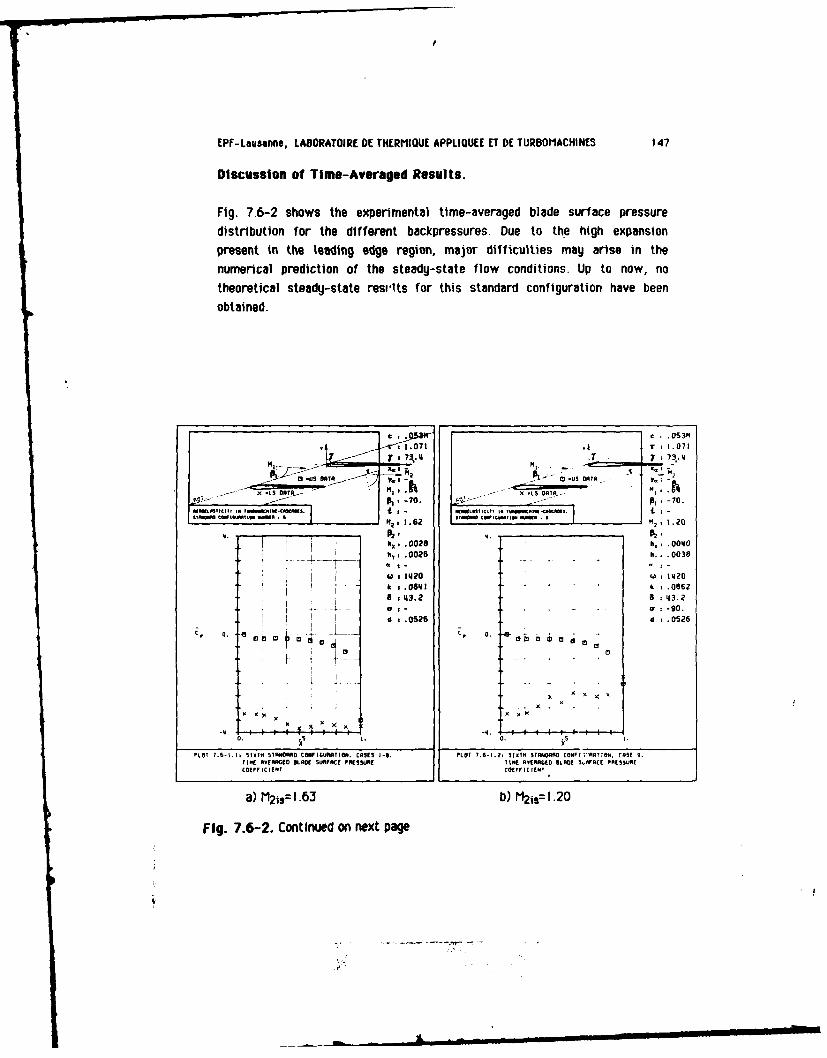
Efr-LaOMSan, LABORATOIRE DE THERMIQUE APPLIQUE CT DE TURBOMACHINES 147

Discussion of Time-Averaged Results.

Fig. 7.6-2 shows the experimental time-averaged blade surface pressuredistribution for the different backpressures. Due to the high expansionpresent in the leading edge region, major difficulties may arise in thenumerical prediction of the steady-state flow conditions. Up to now, notheoretical steady-state resilts for this standard configuration have beenobtained.

e, C .OS3MV-r.1.071 r 1.7

7 . 73.1 Y 7 7314&X.~ ~ ~ I 2 I N -

2 s 25 us ATA--.

p.-70. p1 -70.WRfLSIMhVT IN IANNKSJ-CICCS.Ia-.~I~~i 1 1 1~ m

K 2 .2,6 -M, 1.20

ft2 . .0028 bi, .0040by, .0026 h,1 .0038

W 1420 U1%120

k s.0641 -. - .0662843.2 a 1 43.2

aI 1 -90.~:.026 d.0526

0. a*-t, 0

a. M 5q 1.6 0.Mis .0I

Fig. 7.6-2. Continued on next page

AEROELASTICITY IN TURBOMACHINES: Standard Configurations 148

c,.053" A . . 05,W1.071 * -s 1.071

7 7.73.4 - 73..4

M, 'I- - -

Ha .1 ,P 1wc mJ, . , a 001 T IC-SSOA &9-U TA_

-~p-70. 0,.-70.

13 C s 1. 2 M~ 2.02PS, 4.P.

hm, .0040 b", .001h , .0038 _ T .0038

(., 1420 E ,1420k .0916 . ta.025

8 43.2 8 43.2Or - 92.... o" =-92.

d .0526 d : .0526

XXX U IC x

x U x x x

x

x

.. . . . . . t, .I0. .5I.U.SI

PLOT 7.6-1.3. SIXTH STANOARO CONFIGURATITN. CRS 10. PLOT 7.6-1.4, SIXTH STREOAR0 CONFIGURATION. CASE II.

TIME AfRAGES 0ARE0 SURFAC PRESI JE TIR E AVESRALE BLOME SURFACE PRESSURECOEFFICIENT COEFF IC IENT

c) M21 8=1.14 d) M2 3is=1.02

-r '1..071

_- 7 ; 7,I.

x T .- 70.

. ...... M, 2.00

k' Fig. 7.6-2. Time-averaged bladeg. [ ; [h 0, .0033

__,___ " .0031 surface pressure distribution for thew 10 aeroelastic test cases.! : __Ed a 2420

k a . 1039

8 :43.2

d .0526

xx x x x X< x

0. Is

PLOT 7.6-I.S, SIXTH ARUARO COM PIU ITA. CASE 1.

TIRE AVERRGEO SLRE SURFACE PRESSURECOEFFIC lENT

e) M21-.98

a.

EPF-Leusanne, LABORATOIRE DE TIIERMIQUE APPLIQUE ET DE TURBOMACHINES 149

Discussion of Time-Dependent Results.

At this time, as mentioned above, the aeroelastic forces have not been

determined experimentally. However, the experiments indicate regions of

self-started blade vibrations, i.e. domains where the aeroelastic forces arelarge enough to overcome the mechanical damping of the system. These

flutter limits are shown in Fig. 7.6-3, for three different aerodynamicexcitations. In the first, a well-tuned cascade (blade vibration frequency

f=230±0.5Hz) was used, with endplates at the tip of the blades to decreasethe aerodynamic excitation from tip-clearance flow. In the second, the same

cascade was tested, but without the endplates. Finally, in the third, thecascade was randomly mistuned (f=223,5Hz). It can be concluded that thO

mistuning, and the reduction of the secondary flow in the tip-clearance, damp

the blade vibrations.

t4 Strong vibration in 1. bending mode4V

34 (D Weii-tuned cascade with end-plates

2 Well-tuned cascade without end-plates28. - Mistuned cascade without end -plates

22-

16 --0.4 0.7 1.0 1.3 1.6M2.,

Fig. 7.6-3. Experimentally determined regions of self-started blade

vibrations (copied from /18/, Fig. 11).f 'f

AEROELASTICITY IN TURBOMACHINES: Standard Configurations 150

Theoretical results obtained from Method 10 indicate the same trend as the

experiments. This can be concluded from Fig. 7.6-4. Here, the blade vibration

is stable for subsonic, and unstable for supersonic, outlet flow conditions at

a -900 interblade phase angle (Fig. 7.6-4a; compare Fig. 7.6-3). At the

supersonic velocities the vibration is unstable for -180°<,<0O, whereas for

subsonic outlet flow conditions the vibration is stable for all Interblade

phase angles (Figs. 7.6-4b,c). The reasons for this instability are explained in

/18/ to come mainly from instability on the blade suction surface in the

throat region (Fig. 7.6-5).

COnCiuslm for the Sixth Standard ConfiguratiOn

The results of both the experiments and one prediction model(semi-actuator

disk theory, Method 10) indicate that the blade vibration in the sixth

configuration is unstable for supersonic outlet flow velocities in the

interblade phase angle range -l0°<o<O ° . The stability limits are accurately

determined by Method 1013

No comparisons between theoretical and experimental local blade surface

pressures could be made in the present study.

I

13 This is somewhat surprising as for the fourth standard configuration this

method showed large discrepancies between both the data and Method 7

(compare section 7.4). A possible explanation for this is the difference in

camber between the fourth (camber=450) and sixth (camber-140)configurations.

CPf-Lagsanne, LABORATOIRE DE THECMWEU APPLIQUCE ET DE TIJABOMAHINES 151

C .053-

7 1 73..

ONIiI M, x A

NiHA-70 -70~IW A N- 2

.

- Ii, .00216

u1%20 us1420It k t __ .0641

8 t t43.2

'A. zH -~' Sf43.2____

a\ I7 __04____

PLOT 7.5-6.5.,ESlOTM STANARD COIIGIJMTION. CASES 7.9-11.18. PLOT 7.6-6.I. SIOTA STANDARD CONFIGURATION. CASES 1-8.NEIONANIC WORK AD DAWMPIG COEFFICIENTS .,DOTMA"IC WORK AND DAMPING COEFFICIENTS

IN OEPENDA(CE OP OUTLET ISENSAOPIC VELOCITY 21 I I EPENANCE SF IATEANLASE PHASE ANGLE.

1)(1-900 b) 1i=1.63

1 '.1 .071

X -LS ATA K,

t:I0- Fig. 7.6-4. Theoretically determined-METHO0.98 asroelastic damping coefficient versus

-S.h,. .0020 iRefitropic outlet Mach number andfly .0026 tnteblad phase angle.' I-

(.61420- ft a 06%1

' 0. -I -4--

PLOT 7.6-.2. SIXTH STANWSm COW IGUMPTION.KEAOTXIC WAO AND OWMING CNEFFICIENTSIN AEPINOOACE OF INTINN.UI PHASE AE.

0) M 2*:0.98

AEROELASTICITY IN TURSOMACHINES: Stlndard Configurations I 5

9 .05341s c..own-S3" 1.071 4 1,071.T7; 73. 7 !:, 3.

. ...... ... .. T .. . .... . ... .- ' * 07

33 I3 1 4 8 '2: I .62 - ci'~ i 8 , 'Ii a , 1.•20

a x .0028 D I 20. .-0u0

-- b-- - - !.ih . 006 "-I .. ,, .00381. 4 .W ~z I 20 4 u:G1 2 "go G

z .008 .0062

S- _ 343.2 8 , ,e ,,3.2a -89. ","-90.

x .0526 2 [a: 026-ISO.~~0 LI-80 - 30

-10. ISO . 00.- -.- - -,, - .. ,o0. ---I, - -s~o.I I STABLE S TABLE

q* I0. -SO. L90. - i - -90.

S. 4 S) 0,US4 L S

1'

"g.-90"*. -20 . .90,

x x UNSTABLE' UNSTABLE"

-18. 18 -- 100. 4011 80--

ILOT "7.6-I2.?, 0XT1 0188080 CONFIGURATIN. Cas T. P.T 7.6-2.9, SIXT" STANDARD CONIFIEUATIOW. CASE 8.M0AIf 0 PME 436SE LEA0Of UNSIEROY BLAOE MA8,GN8ITUDE 80 P085! LEADI Of U817T6OT IADE50M't[ PRESSURE0 CIFFICIEN . SUROMI" PAESSUMSI COEFF C LB

a) M21=I.62 b) M21i81.2OC

1.071.7 3,.,

X 3 LS 00 OT

I- D.-70.

MI.-,----- .OW .a 1.13

SIX ,. -0040 Fig. 7.6-5. Time-dependent blade-- 1 - ST. .003 surface pressure coefficient.

Z', ,0. 1q20I0 .t .0916

•~ ~ 4 B 3.2

-92p -------- 6,- - -Z

d ,0526

0,(U~j# 0.

-Io. : . : ,0. -,

UNSTABLE"

PLOT 7.6-2.10' SIXT 5T808R8 Cow13208IS*,10, CASE 0.MGN0ITUD 880 P8838 LEO OF UNSTE8Or BLOSUIMRCI PF$SSUlI COFFICIENT.

c) Mlq= 1. 13

•,+ V:-

- i :., ";

EPF-Lausenne, LABORATOIRE DE THERMIQUE APPLIQUE ET DE TURBOMACHINES 153

7.7 Seventh Standard Configuration (Compressor Cascade inSupersonic Flow).

Definition

The seventh standard configuration has been tested in the detroit DieselAllison rectilinear air test facility, and the results are included here bycourtesy of the sponsoring agent, D.R. Boldman at NASA Lewis ResearchCenter (48, 491. The configuration is representative for the tip sections ofturboreactor fan stages (multiple circular arc transonic profiles. The profiles

are taken from the 86.7% span section of the second stage of the five-stageTF41-A 100 LP-IP compressor rig). Each blade (5 blades in the cascade) has a

chord of c=0.0762 m and a span of 0.0762 m, with a -1.300 net camber 3nd amaximum thickness-to-chord ratio of 0.034. The gap-to-chord ratio is 0.655and the stagger angle 61.550.The cascade geometry is given in Figure 7.7-1 and the profile coordinates in

Table 7.7-1.The airfoils oscillate in pitching mode round a pivot axis at (0.50, 0.00), witha frequency between 710 Hz and 730 Hz. The pitching amplitude of thereference blade lies between 0.06 ° and 0.2 ° , depending on the test conditions,with some scatter in the motion amplitudes between neighboring blades (dueto the high realistic frequencies).

Both the time-averaged and time-dependent instrumentation on this cascadeis extensive, and data have been obtained of different interblade phase anglesand axial velocity ratios. 20 blade surface pressure tappings were used (10 on

each surface) to determine the steady-state blade surface pressuredistribution and 12 dynamic pressure transducers were mounted on one blade(6 on each surface) to determinate the unsteady flow conditions.

Aeroelastic Test Cases

From the tests, a total of 12 aeroelastic test cases are presented here for

analyses.

These cases are included in Table 7.7-2, and they correspond to two different

time-averaged flow conditions. The inlet Mach number is the same in bothcases (M1 =1.315) and the outlet pressure ratio varies, corresponding to

M2 =1.25 and M2=0.99.The blade vibration frequencies of the tests are very high (f=725 Hz),

corresponding to reduced frequencies (based on semi-chord and inlet flow

I ~

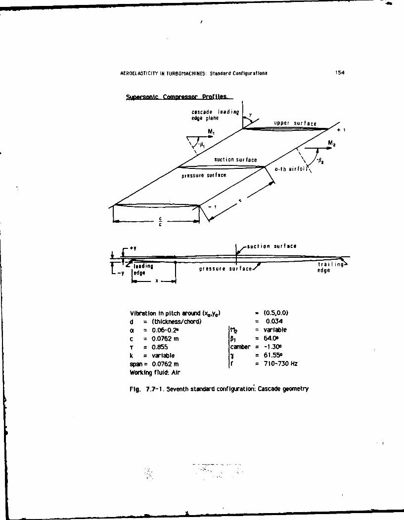
AEROELASTI CITY IN TURBOMACIIINES: Standard Configurations 154

%Xmm~oic CoMPr.Lo Prof iles-

kuto sufc v\ial T1 2 1.5

Woading fluid: Air

Fileg 7.-1revethstnd r coiurain e acd geoetr

EPF-Lausanne, LABORATOIRE DE THERMIQUE APPLIQUEE ElT DE TURBOMACHINES 155

C - 0.0762 0 (3.00 in)

Upper surface Lower surface

(SUCTIO SURFACE) , (PRESSURE SURFACE)

.Y X -Y

0 -0.0029 0 0.0029

0.0026 -0.0004 0.0027 0.0056

0.0278 0.0015 0.0279 0.0066

0.0655 0.0041 0.0657 0.0079

0.1032 0.0065 0.1035 0.0092

0.1410 0.0087 0.1412 0.0103

0.1788 0.0107 0.1790 0.0113

0.216S 0.01Z4 0.2168 0.0123

0.2S43 0.0139 0.ZS46 0.0131

0.2921 0.0132 0.2923 0.0138

0.3Z99 0.016Z 0.3301 0.0144

0.3551 0.0168 O.3SSZ 0.0148

0.3929 0.0175 0.3930 0.015Z

0.4307 0.0179 0.4308 0.0155

0.468S 0.0181 0.468S 0.0158

0.S063 0.0181 0.5063 0.01$9

0.5441 0.0179 0.5440 0.0159

O.S820 0.0174 0.5818 0.0158

0.6198 0.0167 0.619s 0.0156

0.6576 0.0158 0.6573 0.0153

0.6828 0.0150 0.6824 0.0131

0.720S 0.0137 0.7202 0.0146

0.7583 0.0122 0.7580 0.0140

0.7961 0.0105 0.7958 0.0133

0.8338 0.0087 0.8336 0.0124

0.8716 0.0067 0.6714 0.0112

0.9093 0.0047 0.9092 0.0098

0.9471 0.0026 0.9470 0.0082

0.9848 0.0003 0.9848 0.0063

0.9974 -0.000S 0.9974 0.0037

1.0000 -0.0029 1.0000 0.0029

L.E. RADIUS/C- 0.007

T.E. RADIUS/C- 0.0027

Table 7.7-1. Seventh standard configuration: Dimensionless airfoilcoordinates

AEROELASTICITY IN TURBOMA CHINES: Standard Configurations 156

4. - O

r-r L ,4 0 M I

+~ 0-r- % ur-ie a p r -

C1 -r %o~ r- D 4 0 PCr

-4 rled00 - -- C4 C4I N i

0 1000 00000i0 &

CNI 009000 666666,'D0 0

001000- 000000lD'~

0I 6o 0 0 -00000

W

R0 0 0m o0!0_ c 'D cn:)5 to %o01

tolo

CI t-~I + + + .ko In C % Oq

oZa - 0

CL 0-1 1 6 6 6C

C- . .

- cn

c,4Pn in w -c y

< ~ .j

EPF-Lausanne, LABORATOIRE DE THERMIQUE APPLIOUEE ET DE TURBOMACHINES 157

velocity) of approximately k=0.45. However, due to these high vibrationfrequencies, a certain amount of difficulty was encountered in the nominal

amplitudes and interblade phase angles, and in keeping these constant overthe five blades in the cascade [48, 491. Therefore, both the nominal and

measured amplitudes and interblade phase angles are given in Table 7.7-2. Asthe prediction models used for calculating the aeroelastic behavior of the

cascade consider travelling wave modes over a large number of blades it isexpected that some discreapancies between the experimental data and the

theoretical results will be present. Therefore, good agreement is hardly to beexpected. However, it should be noted that due to the considerablecomplications involved in measuring unsteady transonic flow in cascades, the

data presented are representative for the state-of-the-art of aeroelasticinvestigations on compressors in the transonic flow region.

Discussion of Time-Averaged Results

The 12 aeroelastic cases correspond, as mentioned above, to 2 steady-stateconditions (MI=1.315; M2 =1.25 and 0.99). The time-averaged data are given,

together with the results obtained from Methods 7 and 18, in Fig. 7.7-2. It is

seen that the trend of the predicted time-averaged blade surface pressurecoefficient agrees with the experimental data. However, absolute values donot agree well, either for the low (M2=1.25) or the high (M2=0.99) pressure

ratio case.For the lower pressure ratio, the Schlieren pictures indicate that the leading

edge shock is slightly detached and that it impinges on the blade suction

surface at about 90% chordwise position.

In the case of the higher pressure ratio, the Schlieren pictures indicateinstead a boundary layer separation downstream of the shock wave

intersection of the airfoil (at about 40% chord) [481. This separation wastaken into account in Method 7 by performing a boundary layer analyses and

then correcting the blade geometry to consider the increase in the

displacement thickness of the boundary layer [40]. The correct shock positionand exit flow conditions were obtained in Method 7' by adding this extra

thickness onto the aerofoil. However, no such attempt to match the

experimental data was made in Method 18, which to some extent may explainthe large differences between the two predicted results.

AEROELASTICITY IN TURBONIACIIINES: Standard Configurations 158

Discussion of Time-Dependent Results

When discussing the time-dependent results the experimentally determined

steady-state boundary layer separation at about 40% chord for the highpressure ratio should be kept in mind. Both prediction models 7 and 18 areinviscid and cannot deal with unsteady response to shock/boundary layerinteractions.

The non-constant blade vibration amplitudes and interblade phase angles inthe experiments also influence to a certain extent the agreement between thedata and the traveling wave analyses. It was shown in 1401 that a flat platetheory with variable blade vibration amplitudes agreed better with the datathan the same model assuming a constant blade vibration amplitude 140, 64].

c,.076m c .076MAj ".815 ,:.855

6t .55 ,_ _ _ " 7 :61.55

a -. T "Et,, M, M

M - U S D A T A . n ". .U D A AP Y 9

Va - r RE1VOD-

/ X -LS DATAr M , 1.315 • X -LS DATAR, 1. 1

OT D, -62.8 N P, -6.

WWI - i

-0.8 " " ".....r- EnO Ihx -6 . 0 . . -............... HE" TE HOO, P2 -6 .

ME - - - I0IHO 7 - - - - - -h, = - h,=

•" I (, = . "" .............. .. ................ ' (,J =

.. 8 : "x x . ° - : 8 -

. :.034 "d- .034

0, . ..........

i 4 10 . -

0. .5 I. 0. .5R x

PLOT 7,1-1.1* SEVENTH STANORO CONFIGURATION. CASES 1-5. PLOT 7.7-Il, SEVENTH STANDARD CONFIGURATION. CASES 7-12.TINE AVERAGED BLAOE SURFACE PRESSURE TIRE AVERAGE 8LROE SURFACE PRESSURE1STRIBUTION FOR OUTLET VELOCITT R?-IUS D ISTRIBUTION FOR OUTLET VELOCITy N 0 99 .

a) M2 = 1.25 b) M2 = 0.99

Fig. 7.7-2. Steady-state blade surface pressure distribution at Ml=1.315,p,=-64.0o.

EPF-Leusenne, LABORATOIRE DE THERMIQUE APPLIQUEE ET DE TURBOMACHINES 159

Intergrated values

The aeroelastic lift, moment and damping coefficients were calculated in the

experiments from the measured blade amplitude and the unsteady pressure

coefficient and its phase angle relative to the blade motion. The leading edge

and trailing edge values were obtained by extrapolating the 15% and 85%

chord data.For the low pressure ratio (M2=I .25, Fig. 7.7-3a) the trend of the aeroelastic

damping coefficient -3, versus the interblade phase angle, is correctly given bythe two models (7, 18) using the full blade geometry. This is also the case

for a flat plate analyses (Method 5), using a zero mean incidence angle (i.e.PI=-61.55°). All the theories predict the most stable situation around a=-

1200, and the most unstable around g=+450. This is also seen to be the casefor the data. However, the magnitude is different according to the different

theories.Also at the high pressure ratio (M2z=0.99, Fig. 7.7-3b), the trend of the

thoeries agrees well with the data. In the least stable position (w=+900) the

data and Method 18 indicate a slight instability, whereas Method 7 lies just

at the stability-line. It should be noted here that the stage was believed to

be deeply into flutter at M2=0.99 and out of flutter at M2=l .25 1401.

Considering the theoretical and experimental difficulties involved in

determining the unsteady flow in the transonic flow regime, and theexperimental accuracy (especially while integrating with 12 transducers at

the high pressure ratio), the results are encouraging.Also the calculation of the magnitude of the moment coefficient (Em) shows a

good agreement between the trend of the data and the theories, especially atthe low pressure ratio (Fig. 7.7-3c,d). However, a discrepancy can be found in

the phase angle. It is especially interesting to note that, although the

aerodynamic damping coefficient from Method 7 agrees well with the data atthe high pressure ratio (M2=1.25, Fig. 7.7-3b), a fairly large difference is

found in the moment coefficient (Fig. 7.7-3d). In the phase angle *m,

differences of up to A4m(=$m,Theoru - *m,Exp) =I80° are noted.The aeroelastic lift coefficient (El(t)) does not influence the stability of a

pure harmonic pitching motion. This information is given in Fig. 7.7-4 It isconcluded that the trend of the magnitude (El) is correct, but that the phase

angle (#I) shows a general discrepancy of up to =#jhl,Teory- l,Exp= 180 °

IL

AEROELASTICITY IN TURBOMIACHINES: Standard CArfigurations 160

.076M .076Hi, .855 • .855

IF 61.55 7161.55M .8 00 2 N -- *. N2M, M, K,, .5 MI .,s

y0 0 . y. 10.

, D.TPi 1.31S X .5 OI Mn, 1.315I -64.0 p1 ,-64.0

MOL~I ll I l18DATAWE. C- cs l -~ I 1. I.11 -DATsL i CII .. . ..... .. 2 1.25 M2,

0.99.. .. . 8(T1 0 1 ... .. . 18t00 7.2 . . , p -62 .8 -2 - . p , 6 3 .6

. . .00; tO n, - iM D -

Ill - ih -

-s.4 .. ik a .44C8- 8 ,-

d .034 d .034

0.! - INS TABLE C UNST. -I .

r .TABLE I - STABLE

,180. 0 Io. -80. 0. 100.a or

PLOT 7.7-6.1, 5(08Y78 STONDOOD 0 CONFICURATION. CS 5 0.6 PL t 7.7.6.2, SEVE O STANDAtR DO COW:GOURATION, CR5 71 12.R0R800T [IC C 0;; All OOPI G CTEfP If {,.l5 O[ooriAoff CORK A. 0 ~ DIMlG COEFFICIt' 51N 0(P80fN OF . I 0' 8I.0 ( ,EL CN OEP, O CC 0' ICT(RB100( PCAS[ 1 C-LI.

a) Damping coefficient, I1 : 1.25 b) Damping coefficient, Mz= 0.99

c .076 076"

r.855 As85, a 6 1 .5 5 -" , 6 1 . 5 5

PIT • x .5 .S.(n U S AT A MI35 .x. y:O

V.t 0. (n us Data 00Y. a 0.-1. DATA M, 1.315

640, -65 DATA -64.0

M, , I.25 z ,. 99

2. - - po-62.8 2. • - - -- O- o 2 -63.6

- -s,,is, -.-

is .0)q to ".4

I . ! ] .0.0

I O, 5 1,Ito. .

AI. so. . too

C)g Moment Aoff cernaM c12 d )min Momen-t crof f ic int, M2ers0us

interlade phase angle for Mz = 125 a M2 = 0 99

. l Jl n81i'm i i 0 ml l i SO

161

Blade Surface Pressure Differences

The trend of the magnitude of the time-dependent blade surface pressurediference coefficient (&AY is correctily predicted at the low pressure ratio(M2=1.25, Fig. 7.7-5). However, the predicted phase angles disagree with themeasured ones, along the whole chord, while the theories agree well witheach other.The flat plate analyses (Method 5) predicts a discontinuity in a at theposition where the trailing edge shock impinges on the blade pressure surface(xshock=0.55).

N1 .. S

~.s~y p -6'4.0 IL 66.0

1,. '0 .

-034

U.,-

a - - -S. aadI77,2N 7>I V. l," MW I P.--

a) Lift coefficient, P1 = 1.25 b) Lift c@fvi Iien~t, Piz= 0.99

Fig. 7.7-4. Arov'nwic lift coefficient versa interblade ~hi angleforPI2= I 25 andNM= 0"9

AEROCLATICITY IN TURBOM"AMME& 3. tandord ConfiguriltIons 162

c c -6 .06

Y. .0 a-u at . .

u14 .0 0 6'I

N I . I N 20 1 .2.s1 -

-______ _ 8 .099.0142

a 1 -1 0 9

0.

-90.-

too. f. 1. wv 6 s-4in 1n. -180. 41~ I-

0. 0. S0

c 076"n. .0760

a* usC, -SDT . 0

-64.0 -62.0OhAi, .swwf - got - ,

__________I A< 4 .. -low,4

0 * 0

0"

ts, af I

Wad Moosec prrdl? cafc1

c) a = 0d az+Fig 7 7-5. o-ewo iieWc roi i ~V#COfIW

laNg btae chwua N t12

EPF-Lausenne, LADORATOIRE DE TNCRMIQUE APPLIQUEE CLT DE TURBOMACINES 163

Some slight indication of this can possibly also be found in the experimentaldata, whereas Method 7 smears out the unsteady response of the shockimpingement on the blade. Away from this region, the flat plate analyses

(Method 5) and the full geometry, potential flow solver (Method 7) givesimilar results.Also at the higher pressure ratio the trend of the magnitude (.Zp) as

predicted by the theories agrees well with the data, both for the flat plateand full geometry solvers. Again, the phase angle (#a,) is not well predicted.

.076 .. 076Mss .855 jT .855

7 :61.55 - T 61.55

X LS AM, 1.315 M0, 1.315I -64.0 P,, -64.0

I m * A CW9 IS... ... . . .a i9 M2 99

20. _; & .-6. 20.- - - -A. 00 7 A2-63.6

m I D 7 h,,-- A-- -,- - - - i - A,

- .1020 11S7

ae, W -1- 555 a1, 6. 044 A 44

as

dd . d I .031

0. .+..44..44...

-IS O.',A . ___U0.

UNSTABLE- NSA' BLE

0,, o. . 1 "-, o. H L _ _ _ __9"

9 . 90.ST-10(

AK E I-. II"

- 0'..

P1.O? 7'.7-$1A SAC AYM $TAlOAm CNIOGuSStf. M A. PLOT 7.7 3.9, SIV TO STAIA CO IGOTION. Case 9MUAITADE me0 P160 LEA IO F U LAO SURFACE AAGA1I TI4I ANI POAME LEAD OP BLADE STO,Pl1191 OFFI PI C COEFFICIIT. PAWSSUOAE OIFFIEC(E COEFFICIN(

a) o=-450 b) a = 00

Fig. 7.7-6. Time-dependent blade surface pressure difference coefficientalong blade chord at M2 = 0.99.

AEROELA3TICITY IN TURDOMACtIINCS: 5tandard Confhiuratlon$ 164

Blade Surface Pressures

From the few predicted blade surface pressure results obtained on thiscascade, a modest agreement is found in the magnitude (EpU3, Ep1) both for

M2=1.25 and M2=0.99. Again, discrepancies are found in the phase angles (Fig.

7.7-7), especially towards the trailing edge region where the experimentsindicate a boundary layer separation. However, these differences seem to besmaller than the corresponding ones for the pressure difference (46,).

Conclusions for the Seventh Standard Configuration

From the study on a 3% thick, low cambered compressor profile in supersonicflow at a high reduced frequency, oscillating in pitching mode, it can beconcluded that:* The experimental steady-state blade surface pressure distributioncannot be fully reproduced by theoretical methods. Indications of the boundarylayer separations on the suction surface on the aft part of the blade exist.This phenomenon certainly influences both the steady-state and time-dependent flow response., The experimental blade vibration amplitudes and interblade phaseangles were not constant between the 5 blades in the cascade (Table 7.7-2).This fact influences the agreement with the traveling wave analyses. It isexpected that the agreement would be better if the prediction models alsoconsidered non-constant blade vibration amplitudes and interblade phase

angles.

0 Both the experiment and the available theories indicate the same trendsfor the aeroelastic damping coefficient versus the interblade phase angle andoutlet flow velocity. The magnitude Is however not fully predictable.* The range of predicted instabilities, or near instabilities, agrees wellwith the experimenta data.

0 For low pressure ratios the stability margins are predicted just as wellwith a flat plate anlyses as with models considering the full blade geometry.0 The amplitudes of Zm(t), 0(x,t) and ZlUS,l8(x,t) are modestly well

predicted. However, the corresponding phase angles do not agree with ther data. Again, for low pressure ratios, the flat plate analyses agree well with

the full geometry solvers.0 Further work, both experimental and theoretical, is necessary toestablish the origin of the differences found in this standard configuration.

.. . 7.' -

rP' -Lau6enne, LABORATOIRE DE THCRMIQUE APPLIQUEC T DE TURBOIACIINCS 165

.075H- ~ c .076M- a.ss r.855/ :61.55 .' :61.55

MI. 6 s -, x. .5

C) -US DATA . Y 1 .0 PIT m -US ORTA P2 V 1 .k M, , 1.3151 5- DS ATA IPT 1.315

p.,-6A.A0 - p1, -64.0

ULyMTICm IotSmt IISC4IS ,ASCS2 -•2 AS TIErlt It mva TIB mHI 14, UM - '

I',to . . ............... .... M OR, -Tp ,-52.0 10. -- me--, o 9.0 S,-62.8

j .0699 .205 s e, S. 119555

d .031 If ..034

0 . I '- -1 , ; , I

x. .•A ..... .

(S . - I(LI IUI ( I5

-90. 90, -90.0

13 t

MAGNMITUDE AN0 FAASE LEAD OF BLADE SURFACE MAGAITU0D ABA PlATJE LEA0 OF BLADE SIIBFACE

PBES5URE COEFFICIENT. PBB55UAE CBEFFICIEAeT.

a)Mr 2= 1.25, O = 10OO )M 2 =- 1.25. 0 --4C3 € .076 |, c0076

7 Tr . 055 .- T .055

•-. 7: s61.55 '-' 61.55I - I~A . A1 . - .15

I2c u m .- a"-- 1P 9D. 0 P1 I .0 DATA . 0

A , 1 . -L5 D A - 18 .10

- I0 . 2 5 0. 9 9

a) M2, 1 .25 (1--0b 2 .5 -5

T As Ass

T .217? . .1020

k .fu:54 I u,14555

4. At 61. 6 1

PI ... us o t 0 PI M -u-DTA.

X LSA LS, AIR0• I - IT ,.

c_ _ . LW ' sTAI * INNAI '', N,

. ... .. -5 2 . 20 A W I3 .I

a t

As5, a- 4

N o So 0k

0 ) 4' 1 , 1 1 01 d) 4- .0 110.= 4

S . .........to I LI I i

I rt, 1 if It WU. SiBACAB (fnIIA I sit 4. IsI 1 B. ifffB.' TBBC . IWK ITUOI AND -. 011 14 c O D IOB f I( !I' SAC0( mw USA Inv &I" I FAP 004ftBswof (allf lIt,Sl.A A~~

0 cM 2 = 1.25a00 d) pi 0-9Q, a=-459Fig. 7.7-7. Time-dependen bladb mlIe Presie coetficlent a10gblad hod atP 1 .125 eNW 1 2 0.99.

AIROELASTICITY IN TIJRSOMACIIINES: Standard Conl'lqurstlon3 166

Pt-Lausanfle, LABORATOIRE DE TM[RrIIQUC APPLIQU[[ ET DE TUROOt'ACMIN[3 107

7.8 Eighth Standard Configuration (Flat Plate Cascade in Subsonicand Supersonic Flow)

Definition

The eighth and ninth standard configurations are directed towards theinvestigation of basic aeroelastic phenomena and the influence of thickness

effects on numerical calculations, especially In the transonic flow region.

Configuration number eight deals with a two-dimensional cascade of flatplates. Theoretical analyses of such unsteady configurations have beenperformed for many years now, but the problem is still of great interest,mainly due to the following factors:0 In modern compressors, operating in the transonic and supersonic flowregimes, the actual blades are rather thin and have a low camber. They can

thus mostly be fairly well approximated as flat plates0 Supersonic two-dimensional flat plate prediction models are often oneof the main aeroelestic tools used by the designer of large turboreactors0 In the incompressible flow domain, analytical flat plate solutions areavailable.* It is possible to establish, with different theories and for the purposesof the present comparative work, the aeroelastic response of a flat platecascade over the whole Mach number range from incompressible to supersonic

floIw conditions.0 The strip theory assumption should be validated, in the transonic flow

domain, in a fairly simple case This requires validation not only oftheoretical results, but also of two-dimensional and quasi three-dimensionalexperimental data on thin airfoils

The cascade being Investigated as the eight standard configuration Is shownin Fig 7 0-I

Aerelestic Test Cass

In this eight standard configuration, the main emphasis will be laid on thechange in the aeroelastic behavior of the cascade in dependence of the inletflow velocity, pressure ratio through the cascade, stagger angle and solidityThe U"steadyj blade surface pressure distributions will thus be compared Indetail only for a few aroelastic casesIt Is assumed that the two-dimefsional airfoils oscillate in pitch about mid-chord (0 5, 0), with an amplitude of 2" (0 0349 red)

• I

AEROCLAOTICITY IN TURDOrIACNINE: otenuaro conrigurations IO0

As the main interest for this configuration lies in the variation of the time-

averaged parameters the calculations should be performed at zero meanincidence, with a constant interblade phase angle of 900 and with a fairlyhigh reduced frequency, k= 1.0.

During the project it was found that this high reduced frequency mayintroduce inaccuracies in the calculated results. However, such problems areof special interest in workshops of the present kind, so the results arepresented nonetheless.

35 aeroelastic test cases have been selected for analyses (Table 7.8-1). Thisis the largest number of test cases for any single standard configuration,which may seem strange for such a simple configuaration. However, as can beseen from Table 6.1, a larger number of predictions were made using thisstandard configuration than any other. This is clearly the case as more flatplate prediction models exist than methods which take into account the fullgeometry of the profiles.

Flat Plate Profilemecascade leading

edge plane

LY pper surface /

.4

Vibration In pitch round (xy 5) = (0.5,0.)

a - 2.00 (u0.0349 rid)c a 0.1 m II = 00r - vrill.(0.5-1.0) Icw.er 00

kt = 1.0 ji =vaiale (00Sa 90* variable (0.0-1.5)

Fi. 7.5-1. Etth dwds coniguawtwn: Cascade geometry

_ i I l l I l l I I'I mIII I I • I I m i e .

•.

EPr- Lausanne, LAVORATOIRE Or TflCRM1QUC AFPLIOUCC CT Or TURBOflACflIRC

Time - Averaged

L) zZ1 Normal Shock

(0) (0

1 Incompressible 0 60 0 752 4

3 304 IF10

5 0.5 606 067 03 7a 0.69 0910 0.95

I I 0Z8 4512 3013 014 c0 0.5

15 ___ --- L.16 1.1 07517 4at L.E.18 ______ at L.E19 1.220 4at I.E.21 ______ at I.E.22 1.323 4at L.E.24 _______at I-.E.25 1.426 4at I.E,27 _______at L.E.28 1.529 4at I.E.30 ________ at I.E. ___

31 130.532 1 0

33 at LE 0.534 41.035 _____45 075

Table 7.0- 1 Eighth Standard Configuration 35 recommendedaeroelastic test cases

AEROELASTICITY IN TURIB0MAC"INE3: St~afld Coariguratorns 170

Discussion of Time-Dependent Results

In total eight models were used to predict the unsteady flow around the flatplate cascade. In general, the results of the different analyses agree well,with a few notable exceptions.

Integrated parameters

The first results presented are taken from the investigation regarding theinfluence of the steady-state stagger angle on the aerodyjnamic dampingcoefficient (Fig. 7.8-2).It is found that the results obtained from the different prediction modelsagree extremly well for a low subsonic flow velocity (Fig. 7.8.-2a),whereas some

c0. 1 0 I0s.7S C .0.751

0 ~ ~ 2 )-US ORt 7.M A 0.0500 o o~ .I~o -U . )TO.

A X LS ATA X~O X.LS OA M,0.8

_ 400 0IT4 Wan 2hMTOO M . M2 -8

- : 0349- s:0349

- hs.0 11.0

a 90. 9 0.4

0. C. TAL S 0. ___________ ~ uNTA0ISTABLE SAL

: : : 1I DO 0.: S100,

PLO 16.1, EIGHT" STANOWB COW IGI"MA I 101 C Asts 1-4. PLO' .- 12 £ 10 1 ANW060 CONFIGURATION. CASES B. I -13UafOOOYIONIC MORM am ~!N&, COEFFICIETS AFAoeosNsC meow AND DAMPING COMPICI ENT

L0 PLOT 7- 1. E I0O STAGCT. 0000£ 1. U(PfNOMHC1 Of S01061 ANGLE,

a) l1,=O. ) M1=O.8Fig. 7.8-2. Aerodynamic damping coefficient versus stagger angle for

M,=O. and M,=0.8. respectively.

CPr-LOUsenne, LAVORATOIRC DE TIRrlIQU APPLIQUEC Cr DE TUROOP1ACs1NE 171

discrepancies appear at a high subsonic flow velocity (M1=0.6, Fig. 7.8-2b).However, all the methods predict stability for subsonic Mach numbers at thespecified time-dependent flow conditions (k= 1.0, ir=90°).The good agreement between the theories, for subsonic flow, is also seen inthe aerodynamic damping coefficient versus Mach number (Fig. 7.6-3a).Here, the differences in "a between Ml=0.0 and MI=0.5 come about because ofthe interpolation-routine in the plot program, and the sharp.peak at M1=0.5depends on the closeness to the acoustic resonance (M1 ,ac.res=0. 53 ). However,some small differences can be found between the different analyses at thehigher flow velocities (MI>0.5). These differences become somewhat larger

for supersonic flow conditions.If a strong shock is positioned at the leading or trailing edge (Figs. 7.6-3b,c,respectively) the potential flow solver 7 predicts only a slight change inmagnitude of the aerodynamic damping. However, a flat plate anlyses (Method19), with special care taken in simulating the leading edge shock (Fig. 7.8-3b), predicts instead an instability in the Mach number range .3<MI<1.5. Thereasons for these differences are not apparent at the present time, but it isfound (Fig. 7.8-3d) that differences between Methods 7 and 19 exist in boththe magnitude and phase angle of the moment coefficient (Em and #m, resp.).

Blade surface oressure differences

At low subsonic flow velocities the results obtained from the differentprediction models agree extremly well (Fig. 7.8-4a, where 1=60 ° , lt=0.75).This is also seen to be the case at higher flow velocities (Fig. 7.8-4b,M,=0.8). Evaluating these results, it can be seen that the differences inaerodynamic damping coefficient at MI=0.8 (Fig,7.8-3a) probably come aboutbecause of a slight discrepancy in the magnitude of the blade surfacepressure difference (W) In the different models.However, the trend is the same for all models, both as regards the magnitude(A) and phase angle (06,).For supersonic flow velocities a larger disagreement is found in the pressuredifference coefficient (Fig. 7.8-5). The trend of AE, is the same for two flatplate analyses (Methods 5 and 19 in Fig. 7.8-5a), whereas a finite elementpotential flow solver (Method 7 ) does not indicate any specific

AEROELA3TICITY IN TURCOMACMINC!: 3tandar0 Conrlguration3 I 72

C 0.. I . 0.T :0.75 T 0.757 60. " - . 7 60.

, - , n2 l 0.5 M, .- 0.5

0 US A5 -t 0 - ns B IA ."

0. P1~ I .. . .11 0212 p2x' -' -LS O T I' - LS -D o,-60. b. -60.

bf~I~lIN,,C~ 1Cn.0. 1 AIC~b U1 C m 0.

... . . .. . . IE1h10 7 ll lb .

-- OO - - 1OO 7-R. WD 1.k-Nf2E 7 0 h 2 , -I

T

.0349 .0349

. ,O1.0 b 1.06:- 6I-

a 90. " 90.A It : % :STO I I d -

0 . U N 7A B L E 0 : "

A1 5,1O

Ilo CfP(O66F OF 626' 6606 MAMA ;NO S6( I3O7CN I N..6..( 66 2116,w.'

a) No strong shock b) Strong leading edge shockN O. IN 1 0 .1

.1 10.7S " 07S-I-. 60. _ .60

, . 0. -S

0 OV5 D'. 0..15 D6TA

P, 60. jso0l 1 0

d 6

A- "Af I

* 03%9 .-

A,

IIAiAI cmA,

c) Strong trailing Op s d) Strong leadi~ng edgeF i . 7.8-3. Aerodyna ic lmpng and monwt coefficients vrt-

I z HI•. -mil Ni i ii

l

.... _ _u

6111 66 I ~ 'N~fl - c,~ -e -A

173

*:hange, either in At or in #&p, in the neighborhood of the steady state (weak)

shock wave impingement on the blade surfaces (see sketches in Figs. 7.8-5;

xShock=O 62 on the lower surface, xShock=0. 9 5 on the upper surface). However,

the flat plate analyses also show some disagreement in the case of a detailed

companson

If a strong shock wave is positioned at the leading edge (Fig. 7.8-5b), the

finite element solver (Method 7) indicates some change along the whole chord,

both for the magnitude and phase angle (,&Ep, #A,). Here, the differences

between the two methods are larger than in the case with weak shocks. The

discrepancy is fairly large for both the magnitude and the phase angle. From

this Figure. it is clear why the stability of the cascade was different in

Methods 7 and 19 (Fig 78-3b) In the forward part of the blade the phase

angle #,p indicates instability for both methods. However, for Method 7 this

phase angle is close to

c , 0. IMr 0.75 " - : 0.75

-, 0.5 ____III .- H2. 0.

, .0. -15 AT M , 0.8

i.Il 60. . ,-60.M2 --

-, .034iE .. OD. 2 hxmf- " ... ME TRW I S'

.039 - -- - --- 0 ; .0349

1 .0 k 1.0

+- ... ..-a 90, O 90.d d -

+o

" f USTABLE

0 I' S'1111R CN ICUA1 AES

OL-AC 1 UD 4D,'S LEA OF 80TED B'0LAD

SUW QC '80VE IFAKEDSRIU1* 90

a) =0 b) MI:0.8

Fig . 7 81-4- Blade surface pressure difference coefficient for

differmt subsonic flow velocities.

* .8II I I I I I I II I l III

AEROELA3TICITY IN TURBOMACMINE. 3tenaard Conliquratlons 74

C 0.1,.1 6 0.I.

r 0. 75: 60.

16sK. l I 5

Pt -us 0Aa ,

I I PIT

C_ _ _ 0r: g . V. • 0

Xt -L DATA _W

60106160,0. 0..

-- -... - , 7 /'

.. -..... . . .-

-90.. . .90. 9.

-I, ;i A - - - ./ A .

1 0. 0. L

PLOT 7.8-3.22, EIGHTH STAN ORR CONFIGURATION. CA E 22. PLOT 7.9-3.a3, EIG T ST .0 O COW[P AT, 0%. -50 2MAGNITUDE AND PHASE LE D OF UNSTEADY BLADE 000 1GN TU 0 AND _665( (60 V6 ,, C ,

,VSURFACE PRE55URE DIFFERENCE DISTRIBUTION. SURFACE PRESSURE 010,0E66.(6 1 ' 8,F 0.

a) No strong shock b) Strong leading edge shock

C . 0.1111 0.75:60.

P1 0.5 DT1.1066R MY .1.3,- s "6 "t"P IT -60.

MMSTI ICoIrIUTTIOC '16 6t.C0S16. I ONI .0616

SO-- 7 P2S

: 034 9

o 90.I. , :i o -- d ,

: I IUNSTABLE'90. I

0.

-90.

'00$TBLE

1.8" +. 3. 4J E I HTH 51ANCARD CONFIGURATION, CASE 24.MAC NITU0E AND PHASE LEAD OF UNSTEADY BLADOE+ UR4F+(E PRtS tjAE OtIFEREfNCE OtIRI UTION.

0) Strong trailing edge shockFig. 7.8-5. Wade surface pressure difference coefficient for

different shock positions.

0.l

M-.LeOfm, LAGWAVIN~ K TigCtegs *Pft19t It IN TuRSOfaMugOW

fr hoe for Meto~td 19 it is close to .9(r Theref ore, the forward part ofthe iod dea not cotriute o 0 large extent to the loredtiil domuing

for Method 7. whereas it dos for Method 19 For both methods. the leedmnqedge shockwave .s c oInVa sena an increase in n1I Ude (xgm* zO 65. ig7 8-5b), althouh to a similar extent for the potentiul flow solver then forthe analytical flat plate medel In the latter, the shock woke is alsonoticooble as a jwim in the ~ha angle, wherma the former does not showlb UN~ signif icant ifluenceIn Fig 7 6-S5c the sam calculation is presened, but with a strong trailingedge shock wove insead of a loading edge one Woe, results ors available forthe potential flow solver only The ini IVmnm of the shockweve on the blesurfaces is noted (m, =0 35), both in megntuf and ~hs It is interesingto note that, although the aereqpiemic domiing coefficient did not chanlgesignificantly (according to l ohod 7) if the steady-state shock wove waspositioned at the lading or trailing edge (Fig 7 6- 36,c), the blae unlacPressure difference coefficient change along the whole chord. in a non-negligible maniner, for both the magnitude and phase angle (Fig 7 8-5b,c, notehowever the difference in scale in At.)

Sledo surfacea rasures

As for £A9(x, t0, the local surac pressurs (U."(xO), 1010(o) uextremely well in two different potential flow methods for s4sNwic Machnumbers (Fig. 7 8-6), both as regards the magitude and phase angleFor supersonic velo1citisS, only two resuts (Methods 7 and 9) were submit ted(for all results, see Appendix A5)The potential flow solver (Method 7) gives almost identical resuts for thecase with weak shocks (Fig 7 5-7a) and with a strong trailing edge shock(Fig 7 8-7c), apart from the lower surface in the vicinity of the strong shockwave (xsw&kO 35).However, for a leading edge shock wave the rsponse is quite different (Fig7 8-7b) Here, as already found for h~p(x,t), there are some larg differencesbetween the Methods 7 and 19 Presently, no explanation for this can be given

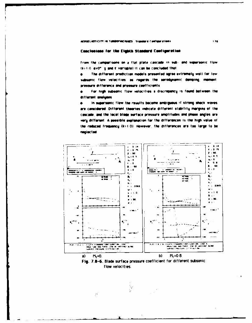
Cmbemkm tar lle FW Stlm Iu Ceoflgm'ette

From the con"wrigrng on a flat 0late Cscaf inl sta- and ,sontwc flow

(k= 1 0 OW0 1 and V aflel) it can be concluded that

41 The different Proilict ian models prosened a"e extremIV~ well for low

14hs1c flow velocities a" rgWas Ite Sadynam"IC danig. menent

pressure differenc and Preesure coefficients0 For high susonic flow velocities a discreanclI is found bewee the

Ottfoes "ntyes

0 in "MseruWC flow the revlts Deco"e aniguous of strUwg shock waves

We C01111111111 Dhifernt theories indicate different stablity rgins of the

cascade. aw4 the local blae surfce pressure amiitudes and pliese angles are

verjV differen A amosible e"Ieaneon for the difference.; is the MIAi value of

the reduced fresiencti (kz 0) However, the differences we too large to be

neglected

r* 0 U * ?.0

- . 0 S 0~ 0

.0 05

0. OsC

*~~ 90. 9 ~* - .1 0.

1 , fw

a, It cow

IN .0)9 -- 5 .00W)Sto

a) 1,=O b) M=.

flolveociies

EFF-LOUSeUfte, LAGORATOIRE D1 T~utrlg APPLIQUEE rT DE TURBOMACIIINE3 177

4 . 0 In C 0.104

v30.7S 7 10.7s

41 1. 7.6S0.- ; " - A. 1 0.51 -o.0.

WAMMI 0"-8*~888 p1 -60.

1 . 0 . 0 18 , 8b .

.0349 .03119

030STBL '90 .U,- I

0 .0 I

~80 . 0 - .10. j.80.

- - . 310 *80.f 40

0 x - *

j. 0.7

P, . 0.1.0

k .0

0.760

0.8.0.

is (

PLO .-. 2,EG7 ~ . S8I8 COFIURTIN CAE . 3.i3 1u~ no0438EOOFUSEAYOA

difeen shc poiiosatM=13

ACROCLA3TIC ITT IN TUROIIACflINC: 5tgfldard Co M19urtOAS 178

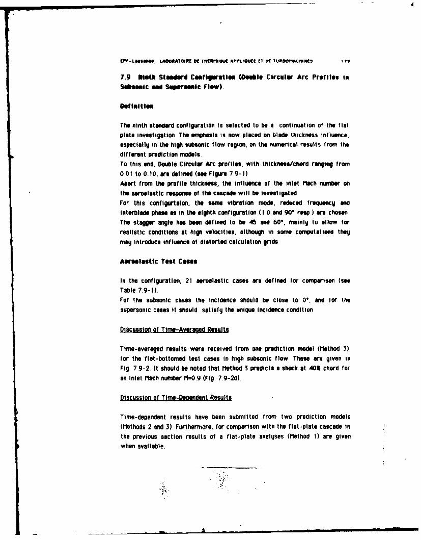
U

CP-LeoU$en, LAOOIATWORt TntRrIrNC lt AIPPLIOUCE CT PC TUROOMACtmNm

7.9 Ninth Standard Cefiguratie (Double Circular Arc Profiles in

Subsonic and Supersonic Flow).

Definition

The ninth standard configuration is selected to be a continuation of the flatplate investigation The emphasis is now placed on blade thickness influence.especially in the high subsonic flow region, on the numerical results from thedifferent prediction modelsTo this end, Double Circular Arc profiles, with thickness/chord ranging from

001 to 0.10, are defined (see Figure 79-I)

Apart from the profile thickness, the influence of the inlet Mach nwmber on

the aeroelastic response of the cascade will be investigatedFor this configurtaion, the same vibration mode, reduced freiquency end

interblade phase as in the eighth configuration (I 0 and 90 reasp ) are chosenThe stagger angle has been defined to be 45 and 60", mainly to allow for

realistic conditions at high velocities, although in some computations theymay introduce influence of distorted calculation grids

Aeruelastic Test Cases

In the configuration, 21 aeroelastic cases are defined for comparison (seeTable 7.9- I).For the subsonic cases the incidence should be close to 0", and for the

supersonic cases It should satisfy the unique incidence condition

Discussion of Time-Averaoed Results

Time-averaged results were received from one prediction model (Method 3),

for the flat-bottomed test cases in high subsonic flow These are given inFig. 7.9-2. It should be noted that Method 3 predicts a shock at 40X chord for

an inlet Mach number 11=0.9 (Fig. 7.9-2d)

Discussion of Time-Deendent Results

Time-dependent results have been submitted from two prediction models(Methods 2 and 3). Furthermore, for comparison with the flat-plate cascade inthe previous section results of a flat-plate analyses (Method 1) are givenwhen available.

PAMILAWtgCIT I gTURSOnACOmats 5mWo cowpr.iwas ISO

~flei~h -~t~ La ..........1

Ye() muHEI,.-R.(R*2-(X-0.5)?@S It H6003 0 if H2.0

gp~i t I ifor Fb/0O* 3 ~upu. varfme- * 10w rt WWI

Miximum thicknss at x = 0.5VmrgtInin pitch vmj (xa.yo) = (0.5.camn-Ilt)d - (thkdmshmdwd) a 0.01 -0.1a z 2.00 (m3.0349 rid) I#wc a 0.1im 11 00(for M fl.)T z 0.75 Icmnbor 00 (forsymmetric ProtIa)k - 1.0 45, 0ps - vamobe (0.0- 1.5)

Fig. 7.9- 1. Ninth staird conf Igiraton: Cascads bometry

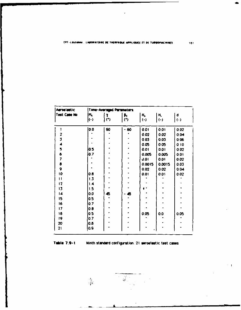
WP-LUS0 , LOMATO K TItUsOt APPULOUC fT Pt TU*JOflACWIMWU

AMlMtlc TIuw-AMVerg PuWWetS__ __-___ ___ _ I () _ _ _ h ) I-) I -)

1 0.0 60 -60 0.01 0.01 0022 0.02 0.02 0.043 " 0.03 0.03 0.064 0.05 0.05 0105 0.5 0.01 0.01 0.026 0.7 0.005 0.005 0.017 0.01 0.01 0.02

"a0.0015 0.0015 0.039 0.02 0.02 0.0410 0.6 " 0.01 0.01 0.0211 1.3 " "I? 1.413 1.5 -14 0.0 45 -4515 0.516 0.717 0.81 a 0.5 0.05 0.0 0.0519 0.7 " -

20 0.821 0.9

Table 7.9-I Ninth stdard configuration. 21 seroelastic test cases

VI.

AfROELA3TILTY IN TUR8OtACfINCD 3andalrd Confiquratiofihs 82

Integr attd Pat ameter

The trend and magnitude of the aerodynamic damping coefficient of the

,lifferent models versus inlet Mach number agree well for a 2 thick

symmetrir double circular arc profile (Fig 79-3a)14 in the high subsonic

flow region the flat plate analyses predicts a somewhat higher aerodynamic

damping than the potential flow models Or a flat-bottomed. 5% thick, profile

some larger differences are found (Fig 7 9-3b)

Blade Surface Pressure Differences

The unsteady blade surface pressure difference distribution was submitted

for several aeroelastic test cases For moderate thicknesses, symmetric

blades, and low Mach numbers (MzO 0) the full geometry models predict thesame unsteady behavior as the flat-plate analyses (Fig 7 9-4a) For 10X

thickness, a slight difference is found (Fig 7 9-4b)At higher Mach numbers, differences are found at lower thicknesses (Fig 7 9-

5)

For the supersonic inlet flow conditions, only one prediction mode) was

submitted (Fig 7 9-b) This model indicates the same pressure response forI 3<M1<l 5, with a 2% thick airfoil This is clearly the case as, for Mach

numbers larger than MI:I 3, the leading edge shock wave passes downstream

of the trailing edge of the neighboring blade (compare Fig 7 8-5a) The

results obtained from a 5X thick flat-bottomed DCA-cascade, at high subsonicinlet flow conditions, show larger differences between the flat-plate

analyses (Method I) and a potential flow solver (hethod 3) than on the

symmetric profiles These results are given in Fig 7 9-7As the Mach numtbr increases from Mi=0 5 (Fig 7 9-7a) to M,:0 9 (Fig 7 9-

7d), it is found that the differences between the flat plate analyses and thepotential flow theory increase, both in magnitude (-p) and phase angle (46p)For the highest Mach number the Influence of the shock (at xshock=0.4) Is

clearly seen with the potential flow solver (method 3), whereas the flat plate

anlyses indicates different distributions for AE and' 4Ap (Fig 7.9-7d).

CPF-LO44s11811, LABORATOIM! VE TIIRM APPLIQUE[ CT VC TUROflACMINCO 0

-. 80.10 C 0. 1"

a -US0.5 K1 -U Dal. 0.

0.1 K1 .0.1

4 -. me Kp

* .. 0369 .03,19

W I- W8,-

I * 9,2~.0 &..

........ 0,90

1 0.

PLOT 1.9 1 1 0 T 3410110 CWI&4?IU. can Ill. PLO, 1. . 1 ? IW. 99 (099W 1L009' 922&. cost 19

a) M=0.5 b) 1=03.

T I0.7S 0. msIS1. 2145.

.., , 0.5 K - .0.

a u Data09 16.10. 0lD l0 .K 1*0.6 P, .0.9

8 ~ C P -15.

2~~P lb", 1 0.' .

a o 9l. 0 .

09,

PLO Ply ,TNO U?-GUPIOCAI-t' 1TM"Smoal O IUP N Cos.0 ? 1 0

c).0 M420.05M0-

Fig0 792Tm-av~e . rsr ditiuinfra5 hcClt

botone DC-acd ue1:2I450) 11:1

MILIULLA1311IIM UN UDUIMflISM~ ntanaea conriquraeion3 104

.0.K In .0. In.4~0? IT________ - .0. 75.1 -. T, . a As.

a1 -. S DomN U... In - . oa-% 0

-LS004 -0 02 ,1 0

1. 0.

W - , -

* .0'&9 a.09

. . 04

. Oh . #~Cp7f! . .. E aaLgo.BL

H, oSTABLE( STBL

0. a. 1. o i

P10 766.I 416T- 0704046 Cow IG.AR7706.C490 I.0. 7. 0 17 9-7 6 3. 64670 STIM0660 (060161)66710. (60( 6 S

a) d=0.02 b) d=0.05

Fig. 7.9-3.Ninth standard configuration. Aerodynamic damping coefficient.

c 0. IN0 04T 0.?5 r 0.75

-. I 60.

X. O's M" M, 0.5NRI a 0. P2 N 0.

P9 - O0 . 01-S .

6600S, 0-1 11 0

6(3760 I MI ,-

"I" . lip .k~

* a.03149 -- * a.0349

4.0 4 a .0

090. a 190.4 0.02 -404

0. 1. 0. 0

P LOT RII -NW CN663010. EAE1 L,_W__N O OFGRTIN O

a) d=0.02 b) d=-O. 10

Fig. 7.9-4.Time-dePendeflt blade surface pressure differencecoefficient for different blade thicknesses (symmetrical profiles, Mt-0.0).

PF- L usanMN, LA8ORATOIRt D TCRMIGAJE PLIQUIE ET DE TURSOMACMMtOt 1 5

Y * 0. 60 ' .

C .1 Do.r -0ptV 0 ? 0

------ -6

,1 . o*

'q0a .0.t IM

16 it. S-. 0

03* .03t9

b 11.0a

-90.'... . I . -0. ".4m . . ,., 6

0.0 0 0%

M07 . M 0

)00. ).M 1 ,0 0d

I D0 0 OWN .

Oil. Fig. 7.9-5. Time-dependent blade surface-. . pressure dilfferece co cetfo

mum: varous steady-state flow conditions

(symmetrical profites),

N d 0. OZ

.o

'LI .9 1,10, *IN?"4 S469A0 CBFIGUTISSm CASE 10.MK ,I TuD 4" SAM LEN OF USIT(Ml SM%APr(E *AI Osf IFF(*0SC DismfiIATOS

0) M1=0.8; d=0.02

ILo~

IIII

, so I i

• . 0 i-0

t ,,- - 4 I" ' "" -It.- - .* so 0 60

-- ' * 4 a I 0 • , -

4)341 0

9 0 a900 .02 0 0 .?

-6. .Of ew- i 1 NqC l.D QW '1% -t E00 . tc L

a) P = .3b ) 1 1 = 1.4

" 1 T 0. 75

L .5

A, -60. Fig. 7.9-6. Time-dependent blade surfaceNMI. 1,11..... . .. .

" .... *. "° .J M' - pressure difference coefficient at

- various steady-state Mach numbers-. 0349 (symmetrical profiles, =0.02).k 1.0

8

- o 90.

d 0 02

-ISO. . -

UNSTABLE

STIBLE

-Io I I0.

PLOT 7.9-3.13, NI9M STRNORO CONFIGURATION. CASE 13." I N ITUO 9N 0 PHASE LEAD OF UNS;En 4 BL4 O1URr ACE PR SSU E DIFFERENCE D1ST15 U1 8 1 .

c) MI =1.5

EPP L...aAre LALORATOIRC DE Tl'lRrrOUE APPLIOUCE [T E TURDOrlACHINE5 16,

0. IN O0.1h

T :0.75 -0.7

Y , MS. 1 45,

M, .0.5 Ma. - '.

C -.0, 3,A - ,, 0. P0 7 .US DATA y: U.

MIT .5 _: k M .0.7

:.ei6. Il 6 r - ' is.~ E .040 - k

I P? 6.

•6 V. s0003,.o ,- .. '× s 8

-H,3.

' :.0M9 :.03119

,,,-cr . 6:1.0i - :.

2.a.0. - - a90.0.0s_____________I I I d 0.05

U"TOLE UNSTABLE*~~, •.DTA M2

.90,q .90.

... .................,

,*.0. ____.0

506616 STABLE

06 . ;0 I I Je .I I I -iBO0. .5 0.

00

*OT STO. , ND N0 NT0 5t60660 COBFIGURTION. CASE Ia. PLOT 7.9-3.19T 6I00 5TANDAR6 fONF I WRTN10 4. CBSE I9.

NA GMITUO AND PHARS LIRO OF UNSTEADY SLDE MAGNITUOE AND PHASE LEAD OF UNSTR0 BL0E

SLAWACE 8665Ro6 OWEfPRE66C6 DISTRIBUTION. SURF ACE PRESSURE DIFFERENCE OISTRIBUTION.

a) M, = 0.5 b) M= 0.7A C 0.111 C 0.19

T0.7S r 0.75

%IS. / 7:45.

"6 X"2 0.5 ) 9 0.5

III C3 U D. -,, . 1 C. -4.

--- --- - 0 2 .. .. .. 0 .-- M , O0 .-9 h

- - 8 ~ j~ah T__ -

- .0399 ' , . 04S1..0 M, .O

6 :-.. . , , : -

"- ' :90. - a g0.ds .E 0 d :0.0.

.0060 .0349~

.,o.9 1, + , 36.,9.1

0.0. Or - ... 90.89 0.0.

dp 0. - -___

-. 0 . -So.

:661STASLE "1ABLE

0 . f.. 0

PLOT 7.6-3.20, 6INT STA0ND6 COW IGURATIO . CASE 20. P100 /.g '.20, 606N T A6 10 00S 1 000O r AST 3 L.

600NITUO PHASE6 LE60 OF USTEAD0 IL0 AD[ A6. PHASE 1 1 7' WIED BLE

50FACE PRESSURE DIFFER eEC . Bo|TR.OUT|O, S ACE P6RESSI6E D SEESE EC E 'A06105

c) M, = 0.8 d) M, = 0.9

Fig. 7.9-7. Unsteady blade surface pressure difference coefficient for a

flat-bottomed DCA-cascade (1-450. H,=O.05,H 0. 0)

AD-A191 763 I~~ 1 ~ 1NcrN"~

ULASSIFIED A L U j - N F/G 13/7 H

3 2L~U L216625 0

___ 11.6,

in~

AEROELATICIT' IN TUROOIMACMINEZ: tanlara Contiguratlons IO

Blade Surface Pressures

As for the blade surface pressure difference, the blade surface pressures

agree well for the Methods 2 and 3 for low Mach numbers and moderatethickness (Fig. 7.9-8a). However, although &Z, agreed well, some slight

discrepancy is found in the local pressure values at a moderate inlet Machnumber and blade thickness (M,=0.5, d=O.02; Fig. 7.9-8b). This discrepancy

can possibly be explained by the fact that the theoretically determinedacoustic resonance is situated close to M=0.50 (Mac.res=0 .5 3). At higher Machnumbers (M1=0.7, 0.8) the discrepancy is also present, although now rather in

the phase angle than in the magnitude (Fig. 7.9-0c,d).For the supersonic cases, only one model (Method 2) was applied (Fig. 7.9-9).

As for the pressure difference coefficient, only small differences are found inthe region 1.3<11 d1.5. It is seen that both the upper and lower surface

values (Ep) decrease with increasing Mach number. Zhis simultaneous changeis the reason for the fact that 01) is practically constant for these different

Mach numbers.For the flat-bottomed DCA-cascade, the local blade surface pressure

coefficient is largely influenced by the inlet flow conditions (Fig. 7.9-10)l5.As the Mach number increases, the phase angle encounters phase shiffs. Thisis especially clear at M1=0.9, where the suction (upper) surface phase angle(#Pus) performs three shifts over the chord (Fig. 7.9-lOd).

Recent Exoerimental Results

Recently, time-dependent experiments on cascades with Double Circular Arcprofiles in the high subsonic velocity domain have been started [46,60,62].

Some theoretical results on the experiments presented in (60] have alsorecently become available [5,61,631. Both the experimental and theoreticaldifficulties in this velocity domain are considerable, and it is our hope that

some of these new investigations may be presented and discussed in detail atthe Aachen Symposium on Aeroelasticity in 1987.

15 The results at Ml=0.5 may be influenced by the acoustic resonance at

Mac.res=0. 5 5 .

ItL'

EPF-Lauwane, LABORATOIRE DE TI1ERMIQUE APPLIQUrE ET DE TURBOMACIIINES 189

A .0.1 N 0.Cr &0.75 ', .0.7ST . 60. 20

.- :7 .U DATA : 051I 0..

X.L061 P1 -B0. 111 .- 60.

16..

Is .1 E:.2 Of,.66q3 -- V-- E100, 31,-O

*s.0349 - f.. .03419

k 1 .0 - k:.0

0(USIi L* a_______1_ 90.

* F d 0.d 0.02

P 0.

STBL STABL

PLO -0. -90. -90. 20

.90. 000 b1 90. 0.5.-160.

.0.7 .00.1

a).1 06 , 0. b) M, 0.5

p -60. ~ 6 ..- p.60.

M- Mp L6 o . ME is. 6 1

a 0. 0. 9 . j d 0.2

I1d;: 0.0 11 0.02_____________________

0 ,P0

F ~ % STBL TiedpednTbaesAfcBresrLoefcEn odiffrentsubsnicInle Macl nmber (d go02

AEROLA3TICITY IN TURBOMACHINM: Mtandard ConflquratIons 190

0.1 M 'M0.1

i l: 0.75 0 S:.7" 7 s 6 0 . 6 ; .

RI 0.309M--2 MoOSSM -. S DATA ,0 .

111 0 -US DATA -- . 1 0. M, m 1.4o

- LS . T0 - MI 1.3 X.- DATA, I.I. -60. 111, -60.

. ,? 21 0 -61 0 -- - - -'

-; a / - ,-

S.039 :.03492, . 3 1.0- k s1.0

0890. o90.

. d 0.20. [ .

•*18°'0 " ' -leo . 02. : : .0d 1 0.80.2-leo.

-''' TRBE •

STABLE'

-90. - -90. "90. . - -90.! ,0, - -LS) o. (LS)_ _ ® -

TO' 090 - -- --- - - .0. ~-.- --- - ..- -

0,. -9 " -0. . .

' " U N S T A B L E ' .2 U N S TA B L E-180, : ' F :18 ! : .0. -180. i , :' '-18.

PLT 7.9-2.11, MINIM STAW D COA NFIGURA TION .. CASE PLOT :-. H $MR DCONFIGU TI S Z'A0NII E AND PHASE LEAD OF UNSTEADY BL DE NGI TUBE A P ASE LE 0 OF NSTERDT BLAD0

SURFACE PRESSURE OISTRIaUTION. SURFACE PRESSURE DISTRIBUTION.

a) M 13 b) M, 1.4

' r :0.75-: 6 0 .

MI M2 o. 0.5111 0.05 DATA y.:0.

,~~~ ~ M, i1u NN '-H = .5

X S . ATA R11 -60.

Fig. 7.9-9. Time-dependent blade

* -.o, 2 .. A2 surface pressure coefficient for a* . - symmetric DCA-proftle at different

' .0349 supersonic inlet Mach numbers (d=0.02)-: 1.0

80-

:1 I aiO

OF d 1 0.02

-. 0 0

I -~ s

PLOT 7.9 -2.13, N2 NT8 STA DARD CO 0 IGURA 2TION. CASE 13.

* MAG N ITU0 E AND PHA SE LEA D OF UN S TE05 9 8L A ESURFACC PRESSURE OISTIAOI OII .

C) I"t = .

c)M1 -_

..7 0 s,

9. ,,

rPr-L4SeSIIfle, LADOORATOIRr ol TrirRMIQUt APPLIQUEE ET f. TURVOMACHINr5 191

S, 0.11N ?1 € .

T 0.75 .' r 0.75

P /S.%DA. 5.SX.1 /S 7K7 , 6. 0.0

-us. Data 7. , . tsuATA

q tl~ l IIA NI 1 AtII- I, A IlN Il I lCIAIIS 111 . HlI-€IIIha, *U ,0

*k 19 -P2 -04

ts M.?~1

1 -*.R S. I .... 8.......-t3P

4 0.305 4.054

. . . .... ... .. 4..*.. STABLE

lU~h ,LSII U........ . . . .-*oo. •o9"I-.--

UNSTABLE' UNSTABLE"

-1A0. L4-.-.....-- _ 'IU. -10 -ISO. 4-00.0 .5 I.I

0 IT0k 1,

PLOT 7.-.0 N5TH STABDARD CVO0E I D*,OH CASE 18. PLOT 7.9,2.19, NI NTH STANDSARD CONFIURATION. EASE IS.%BCNTSLIOt BNO PHASE LIO OF UNOSTEADY $LOVE MAGNITUDE A00 PHASE LEAD OF UASTEAOT BLADE

SC BACE PRESSURHE IISTIBU I1 " -

aM1 0.5 b) M, 0.7

.75 - o 0.75

Ta.115. 75. 4

19.1 0 . -/ .-.

US A 7 0 0 .

7- 1 ,0. A /7 u0

.o~ Da o t

IT LO DATA MI 091M .T -/N TT pE X, Pi-.. LS ORTT * -

MAICi S l Ml. EA £ SUI 0 RIII(H AECNIE fl : feI U E O|NNI aIIN

SB : l.0 OS ST, S.

14 1

T - =IS, - .,,"I...t. A 0319 t A .349

B - ,-U-1~~ * . 1 k.0

V ., 05

-0.0 4:.0

.* o -B-S- .... -l--- -, -, .o - - -- BS.'

°'° ' -- T .- S,,,

O. -3-- * 'I°CS.tIi L ' '

-t0.0 . . . " " •U IO U *0., -

PLOT 7..O20. 050T5 40 DB CBNIP IEUBBT5AA. CASE 2 0. PLOT ,92,2D' NINTH STANOBRE CONB'ICUBATION. CAfSE 2..ARGO rTUoE 40 PI056 LEO OP UBST(OT BLASE BASGl TUOB ABE PHA#SE LEAD OF DBSTEAOT SlATESIURFACE OI$u~[ 1TNlIUUITICN, SUATACE P00510DSSU T IBISI OA. #

c)I1, 0,8 d)M, 0.9

Fig. 7.9-10. Time-dependent blade surface pressure coefficient for asymmetric OCA-Iprof ile at different subsonic inlet Mach numbers (flat-bottomed OC A-cascade, H, = 0.05, K. = 0.0)

.009

too. ida,. :

ACROELAVTICITY IN TURflOMACN'I1NC" SlandrG Cofigquralmis 192

Conclusions for the Ninth Standard Configuration

The study on Double Circular Arc profiles in sub- and supersonic flow

indicates that only a few prediction models which consider the full blade

geometry outside of the incompressible flow domain presently exist. For thestudy, two methods were used (Methods 2 and 3). The results from these twomethods agree well in most cases presented. However, discrepancies can befound at high subsonic Mach numbers. These increase with increasing Machnumber and/or thickness ratio.It would be of large interest to the aeroelasticity community if the presentexperimental and theoretical efforts [5,60-631 could be coordinated as to

simultaneously perform both experiments and predictions.

193

B. Summary and Conclusions

Summary

An international study to define the state-of-the-art of theoretical andexperimental aeroelastic investigations in turbomachine-cascades has been

conducted.The project, which was initiated during the second Symposium on

Aeroelasticity 12), has given the first general comparison of aeroelasticinformation between a larger set of experimental data and the major

theoretical prediction models available presently.Through the interest shown by both industrial and governemental institutions,it has become clear that the study corresponds to an urgent need forestablishing the state-of-the-art of aeroelastic investigations inturbomachines, and to coordinate and initiate new experimental andtheoretical projects. This Is especially important as the understanding of thephysical phenomena causing flutter, especially in the transonic flow domain,can be achieved only by mutual experimental and theoretical approaches.The configurations under investigation consist of different blade and cascade

geometries, various steady-state and time-averaged flow conditions, anddifferent blade vibration modes. However, as no prediction models forseparated flow were offered for analyses, the study was confined to attachedflow conditions. Furthermore, all experiments offered as test cases

considered rigid, uncoupled, body motions in either torsion or bending,therefore the conclusions are not valid for coupled and/or non-rigid bladevibrations.

The study indicates well in which flow domains, and on which sort ofprofiles, present two-dimensional theoretical models can accurately predict

the aeroelastic behavior of a vibrating cascade and, in particular, its stability

margins.

State-of-the-Art of Aeroelasticity In Turbomachine-Cascades

With present experimental methods it is possible to measure accurately thetime-dependent pressure fluctuations on vibrating turbomachine blades, aswell as in the blade-passage between the blades, in linear and annular windtunnels In the subsonic attached flow domain. However, the procedures are

costly, far from routine, and considerable efforts are necessary to guaranteethe accuracy of the results. Among the difficulties to consider can be

AEROELASTICITY IN TURBOMACHINES: Summarv and Conclusions 194

mentioned, apart from the problems in establishing periodic steady-stateflow conditions in cascades:* establishment of unsteady flow periodicity conditions* realization of sufficiently high blade vibration amplitudes* control of interblade phase angles* determination of data accuracy* determination of unsteady boundary layer separations, especially localseparation bubbles.Also in the transonic and supersonic flow regimes It is today possible toobtain highly accurate data. However, shock waves and shock/boundary layerinteractions can considerably complicate the measurement accuracy.Furthermore, the manner of integrating the aeroelastic damping coefficient,and the number of pressure transducers used, may influence the magnitude andstability limits, especially in the transonic flow region where strong, mostlyunsteady, shocks are present.As regards the theoretical methods, it is today possible to predict accuratelythe local blade surface pressure distribution, aeroelastic lift and momentcoefficients, as well as the aeroelastic damping coefficients, for blades ofdifferent shapes in two-dimensional subsonic, attached flow. This has clearlybeen demonstrated in the first (6% thick; 100 camber; M=0.2; compressorcascade) and fourth (17% thick; 450 camber; MI =0.2; turbine cascade) standard

configurations. Different theories (including flat plate methods) predictsimilar results in the low subsonic flow regions on thin airfoils (firststandard configuration), whereas discrepancies are apparent for higher flowvelocities with thin (eighth standard configuration) or moderately thick (fifthand ninth standard configurations) blades at high reduced frequencies.At lower reduced frequencies it is possible to predict very accurately the

unsteady pressures on thick, cambered turbine blades in bending vibration(fourth standard configuration)

Local pressure differences (on the blade surface) between experimental dataand predicted results on a compressor cascade in moderate subsonic flow(fifth standard configuration) may possibly be explained by local unsteadyseparation bubbles, as well as by the fact that only one blade was consideredto vibrate in the experiment.

Also in the supersonic flow domain the prediction methods (including flatplate anlyses) seem able to predict fairly accurately the aeroelastic dampingcoefficient (seventh standard configuration). This is clearly the case ascompressor blades in this flow region are thin and moderately cambered.

EPF-Lausanne. LABORATOIRE DE THERMIQUE APPLIQUEE ET DE TURBOMACHINES 195

However, in this flow regime major discrepancies are found between the

predicted and the experimental pressure and moment coefficients, especially

in the phase angles (seventh standard configuration). It is not clear a priori

whether these discrepancies should be attributed to the theoretical models or

if scatter in the data, as well as shock/boundary layer interactions and

boundary layer separations, plays a significant role.

Indications that a strong leading edge shock wave may significantly alter the

aeroelastic behavior of a flat plate cascade in supersonic flow at high

reduced frequencies were given (eighth standard configuration). However, a

more detailed study should be performed before any conclusions about these

results are drawn.

The trends of the aeroelastic behavior of thick, cambered turbine blades in

the transonic flow domain are predicted (fourth standard configuration) The

agreement between the data and the predicted results ranges from extremly

good (subsonic flow) to moderate (transonic flow).

In general it can be concluded that although the fundamental physical reasons

for the flutter are not fully understood, present two-dimensional predictionmodels give good approximations for test cases in attached two-dimensional

and quasi three-dimensional flow. However, no fully three-dimensional models

(with blade thickness taken into account) exist, and no attempts were made

to predict the aeroelastic behavior of stalled flow.

Further Work

The results of the study are encouraging, but a lack of understanding of

flutter phenomena exists in several domains. The project has shown that it is

presently possible to predict flutter in some cases, at least in two-

dimensional attached flows. However, the detailed pressure distribution on

the blades cannot be predicted as well, especially in transonic flows.Furthermore, three-dimensional effects and their influence on the stability of

turbomachine-blades are not well known.

Hence, to model the physical aspects of flutter better, projects in the

following domains are solicited:

* transonic two-dimensional attached flow in turbines and compressors

* quasi three-dimensional and three-dimensional investigations in attached

flow, throughout all velocity domains

* stalled two-dimensional flow

o rotating machines

AEROELASTICITY IN TURBOMACHINES: Summary and Conclusions 196

* accuracy analyses of time-dependent pressures and their phase angles

towards the blade motion* experimental techniques to evaluate the unsteady pressures in rotating

machines* experimental determination of unsteady wave propagations up- and

downstream of blade rows in linear and annular cascade facilities* experiments with coupled blade vibration modes* unsteady boundary layer investigationsDuring the project, several interesting experimental and theoreticalinvestigations were started. One of these concerns experiments on transonicturbine profiles, and the results are included here as the fourth standard

configuration. Among the others can be mentioned:

* In the experimental domain:- two-dimensional and quasi three-dimensional studies on Double Circula

Arc profiles in high subsonic and transonic flow domains (46, 49, 60, 62]- two-dimensional and quasi three-dimensional studies on a fan section

in the high subsonic, transonic and supersonic flow domains [651.- flat plate investigations (turbine) in the transonic flow region [691.

* In the theoretical domain:

- two-dimensional unsteady perturbation solvers, based on the Eulerequations.

- two-dimensional fully unsteady Euler solvers [47, 67, 68].Simultaneously, considerable improvements have been made on experimentaland theoretical projects already started.It is hoped that new results will continue to be introduced in the workshop soas to continue the international collaboration which has now been established.

Such a collaboration will certainly make aeroelastic knowledge progressfaster than if only individual and independent projects are considered.

Applicability to Flutter in Rotating Machines

The final objective of the aeroelastician is obviously to give the designer thenecessary tools for preventing flutter in rotating machines. However, such a

far-reaching objective does not correspond to the state-of-the-art ofaeroelastic knowledge, either for prediction models or as regards well-

documented experimental data to be used for the validation of theoreticalmodels. The best approach today to blade flutter prevention in turbomachines

is to use existing two-dimensional prediction models, couple themextensively with in-house empirical data and then perform comprehensive

EPF-Leusenne, LABORATOIRE DE THERMIQUE APPLIQUEE ET DE TURBOMACHINES 197

tests on the machine. However, this procedure is extremly costly, and will

give an answer only for the aeroelastic response of the machine being tested.

This has especially been seen in the present study, as prediction models gave

correct stability limits in some cases, while being far out .in the prediction

of the unsteady pressure forces acting on the blades. Furthermore, most

flutter failures seem to appear in the transonic and/or stalled flow regions,

for which only a few prediction models (mostly empirical) and experimental

set-ups exist today.

It thus seems to the editors of the present study that several basic

experimental and theoretical research projects still have to be carried out to

clarify the flutter phenomena in cascades (see the previous section). Only

with such an approach will it be possible to find out exactly why a certain

stage fluttered although it was perhaps predicted to be stable.

Simultaneously, detailed flow surveys in the machine under flutterconditions,

which are very difficult, and especially the feedback of this information into

cascade tests and prediction models, are necessary. Obviously, this last piece

information will mostly be of a proprietary nature.

It is the editors belief that although cascade experiments and two-

dimensional prediction models can replace full-scale machine tests only to a

small extent, a continued, long-term joint scientific collboration of the

present kind will, be of benefit to the designer of turbomachines, especially

as long as a large data-bank of detailed three-dimensional unsteady blade

surface pressure data is not available.

II--

AEROELASTIC1TY IN rIJRBOMAC*IINES: Summaru and Conclusions 198

EPF-Leusanne. LABORATOIRE DE THERMIOUE APPLIOUEE ET DE TURBOMACHINES 199

Acknowledgement

This research project was sponsored in part by the United States Air Force

under Grants AFOSR 81-0251, AFOSR 83-0063, AFOSR 84-0l05 with Dr.

Anthony Amos as program manager, and in part by the Swiss Federal Institute

of Technology, Lausanne. The kind support of the European Office of Scientific

Research, under the direction of Colonel W. K. Pendleton, Colonel 0. Mancarella

and Captain A. R. Hoyt is gratefully acknowledged.

The editors express their particular thanks to all the research colleagues who

have participated, either directly or indirectly, in the project. Needless to

say, without their understanding, patience and goodwill, this state-of-the-art

of aeroelasticity in turbomachine-cascades would never have been compiled.

It is also thanks to their scientific interest and considerable efforts that the

study has been given a truly international character. It is our hope that

scientific exchanges on this subject can continue in a similar spirit with a

view to the next Symposium.

Thank you (in alphabetical order):

* Dr. T. Araki, Toshiba Corporation, Kawasaki, Japan

* Prof. Dr. H. Atassi, University of Notre Dame, Notre Dame, USA

* Prof. Dr. 0. 0. Bendiksen, Princeton University, Princeton USA

* Dr. D. Bohn, Kraftwerkunion AG, Mlheim/Ruhr Germany

* Mr. D. R. Boldman, NASA Lewis Research Center, Cleveland,

Ohio, USA

* Dr. P. Bublitz, Deutsche Forschungsverein fIOr Luft- und

Raumfahrt, Gttingen, Germany

* Dr V. Carstens, Deutsche Forschungsverein fur Luft- und

Raumfahrt, GOttingen Germany

* Dr. F. 0. Carta, United Technologies Research Center,

East Hartford, Conneticut, USA

* Prof. Dr. J. Caruthers, University of Tennessee Space

Institute, Tullahoma, Tennessee USA

* Mr. R. Cedar, Rolls Royce Ltd, Derby, UK

* Prof. Dr. E.F. Crawley, Massachussets Institute of

Technology, Cambridge, Massachuissets, USA

* Prof. Dr. HE. Gallus, Rhein-Westphalische Technische

Hochschule, Aachen, Germany

* Dr. J_ M. R. Graham, Imperial College, London UK

* Dr D G. Halliwell, Rolls Royce Ltd, Derby, UK

* Dr M Honjo, Mitsubishi Heavy Industries Ltd., Japan

AEROELASTICITY IN TURBOMACHINES: Summaru and Conclusions 200

* Mr. R.L. Jay, Detroit Diesel Allison, Indianapolis, Indiana, USA* Dr. H. Joubert, SNECMA, Moisy Crayamel, France

* Dr. R, Jutras, General Electric, Cincinatti, USA* Prof. Dr. S. Kaji, Tokyo University, Tokyo, Japan

* Dr. N. H. Kemp, Physical Science Incorporation, Andover,

Massachussets, USA* Mr. A. Kirschner, Brown Bover! Company, Baden, Switzerland

* Dr. H. Kobayashi, National Aerospace Laboratory, Tokyo Japan

* Mr. Z. Kovatz, Westinghouse Electric Corporation, Pittsburg,

Pennsylvania, USA* Prof. Dr. M. Kurosaka, University of Tennessee Space

Institute, Tullahoma, Tennessee USA* Prof. F. Martelli, University of Florence, Florence Italy

* Dr. J.-L. Meurzec, Office National d'Etudes et

de la Recherche Aerospatiale, Chattillon, France* Dr. F. B. Molls, NASA Lewis Research Center, Cleveland,

Ohio, USA* Dr. S. Nagano, Ishik3wajima-Harima Heavy Industries, Tokyo, Japan* Prof. Dr. M. Namba, Kuyushu University, Fukuoka, Japan

* Dr. S. G. Newton, Rolls Royce Ltd, Derby, UK* Mr. P. Niscode, General Electric, Cincinnatti, Ohio USA

* Dr. D. Nixon,Nielsen Engineering and Research Inc.,Mountain View, California USA

* Prof. Dr. M. F. Platzer, Naval Postgraduate School,

Monterey, California, USA* Dr. P. SalaOn, Office National d'Etudes et

de 1a Recherche Aerospatiale, Chatillon, France* Mr. D. Schlifli, Swiss Federal Institute of Technology,

Lausanne, Switzerland* Dr. H. Shoji, Tokyo University, Tokyo, Japan* Prof. Dr. F. Sisto, Stevens Institute of Technology,

Hobroken, New Jersey, USA* Prof. Dr. S. Stecco, University of Florence, Florence, Italy

* Dr. E. Szecheneyi, Office National d'Etudes et

de la Recherche, Chatillon France* Dr. S. Takahara, Mitsubishi Heavy Industries Ltd., Nagasaki, Japan

* Prof Dr. H. Tanaka, Tokyo University, Tokyo Japan* Prof. Dr. H. Tanida, Tokyo University, Tokyo, Japan

EPF-Leuwane. LABOPATOIRE DE THERMIOUE APPLIOUEE El DE TURBOMACHINES 201

* Dr. H. Triebstein, Deutsche Forschungsverein fOr Luft-und Raumfahrt, Gottingen, Germany

* Dr. J. M. Verdon, United Technologies Research Center,East Hartford, Connetticut, USA

* Dr. K. Vogeler, Rhein-Westphalische TechnischeHochschule, Aachen, Germany

* Dr. D. S. Whitehead, Cambridge University, Cambridge UK* Prof. Sheng Zhou, Beijing Institute of Aeronautics and

Astronautics, Beijing. China

p

AEROELASTICITY IN TURBOMACHINES: Summery and ConclusIons 202

* *stt.-----Ti* *;~j%~~)~ -

a. - - -

203

References

[IIArolasticitt dens les turbomachines"Proceedings of the Symposnum held in Paris. France.. /976Aevue MraniQue Francaise, Amero spo6cial 1976

[21 P. Suter (Editor)"Aeroelasticity in Turbomachines"Proeedings of the Symposium held Lausmnne. Sept 8-1219.

Communication du Laororat d& Thermique. Appgelique N' /I0 Lausannenst it ute of Technolog. Switzerland

131"Unsteady Aerodynamics of Turbomachines and Propellers"Proceedngs of the Symposium held in Camkdg., tiC Septe er4-, 1984

141 T. Fransson, P. Suter'Two-Dimensional and Quasi-Three-Dimensional Experimental StandardConfigurations for Aeroelestic Investigations in Turbomachine-Cascades".Report ITT Fna Ecole Polytechnigue Ftdttale de I ausanne, Switzerano, /983

Errata to configurations 25 and 9

[51 J. M. Verdon, W. J. Usab"Application of a Linearized Unsteady Aerodynamic Analysis to StandardCascade Configurations"NASA Contractor Report 1985

161 S_ Fleeter"Aeroelasticity Research for Turbomachine Applications'Journal of Aircraft. Vol 16, N 5 1979

171 T. Fransson'Two-Dimensional and Quasi-Three-Dimensional Experimental StandardConfigurations for Aeroelastic Investigations in Turbomachine-Cascades."

~Proceedings of the Symposium on "Itisteady Aerodynamics of Turbomarhines :and Propellors ,Cambridge, L&: September 4-Z,. /984. pp 36/-..

t

i . --

AEROELASTICITY IN TURBOMACHINES: References 204

181 F-0. Carta

"Unsteady Gapwise Periodicity of Oscillating Cascaded Airfoils"A.SM/f Paper 82-GT-286. 1952

191 J.M. Verdon, J.R. Caspar"Development of a Linear Unsteady Aerodynamic Analysis for Finite-Deflection

Subsonic Cascades"AIAA Paper &/- /ZQO. 1951

101 Y.C. Fung"An introduction to the Theory of Aeroelasticity"

Dover Pulicationw Inc... New-Yolk 1969 page 52

1111] H. Ashley, R.L. Bisplinghoff"Principles of Aeroelasticity"Dover Pu1ication; Inc.. New-York 1969 page 202

1121 F.O. Carta"Coupled Blade-Disk-Shroud Flutter Instabilities in Turbojet Engine Motors"Journal of Engneeing for Poia. Juily 1967 pp 419-426k

1131 S.R. Bland (Coordinator)"AGARD Two-Dimensional Aeroelastic Configurations"

A GA PD Advisory Aeport N- 156 1979

(141 J.M. Verdon, J.E. tc Cune"Unsteady Supersonic Cascade in Subsonic Axial Flow"AIAA Journal Vol. 1. N*2 1975. pp. 193- 01

1151 F. 0. Carta"An Experimental Investigtion of Gapwise Periodicity and UnsteadyAerodynamic Response in an Oscillating Cascade:

I - Experimental and Theoretical Results

II - Data Report, Vol. 1.III- Data Report, Vol. 2."

NASA contractor Report 51. Rwme 1952

--iII II __ _

EPF- Lausanne, LABORATOIRE DE THERMIQUE APPLIQUEE Fl DE TURBOMAHINES 205

1161 F. 0. CartaPrivate Communication, 1904

1171 E. L. DavlsJr.

"The Measurement of Unsteady Pressures in Wind Tunnels"

A6ARDAReport 169 March /M

1181 A. D61cs, 0. Schlifflt

"Flutter Phenomena in a Transonic Turbine Cascade"

Proceedings of the Syposium n 7stedy Aro*,mmics of Twiomactnes

and Propelors" Cambidge. ht Septernbe24-2,7 1.04 p.P 411-42.

1191 V. HanamurI, H. Tanaka'The Flexure-Torsion Flutter of Airfoils in Cascade"

Sulfletin of J/Ifr Vol 10. NO 4. 1967pages 647-662 # pages 939-950

1201 H. Tanaka

Private Communication, 1984

1211 A. 161cs, M. Degen, 0. SchlIflI"Experimental Data for the Fourth Standard Configuration in the Workshop on

Aeroelasticity in Turbomachine-Cascades"

Proceedings of the Symposium on 7ftteay Aerodynamics of Turfomachines

and Propellors , Cambridge. UA, Septernb 24-27 19-4 pa 601-607

1221 A. B61cs'A Test Facility for the Investigation of Steady and Unsteady Transonic Flows

in Annular Cascades"A St/ipaper 63-G7-34 /983

I

AEROELASTICITY IN TURBMIWHINES: References 206

1231 A. D01cs, M. Degen. D. Schlifill"Flutter Investigation of a Highly Cambered Turbine Cascade in Sub- and

Supersonic Flow" + Appendix A I-A3,

R.Ikt LI TT - .s 19.5 Ecole Polytechn1Wqe FdA le d Lusan.

1241 F. Beretta-Piccol , P. Ott

"Three-Dimensional Laser Holography Visualization of a Highly CamberedTurbine Cascade"

Private Communication, 1985

1251 A. B1cs, 0. Seri

"Investigation of a Highly Cambered Turbine Cascade in a Linear Test Facility"

Reor 177T - 6 - &l 1955, Ec/e P4ly1AcniQue flirle de Lausw*.

Switzerland

[261 B. Fosco, A. Kirschner

"Control of Vibration in Aeroelastic Cascade Experiments"

Procedotns of th Syposium wn ;A sbclastiny r Ttv ns, held J1

Z a"W. t 5-12. /95. p-0 A15-.W

Cornwication au La&rhtoiro W rmoriw ApiquA' N 10 (coleP0lyt&, hniqu F t&la dt Ls&vwn.. Switw"ld

1271 D. Schliffli"Acquisition des donn6es et methodes de depouillement des mesures

instationnaires des essais de flottement"Report L TT-3-5.3 1953 (cole Po4yt uctni4ue FboU~a et Iausne Swi tzur/rd

[201 0. SchIflMPrivate Communication, 1985

1291 E. Szechengl. R. Fines

"Aeroelastic Testing In a Straight Cascade Wind-Tunnel"Procuad rngs of the Symrposiurn Ln 4srolusticity ,nT.urbomechins, held in

I usrne, Sept /-12 0. aq pp /4T-150

IL1. -

EPF-Louwsnne, LABORATOIRE DE THERMIQUE APPLIQUEE ET DE TURBOMACHINES 207

1301 E. Szecheni.J. Ph. Glrult

"A Study of Compressor Blade Stall Flutter in a Straight Cascade Wind-Tunnel"

Procedings of the Symposium, &? "4eromlsticity h? Turto.mhines' held /n

Lausann. S*pt 1- /2 /.qO pp 163-170

1311 E. SzechengI

Private Communication, 1964

1321 J. P. Christleasen

1977 I Camp Pys /.T 363

[331 J.L.Kennedy, D.M. Marsden

19,6 CanadianAro and .pace Jn/ . . " 24T

1341 R.J. Grant, D.S. Whitehead

"Force and Moment coefficients for High-Deflection Cascades

Prceeongs of the Sioasium 7n "Aaroelasticity n Turbomac~hinrs held n

L&TaaW. Sept 5&12. /954 pp1 5-l11

1351 H. Kobayeshi"Unsteady Aerodynamic Force Acting on Controlled-oscillating Transonic

Annular Cascade"

ftrwingAg of the Symposium w 7fsta* A&rao ic$ of TurtochnesndPrpeflors, Cambtridge J, Sept etW 24-27 1954 pp 343-359

1361 S. Fleeter, V. Capece

"Stator Row Aerodynamic Due To Wake Excitations"

fPrceedings of the Sm74siu n "7stA%$ AerodynaIcs of TuromcXhires

and ProplArs:. Cambridge. 1W Septnber 24-27 /984 pp 427-446

1371 F. Molls

NA.S4 Contractor fehprt 39= September 1f5

[301 H. Atessi

Private Communication, 1965

'2 .o

AEROELASTICITY IN TURBOMLHINES: References 208

1391 J.11_ Verdon

"Further Development in the Aerodynamic Analysis of Unsteady Supersonic

Cascades" AS/EPaperN 77-1T-44. 77-GT-45. 1977

1401 H.A. Barton, M.M. Nugut, S.G. Newton"An Evaluation of a Finite Element Calculation Method for Unsteady TransonicFlows Against Cascade Test Data"

"L6steady Aerodyamics of 7urbomaehrnes nd Propellors Cambridge 1.

Sep/ember 24-2,7 9584 pp 307-330

1411 J. D. Denton"An Improved Time Marching Method for Turbomachinery Flow Calculation"ASMIE Paper &2-GT6-r1 1-982

1421 A. 61cS, F. Jolls"Hybrid Method for Calculation of the Two-Dimensional Transonic Steady-State

Cascade Flows"Re ort Z T (cole Polytechnique Federule &I ausannwe, Switrwlan, /9M

1431 S. Newton, 0.5. Whitehead

"A finite element method for the solution of two-dimensional transonic and

supersonic flows"lnterntional Journal for AMWecal Methods rn Fluds, Vol -5 PP 115-132 1985

1441 0.S. WhiteheadCambridge University Engineenng Department Aport COD/A-TzeTVR 118

145] H. Kobaeshl'Unsteady Aerodynamic Force Acting on Controlled-Oscillating Transonic

Annular Cacade"

1 .te eodynaic of Turbomachrnes and Propellors, Carbridge 14.September 24-27 I14. fP 4-5

146] H. Koboyoshi

Private Communication, Ig84, 1905

_

EPF-Laueunne, LABORATOIRE DE THERMIQUC APPLIQUEE ET DE TURBOMACHINES 209

1471 H. Joubert

"Supersonic Flutter in Axial Flow Compressors"

"Usteady Aerodynhmics of Turbomech/nes end Propeiors Cembrige. L&

Septentber 24-27 /984 pp. 23154

1481 R.E. Rifful, M.D. Rothrock

"Experimental Determination of Unsteady Blade Element Aerodynamics in

Cascades; Torsional Mode Final Report"

NASA Con/ractor Report 159831. 190

1491 D. BoldmanPrivate Communication, 1953

1501 S. N. Smith

"Discrete Frequency Sound Generation in Axial Flow Turbomachines"

Reports end le.moranda AN 3f 09t Greet &ri/Ain. M/arch 1972

[5 11 R.D. Cedar, P. Stow"The addition of the quasi-three-dimensional terms into a finite element

method for transonic turbomachinery blade-to-blade flows"

Internetlone? LJournal for Numerics? Methods in FluW, Va 5, /01-1/4(985)

[521 IK. Jennions. P. Stow"A quasi-three-dimensional turbomachinery blade design system"

Per/I - Through-flow enalysis, AS/M &4-6T-26

Part 1 - Computernsed System AS/I 5-T-27

1531 S.P. Newman, P. Stow

"Semi-inverse mode boundary layer coupling"Proceedings of the conferen.e &? Atnericsl Methods fr fluid ynmicsReading. 195

1541 R.D. Cedar, P. Stow"A compatible mixed design and analysis finite element method for the design

of turbomachinery blades"

Interationul loJrl for Auercal Methods in Fluids. Vol 5. 331-345 (I95)

1551 J. M. R. 6rahamPrivate Communication, 1956

AEROELASTICITY IN TURBOMACHINES: References 210

1561 S. KajiPrivate Communication, 1986

1571 D. BoldmanPrivate Communication, 1984

1501 G.Samolovich"Resonance Phenomena in Sub- and Supersonic Flow Through an AerodynamicCascade"

Pekhanik Zhidkosti J Gaz; Vol1 N 3 pp 143-144. 1967

[59 T.H. Fransson, N. Sayari, D. Schlf i"Decomposition of Unsteady Results from a Traveling Wave Mode Formulationinto Individual Influence Coefficients"

Internal Report, L TT-EPF-L ausanne, Switzerland, / 96.

1601 L.1 Shaw, D.R. Boldman, A.E. Buggele, D.H. Buffum"Unsteady Pressure Measurements on a Biconvex Airfoil in a TransonicOscillating Cascade"ASMEFPaper N 85-GT-a. I /95

1611 W. Usab, Jr., J.M. Verdon"On the Application of a Linearized Unsteady Potential-Flow Analysis to Fan-Tip Cascades"AStIFPaper N 86-GT-8,Z 1956

1621 K. Broichhausun, H. E_ Gallus, J. H. Hehne"Experimental Unsteady Shock-Boundary Layer Interaction at Single Blades in

Linear Cascades"ASP/E Paper N° 56-GT-2/5 1986

1631 D.S. WhiteheadPrivate Communication, 1985

1641 J.E. Carutherr"Theoretical Analyses of Unsteady Supersonic Flow Through HarmonicallyOscillating Turbofan Cascades"AD Thesis, Georgia INstitute of Technology ste 1976

EPF-Lausenne, LABORATOIRE DE THERMIQUE APPLIQUEE ET DE TURBO'ACHINES 21 I

1651 A. B61cs, F. Folchl-Vici, T.H. Fransson, K. Schulz

Private Communication, 1985

To be published

1661 F.O. Carta

Private Communication, 1953, 1986

To be published

(671 H. Holtmann, S. Servatg, H.E. Gallus

"Computation of the subsonic flow field through oscillating compressor and

turbine cascades'

"Unstpeady Aerodynamcs of Turbomachines end Prope/Iors Cambridge UK

Sqptember24-2. 194 pp 73-9,

[601 T.H. Fransson, M. Pandolfi

"Numerical Investigation of Unsteady Subsonic Compressible Flows through an

Oscillating Cascade"

ASMEf Paper 56-GT-V4 /1956

1691 T. ArakiPrivate Communication, 1986

To be published

1701 E. Szbchngi, I. Cafarelli, C. Notin, J.P. 6irault

'A Straight Cascade Wind-Tunnel Study of Fan Blade Flutter in Starded

Supersonic Flow"

"Unsteady Aerodynemics of Turbomechrnes end Protellors. Lambrdge. LI.September 24-27 1984.. pp 447-455

1711 E. Szbchbnyi

'Fan blade flutter-single degree of freedom instability or blade-to-blade

coupling"

ASMf Paper 55-6T-216 /95

1721 J.M. Verdon'Analysis of Unsteady Supersonic Cascades"

ASM Peper 77-07-44. 77-6T-45 1977

AEROELASTICITY IN TURBOMAHINES: References 212

I -

EPF-Lausenne, LABORATOIRE DE THERMIQUE APPLIQUEE ET DE TURBOMACHINES 213

Appendix AI: Pressure Response Spectra Contributing to theAerodynamic Work in Two-dimensional Flow With Rigid BodyMotions.

The fundamental consideration of the data reduction processes most often

used for evaluation of aeroelastic experiments is that, although the pressureresponse on the vibrating blades may be highly non-harmonic, it is only thefrequency (or frequencies in the case of higher harmonics), of the pressure

response spectra corresponding to the blade vibration that contributes to the

aerodynamic work. This follows from the orthogonality, over a period, of the

components of the Fourier series expansions, and can be demonstrated as

follows /15,28/.Assume a blade vibration, in pitching mode, &(t) and an unsteady perturbationmoment signal Em(t), which can both be expressed as Fourier series with w as

the fundamental frequency:00

( t) >_ ne i .[ n w J t+ n 4 ]

n= I

00

zm(t) = Cmk ei.k W t+k Om)

k=l

With d4(t) [d&/d(t)].d((t)

the aerodynamic work c, becomes, according to (Eq. 13)

21 oo 00

cV = J Re(>- Ok'Cmk eil[kw t+k mJ}.Re{i.> naneiIf w t+n *c}'d(ot) =

0 k=l n=l

21 oo

-- I {. uk'cmk'cosIk(t+k#m] }'

0 k:l

AEROELASTICITY IN TURBOMACHINES. Appendix 214

00

{2Znan si nfn6)t+n4cl} Ma~t)

n=lc0 00 21

n O kCmnkhn J COS(k6t+k~m-slf(fl)t+flOu) d(o~t)k=1 n=l 0

00 00

With the abbreviation 01) = -A n UkCmk~n

k=l n=l

we obtain:

CV nf(z)-J {cos(k(at)-cos(k*m)-sin(koit)-Sin(k4m)V-{sin(nwt)-cos(n$,,)+cos(n~at)rsin(n4,,)) -d(ot)

=f(flj {cos(kat) 'sin(riat) tos(k*m) cos(n~Oc) +

cos(kot)-cos(nwt)-cos(k~m)-sin(n~ou)-sin(ko)t)-sin(n6t)sin(k~m)-cos(n~ca)-sin(kat)-cos(nat)sin(k#m)-sin(n#a)1 d(at)

=0 .5*f(fl) J {sin(0tfk+nl)-sin(o)t[k-nI)1-cos(ktm)tcos(nfa) +

fcos(uotfk+nJ)+cos(o)tlk-nJ)P-sin(kfm)tcos(nf~a) -

[sin(0tfk+nJ)+sin((tfk-n)F-sin(k~m)-sin(nfcu)1 d(6)t)z

=-0.5 k k2Cmk 2i-cos(k~m)-sifl(k~u)-sin(ktm)tcos(ksc)J =

kzl

00

1' A Gc k2CmkSin(kI#m-9ctJ)kl

as only the integrals21rJ..(k-n) ;r 0 if and only if kan.

0

Thus, in computation of the aerodynamic Work and damping coefficients, onlythe frequencies of the pressure response spectra corresponding to the bladevibration frequencies contribute to the resulats-

IL.

AEROELASTICITY IN TUOBOMACHINES: Appeadw 215

Appendix A2. Definition of Positive and Negative Aerodgnamic Work.Stabilitg Limits.

Depending on the geometry of the blades and the stagger angle, as well as onthe time-averaged and time-dependent flow conditions, the aerodynamic workdone by the flow on the blade can be either positive or negative. If the workis positive, the flow giires energy to the blade every vibration cycle, whichimplies that the blade vibration amplitude will increase every cycle. If, onthe other hand, the work is negative the blade gives energy to the flow whichimplies that the flow damps the blade vibrationThe sign of the aerodynamic work depends on the phase angle between theblade vibration and the time-dependent force acting on it. This is clearly seenin the case of harmonic blade vibration and force response (a:

h(t) = h oet (Translation mode)ch(t) z cO eit44I)

where # is the phase angle between the blade motion and the force response(positive when the force leads the motion).By considering the aerodynamic work over a cycle of vibration as the integralof the product of blade velocity and force, we obtain:

CVh f Re(dh(t)) Reihch(t)) = _h2 -ch-jo2Vsn(wt)coS(Wt+4.1)- f/.h2 ch-sin4h

Therefore, the blade vibration is

unstable If 0 f # 4 0lo0estable it 10 < 9& < 3600The stabilitg limits (Cvh=O) are thus found to be * e = 06 and 160.The same result Is found also If a non-harmMnic force response Is assumed(compare Appendix A 1).

EPF-LIUsanne. LABORATOIRE DE THERMIQUE APPLIQUE ET DE TURBOMACHINES 216

EPF-Leuenne. LABORATOIRE DE THERMIOUE APPLIQUEE ET DE TURBOMACHINES 217

Appendix A3: Acoustic Resonance.

The acoustic resonance is a phenomenon which theoretically puts an infinite

cascade of flat plates into resonance. It appears (for linearized theories)when the interblade phase angle corresponds to the time a perturbation takesto travel from one point on blade 0 to a corresponding point on blade "+l"(Fig. A3.).Two different methods of approach for explaining this phenomenon are given

in the following. The f4rst is a purely geometrical interpretation, whereas the

second introduces a small perturbation theory.

Geometrical interpretation.

If the blade movements are assumed to be simple harmonics with constantinterblade phase angles (w), then

ho = h-sin(ot) (A3.1)

h, = h-sin(ot+)

where the indexes o and I denote the blades O and "+1", respectively.A perturbation propagates from blade "0' toward blade "+1" along the pitchwith the velocity (Fig. A3.1):

qp± q tcos(90-) ± a'cose (A3.2)

where

a = velocity of sound.

cosu =1-M 12sin2(90-))0.5

Thus, the time for a perturbation from blade 0 to reach blade "+1" is

At = r/qp± = r/(a.[M Icos(90-1) ± (l-MI2.sin2(90-1))0.51)

(A3.3)

p

AEPO1EL4SrICITY IN TUPBOMACHI NES Appondiv 218

q+

B~~aBlad -Bl de1"

Blade 0+1

BI e -BaeI

to t1 to+TO

Fig. A3. 1. 1Ij ustration of acoustic resonance.

EPF-Lausenne. LABOPATOIPE DE THERMIQUE APPLIQUEE ET DE TURBOMACHINIES 219

A perturbation leaving blade "0" at time t=tO will thus reach blade "+1" attime t=tl=tO+at.

If the interblade phase angle is such that blade "+I" is in the same position attime t I as blade "0" was at time tO, then (Fig. A3. 1)

6+wAt = n'wTo , where n is an integer. (A3 4)

Thus, eac.res -a-t (as To is the period of a cycle) (A3.5)

wherefore

gac.res± -- r/{ail 1'cos(90-1) ± 0-M 2.sin2(90-i))0.5J)

(A3.6)

The acoustic resonance can thus be predicted analytically.

In linearized theories (see below), the infinity number of blades leads to an

infinite series expression for the unsteady pressure field. This serie has a

singular term as the interblade phase angle approaches vac.res± and resonanceis observed /72/.From eq. (A3.6) it is concluded that for every blade vibration frequency, two

phase angles exist when the cascade comes into resonance condition(wac.res). If, for a certain interblade phase angle in subsonic flow thevibration frequency is less than this value, i.e. j<(ac.res, Verdon /72/ and

Samoilovich /58/ have classified the blade vibration as subresonant.Similarly, if 6)>wac.res the vibration is said to be superresonant. (This

classification is only valid in the subsonic flow domain /72/.)According to linearized theory in subsonic flow, unsteady disturbances

attenuate for subresonant motions, but they persist in the far field when the

blade vibration is superresonant (/72,58/).

Interpretation based on small perturbation theoru.

Departing from the full Euler equations describing, the two-dimensional

unsteady, inviscid, compressible flow through a cascade, written in

differential form as in eq. (4.1), and performing a small perturbation on an

otherwise undisturbed flow as g g + , where g is any steady-state flowvariable, and § the unsteady perturbation part, the following perturbation

eouation system can be obtained (w velocity in x direction, v velocity in ydirection):

AEROELASTICITY IN TURBOMACHINES: Appendix 220

a*,at + jaw/ax + waj/ax + ja0/ay + _Va8/ay = 0Ww/at + w'ba/x + -y-/Way + (0/ax)/a= 0 (A3.7)a +/at wa/ax + _Qay + (a /ay)/j 0

In this equation system only first order perturbation terms have beenretained.

Furthermore, assuming that the unsteady part of the flow variable g can bewritten as § = O.ei{t + cx + Ay), the equation system (A3.7) becomes,together with the isentropic relationship a2=0/j:

O(w~cW.+~) + aijcW + )~a2j 00 (e.cw+v)w + 0 0 (A3.8)

O* +0 + (~.Ww+_)f 0

This equation system has a non-trivial solution if, and only if, itsdeterminant is zero, wherefore:

(+¢;;+Xv) 3 - (a2"2 + a2 2).((j.Cw.v) = 0 (A3.9)

In x direction this equation has 3 solutions:

C -(e+)-)/ ; i. e. c is realr =-w.(gv) ± a.I(W)v)2 + N2.(w 2-a2)Jo.5)/{w 2-a 2); c real or complex

(A3.10)

In the case that c is complex (c = E + i,), the unsteady perturbations will

attenuate in x direction as

g = §.ei{}t + x + ) = + x .ec x (A3.1 1)

If instead r is real, the unsteady perturbations will propagate through theflow field unattenuated

If the perturbations attenuate, the unsteady flow phenomena is called"subresonant" (or "cut-off condition"). If however the perturbations do notattenuate, the flow is called "superresonant" /72,56/.From equations (A3.10) and (A3.11) it is seen that the sub- and super-resonant regions depend on the factor f= [(,,,X)2 + X2.(w 2-a2 )I. If this value

EPF-Lausnne., LABORATOIRE DE THERMIOUE APPLIOUEE ET DE TURBOMACHINES 221

is f< 0, the flow is subresonant, whereas it is superresonant if the factor is

f>0.

Thus, for subresonant flow,

[(W+Xv)2 + A2.(w 2-a2 )i <0 - (3-W) >

which indicates that the subresonant and superresonant regions are different

for sub- and supersonic flows.

At the separation between the two domains, the factor f= ()+ NNW

a2)] is zero. t is then real, and the unsteady perturbations can propagate in zdirection. In this case, a special phenomena, the acoustic resonance, canappear in y direction (=pitch direction, see Fig. A3.1). If

w -'cosv qt~sin

S(i-211n)/r, with n = integer,

then f *(+), )2+ X2.(W2-a2) = 0 gAt (a2-w 2)o.5 /t- 2 1-a0

O_ 2vn - ((TrI/{a(Mlsinl±(1-M, 2cos 2T) 0 51)

which is the expression for the acoustic resonance in equation (A3.6).

AEQOELASTiCITY IN TUQBOMACH4INES: Appendix 222

S -

223

Appendix A4. Time-Dependent Data Acquisition and ReductionProcedures Used in the Standard Configurations.

First Standard Configuration.

iror convenience tWis section of the present report hs been copied from theNASA Contrirtor Report 3513 by F 0 Csrte /151)

During unsteady testing, data are collected by two systems, one which storesand computes pertinent steady-state parameters and provides on-line

monitoring of external flow conditions, and one which collects and stores all

unsteady, high response data for subsequent processing. The latter is heredescribed briefly.Unsteady blade and sidewall pressures and blade angular displacement areobtained as time varying voltages which are conditioned and amplified in aninstrumentation package mounted close to the wind tunnel (to reduce

transmission noise of low level siganals). These high response transducer

outputs are acquired and recorded in digital form for subsequent off-lineprocessing by the Aeromechanics Transient Logging and Analysis System

(ATLAS) which accepts up to 26 channels of data. Each channel may beamplified and filtered as required. The heart of the system is a 26 channeltransient recorder which digitizes and stores each channel simultaneously atsampling rates up to 200 kHz as selected by the operator. System control isprovided by a Perkin Elmer 7/16 minicomputer system which interfaces withthe operator through graphics display terminal. The data system is capable ofself-calibration using a built in programmable voltage standard which is

under computer control. The system offers several modes of operation rangingfrm fully manual, where each step in the sequence (calibration, acquisition,and recording) is under operator control with the capability of aborting at anytime, to fully automatic where these tasks are computer controlled according

to preset parameters. Data acquisition may be initiated manually, by thecomputer, or on receipt of an external trigger pulse. For this program, thesystem was run in the manual-trigger mode. Typica;ly, the operator at thecomputer console instructs the system to acquire data, using the

preprogrammed software on the minicomputer program disk and several

specific instructions pertinent to the particular experiment in progress.Acquired data, consisting of 1024 time-correlated samples for each activechannel, can be spot-checked by the operator by displaying the contents of the

AEROELASTICITY IN TURBOMACHINES Appendix 224

memory of each channel on a built in scope, or can be recorded directly on adigital magnetic tape for subsequent off-line processing.The acquisition rate for all unsteady data was set at 1000 samples/sec. Thus,for the three nominal test frequencies, f=9.2, 15.5, 19.2 Hz, there were 9.4,15.9 and 19.7 cycles of data available for analysis, or conservatively, therewere 9, 15, and 19 full cycles available. Data for each channel were Fourieranalyzed, primarily to provide first, second, and third harmonic results forease in analyses, but also to provide a compact means of data storage forsubsequent use. These data have been completely tabulated in a companiondata report [15] in which each run/point combination is fully documented anddescribed, and the data are arranged in several convenient forms. In each casea total of 10 harmonics are displayed for each unsteady channel. It is seenthat this is well within the bounds of the conventional sampling theoremrequiring 2 or more samples/cycle in the highest harmonic of interest.

Third Standard Configuration.

(For ronvenience, this sect/on of the present report has been copied from thepublication "/nsteady Aerodynamic Force Actig on Controlled-OscillatingTransonic Annular Cascade "by H Kobaashi /451)

The measurement of time-dependent data includes airfoil oscillatorydisplacement, unsteady aerodynamic moment and unsteady pressure

distribution on the oscillating airfoil surface. All time-dependent data wererecorded on FM Magnetic tape recorder with frequency response 2.5 kHz andanalyzed with a Fast Fourier Transform (FFT) analyzer.Instrumented airfoil motion was measured with the combination of a smallrod fixed on airfoil tip section and eddy-current type displacement sensors.Unsteady aerodynamic forces are acquired with two measuring methods. Oneis the net work of dual strain gauges on the cross spring bars machined onthe trunnion of instrumented airfoil, which gives the information of unsteadyaerodynamic moment caused by aerodynamic force acting on the entire bladesurface. This method has the advantage to understand synthetically theunsteady phenomena of oscillating airfoil, but it connot offer the informationof local unsteady phenomena on oscillating blade surface. The measuring dataobtained by cross spring bars contains the inertia force of blade and so theaerodynamic moment is calculated with the difference between the moment inflow and the moment in vacuum condition.

I

EPF-Lausanne, LABORATOIRE DE THERMIQUE APPLIQUEE ET DE TURBOMACHINES 225

The other is the measurement of unsteady pressure distribution on an

oscillating blade surface, which can offer the unsteady aerodynamic moment

per unit span and the unsteady phenomena on the local blade surface. As for

the measuring instrument of unsteady pressure, minute pressure transducers

are used in combination with probe tubes in blade, berause even this thinner

transducer cannot be enclosed in a thinner part of the blade section and also

transducers have to be used many times for other measurements. 22 probe

tube systems were prepared for the measurement of chordwise unsteady

pressure distribution.

Now, the measuring time-dependent pressure signals, amplitude Ao and phase

lag 40, are necessary to be corrected with the frequency response

characteristic data of probe tube measuring system (A., #,), and that of

electronic data acquisition system including DC amplifier (AD, #D), and Data

Recorder (Ar, r). Finally, unsteady aerodynamic amplitude A, and phase lag

#, can be obtained according to:

Ap = Ao/(As*AD*Ar}

p : { O+s+#D+#r}Frequency-response characteristics (A., #,) of probe tube system were

measured with an apparatus for measurement of probe tube frequency-

response characteristics. In the apparatus, the fluctuating pressure is made

by the interaction between jet flow and a rotating disc with sinusoidal lobe

shape and is injected into flow from opposite side of two transducers to

make unsteady pressure in flow. Frequency of fluctuating pressure can easily

be controlled by rotational speed of disc.

The frequency response characteristics of electronic data acquisition system,

DC amplifier and Data Recorder are also measured with a function signal

generator and an FFT analyzer.

Using 32 time-averaged transfer function data of blade oscillation signal and

corrected time-dependent pressure signal, unsteady aerodynamic moment and

chordwise distributions of unsteady pressure amplitude and phase lag

referenced to blade oscillation, and element aerodynamic energy were

calculated.

Fourth Standard Configuration.

MCourtesy of 0. Sh/sf/i [/)

AEROELASTICITY IN TURBOMACHINES: Appendix 226

The unsteady data are low-pass filtered and then recorded on an analog tape

recorder By reproducing the data at a lower speed than recorded, this

procedure allows the limitations of the analog-to-digital conversion speed on

the computer to be overcome. The data reduction procedure is as follows. The

frequency of the forced vibration is know Thus the harmonic part of the

signals can be evaluated straightforwardly by computing the first term of the

corresponding Fourier series In this case, the sampling frequency need not be

an integer multiple of the signal frequency as required by ensemble averaging

and FFT techniques.

The total recorded time of the digitized unsteady signals is split up in

sections, for which amplitudes and phase angles in relation to a reference

signal are computed. The result of each section is then considered as a single

piece of data. These results are averaged in their turn to yield the final

result (amplitude and phase angle). The variance of the section results is used

to estimate a 95% confidence interval Typical values are 2'560 samples per

section and 10 sections per total record length (i.e. 25'600 samples per

channel and per test)

With these settags, the 95% confidence limits are roughly twice the sample

mean standard deviation (based on the elementary estimation theory, using

Student's T-distribution) from the mean value.

The sampling frequency is selected at 10-15 times the fundamental of the

signal frequency, in order to avoid aliasing problems.

EPF-Lausanne, LABORATOIRE DE THEPMIQUE APPLIQUEE ET DE TURBOMACHINES 227

Fifth Standard Configuration.

jFor convenience, this section of the present report has been copled from the

the pullication -A Straight Cascade Wind Tunlo Study l Fan 0/ode Flutter

inStar/ed Supersonic Flowll by P Szechenyi. / Cafareli. C Notin. L/ P Grault

1701)

Two distinct types of aeroelastic measurements are made: those giving

"direct" coefficients (the case of forces acting on a vibrating blade with allother blades fixed) and those giving coupling coefficie" (the influence ofthe vibration of neighboring blades).Only one blade is instrumented to mesure aeroelastic coefficients but it canbe placed in any position in the cascade. One of the blades is made to vibratein either pitching or heaving. The pitching mode is usually about the mid-chord axis.The aeroelastic force coefficients are determined as the transfer functionsbetween the vibratory motion and the resulting lift or moment.In this testing technique, the assumption is made that the direct and couplingterms combine linearly so that a vectorial addition can be made. Thus thetotal coefficient for a blade in an infinite cascade is:

+00

ctotaI = I Cneine

n=-00

where

* n is the blade index (n=O is the vibrating blade, n<O are the "upstream"blades, n>O are the "downstream" blades)* cn is the complex coefficient measured on blade n,

* u is the blade-to-blade phase angle.The imaginary part of the coefficient, ciotal, is a measure of aeroelastic

damping. For ctotal<O, aeroelastic damping is negative and flutter conditions

exist.The experimental verification of this assumption is reported in detail in 7il.

From the above equation it is obvious that the total coefficient is to a greatextent a function of w. For a compressor cascade this blade-to-blade phaseangle depends on the number of blades and on the normal mode of vibration. Inorder to have a valid stability criterion one calculates the minimum possiblevalue that ctt I can attain for 056<21 The negative sign of this ctotal(min)

then reveals possible flutter conditions.

AEROELASTICITY IN TURBOMACHINES: Appendix 228

Sixth Standard Configuration.

(Idem fourth standard configuration}

Seventh Standard Configuration.

oear convenience, this section of the present report has been copied from theNASA Contractor Report 1593/ by R f Piffel and A D Rothrock [481)

The fundamental time-unsteady data of interest is the complex airfoil surfacechordwise pressure distribution. This data, together with the airfoil motiondata, determines the aerodynamic stability. The unsteady force (lift) andmoment on the airfoil are calculated from this pressure and airfoil motion

data.

The instrumentation used to acquire unsteady data are included in the

following.

* Strain Gauges: Two per airfoil with one on either side of the tunnel.

* Kulite pressure transducers: Six flush-mounted per surface on centerairfoil of the cascade (a total of twelve transducers on blade 3).* Heated film gauges: Five surface-mounted per surface (a total of 10) on

the center airfoil of the cascade.The heated film gauges were used to qualitatively examine the transition andflow separation phenomena on the airfoil surfaces for the conditions wherethe measured unsteady work per cycle attains its maximum and minimumvalues. The dynamic characteristic of each heated film gauge at a particularoperating point were determined from the taped oscilloscope traces of theblade motion as defined by the signals from the strain gauge and theparticular heated film gauge. In addition, high speed Schlieren movies were

taken.The strain gauge and pressure transducer data was acquired simultaneously.The on-line analysis was performed on the strain gauge signals concurrentwith the magnetic tape recording of the signals from the instrumented blade'sstrain gauge and pressure transducers. The on-line analysis involved eightchannels of strain gauge data; two per airfoil. The twelve surface dynamicpressure signals, six from the pressure surface and six from the suction

surface, along with the reference strain gauge signal from the instrumentedblade were taped for each data point.In this investigation an analog-to-digital converter having a rate of 100'000points per second was used. Data, either real time or taped, was digitized and

EPf-Lausanne. LABOPATOIPE ClE THERMIQUE APPLIOUEE ET 1E TURBOMACHINES 229

stored on a magnetic disc for evaluation. An "n" cycle data averaging

technique was adapted early in the test program to eliminate backgrounonoise from the unsteady pressure signal. The data is sampled at preset time.

triggered by a square wave pulse supplied by the airfoil drive systemcomputer. The analog-to-digital converter is triggered by the positive voltage

at the leading edge of the pulse, initiating the acquisition of the unsteadypressure data. The data can be sampled for -m" ensembles and "n- cycles and

an average data set obtained.The data analysis comprised the following three techniques.* Amplitude calculation

* Frequency calculation* Phase calculation

In the amplitude calculation, a second order least square fit of the data on

the positive and negative sides of the time axis was made for each half cycle

of motion. The signal amplitude becomes the average of the positive peaksminus the average of the negative peaks.The frequency of the time-dependent digital data was determined through the

autocorrelation function. This function describes the dependence on the valuesof the data at one time, Xi, on the values at another time, Xiwr. The lag time,AT, is inversely proportional to the rate at which the data are digitized. An

autocorrelogram of the digitized data exhibits the features of a sine waveplus random noise. A second order least square fit function was fit to the

data depicting the second positive peak of the autocorrelogram. The inverse ofthe time at which this least square function is a maximum is equal to the

frequency, f, of the time-dependent data. Additionally, the frequency is known

from the computer commanded input and an on-line, electronic counter.The phase difference between the time-variant digitized signals was

calculated through the cross-correlation function. This function, for two setsof data, Xi and Yi, describes the dependence of the values of one set of data on

the other. As in the frequency calculation, a second order least square curvewas fit to the data in the nearest to zero time positive peak of the cross-correlogram. The time, tp, at which this least square function is a maximum

was analytically determined. The phase difference, in degrees, was calculated

as#p = t9'f 360

where f is the frequency calculated for the airfoil motion from the strain

gauge data.

AEROELASTICITY IN TURBOMACHINES. Appendix 230

The reference signal for all the phase angle determinations was a strain

gauge signal from the instrumented airfoil. This signal was common in both

the on- and off-line data acquisition.

DATE

LMED