6.801/6.866: Machine Vision, Lecture 23

Professor Berthold Horn, Ryan Sander, Tadayuki Yoshitake MIT Department of Electrical Engineering and Computer Science

Fall 2020

These lecture summaries are designed to be a review of the lecture. Though I do my best to include all main topics from the lecture, the lectures willr have more elaborated explanations than these notes.

`

1 Lecture 23: Gaussian Image and Extended Gaussian Image, Solids of Rev-olution, Direction Histograms, Regular Polyhedra

In this lecture, we cover more on the Gaussian images and extended Gaussian images (EGI), as well as integral Gaussian images, some properties of EGI, and applications of these frameworks.

1.1 Gaussian Curvature and Gaussian Images in 3D

Let’s start with defining what a Gaussian image is:

Gaussian Image: A correspondence between points on an image and corresponding points on the unit sphere based off of equality of the surface normals.

Figure 1: Mapping from object space the Gaussian sphere using correspondences between surface normal vectors. Recall that this method can be used for tasks such as image recognition and image alignment.

Recall that we defined the Gaussian curvature of an (infinitesimal) patch on an object as a scalar that corresponds to the ratio of the areas of the object and the Gaussian sphere we map the object to, as we take the limit of the patch of area on the object to be zero:

δS κGaussian = lim

δ→0 δO = The ratio of areas of the image and the object

1Rather than use Gaussian curvature, however, we will elect to use the inverse of this quantity (which is given by density) ,κ which roughly corresponds to the amount of surface that contains that surface normal.

We can also consider the integral of Gaussian curvature, and the role this can play for dealing with object discontinuities:

1.1.1 Gaussian Integral Curvature

The integral of Gaussian curvature is given by: ZZ ZZ ZZ dS

KdO = dO = dS = S (The area of a corresponding patch on the sphere) dOO O O

1

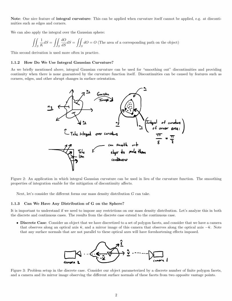
Note: One nice feature of integral curvature: This can be applied when curvature itself cannot be applied, e.g. at disconti-nuities such as edges and corners.

We can also apply the integral over the Gaussian sphere: ZZ ZZ ZZ 1 dO dS = dS = dO = O (The area of a corresponding path on the object)

K dSS S S

This second derivation is used more often in practice.

1.1.2 How Do We Use Integral Gaussian Curvature?

As we briefly mentioned above, integral Gaussian curvature can be used for “smoothing out” discontinuities and providing continuity when there is none guaranteed by the curvature function itself. Discontinuities can be caused by features such as corners, edges, and other abrupt changes in surface orientation.

Figure 2: An application in which integral Gaussian curvature can be used in lieu of the curvature function. The smoothing properties of integration enable for the mitigation of discontinuity affects.

Next, let’s consider the different forms our mass density distribution G can take.

1.1.3 Can We Have Any Distribution of G on the Sphere?

It is important to understand if we need to impose any restrictions on our mass density distribution. Let’s analyze this in both the discrete and continuous cases. The results from the discrete case extend to the continuous case.

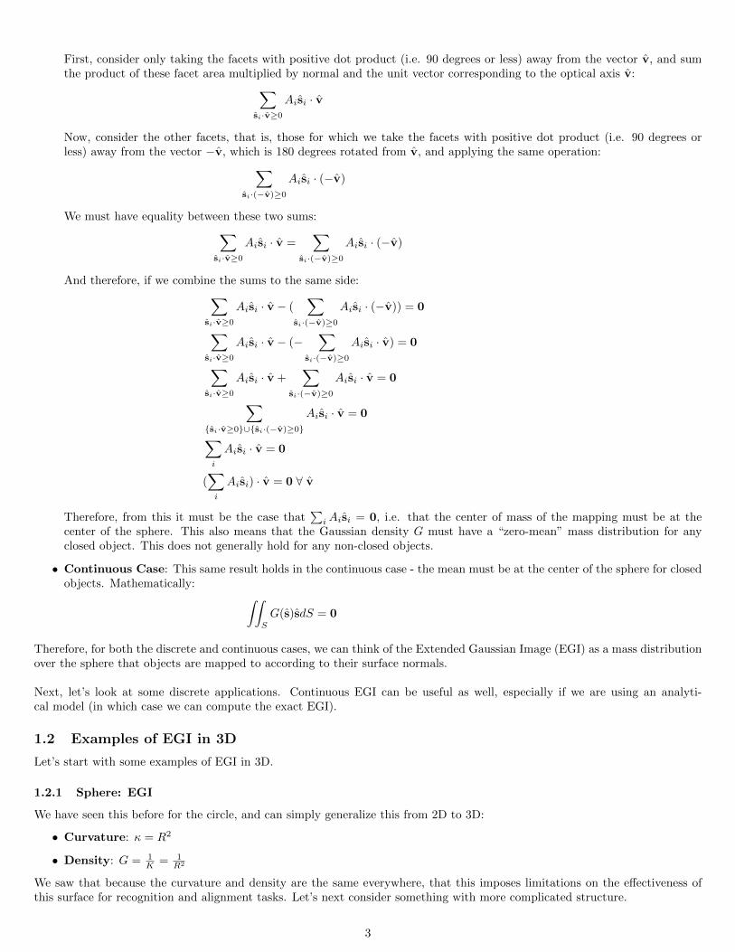
• Discrete Case: Consider an object that we have discretized to a set of polygon facets, and consider that we have a camera that observes along an optical axis v, and a mirror image of this camera that observes along the optical axis −v. Note that any surface normals that are not parallel to these optical axes will have foreshortening effects imposed.

Figure 3: Problem setup in the discrete case. Consider our object parameterized by a discrete number of finite polygon facets, and a camera and its mirror image observing the different surface normals of these facets from two opposite vantage points.

2

First, consider only taking the facets with positive dot product (i.e. 90 degrees or less) away from the vector v, and sum the product of these facet area multiplied by normal and the unit vector corresponding to the optical axis v: X

Aisi · v si ·v≥0

Now, consider the other facets, that is, those for which we take the facets with positive dot product (i.e. 90 degrees or less) away from the vector −v, which is 180 degrees rotated from v, and applying the same operation: X

Aisi · (−v) si ·(−v)≥0

We must have equality between these two sums: X X Aisi · v = Aisi · (−v)

si ·v≥0 si ·(−v)≥0

And therefore, if we combine the sums to the same side: X X Aisi · v − ( Aisi · (−v)) = 0

si ·v≥0 si ·(−v)≥0 X X Aisi · v − (− Aisi · v) = 0

si ·v≥0 si ·(−v)≥0 X X Aisi · v + Aisi · v = 0

si ·v≥0 si ·(−v)≥0 X Aisi · v = 0

{si ·v≥0}∪{si ·(−v)≥0}X Aisi · v = 0

iX ( Aisi) · v = 0 ∀ v

i P Therefore, from this it must be the case that Aisi = 0, i.e. that the center of mass of the mapping must be at thei center of the sphere. This also means that the Gaussian density G must have a “zero-mean” mass distribution for any closed object. This does not generally hold for any non-closed objects.

• Continuous Case: This same result holds in the continuous case - the mean must be at the center of the sphere for closed objects. Mathematically: ZZ

G(s)sdS = 0 S

Therefore, for both the discrete and continuous cases, we can think of the Extended Gaussian Image (EGI) as a mass distribution over the sphere that objects are mapped to according to their surface normals.

Next, let’s look at some discrete applications. Continuous EGI can be useful as well, especially if we are using an analyti-cal model (in which case we can compute the exact EGI).

1.2 Examples of EGI in 3D

Let’s start with some examples of EGI in 3D.

1.2.1 Sphere: EGI

We have seen this before for the circle, and can simply generalize this from 2D to 3D:

• Curvature: κ = R2

1 1• Density: G = K = R2

We saw that because the curvature and density are the same everywhere, that this imposes limitations on the effectiveness of this surface for recognition and alignment tasks. Let’s next consider something with more complicated structure.

3

1.2.2 Ellipsoid: EGI

Recall our two main ways to parameterize ellipses/ellipsoids: implicit (the more common form) and “squashed circle/sphere” (in this case, the more useful form: � �2 � �2 � �2x y z• Implicit parameterization: + + = 1 a b c

• “Sphere Squashing” parameterization: These are parameterized by θ and φ:

x = a cos θ cos φ

y = b sin θ cos φ

z = c sin φ

We will elect to use the second of these representations because it allows for easier and more efficient generation of points by parameterizing θ and φ and stepping these variables.

As we did last time for the 2D ellipse, we can express these parametric coordinates as a vector parameterized by θ and φ:

r = (a cos θ cos φ, b sin θ cos φ, c sin φ)T

And similarly to what we did before, to compute the surface normal and the curvature, we can first find (in this case, two) tangent vectors, which we can find by taking the derivative of r with respect to θ and φ:

rθ = Δ dr

= (−a sin θ cos φ, b cos θ cos φ, 0)T

dθ

rφ = Δ dr

= (−a cos θ sin φ, −b sin θ sin φ, c cos φ)T

dφ

Then we can compute the normal vector by taking the cross product of these two tangent vectors of the ellipsoid. We do not carry out this computation, but this cross product gives:

n = rθ × rφ = cos φ(b cos θ cos φ, ac sin θ cos φ, ab sin φ)T

= (b cos θ cos φ, ac sin θ cos φ, ab sin φ)T

Where we have dropped the cos φ factor because we will need to normalize this vector anyway. Note that this vector takes a similar structure to that of our original parametric vector r.

With our surface normals computed, we are now equipped to match surface normals on the object to the surface normals on the unit sphere. To obtain curvature, our other quantity of interest, we need to differentiate again. We will also change our parameterization from (θ, φ) → (ξ, η), since (θ, φ) parameterize the object in its own space, and we want to parameterize the object in unit sphere space (ξ, η).

n = (cos ξ cos η, sin ξ cos η, sin η)T

s = (a cos ξ cos η, b sin ξ cos η, sin η)T � �2 s · s

κ = abc � �21 abc

G = = K s · s

With the surface normals and curvature now computed, we can use the distribution G on the sphere for our desired tasks of recognition and alignment!

Related, let us look at the extrema of curvature for our ellipsoid. These are given as points along the axes of the ellipsoids: � �2 bc1. a � �2ac2. b � �2 ab3. c

4

For these extrema, there will always be one maxima, one minima, and one saddle point. The mirror images of these extrema (which account for the mirrors of each of these three extrema above) exhibit identical behavior and reside, geometrically, on the other side of the sphere we map points to.

How Well Does this Ellipsoid Satisfy Our Desired Representation Properties?

• Translation invariance: As we saw with EGI last time, this representation is robust to translation invariance.

• Rotation “Equivariance”: This property works as desired as well - rotations of the ellipsoid correspond to equivariant rotations of the EGI of this ellipse.

1.3 EGI with Solids of Revolution

We saw above that the EGI for an ellipsoid is more mathematically-involved, and is, on the other end, “too simple” in the case of a sphere. Are there geometric shapes that lend themselves well for an “intermediate representation”? It turns out there are, and these are the solids of revolution. These include:

• Cylinders

• Spheres

• Cones

• Hyperboloids of one and two sheets

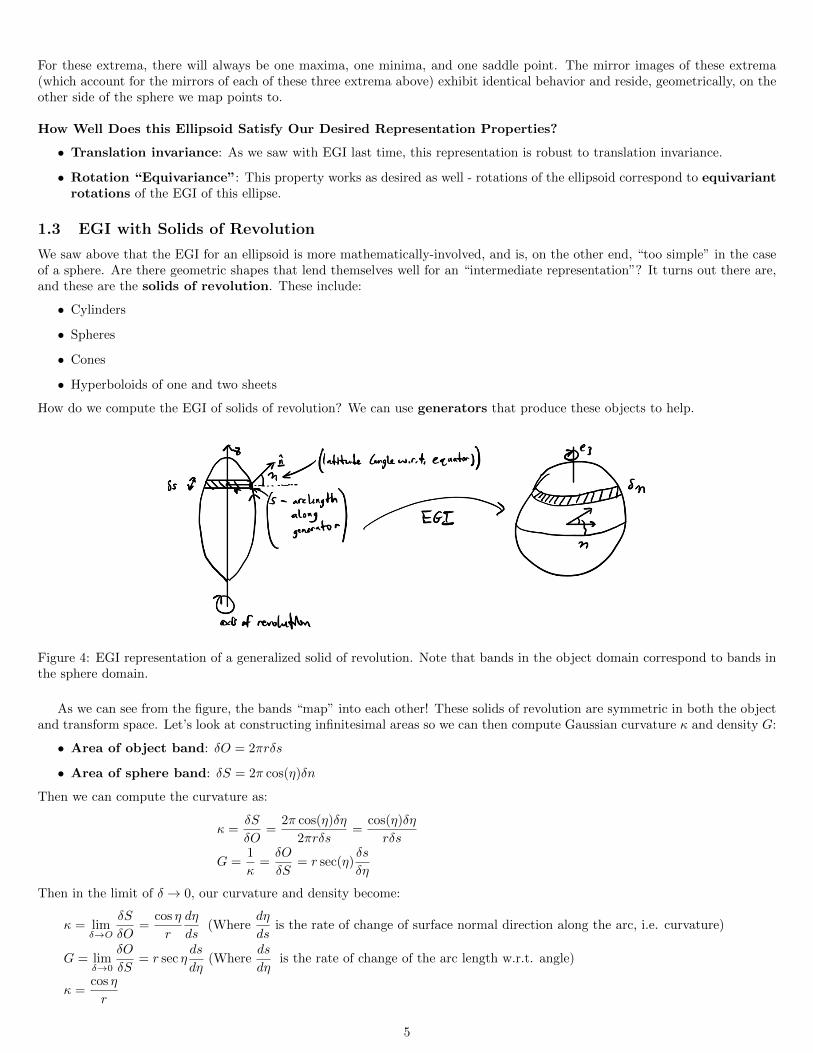
How do we compute the EGI of solids of revolution? We can use generators that produce these objects to help.

Figure 4: EGI representation of a generalized solid of revolution. Note that bands in the object domain correspond to bands in the sphere domain.

As we can see from the figure, the bands “map” into each other! These solids of revolution are symmetric in both the object and transform space. Let’s look at constructing infinitesimal areas so we can then compute Gaussian curvature κ and density G:

• Area of object band: δO = 2πrδs

• Area of sphere band: δS = 2π cos(η)δn

Then we can compute the curvature as:

δS 2π cos(η)δη cos(η)δη κ = = =

δO 2πrδs rδs 1 δO δs

G = = = r sec(η)κ δS δη

Then in the limit of δ → 0, our curvature and density become:

δS cos η dη dη κ = lim = (Where is the rate of change of surface normal direction along the arc, i.e. curvature)

δ→O δO r ds ds δO ds ds

G = lim = r sec η (Where is the rate of change of the arc length w.r.t. angle) δ→0 δS dη dη cos η

κ = r

5

1.4 Gaussian Curvature

Using the figure below, we can read off the trigonometric terms from this diagram to compute the curvature κ in a different way:

Figure 5: Our infinitesimal trigonometric setup that we can use to calculate Gaussian curvature.

We can read off the trigonometric terms as:

−δr sin η = = −rs (First derivative)

δs dη d

cos η = (−rs) = −rss (Second derivative) ds ds

Then the curvature for the solid of revolution is given by:

−rssκ =

r

Let’s look at some examples to see how this framework applies:

1.4.1 Example: Sphere

Take the following cross-section of a sphere in 2D:

R

Figure 6: Cross-section of a 3D sphere in 2D. We can apply our framework above to derive our same result for Gaussian curvature.

Mathematically: � � S

r = R cos R� � � � � � 1 S 1 S

rss = R − cos = − cos R2 R R R

Then curvature is given by: � �� � − 1 S− cos−rss

= 1R� �κ = = R2S

R r R cos

Alternatively, rather than expressing this in terms of R and S, we can also express as a function of z (with respect to the diagram

6

above). Let’s look at some of the quantities we need for this approach:

dr tan η = − = −rz (First derivative)

dz dη d dz2 sec = (−rz ) = −rzz (By Chain Rule)ds ds ds

sec 2 η = 1 + tan2 η

dz cos η = = −zs

dη

Putting all of these equations together:

−rzz κ =

r(1 + z2)2 p r = R2 − Z2

Z rz = −√

R2 − Z2

R2

rzz 3 = − 2(R2 − Z2)

R2 21 + r = z R2 − Z2

−rzz 1 Then: κ = =

r(1 + z2)2 R2

One particular EGI, and the applications associated with it, is of strong interest - the torus.

1.4.2 EGI Example Torus

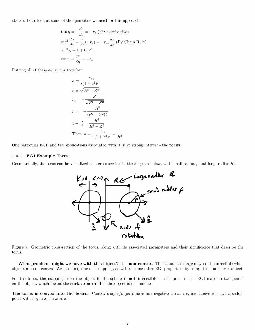
Geometrically, the torus can be visualized as a cross-section in the diagram below, with small radius ρ and large radius R.

Figure 7: Geometric cross-section of the torus, along with its associated parameters and their significance that describe the torus.

What problems might we have with this object? It is non-convex. This Gaussian image may not be invertible when objects are non-convex. We lose uniqueness of mapping, as well as some other EGI properties, by using this non-convex object.

For the torus, the mapping from the object to the sphere is not invertible - each point in the EGI maps to two points on the object, which means the surface normal of the object is not unique.

The torus is convex into the board. Convex shapes/objects have non-negative curvature, and above we have a saddle point with negative curvature.

7

Keeping these potential issues in mind, let’s press on. Mathematically:

r = R + ρ cos η � � S

= R + ρ cos ρ

From here, we can take the second derivative rss: � � d2r 1 s

rss = = − cos ds2 ρ ρ

Combining/substituting to solve for curvature κ: � �

ρS

−rss 1 cos � �κ = = r ρ R + ρ cos ρ

S

We will also repeat this calculation for the corresponding surface normal on the other side. We will see that this results in different sign and magnitude:

r = R − ρ cos η � � S

= R − ρ cos ρ

From here, we can take the second derivative rss: � � d2r 1 s

= = cosrss ds2 ρ ρ

Combining/substituting to solve for curvature κ: � �

ρS

−rss 1 cos � �κ = = − r ρ R + ρ cos ρ

S

Since we have two different Gaussian curvatures, and therefore two separate densities for the same surface normal, what do we do? Let’s dicuss two potential approaches below.

1. Approach 1: Adding Densities: For any non-convex object in which we have multiple points with the same surface normals, we can simply add these points together in density:

1 1 G = + = 2ρ2

κ+ κ−

Even though this approach is able to cancel many terms, it creates a constant density, which means we will not be able to solve alignment/orientation problems. Let’s try a different approach.

2. Approach 2: Subtracting Densities: In this case, let us try better taking into account local curvature by subtracting instead of adding densities, which will produce a non-constant combined density:

1 1 G = − = 2Rρ sec(η)

κ+ κ−

This result is non-constant (better for solving alignment/orientation problems), but we should note that because of the secant term, it has a singularity at the pole. We can conceptualize this singularity intuitively by embedding a sphere within an infinite cylinder, and noting that as we approach the singularity, the mapped location climbs higher and higher on the cylinder.

8

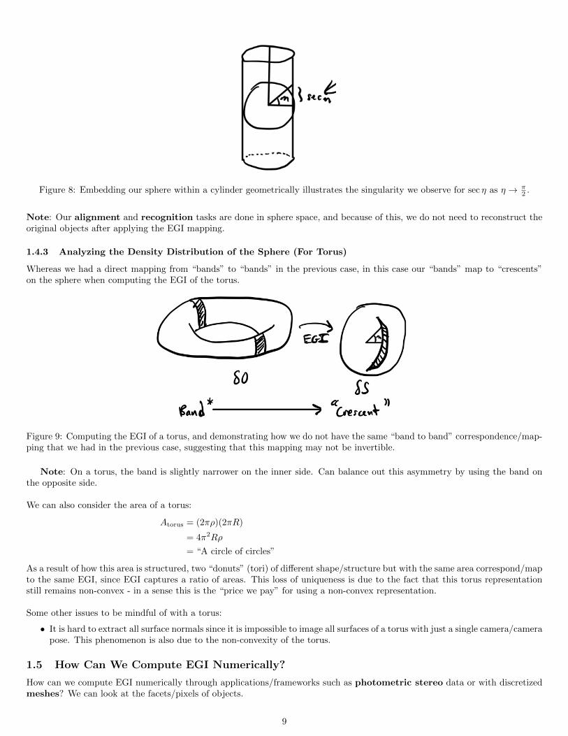
Figure 8: Embedding our sphere within a cylinder geometrically illustrates the singularity we observe for sec η as η → π 2 .

Note: Our alignment and recognition tasks are done in sphere space, and because of this, we do not need to reconstruct the original objects after applying the EGI mapping.

1.4.3 Analyzing the Density Distribution of the Sphere (For Torus)

Whereas we had a direct mapping from “bands” to “bands” in the previous case, in this case our “bands” map to “crescents” on the sphere when computing the EGI of the torus.

Figure 9: Computing the EGI of a torus, and demonstrating how we do not have the same “band to band” correspondence/map-ping that we had in the previous case, suggesting that this mapping may not be invertible.

Note: On a torus, the band is slightly narrower on the inner side. Can balance out this asymmetry by using the band on the opposite side.

We can also consider the area of a torus:

Atorus = (2πρ)(2πR)

= 4π2Rρ

= “A circle of circles”

As a result of how this area is structured, two “donuts” (tori) of different shape/structure but with the same area correspond/map to the same EGI, since EGI captures a ratio of areas. This loss of uniqueness is due to the fact that this torus representation still remains non-convex - in a sense this is the “price we pay” for using a non-convex representation.

Some other issues to be mindful of with a torus:

• It is hard to extract all surface normals since it is impossible to image all surfaces of a torus with just a single camera/camera pose. This phenomenon is also due to the non-convexity of the torus.

1.5 How Can We Compute EGI Numerically?

How can we compute EGI numerically through applications/frameworks such as photometric stereo data or with discretized meshes? We can look at the facets/pixels of objects.

9

Let us first suppose we have a triangular facet:

Figure 10: A triangular facet, which we can imagine we use to compute our EGI numerically.

As we have done before, we can find the surface normal and area of this facet to proceed with our EGI computation:

• Surface Normal: This can be computed simply by taking the cross product between any of the two edges of the triangular facet, e.g.

n = (b − a) × (c − b)

= (a × b) + (b × c) + (c × a)

• Area: This can be computed by recalling the area of a triangular ( 1 base × height): 2

1 A = (b − a) · (c − a)

2 1

= ((a · a + b · b + c · c) − (a · b + b · c + c · a))6

We can repeat this area and surface normal computation on all of our facets/elements to compute the mass distribution over the sphere by adding different facets from all over surface. We add rather than subtract components to ensure we have a non-constant EGI, and therefore have an EGI representation that is suitable for alignment tasks.

1.5.1 Direction Histograms

Direction histograms are another way of thinking about how we build an EGI. These are used in different applications outside of machine vision as well, e.g. finding direction histograms in (i) muscle fibers, (ii) neural images, (iii) analyzing blood vessels.

Typically, these direction histograms can be used to ascertain what the most common orientations are amongst a set of orientations.

For histograms in higher dimensions, is subdividing the region into squares/cubes the most effective approach? As it turns out, no, and this is because the regions are not round. We would prefer to fill in the plane with disks.

To contrast, suppose the tessellation is with triangles - you are now combining things that are pretty far away, compared to a square. Hexagons alleviate this problem by minimizing distance from the center of each cell to the vertives, while also preventing overlapping/not filled in regions. Other notes:

• We also need to take “randomness” into account, i.e. when points lie very close to the boundaries between different bins. We can account for this phenomena by constructing and counting not only the original grids, but additionally, shifted/offset grids that adjust the intervals, and consequently the counts in each grid cell.

The only issue with this approach is that this “solution” scales poorly with dimensionality: As we increase dimensions, we need to take more grids (e.g. for 2D, we need our (i) Original plane, (ii) Shifted x, (iii) Shifted y, and (iv) Shifted x and shifted y). However, in light of this, this is a common solution approach for mitigating “randomness” in 2D binning.

1.5.2 Desired Properties of Dividing Up the Sphere/Tessellations

To build an optimal representation, we need to understand what our desired optimal properties of our tessellations will be:

1. Equal areas of cells/facets

2. Equal shapes of cells/facets

10

3. “Rounded” shapes of cells/facets

4. Regular pattern

5. Allows for easy “binning”: As an example a brute force way to do binning for spheres is to compute the dotr product with all surface normals and take the largest of these. This is very impractical and computationally-inefficient because it requires us to step through all data each time. For this reason, it is important we consider implementations/representations that make binning efficient and straightforward.

6. Alignment of rotation: The idea with this is that we need to bring one object into alignment with the other in order to do effective recognition, one of the key tasks we cited.

For instance, with a dodecahedron, our orientation/direction histogram is represented by 12 numbers (which cor-respond to the number of faces on the dodecahedron):

[A1, A2, · · · , A12]

When we bring this object into alignment during, for instance, a recognition task, we merely only need to permute the order of these 12 numbers - all information is preserved and there is no loss from situations such as overlapping. This is an advantage of having alignment of rotation.

[A7, A4, · · · , A8]

Platonic and Archimedean solids are the representations we will use for these direction histograms.

11

MIT OpenCourseWare https://ocw.mit.edu

6.801 / 6.866 Machine Vision Fall 2020

For information about citing these materials or our Terms of Use, visit: https://ocw.mit.edu/terms