650 ieee transactions on signal …web.eecs.umich.edu/~hero/preprints/cartertsp10.pdf650 ieee...

650 IEEE TRANSACTIONS ON SIGNAL PROCESSING, VOL. 58, NO. 2, FEBRUARY 2010

On Local Intrinsic Dimension Estimation andIts Applications

Kevin M. Carter, Student Member, IEEE, Raviv Raich, Member, IEEE, and Alfred O. Hero III, Fellow, IEEE

Abstract—In this paper, we present multiple novel applicationsfor local intrinsic dimension estimation. There has been muchwork done on estimating the global dimension of a data set, typi-cally for the purposes of dimensionality reduction. We show thatby estimating dimension locally, we are able to extend the uses ofdimension estimation to many applications, which are not possiblewith global dimension estimation. Additionally, we show thatlocal dimension estimation can be used to obtain a better globaldimension estimate, alleviating the negative bias that is commonto all known dimension estimation algorithms. We illustrate localdimension estimation’s uses towards additional applications, suchas learning on statistical manifolds, network anomaly detection,clustering, and image segmentation.

Index Terms—Geodesics, image segmentation, intrinsic dimen-sion, manifold learning, nearest neighbor graph.

I. INTRODUCTION

T ECHNOLOGICAL advances in both sensing and mediastorage have allowed for the generation of massive

amounts of high-dimensional data and information. Considerthe class of applications that generate these high-dimensionalsignals: e.g., digital cameras capture images at enormous reso-lutions; dozens of video cameras may be filming the exact sameobject from different angles; planes randomly drop hundredsof sensors into the same area to map the terrain. While this hasopened a wealth of opportunities for data analysis, the problemof the curse of dimensionality has become more substantial, asmany learning algorithms perform poorly in high dimensions.While the data in these applications may be represented inhigh dimensions, strictly based upon the immense capacity fordata retrieval, it is typically concentrated on lower dimensionalsubsets—manifolds—of the measurement space. This allowsfor significant dimension reduction with minor or no loss ofinformation. The point at which the data can be reduced with

Manuscript received November 05, 2008; accepted July 20, 2009. First pub-lished September 09, 2009; current version published January 13, 2010. Theassociate editor coordinating the review of this manuscript and approving it forpublication was Prof. Cedric Richard. This work was supported in part by theNational Science Foundation under Grant CCR-0325571.

K. M. Carter was with the Department of Electrical Engineering and Com-puter Science, University of Michigan, Ann Arbor, MI 48109 USA (e-mail:[email protected]).

R. Raich is with the School of Electrical Engineering and Computer Sci-ence, Oregon State University, Corvallis, OR 97331 USA (e-mail: [email protected]).

A. O. Hero III is with the Department of Electrical Engineering and Com-puter Science, University of Michigan, Ann Arbor, MI 48109 USA (e-mail:[email protected]).

Digital Object Identifier 10.1109/TSP.2009.2031722

minimal loss is related to the intrinsic dimensionality of themanifold supporting the data. This measure may be interpretedas the minimum number of parameters required to describe thedata [1].

When the intrinsic dimension is assumed constant over thedata set, several algorithms [2]–[5] have been proposed to es-timate the dimensionality of the manifold. In several problemsof practical interest, however, data will exhibit varying dimen-sionality, as there may lie multiple manifolds of varying dimen-sion within the data. This is easily viewed in images with dif-ferent textures or in classification tasks in which data from dif-ferent classes is generated by unique probability density func-tions (pdfs). In these situations, the local intrinsic dimensionmay be of more importance than the global dimension. In pre-vious work [6], we illustrated the process of local dimensionestimation, in which a dimension estimate is obtained for eachsample within the data, rather than a single dimension estimatefor the entire set.

In this paper, we focus on the applications of local dimen-sion estimation. One immediate benefit is using local dimensionto estimate the global dimension of a data set. To our knowl-edge, every method of estimating intrinsic dimension has ex-pressed an issue with a negative bias. While insufficient sam-pling is a common source of this bias, a significant portion isa result of samples near the boundaries or edges of a mani-fold. These regions appear to be low dimensional when sampledand contribute a strong negative bias to the global estimate ofdimension. We additionally utilize local dimension estimationfor the purposes of dimensionality reduction. Typically, this hasbeen presented for Riemannian manifolds in a Euclidean space[7]–[9], in which the data contain a single manifold of constantdimension lying in . We extend this to the problem of estima-tion and reduction of dimensionality on statistical manifolds, inwhich the points on the manifold are pdfs rather than points ina Euclidean space.

We continue by showing novel applications in which the exactdimension of the data is of no immediate concern, but rather thedifferences between the local dimensions. Dimensionality canbe viewed as the number of degrees of freedom in a data set, andas such may be interpreted as a measure of data complexity. Bycomparing the local dimension of samples within a data set, weare able to identify different subsets of the data for analysis. Forexample, in a time-series data set, the intrinsic dimensionalitymay change as a function of time. By viewing each time step asa sample, we can identify changes in the system at specific timepoints. We illustrate this ability by finding anomalous activityin a router network. Additionally, the identification of subsets

1053-587X/$26.00 © 2010 IEEE

Authorized licensed use limited to: Alfred Hero. Downloaded on March 20,2010 at 17:54:42 EDT from IEEE Xplore. Restrictions apply.

CARTER et al.: ON LOCAL INTRINSIC DIMENSION ESTIMATION AND ITS APPLICATIONS 651

within the data allows for the immediate application of clus-tering and image segmentation. There has been much work pre-sented on using fractal dimension estimation for image and tex-ture segmentation [10], [11]. In this paper, we do not make themodel assumption that textures may be represented as a collec-tion of fractals [12], and instead segment images using a novelmethod based on Euclidean dimension. We show that by using“neighborhood smoothing” [13] over the dimension estimates,we are able to find the regions that exhibit differing complexi-ties, and use the smoothed dimension estimates as identifiers forthe clusters/segments.

The organization of this paper is as follows: We give anoverview of the two dimension estimation algorithms we willutilize in our simulations in Section II. In Section III, wedescribe the process of neighborhood smoothing as a meansof postprocessing for local dimension estimation. We illustratethe various novel applications of local dimension estimationin Section IV, including debiasing for global dimension esti-mation, manifold learning, anomaly detection, clustering, andimage segmentation. Lastly, we offer a discussion and presentareas for future work in Section V.

II. DIMENSION ESTIMATION

We will now present two algorithms for dimension estima-tion: the -nearest neighbor ( -NN) algorithm [4], [14] and themaximum likelihood estimator (MLE) method [5]. Please notethat this paper makes no attempts to claim superiority of thesealgorithms over others. While there are many algorithms avail-able for dimension estimation, we focus on these two as a meansfor illustrating the applications we later present. By utilizing twodistinct methods, we hope to quell any concerns that our appli-cations are algorithm dependent. For a thorough survey of in-trinsic dimension estimation methods, we encourage the readerto view [15] and [16], as well as more recent work [17]–[20].

A. The -Nearest Neighbor Algorithm for DimensionEstimation

Let be independent identically dis-tributed (i.i.d.) random vectors with values in a compact subsetof . The (1-)nearest neighbor of in is given by

where is an appropriate distance measure betweenand ; for the purposes of this paper, let us define

, the standard Euclidean distance. For a generalinteger , the -nearest neighbor of a point is defined ina similar way. The -NN graph assigns an edge between eachpoint in and its -nearest neighbors. Letbe the set of -nearest neighbors of in . The total edgelength of the -NN graph is defined as

(1)

where is a power weighting constant.For many data sets of interest, the random vectors are

constrained to lie on an -dimensional Riemannian submani-

fold of . Under this framework, the asymptoticbehavior of (1) is given as

(2)

where is a constant with respect tothat depends on the Rényi entropy of the distribution of

the manifold and is an error residual [6]. Note that for easeof notation, we will denote simply as , except where theexplicit expression is desirable (e.g., optimizing over ).

As noisy measurements can lead to inaccurate estimates, theintrinsic dimension should be estimated using a nonlinearleast squares solution. By calculating sampled graph lengthsover varying values of , the effect of noise can be dimin-ished. In order to calculate graph lengths for differing samplesizes on the manifold, it is necessary to randomly subsamplefrom the full set , utilizing the nonoverlap-ping block bootstrapping method [21]. Specifically, let

be a spatially or temporally sorted version of, and let be an integer satisfying . Define the

blocks . Assuch, we may now redefine .

Let be integers such that. For each value of , randomly draw

bootstrap datasets , with replacement,where the blocks of data points within each are chosenfrom the entire data set independently. From these samples,define , where .

Since is dependent on , it is necessary to solve for theminimum mean squared error, derived from (2), by minimizingover both and integer values of

(3)

where and is the vector of length whose elementsare all one. We solve over integer values of , as we do notconsider fractal dimensions for this algorithm. This improvesaccuracy by constraining the estimation space to discrete valuesrather than discretizing estimates in a continuous space. One cansolve (3) in the following general manner.

1: Calculate from the expansion of (3)a)

2: Calculate the error with and from step 1)

.

This nonlinear least squares solution yields the dimension es-timate based on the -NN graphs.

B. The Maximum Likelihood Estimator for Intrinsic Dimension

The MLE method [5] for dimension estimation estimates theintrinsic dimension from a collection of i.i.d. observations



. Similar to the -NN algo-rithm for dimension estimation, the MLE method assumes thatclose neighbors lie on the same manifold. The estimator pro-ceeds as follows, letting be a fixed number of nearest neigh-bors to sample

(4)

where is the distance from point to its th nearestneighbor in . The intrinsic dimension for the data set can thenbe estimated as the average over all observations

Algorithm 1: Local dimension estimation

Input: Data set1: for to do2: Initialize cluster3: for to4: Find the th NN, , of5:6: end for7:8: end for

Output: Local dimension estimates for

C. Local Dimension Estimation

While the MLE method inherently generates local dimensionestimates for each sample , the -NN algorithm in itselfis a global dimension estimator. We are able to adopt it (andany other dimension estimation algorithm) as a local dimen-sion estimator by running the algorithm over a smaller neigh-borhood about each sample point. Define a set of samples

from the collection of manifoldssuch that each point lies on manifold .

Any small sphere or data cluster of samples centeredat point , with , will contain samples from

distinct manifolds. As , all of the pointsin will lie on a single manifold (i.e., ). Intuitivelyspeaking, as the cluster about point is reduced in size, thelocal neighborhood defined by said cluster can be viewed as itsown data set confined to a single manifold. Hence, we can usea global dimension estimation algorithm on a local subset ofthe data to estimate the local intrinsic dimension of each samplepoint. This can be performed as described in Algorithm 1, where“dimension ” refers to applying any method of dimension es-timation to the data cluster .

One of the keys to local dimension estimation is defining avalue of . There must be a significant number of samples inorder to obtain a proper estimate, but it is also important to keepa small sample size as to (ideally) only include samples that lieon the same manifold. Currently, we arbitrarily choose basedon the size of the data set. However, a more definitive methodof choosing is grounds for future work.

We briefly note that our definition of “local” dimensionestimation differs from that of the Fukunaga–Olsen algorithm

[1]. Specifically, we aim to find a dimension estimate for eachsample point, which accounts for sets consisting of multiplemanifolds, while [1] used local subsets of the data to form aglobal estimate of dimension.

III. NEIGHBORHOOD SMOOTHING

For the problem of local dimension estimation, results areoften highly variable, where nearby samples from the samemanifold may result in different dimension estimates. This issuecan be a result of a variety of reasons, such as variability dueto random subsampling in the -NN algorithm, or variabilitydue to the neighborhood size in the MLE method. When con-structing a global dimension estimate, this variance is relativelyinsignificant, as the estimate is constructed as a function of thelocal estimates. For local dimension estimation, however, thisvariance is of significant concern, and we propose a variancereduction method known as neighborhood smoothing [13],which improves estimation accuracy.

An initial intuition for manifold learning algorithms is thatsamples that are “close” tend to lie on the same manifold,which extends to the assumption that they therefore have thesame dimension. With this assumption in place, it followsthat filtering by majority vote over the dimension estimatesof nearby samples should smooth the estimator and reducevariance. This voting strategy is similar to the methods ofmode filtering, bagging [22] and learning by rule ensembles[23]. Smoothing simply looks at the distribution of dimensionestimates within each sample point’s local neighborhood andreassigns each sample a dimension estimate equal to that withthe highest probability within its neighborhood. Specifically

(5)

where is the probability over the neighborhood of the cur-rent sample . Given a finite number of samples ,this may be empirically evaluated as

(6)

where is the standard indicator function. This process maythen be iterated until the set converges such that each estimateremains constant. This has the effect of implicitly incorporatingthe neighbors of each sample’s neighbors to some extent, as thedimension estimates within a local region may change throughiterations.

Intuitively, neighborhood smoothing is similar to itera-tively imposing a -NN classifier on the local dimensionestimates—under the guise that at each iteration, sampleis a test sample and all points are appropriatelylabeled training samples. Similarly to -NN classification, thekey factor to smoothing is defining the neighborhood . If

is too large, oversmoothing will occur. The variance of thedimension estimates will drastically decrease, but there willbe a strong bias which will remove the detection of coarselysampled manifolds. As such, one cannot use a constant regionabout a point but must adapt that region to the statistics of thesample.



A. Adaptive Neighborhood Selection

Since the number of sample points on each manifold of adata set is generally unknown, using a constant number ofsmoothing samples is not a viable option; samples on a smallermanifold may have points from a disjoint manifold includedin their smoothing neighborhood. One straightforward methodfor neighborhood selection is to define neighbors by somespherical region or -ball about each sample point. This isgenerally acceptable when the disjoint manifolds are easilyseparable, as the neighborhood does not adapt to the geometryof the manifold. When distinct manifolds lie near one another,or potentially intersect, it is necessary to further adapt thesmoothing neighborhood beyond a spherical region. This is dueto the fact that points on a nearby or intersecting manifold maybe as close (or closer) to a sample as others on its own manifold.A spherical region may smooth over different manifolds, andthe results will lead to the dimension estimates’ “leaking” fromone manifold to another.

Rather than defining neighborhoods through Euclidean dis-tance, which will form only spherical regions about each samplepoint, we will define neighborhoods using a geodesic distancemetric. This will adapt the neighborhood to the geometry of themanifold. The geodesic distance is defined as the shortest pathbetween two points along the manifold and may be approxi-mated with graph-based methods. For our purposes, this metriccan be determined by taking each point and creating an edge toits -NN. Then, using Dijkstra’s shortest path algorithm (or anyother algorithm for computing the shortest path), approximatethe geodesic distances between each pair of points in the graph.Any points that remain unconnected are considered to have aninfinite geodesic distance between them.

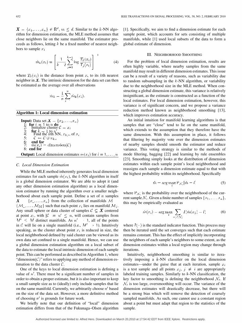
To define a local neighborhood, we can now simply choosethe closest points for which the geodesic distance is not infi-nite. This forms a nonspherical neighborhood that adapts to thecurvature of the manifold, performing much better than spher-ical neighborhoods. Fig. 1 illustrates the difference in the neigh-borhoods (black stars) that are formed on the “swiss roll” man-ifold when using different proximity metrics. The Euclideandistance [Fig. 1(a)] forms a spherical neighborhood, includingpoints that are separated from the sample in question (red di-amond). The geodesic distance [Fig. 1(b)], however, forms aneighborhood considering points only in close proximity alongthe actual manifold. While all points in this example do existon the same manifold, it is clear that defining neighborhoodsalong the manifold rather than in simple spherical regions re-duces the probability of including samples from a nearby dis-tinct manifold.

Illustrating the effects of neighborhood smoothing, we createa seven-dimensional data set that includes two distinct hyper-spheres of intrinsic dimensions two and five, each containing300 uniformly sampled points intersecting in three common di-mensions. Fig. 2(a) shows the histogram of the local dimensionestimates of each sample before any neighborhood smoothingwas applied, while Fig. 2(b) shows the results after smoothing.One can clearly see that the wide histogram was correctly con-densed to the proper local dimension estimates, even though the

Fig. 1. Neighborhoods �� of the sample in question �� defined by(a) Euclidean distance and (b) geodesic distance. (a) Spherical neighborhoodand (b) adaptive neighborhood.

manifolds intersect. The use of the geodesic distance measureprevents smoothing across distinct manifolds, which lie closelytogether in Euclidean space.

It is important to note that, as with any form of postpro-cessing, neighborhood smoothing can only produce accurateresults given sufficient input. The benefits of smoothing canbe significantly diminished if the initial local dimension esti-mates are not sufficiently accurate. We note this explicitly be-cause of the known issues with estimating large dimensions(e.g., ). Because of variance issues due to insufficientsamples and boundary effects, it is difficult to accurately esti-mate very large dimensions, and often the estimate can moreappropriately be considered a measure of complexity, where thedifference between and 1 is rather insignificant. This isimportant because no single dimension may dominate a givenlocal neighborhood, yet smoothing will still assign a dimen-sion estimate equal to the most represented dimension, whichmay indeed be inconsistent with the rest. We demonstrate thisscenario with the example shown in Fig. 3, where smoothingwould assign a dimension estimate of , which is themost represented dimension in the neighborhood. However, amore accurate dimension estimate could be consideredor , as that would be more consistent with the majorityof the samples. In these scenarios, it may be more appropriateto smooth over a histogram with user-defined bin sizes, corre-sponding to significant differences in complexity rather than in-dividual dimensions. This is an area for future work.



Fig. 2. Neighborhood smoothing applied to seven-dimensional data containingtwo spheres with intrinsic dimensions two and five.

Fig. 3. Issues arise with neighborhood smoothing when estimating very largedimensions due to the variance of such estimates. In this example, smoothingwould assign a dimension estimate of 40, although the more appropriate esti-mate would be 33 or 34.

IV. APPLICATIONS

A. Debiasing Global Dimension Estimation

To our knowledge, a phenomenon common to all algorithmsof intrinsic dimension estimation is a negative bias in the di-

Fig. 4. PDFs of data depth based on estimated intrinsic dimension. Points withless depth estimate at a lower dimension, contributing to the overall negativebias.

mension estimate. It is believed that this is an effect of under-sampling the high-dimensional manifold. While the bias due tolack of sufficient samples is inherent, we offer that the samplesize is not the only source of bias; a significant portion is relatedto the depth of the data. Specifically, as data samples approachthe boundaries of the manifold, they exhibit a lower intrinsic di-mension. This issue becomes more prevalent as the dimensionof the manifold increases and is directly related to the curse ofdimensionality. Note that even manifolds that appear “empty” intheir extrinsic-dimensional space (e.g., the Swiss roll) are filledand contain boundaries in the space of their intrinsic dimension.

Previous work [24] has demonstrated that as dimensionalityincreases, the nearest neighbor distances approach those of themost distant points; this will clearly have an adverse effect onneighborhood-based estimation algorithms. We are able to fur-ther correlate this effect on dimension estimation by calculatingthe depth of each sample and quantitatively analyzing the rela-tionship between depth and dimension. We utilize the -datadepth algorithm developed in [25], which calculates depth

as the sum of all the unit vectors between the sample ofinterest and the rest of the data set .Specifically

(7)

where is the unit vector inthe direction of . This depth measure assigns the mostinterior points in the data set a depth value approaching one,while samples along the boundaries approach a depth of zero.

Using this measure, we illustrate the effect of data depth ondimension estimation in Fig. 4. The data set used was of 3000points uniformly sampled on a six-dimensional hypercube. Weutilize the MLE method for dimension estimation, and Fig. 4 il-lustrates the distribution of data depths for samples that estimateat different dimensions. It is clear that as the depth increased, sodid the probability of estimating at a higher dimension, even to



the point where the most deep points estimated at a dimensionof seven (although we note that there were very few points withthis estimate).

When estimating the global dimension of a data set, one cansubstantially reduce the negative bias by placing more emphasison the local dimension of those points away from the bound-aries, as they are more indicative of the true dimension of themanifold. Specifically, let the global dimension be estimated asfollows:

(8)

where is a weighting on each sample point. We offer twopotential definitions of , the first being a binary weighting

otherwise(9)

where and is the data depth of thedeepest point. Essentially this binary weight amounts

to debiasing by averaging over the local dimension estimatesof the deepest % of points, where the threshold isuser defined. This is worthwhile for potentially large data sets,where there are enough samples to ignore a large portion ofthem. When this is not the case, let us make the definition

(10)

where is a user-defined constant. This weighting may beviewed as a heat kernel, in which larger depths will yield higherweights. Unlike the binary weighting, which will ignore a largenumber of the data samples, this heat kernel weighting willutilize all samples (even those lying on a boundary) yet givepreference to those with more depth in the manifold.

We now illustrate this debiasing ability in Fig. 5, in whichwe estimated the global dimension of the six-dimensional hy-percube (3000 i.i.d. samples) over 200 unique trials. Fig. 5(a)shows the histogram of biased dimension estimates obtained byusing the entire set for dimension estimation, while Fig. 5(b) es-timates the correct global dimension each trial by using our de-biasing method (8) with the binary weighting function (9) using

.To study the number of samples necessary to accurately es-

timate global dimension, we plot estimation results in Fig. 6.In this simulation, we plot the mean de-biased andunrounded dimension estimated over a 20-fold cross validation,based on differing number of samples on the six-dimensionalhypercube. We can see that if rounded to the nearest integer,the debiased estimate will be correct on average with roughly2500 samples. On the contrary, without debiasing, the estima-tion maintains a much stronger negative bias, never correctlyestimating the dimension when rounded.

It is important to note that our method of debiasing is onlyapplicable for data with a relatively low intrinsic dimension.When dealing with very high dimensional data, the probability

Fig. 5. Developing a debiased global dimension estimate by averaging overthe 50% of points with the greatest depth on the manifold. (a) Biased resultsand (b) debiased results.

Fig. 6. Analysis of how many samples are necessary to appropriately estimatedebiased global dimension. Plot shows mean dimension estimated over a 20-foldcv, with error bars at one standard deviation.

of a sample lying near a boundary approaches one, and thevalue of the depth approximation becomes irrelevant. This isshown in Fig. 7 where the “deepest” and most “shallow” sam-ples converge to the same depth value as the intrinsic dimensionincreases.



Fig. 7. As the intrinsic dimension increases, the maximum and minimum datadepth of points in the set converge to the same value. This simulation was overa fivefold cross-validation with 400 uniformly sampled points on the unit cube.

Prior work on estimating dimension through vector quanti-zation [20] has reported robustness to negative bias. While notoffering a distinct claim or proof of this robustness, the au-thors mention their algorithm obtains larger estimates for high-dimensional data than neighborhood-based methods. Theoreti-cally, this method will suffer from similar bias issues due to theintrinsic geometry of the data, which is not explicitly accountedfor in [20]. The improved performance reported is likely due tothe cross-validation implemented. That said, the use of quan-tization error may indeed be more robust to negative bias thanneighborhood-based methods, and this potential gain is worthfurther investigation.

B. Statistical Manifold Learning

Of particular interest in manifold learning is the intrinsic di-mension to which one can reduce the dimensionality of a dataset with minimal loss of information. This is typically presentedfor data that lie on a Riemannian submanifold of Euclideanspace. We extend this application to the problem of learningon statistical manifolds [26], in which each point on the mani-fold is a pdf. Rather than defining distance with Euclidean met-rics, we approximate the Fisher information distance—with theKullback–Leibler divergence and Hellinger distance—which isthe natural metric on statistical manifolds [27]. We illustratethe use of local dimension estimation in these learning tasksfor the applications of flow cytometry analysis and documentclassification.

1) Flow Cytometry Analysis: In clinical flow cytometry,pathologists gather readings of fluorescent markers and lightscatter off individual blood cells from a patient sample, leadingto a characteristic multidimensional distribution that, de-pending on the panel of markers selected, may be distinct for aspecific disease entity. The data from clinical flow cytometrycan be considered multidimensional both from the standpointof multiple characteristics measured for each cell, and fromthe standpoint of thousands of cells analyzed per sample. In

previous work [28], [29], we have shown the ability to derivean information embedding of the statistical manifold definedby the space of pdfs, in which each patient’s blood sample canbe considered a realization of a pdf on said manifold. We devel-oped Fisher information nonparametric embedding (FINE) asan information geometric method of dimensionality reductionbased on Fisher information distances between pdfs [26].Using FINE, we are able to embed the pdf realizations intoa low-dimensional Euclidean space, in which each patient isrepresented by a single low-dimensional vector. In order todetermine the dimension for this embedding space, we firstapply local dimension estimation to find the desired dimensionof our embedding space.

Let be a collection of data sets wherecorresponds to the flow cytometer output of the th patient.

For our analysis, each patient has either chronic lymphocyticleukemia or mantle cell lymphoma, which display similarcharacteristics with respect to many expressed surface antigensbut are generally distinct in their patterns of expression of twocommon B lymphocyte antigens CD23 and FMC7. We areinterested in the intrinsic dimension of the statistical manifold,realized by , as that is what we plan to embed. We definethe dissimilarity matrix , where is the symmetricKullback–Leibler divergence approximation of the Fisher in-formation distance between pdf estimates on and [30].For this simulation, we estimated the pdfs with kernel densityestimation methods, although any nonparametric method willsuffice. By redefining our local dimension estimation algo-rithms to take the high-dimensional distance matrix—in thespace of pdfs—as an input (which is not an issue, as both the

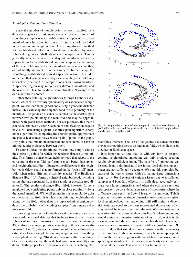
-NN and MLE methods are entirely based on nearest neighbordistances), we are able to estimate the intrinsic dimension ofthe statistical manifold. The local dimension estimation resultsare shown in Fig. 8, where we can see the intrinsic dimensionis . This result can be interpreted as recognizingthe two specific markers that most significantly differentiatebetween classes (i.e., ) but also accounting for the factthat there still exist subtle differences between members of thesame class, and some patients may not exhibit the expectedresponse to specific antigens as strongly as others (i.e., ).

After estimating the intrinsic dimension of the data set, weare able to embed each patient into an -dimensional Euclideanspace, as observed in Fig. 9. In this embedding, each point rep-resents a single patient data set, which was originally six-dimen-sional with samples on the order of . We can see thata two-dimensional unsupervised embedding gives a clear classseparation, which enables effective clustering and classificationof the data. This result is consistent with our dimension estimateof and illustrates the effectiveness of local dimensionestimation for learning on statistical manifolds.

2) Document Classification: Given a collection of docu-ments of known class, we wish to best classify a document ofunknown class. A common representation of a document isknown as the term frequency representation. This is essentiallya normalized histogram of word counts within the document.Specifically, let be the number of times term appears ina specific document. The pdf of that document can then becharacterized as the multinomial distribution of normalized



Fig. 8. Histogram of local dimension estimates for the statistical manifolddefined by flow cytometry results of 43 patients with chronic lymphocyticleukemia or mantle cell lymphoma. (a) Local �-NN dimension estimates and(b) local MLE dimension estimates.

Fig. 9. The information-based embedding, determined by FINE, of the flowcytometry data set. Embedding into � � � dimensions yields linear separa-bility between classes.

word counts, with the maximum likelihood estimate providedas

(11)

Fig. 10. Comparison of (a) pdf of local dimension estimates and (b) classifi-cation rate versus embedding dimension for the 20 Newsgroups data set. Theoptimal embedding dimension ranges from 20 to 50, which is in the same rangeas the apex of the local dimension estimation pdf.

For our illustration, we utilized the 20 Newsgroups1 data set,which has an extrinsic dimension of , which is thenumber of terms in its dictionary. This set contains postingsfrom 20 separate newsgroups, and we wish to classify themby their highest domain (one of [comp.*, rec.*, sci.*, talk.*]).To perform this classification task, we first wish to alleviate thecurse of dimensionality by reducing the data to a lower dimen-sional manifold. For this task we utilize FINE, approximatingthe Fisher information distance with the Hellinger distance, suchthat

where is the estimate (11) of the pdf of document .Experimental results have shown there are multiple subman-

ifolds of differing dimension in the data set. In Fig. 10, wepresent the distribution of dimension estimates and comparethat to classification performance at reduced dimension. Specif-ically, we used the MLE method with the matrix of Hellingerdistances (between full-dimensional pdfs) to estimate the local

1http://people.csail.mit.edu/jrennie/20 Newsgroups/.



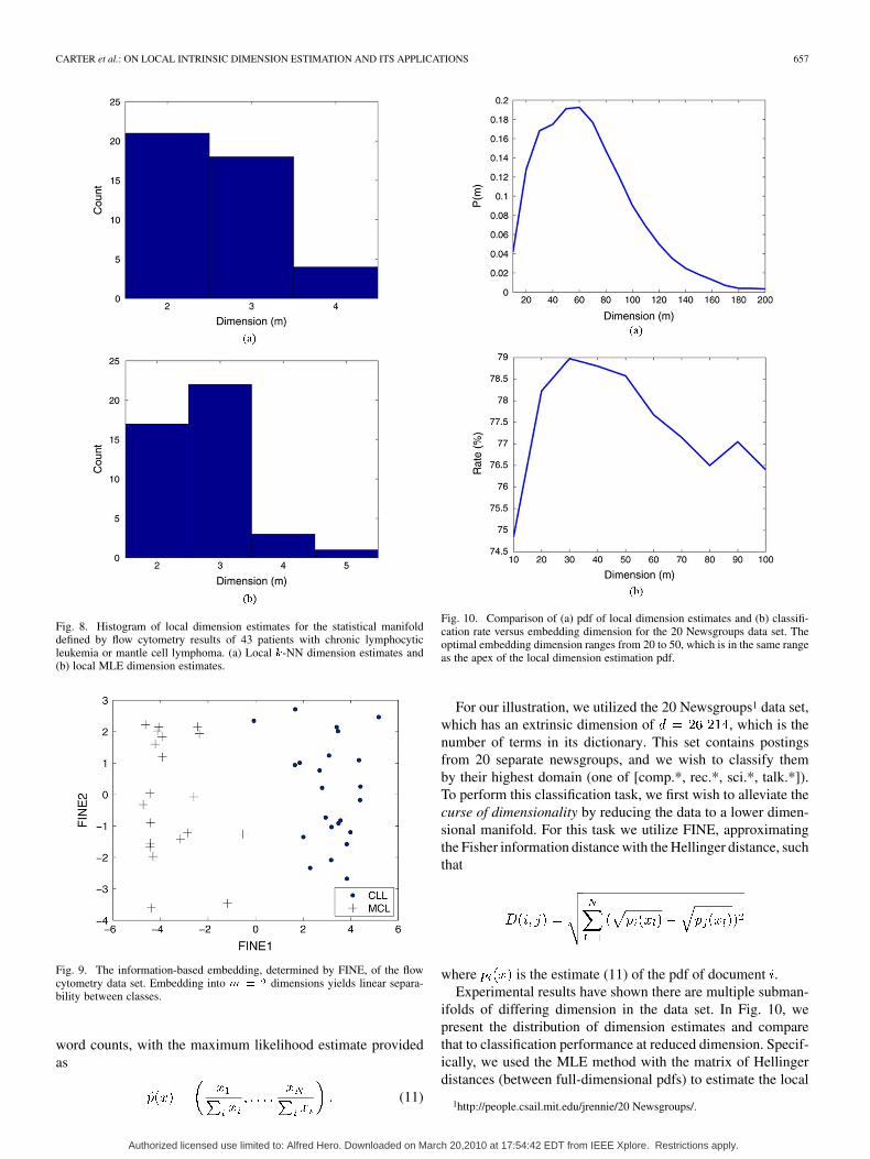
dimension of each sample, then used FINE to embed a randomsubsampling of 1000 points of the data into a lower dimen-sion. The distribution of these local dimension estimates overa 20-fold cross-validation is shown in Fig. 10(a). Next, we sep-arated the embedded data into a training set of 800 samples anda test set of 200 samples. Results of the linear, “all vs. all” classi-fication task (i.e., classify each test sample as one of 4 differentpotential classes) are shown in Fig. 10(b) as a function of theembedding dimension (over the same 20-fold cross-validation).

We observe that the apex of the classification rate curvecorresponds to the apex of the pdf curve of local dimen-

sion estimates , which illustrates that the localdimension estimation method was able to find an appropriateembedding dimension. Although the range seemsto be large, it is important to remember the extrinsic dimensionof the data is , so we are able to adequately definethe dimension of the manifold. We note that for this simulation,we did not utilize neighborhood smoothing due to the high-di-mensional nature of the data, as previously explained. A pdf ofthe local dimension estimates is more beneficial towards anal-ysis than arbitrarily setting a dimension that does not dominatethe neighborhood.

C. Network Anomaly Detection

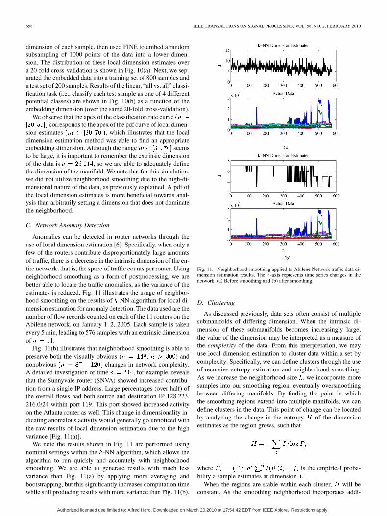
Anomalies can be detected in router networks through theuse of local dimension estimation [6]. Specifically, when only afew of the routers contribute disproportionately large amountsof traffic, there is a decrease in the intrinsic dimension of the en-tire network; that is, the space of traffic counts per router. Usingneighborhood smoothing as a form of postprocessing, we arebetter able to locate the traffic anomalies, as the variance of theestimates is reduced. Fig. 11 illustrates the usage of neighbor-hood smoothing on the results of -NN algorithm for local di-mension estimation for anomaly detection. The data used are thenumber of flow records counted on each of the 11 routers on theAbilene network, on January 1–2, 2005. Each sample is takenevery 5 min, leading to 576 samples with an extrinsic dimensionof .

Fig. 11(b) illustrates that neighborhood smoothing is able topreserve both the visually obvious ( ) andnonobvious changes in network complexity.A detailed investigation of time , for example, revealsthat the Sunnyvale router (SNVA) showed increased contribu-tion from a single IP address. Large percentages (over half) ofthe overall flows had both source and destination IP 128.223.216.0/24 within port 119. This port showed increased activityon the Atlanta router as well. This change in dimensionality in-dicating anomalous activity would generally go unnoticed withthe raw results of local dimension estimation due to the highvariance [Fig. 11(a)].

We note the results shown in Fig. 11 are performed usingnominal settings within the -NN algorithm, which allows thealgorithm to run quickly and accurately with neighborhoodsmoothing. We are able to generate results with much lessvariance than Fig. 11(a) by applying more averaging andbootstrapping, but this significantly increases computation timewhile still producing results with more variance than Fig. 11(b).

Fig. 11. Neighborhood smoothing applied to Abilene Network traffic data di-mension estimation results. The �-axis represents time series changes in thenetwork. (a) Before smoothing and (b) after smoothing.

D. Clustering

As discussed previously, data sets often consist of multiplesubmanifolds of differing dimension. When the intrinsic di-mension of these submanifolds becomes increasingly large,the value of the dimension may be interpreted as a measure ofthe complexity of the data. From this interpretation, we mayuse local dimension estimation to cluster data within a set bycomplexity. Specifically, we can define clusters through the useof recursive entropy estimation and neighborhood smoothing.As we increase the neighborhood size , we incorporate moresamples into our smoothing region, eventually oversmoothingbetween differing manifolds. By finding the point in whichthe smoothing regions extend into multiple manifolds, we candefine clusters in the data. This point of change can be locatedby analyzing the change in the entropy of the dimensionestimates as the region grows, such that

where is the empirical proba-bility a sample estimates at dimension .

When the regions are stable within each cluster, will beconstant. As the smoothing neighborhood incorporates addi-



Fig. 12. The entropy of the local dimension estimates changes as a function ofneighborhood size �.

tional manifolds, the entropy will leave its constant state andeventually as (i.e., the region includes everypoint). With a priori knowledge of the distribution of dimen-sionality, one may choose a neighborhood size that yields anappropriate value of entropy. Without this knowledge, the pointat which leaves its constant state can be used as a thresholdfor defining clusters based on dimension. This process is sim-ilar to dual-rooted diffusion kernels method of clustering [31],in which the authors used the jump in nearest neighbor distanceas a means to differentiate clusters.

For example, let , where isuniformly distributed in [0,1] ( , a discrete set ofinteger values) and constant elsewhere. Hence, is the in-trinsic dimension of . For our simulation, let and

, and there are samples for each value in. After obtaining local dimension estimates, we apply neigh-

borhood smoothing to differing neighborhood sizes and mea-sure the entropy of the local dimension estimates at each size.The results are shown in Fig. 12, where the entropy exhibits thesame pattern we previously described; after initially decreasing,

remains constant as approaches the region size of each man-ifold . As the smoothing covers multiple manifolds

, the entropy decreases until the smoothing neighbor-hood eventually covers all manifolds simultaneously and

. The histogram of local dimension estimates (with both -NNand MLE methods), which is used to calculate the entropy, isshown in Fig. 13 to illustrate the evolution of the dimension es-timates. It is clear that at , the three distinct clusters arerepresented, and this value also corresponds to the optimal en-tropy estimate given a priori knowledge that each dimension isrepresented with a constant probability of , whichyields the entropy value . Due to insufficient sampling,the actual value of the dimension estimates ([2,5,7] for the -NNalgorithm and [2,5,6] for the MLE method) differs from the truedimensions [2,6,10]. However, this is not of particular concernsince the primary objective is to locate clusters of differing com-plexity. It is also worth noting that some samples are misidenti-

Fig. 13. Comparing dimension histograms of dimension estimates at variousneighborhood sizes, we see that samples are clustered very well at � � ��,which corresponds to a constant point in the entropy plot shown in Fig. 12.(a) �-NN algorithm and (b) MLE method.

fied due to the overlapping nature of the three clusters, but theoverall performance is respectable.

We note the dimension estimate obtained when smoothingover the entire set does not correspond to the global dimensionof the data. Since we are using a majority voting method, thefinal value will be equal to the estimated dimension which ismost represented (with simple tie-breaking rules). This is notnecessarily equal to the global dimension, and is often not closeto the dimension which best characterizes the entire data set (asin our example).

Let us now compare our clustering performance on a separatesynthetic example. Consider the data setthat consists of 200 points uniformly sampled on the “swiss roll”manifold and 200 points uniformly sampled on an intrinsicallythree-dimensional hypersphere. Hence, each (pointssampled from the “swiss roll” have a constant value in the fourthdimension) and there are two distinct clusters formed. A visualrepresentation of this set is illustrated in Fig. 14, and we com-pare our method of clustering by complexity using local dimen-sion estimation with that of standard clustering methods—fuzzyc-means [32] and K-means [33]. To demonstrate clustering per-



Fig. 14. Clustering based on local intrinsic dimensionality is useful for prob-lems such as this, in which three-dimensional hypersphere �� is placed “in-side” the two-dimensional “swiss roll” ��. Side and front angles of set shown.(a) Side and (b) front.

formance, we utilize the Jaccard index [34], which assesses thesimilarity between a predetermined set of class labels and aclustering result . Specifically

where is the number of pairs of points with the same class labelin and the same cluster label in ; is the number of pairsthat have the same label but differ in ; and is the numberof pairs of points with the same cluster label in but differentclass label in . Essentially, the Jaccard index gives a ratingin the range [0,1] in which “1” signifies complete agreementbetween the true labels and the results .

We show the results in Table I over a 20-fold cross-validationwith i.i.d. realizations of . We see clustering by dimensionestimation yields far superior performance to standard methods.While these methods aim to cluster by a variety of means, suchas optimizing distances to centroids, dimension estimationsimply assigns cluster labels based on the local dimensionalityof each data point. In this simulation, we utilized a neighbor-hood size of when smoothing, as larger values tendedto incorporate both manifolds since they are so close to oneanother. We acknowledge that clustering by dimensionality

TABLE ICOMPARISON OF VARIOUS CLUSTERING METHODS ON DATA SET CONSISTING

OF “SWISS ROLL” AND THREE-DIMENSIONAL HYPERSPHERE MANIFOLDS.PERFORMANCE REPORTED BASED ON MEAN JACCARD INDEX

OVER A 20-FOLD CROSS-VALIDATION

is not applicable in many practical problems in which thedifferent clusters exhibit the same dimensionality. However, inthe realm of high-dimensional clustering, there may often existan intrinsic difference in dimensionality, in which our methodwould be applicable.

1) Image Segmentation: After showing the ability to uselocal dimension estimation for clustering data by complexity,a natural extension is to apply the methods for the problem ofimage segmentation. Differing textures in images can be con-sidered to have different levels of complexity (e.g., a periodictexture is less complex than a random one). This has been wellstated in [12], where natural images and textures are viewed as acollection of fractals. For our purposes, we chose to ignore suchmodel assumptions and see whether or not Euclidean dimensioncan be used towards image segmentation. The same frameworkas our clustering method applies.

Consider the satellite image of New York City2 in Fig. 16(a),which has a resolution of 1452 1500. We wish to segment theimage into land and water masses. To use local dimension es-timation, we define , where is a 144-di-mensional vector representing a rasterized 12 12 block of theimage. After obtaining the local dimension estimates, we applyneighborhood smoothing and recursive entropy estimation asdescribed above. The results, illustrated in Fig. 15(a), lead us todefine an ideal neighborhood size of , which is wherethe entropy begins to remain constant for an extended period.This allows us to segment the image into two regions, definedby the complexity estimates shown in Fig. 15(b). The final seg-mentation can be viewed in Fig. 16(b), where the water is wellseparated from the land portions of the island of Manhattan andthe surrounding boroughs. We note that this image is that ofthe smoothed local dimension estimates, uniformly scaled to therange [0,255].

We notice there is a relatively low resolution in our segmen-tation image, due to the large 12 12 blocks used for estima-tion. We can correct this by using a smaller pixel blocks; how-ever, computational issues prevent us from estimating at muchhigher resolutions. We can alleviate this problem by estimatingat a high resolution only in the areas that require such; this maybe determined by using edge detection on the image of localdimension estimates as in Fig. 16(c). In the regions that aredetermined to contain edges, we resegment at a higher reso-lution—using 4 4 pixel blocks—with the same recursive en-tropy estimation process. The results are shown in Fig. 16(d);it is clear that this segmentation appears significantly less digi-tized and more detailed.

2http://newsdesk.si.edu/photos/sites_earth_from_space.htm.



Fig. 15. Plotting the entropy of the dimension estimates suggests a neighbor-hood size of � � ��, denoted by the dotted line, which yields two significantclusters in the dimension estimates. (a) Entropy versus � and (b) histogram ofdimension estimates.

While the previous task was simply to segment water fromland in an image, we detailed the “binary” task to demon-strate the process. The problem is easily extended to the mul-titexture case, which we illustrate in Fig. 17 with images oflocal dimension estimates scaled to the range [0,255]. In thesecases, we segmented images of a sloth bear3 and a pandabear cub4 using the same techniques as previously described,only we utilized a high-resolution segmentation over the en-tire image along with small smoothing neighborhoods. Thismay give a finer segmentation than required (e.g., the bearsare not segmented entirely as one object) but shows the po-tential segmentation power of local dimension estimation. Ifa coarser segmentation was desired, larger smoothing neigh-borhoods may be applied, similar to the previous case of NewYork City. We note that by no means are we suggesting thatdimension alone is a superior means of image segmentation;we simply illustrate that there is a semblance of power to Eu-clidean dimension when segmenting natural images, and thatdimension may be used in conjunction with other means forthis complex task.

3http://newsdesk.si.edu/photos/nzp_sloth_bear.htm.4http://newsdesk.si.edu/photos/nzp_panda_cub.htm.

Fig. 16. (a) New York City, (b) low-resolution segmentation, (c) edges of seg-mented image, and (d) high-resolution segmentation.

Fig. 17. Segmentation of multitexture images using local dimension estimationand neighborhood smoothing. The first row contains the original images, thesecond row contains the images of local dimension estimates (scaled to [0,255]),and the third row is the histogram of local dimension estimates.

V. CONCLUSION

We have shown the ability to use local intrinsic dimension es-timation for a myriad of applications. The negative bias in globaldimension estimation is strongly influenced by the data depth ofthe samples on the manifold. By developing a global dimension



estimator based on the local dimension estimates of the deepestpoints, we have shown the issue of the negative bias can be sig-nificantly reduced. Typically, dimension estimation is used forthe purposes of dimensionality reduction of Riemannian man-ifolds in Euclidean space, and we have extended this to theproblem of dimensionality reduction on statistical manifolds, il-lustrated with the examples of flow cytometry analysis and doc-ument classification.

By viewing dimension as a substitute for data complexity, wehave applied local dimension estimation to problems that maynot naturally be considered. Local dimension estimates can beused to find anomalous activity in router networks, as the overallcomplexity of the network is decreased when a few sources ac-count for a disproportionate amount of traffic. We have also ap-plied complexity estimation towards the problems of data clus-tering and image segmentation through the use of neighborhoodsmoothing. By finding the points in which entropy remains con-stant as the neighborhood size increases, we are able to opti-mally cluster the data.

Further analysis into the applications we have presented hereis an area for future work. In terms of debiasing global dimen-sion estimation, applying significant weight the interior pointsin averaging over local dimensions may result in large vari-ance of the dimension estimate due to a small sample size. Thebias–variance tradeoff and its optimization is of great impor-tance and should be considered an area for future work. Addi-tionally, we would like to further investigate using Euclideandimension estimation (as opposed to fractal dimensions) forimage segmentation, as we feel this is a very interesting appli-cation which has not been thoroughly researched. Specifically,we are interested in combining Euclidean dimension with othermeasures of textures in order to optimally segment a naturalimage.

ACKNOWLEDGMENT

The authors would like to thank B. Li from the University ofMichigan for isolating the source of the anomalies we discov-ered in the Abilene data and Dr. W. G. Finn and the Departmentof Pathology, University of Michigan, for the cytometry dataand diagnoses. They thank the reviewers of this paper for theirsignificant contributions.

REFERENCES

[1] K. Fukunaga and D. Olsen, “An algorithm for finding intrinsic dimen-sionality of data,” IEEE Trans. Comput., vol. C-20, Feb. 1971.

[2] F. Camastra and A. Vinciarelli, “Estimating the intrinsic dimension ofdata with a fractal-based method,” IEEE Trans. on Pattern Anal. Ma-chine Intell., vol. 24, pp. 1404–1407, Oct. 2002.

[3] B. Kégl, “Intrinsic dimension estimation using packing numbers,” inNeural Inf. Process. Syst., Vancouver, CA, Dec. 2002.

[4] J. Costa and A. O. Hero, Statistics and Analysis of Shapes. Cam-bridge, MA: Birkhauser, 2006, ch. Learning Intrinsic Dimension andEntropy of High-Dimensional Shape Spaces, pp. 231–252.

[5] E. Levina and P. Bickel, “Maximum likelihood estimation of intrinsicdimension,” in Neural Inf. Process. Syst., Vancouver, CA, Dec. 2004.

[6] K. M. Carter, A. O. Hero, and R. Raich, “De-biasing for intrinsic di-mension estimation,” in Proc. IEEE Statist. Signal Process. Workshop,Aug. 2007, pp. 601–605.

[7] J. B. Tenenbaum, V. De Silva, and J. C. Langford, “A global geometricframework for nonlinear dimensionality reduction,” Science, vol. 290,pp. 2319–2323, 2000.

[8] M. Belkin and P. Niyogi, “Laplacian eigenmaps and spectral tech-niques for embedding and clustering,” in Advances in Neural Informa-tion Processing Systems, T. G. Dietterich, S. Becker, and Z. Ghahra-mani, Eds. Cambridge, MA: MIT Press, 2002, vol. 14.

[9] S. Roweis and L. Saul, “Nonlinear dimensionality reduction by locallylinear embedding,” Science, vol. 290, no. 1, pp. 2323–2326, 2000.

[10] A. P. Petland, “Fractal-based description of natural scenes,” IEEETrans. Pattern Anal. Machine Intell., vol. PAMI-6, pp. 661–674,1984.

[11] B. B. Chaudhuri and N. Sarkar, “Texture segmentation using fractaldimension,” IEEE Trans. Pattern Anal. Machine Intell., vol. 17, pp.72–77, Jan. 1995.

[12] B. B. Mandelbrot, The Fractal Geometry of Nature. San Francisco,CA: Freeman, 1982.

[13] K. M. Carter and A. O. Hero, “Variance reduction with neighborhoodsmoothing for local dimension estimation,” in Proc. IEEE Int. Conf.Acoust., Speech, Signal Process. (ICASSP), Apr. 2008, pp. 3917–3920.

[14] J. A. Costa and A. O. Hero, “Geodesic entropic graphs for dimen-sion and entropy estimation in manifold learning,” IEEE Trans. SignalProcess., vol. 52, pp. 2210–2221, Aug. 2004.

[15] F. Camastra, “Data dimensionality estimation methods: A survey,” Pat-tern Recognit., vol. 36, no. 12, pp. 2945–2954, 2003.

[16] V. I. Koltchinskii, Empirical Geometry of Multivariate Data: A Decon-volution Approach, vol. 28, no. 2, pp. 591–629, 2000.

[17] V. Pestov, “An axiomatic approach to intrinsic dimension of a dataset,”Neural Netw., vol. 21, no. 2–3, pp. 204–213, 2007.

[18] N. Tatti, T. Mielikainen, A. Gionis, and H. Mannila, “What is the di-mension of your binary data?,” in Proc. 6th Int. Conf. Data Mining,Hong Kong, 2006, pp. 603–612.

[19] M. Hein and J. Y. Audibert, “Intrinsic dimensionality estimation ofsubmanifolds in � ,” in Proc. 22nd Int. Conf. Machine Learn., 2005,pp. 289–296.

[20] M. Raginski and S. Lazebnik, “Estimation of intrinsic dimensionalityusing high-rate vector quantization,” in Proc. 19th Annu. Conf. NeuralInf. Process. Syst. (NIPS), 2005, pp. 1105–1112.

[21] S. N. Lahiri, Resampling Methods for Dependent Data. New York:Springer, 2003.

[22] L. Breiman, “Bagging predictors,” Machine Learn., vol. 24, no. 2, pp.123–140, 1996.

[23] J. H. Friedman and B. E. Popescu, Predictive learning via rule ensem-bles Stanford Univ., Tech. Rep., 2005.

[24] K. Beyer, J. Goldstein, R. Ramakrishnan, and U. Shaft, “When is“nearest neighbor” meaningful?,” in Proc. 7th Int. Conf. DatabaseTheory, Jerusalem, Israel, Jan. 1999, pp. 217–235.

[25] Y. Vardi and C.-H. Zhang, “The multivariate ��-median and asso-ciated data depth,” in Proc. Nat. Acad. Sci. USA, 2000, vol. 97, pp.1423–1426.

[26] K. M. Carter, R. Raich, W. G. Finn, and A. O. Hero, III, “FINE: Fisherinformation nonparametric embedding,” IEEE Trans. Pattern Anal.Machine Intell. vol. 31, no. 11, pp. 2093–2098, Nov. 2009.

[27] R. Kass and P. Vos, Geometrical Foundations of Asymptotic Inference,ser. Wiley Series in Probability and Statistics. New York: Wiley,1997.

[28] W. G. Finn, K. M. Carter, R. Raich, and A. O. Hero, “Analysis of clin-ical flow cytometric immunophenotyping data by clustering on statis-tical manifolds: Treating flow cytometry data as high-dimensional ob-jects,” Cytometry B, Clin. Cytometry, vol. 76B, no. 1, pp. 1–7, Jan.2009.

[29] K. M. Carter, R. Raich, W. G. Finn, and A. O. Hero, “Informationpreserving component analysis: Data projections for flow cytometryanalysis,” IEEE J. Sel. Topics Signal Process. (Special Issue on DigitalImage Processing Techniques for Oncology), vol. 3, no. 1, pp. 148–158,Feb. 2009.

[30] K. M. Carter, “Dimensionality reduction on statistical manifolds,”Ph.D. dissertation, Univ. of Michigan, Ann Arbor, Jan. 2009.

[31] S. Grikshchat, J. A. Costa, A. O. Hero, and O. Michel, “Dualrooted-diffusions for clustering and classification on manifolds,” inProc. 2006 IEEE Int. Conf. Acoust., Speech, Signal Process., May2006, vol. 5.

[32] J. C. Bezdec, Pattern Recognition With Fuzzy Objective Function Al-gorithms. New York: Plenum, 1981.

[33] J. A. Hartigan and M. A. Wong, “A k-means clustering algorithm,”Appl. Statist., vol. 28, no. 1, pp. 100–108, 1979.

[34] P. Jaccard, “The distribution of flora in the alpine zone,” New Phytolo-gist, vol. 11, pp. 37–50, 1912.



Kevin M. Carter (S’08) received the B.Eng. degree(cum laude) in computer engineering from the Uni-versity of Delaware, Newark, in 2004. He receivedthe M.S. and Ph.D. degrees in electrical engineeringfrom the University of Michigan, Ann Arbor, in 2006and 2009, respectively.

He is now a member of Technical Staff at MITLincoln Laboratory, working on problems of networksecurity and anomaly detection. His main researchinterests lies in manifold learning, with specificfocus on statistical manifolds, information geometric

approaches to dimensionality reduction, and intrinsic dimension estimation.His additional research interests include statistical signal processing, machinelearning, and pattern recognition.

Raviv Raich (S’98–M’04) received the B.Sc. andM.Sc. degrees from Tel Aviv University, Tel Aviv,Israel, in 1994 and 1998, respectively, and thePh.D. degree from Georgia Institute of Technology,Atlanta, in 2004, all in electrical engineering.

Between 1999 and 2000, he was a Researcher withthe Communications Team, Industrial Research,Ltd., Wellington, New Zealand. From 2004 to 2007,he was a Postdoctoral Fellow with the University ofMichigan, Ann Arbor. Since fall 2007, he has beenan Assistant Professor in the School of Electrical

Engineering and Computer Science, Oregon State University, Corvallis. Hismain research interest is in statistical signal processing, with specific focuson manifold learning, sparse signal reconstruction, and adaptive sensing.His other research interests lie in the area of statistical signal processing forcommunications, estimation and detection theory, and machine learning.

Alfred O. Hero III (S’79–M’84–SM’96–F’98)received the B.S. degree (summa cum laude) fromBoston University, Boston, MA, in 1980 and thePh.D. degree from Princeton University, Princeton,NJ, in 1984, both in electrical engineering.

Since 1984, he has been with the University ofMichigan, Ann Arbor, where he is a Professor in theDepartment of Electrical Engineering and ComputerScience and, by courtesy, in the Department ofBiomedical Engineering and the Department ofStatistics. His recent research interests have been in

areas, including inference in sensor networks, adaptive sensing, bioinformatics,inverse problems, and statistical signal and image processing.

He received an IEEE Signal Processing Society Meritorious Service Award(1998), an IEEE Signal Processing Society Best Paper Award (1998), and theIEEE Third Millenium Medal (2000). He was President of the IEEE SignalProcessing Society (2006–2008) and is Director-Elect of IEEE for Division IX(2009).


650 ieee transactions on signal …web.eecs.umich.edu/~hero/preprints/cartertsp10.pdf650 ieee...

Documents